
Abstract
The objective of this work is to present an alternative localization method based on the use of neural networks, using experimental training data as a modeling basis. For this purpose, test sources are applied on the test object to yield input data for a neural network. Subsequently, the trained neural network can be applied to recorded data from material failure of the test object. The presented method is validated using a type III carbon-fiber-reinforced polymer pressure vessel with metallic liner and is compared with an established localization method using the time difference of arrivals. It was shown that the neural-network-based method is not only superior by a factor of 6 in accuracy but also results in a lower scattering of the localized source positions by a factor of 11. For the neural-network-based approach, the localization accuracy is only limited by the theoretical localization accuracy, which is based on measurement errors of the acquisition chain and the subsequent determination of the time of arrival of the detected signal. Source localization using neural networks on the basis of experimental training data thus is very promising to approach the limits of theoretical measurement accuracy.
Keywords
Introduction
Carbon-fiber-reinforced polymers (CFRP) are a material of choice in light-weight applications due to their high strength to weight and stiffness to weight ratio. 1 Due to their broad range of microscopic failure mechanisms, the prediction of their functional failure is not straightforward. Therefore, high safety margins are currently applied during the design process of such fiber-reinforced structures. To predict critical material failure, the detection of areas that are imminent to rupture is a key. Acoustic emission monitoring to localize these areas during loading is one particularly interesting approach in this context.2–4 The acoustic emission signals of microscopic failure events are recorded in situ during loading and are used to localize the acoustic emission source positions by an array of sensors at the surface of the structure. 5 The acoustic signals emitted by the source are in the range of the ultrasonic frequency band and start to propagate as guided waves for the thin structures usually used for fiber-reinforced materials. For plate-like structures, one can distinguish between symmetric and antisymmetric modes of wave propagation in the material. Acoustic emission source localization is based on the idea that sensors placed at different distances to the source detect the respective acoustic wave at different times. This difference in arrival time Δt is then used by various algorithms to inversely calculate the source position. 6
In fiber-reinforced polymer (FRP), an additional challenge for the localization of emission sources arises from the acoustic anisotropy and inhomogeneity of the material. Due to the presence of the fiber architecture, the sound velocities, attenuation, and dispersion properties differ to a certain extent, causing substantial challenges for the application of established source localization algorithms. These usually assume isotropic sound velocities and neglect attenuation effects. Therefore, an approach which can be applied to realistic structures including hybrid joints or a combination of materials is still challenging. 7 There is also the possibility of different propagation paths in structures such as pressure vessels. Here, the acoustic waves may travel within the contained liquid directly across the vessel or as guided wave along the circumferential direction of the vessel. 8 Moreover, the acoustic emission source localization in pressure vessels is especially challenging due to the filament winding production process and the resulting non-uniformity in the fiber layup.9–11
To enable an improved accuracy of source localization, new methods were presented by Blahacek et al., 12 Scholey et al., 13 Chlada et al., 14 and Kundu et al. 15 A recent publication 16 gives a broad comparison of established methods used for the acoustic emission source localization in isotropic and anisotropic structures.
One specific method related to the work presented in this article is known as Δt method. In this method, the Δt values are calculated for certain grid points on the test object beforehand. Consequently, during the acquisition of signals, it is possible to relate the measured Δt values to the known grid positions.
Another idea is the application of machine learning algorithms to achieve a generalized approach for the localization of acoustic emission sources in arbitrary complex systems. Neural networks are known to be well suited for the purpose of functional approximation of such multidimensional non-linear problems. The use of artificial neural networks (ANN) allows using different input parameters for the localization, so that it is possible to approach the source localization problem both by Δt values 12 and attenuation or frequency-based approaches. 7 As it has been shown previously, the use of such neural-network-based approaches allows to compensate effects of acoustic anisotropy17,18 and is able to compensate the effect of obstacles in the propagation path. 19
In this article, acoustic emission source localization using ANN is presented in application to a type III CFRP pressure vessel with metallic liner. Test signals are excited at distinct positions on the entire pressure vessel using pencil lead break (Hsu–Nielsen) sources and using a piezoelectric pulser. The localization results of the neural network approach are then compared to the accuracy of state-of-the-art source localization approaches.
Theory
In order to allow for an objective judgment of source localization approaches, it is necessary to establish the ultimate limits of the source localization concept as such. The accuracy of every localization approach is limited by the experimental uncertainty of the system. Technically, these limitations are caused both by the experimental conditions and the acquisition system. Another limitation of the localization accuracy is given by the changes in the Δt values caused by a change in source position. These factors are examined in detail in the following and are explained in relation to source localization procedures.
Classical source localization method
The Δt-based source localization uses the arrival time difference between waves detected at two sensors as an input value. The classical localization method makes use of equation (1), where c is the propagation speed, and the respective sensor locations
Equation (1) may be used to define a hyperbola of
where
Pressure vessel with sensors 1–7 and point grid.
As a solution algorithm for the equation system (2), Nelder and Mead 20 as well as “BFGS,” which stands for “Broyden–Fletcher–Goldfarb–Shanno,” and the “L-BFGS-B” (limited memory algorithm for bound constrained optimization) algorithm can be used. The latter allows a bound constraint and was developed in 1995. It is also possible to use other zero-, first-, or higher-order optimization methods, but since the approximated function of equation (2) is of a smooth hyperbolic nature, there is no significant gain in accuracy using higher-order optimization algorithms in the investigated experiment. The advanced L-BFGS-B algorithm will be used for the classical source localization method in this investigation and will serve as a benchmark for further developments. Hence, this method will be referred to as the classical approach in the following.
Computation of Δt gradients and source localization accuracy
The maximum accuracy of the measurement system is dependent on the sensor positions and the position of the acoustic emission source as well as on the data basis (Δt values) used for the localization procedure and its quality. Acoustic emission source localization based on Δt values leads to a spatial variation of the localization sensitivity. This means that an identical shift in position Δr at different locations on the test object will lead to different shifts in the respective Δt values.
The Δt values of two sensors are directly obtained using formula (1). To determine the source localization error, the gradient of the Δt values may be calculated. Figure 2 shows a vector field representation of the Δt-value gradient for spatial variation along the outer surface of a pressure vessel using an isotropic sound velocity of 5100 m/s for a set of two sensors (marked in red). This vector field is calculated as gradient of formula (1) in all spatial directions
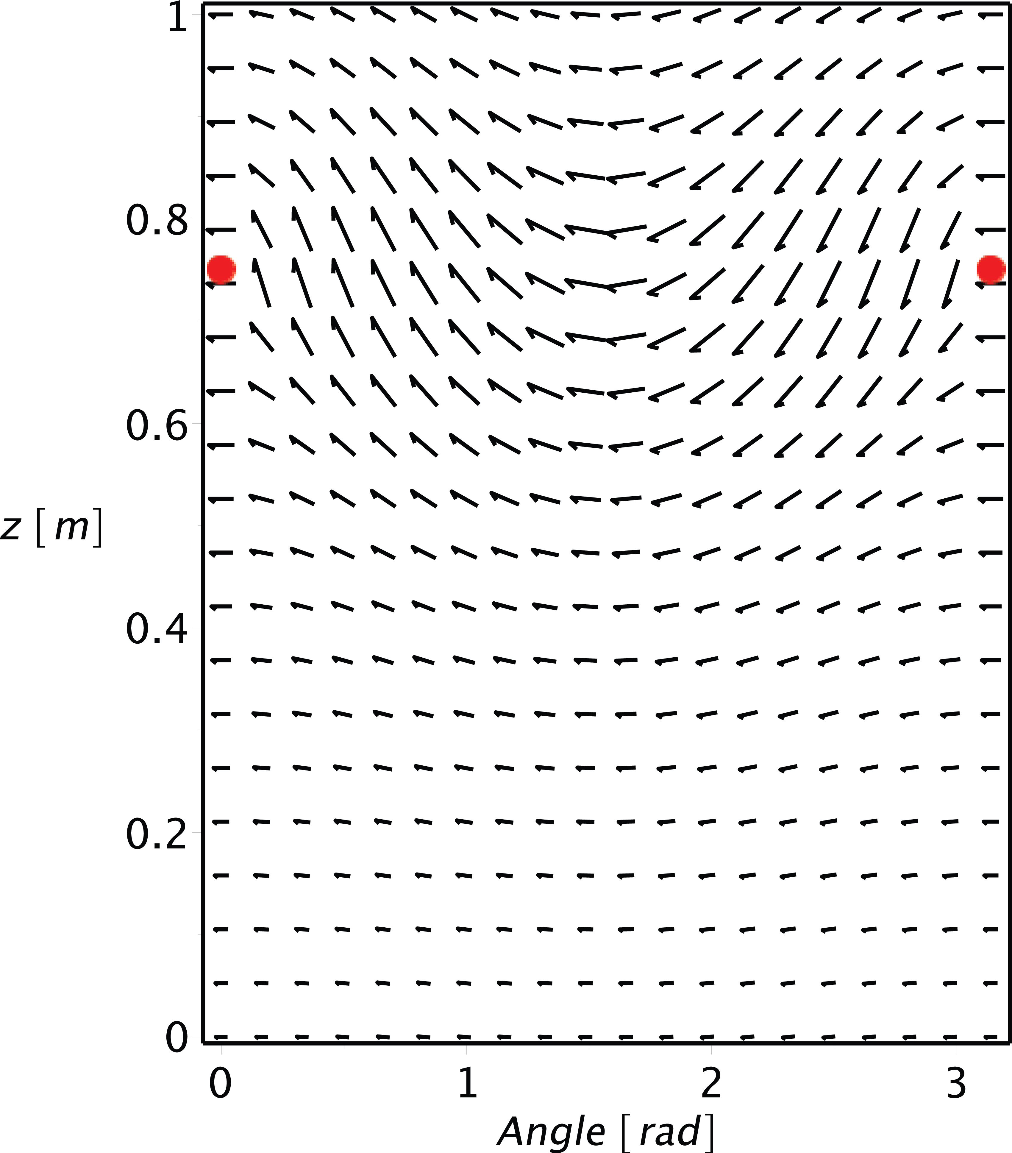
Representation of the gradient of Δt values for a pair of two sensors (dots) along the outer surface of a pressure vessel.
For improved visibility, only half of the vessel surface is depicted in Figure 2. Here, only the gradient of Δt values for the two sensors marked in red is shown. For these, it may be observed that the change in the Δt values is maximal directly between the two sensors, and it decreases with distance from the sensors. The maximum gradient of Δt values expected in the investigated pressure vessel is approximately 277 µs/m and the minimum is 226 µs/m. These values directly result from equation (3) using the known source and sensor positions and assuming a quasi-isotropic sound velocity, which was chosen as average sound velocity measured in our pressure vessel. It can also be seen that the change with spatial distance is lower in the immediate vicinity of the sensors.
These estimates represent a rough approximation of the real conditions in the CFRP/steel pressure vessel and are meant to serve as an estimate for the determination of the uncertainty of source localization. It should be noted that the material for these assessments is assumed to be isotropic and thus only represents a first approximation, but was found to be in good accordance with the results from our experimental measurements.
Limitation of source localization accuracy based on Δt values
In order to derive the source localization accuracy in our experimental setup, this section provides an overview on relevant sources of uncertainty. Typically, distinction is made between statistical variations and systematical variations of a value. In the following two subsections, the impact of several experimental parameters on the quantities entering equations (1) and (2) is discussed. In the third subsection, the resultant lower limit of source localization accuracy is derived. To facilitate the reading, all parameters are discussed in application to the experimental setup described in section “Experimental setup” and as shown in Figure 1.
Parameters with statistical variation
As first step, only parameters with statistical variation are discussed. All following derivations use the conventional definition
Uncertainty of the grid position
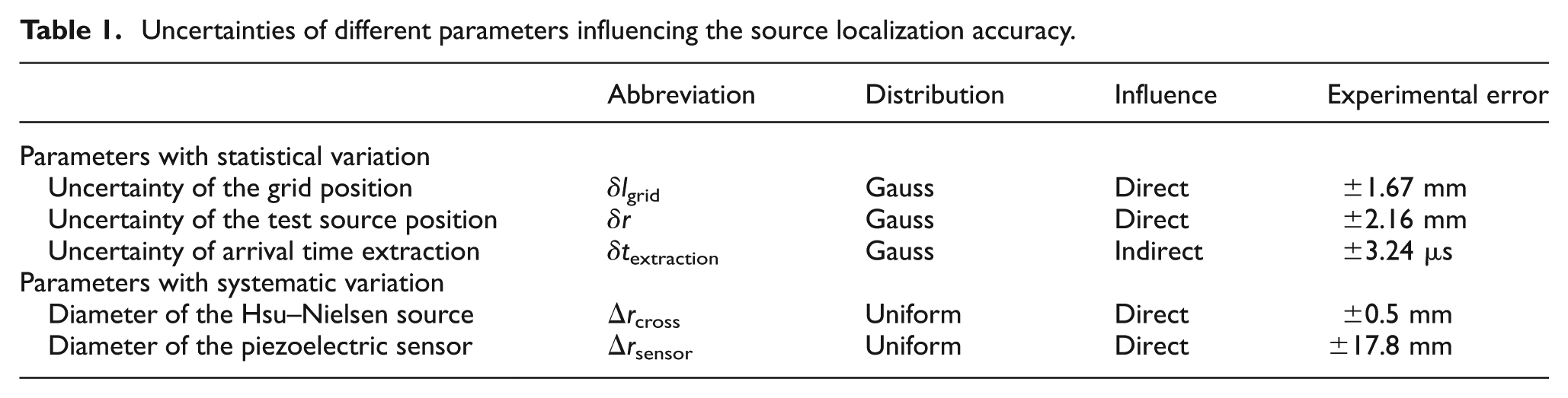
This uncertainty is based on the finite thickness of the grid lines and the accuracy of drawing the grid. The grid lines were applied using a white marker with a variable thickness of approximately 0.4–3 mm depending on the applied pressure. The deviation of the grid position relative to the nominal value was quantified at 10 different points on the pressure vessel, which resulted in a total uncertainty of ±1.67 mm with Gaussian distribution. This uncertainty has a direct influence on the localization results since it affects the position of the source coordinate
Uncertainty of the test source position
This uncertainty is caused by the possible deviation of the test source position relative to the source coordinate
Uncertainty of arrival time extraction
One major uncertainty is given by the extraction of the arrival times from the waves. Since the initial part of the wave is a rising slope, the exact definition of a signal arrival is generally difficult. The methods using constant threshold values to detect the signal arrival depend substantially on the slope of the initial part of the wave and, therefore, may cause scatter of the so obtained Δt values. But even versatile approaches for picking the time of arrival like the Akaike information criterion (AIC)
21
are sometimes error-prone. Specifically for the AIC function, the absolute minimum is sometimes way apart from the real signal arrival. This happens for instance, when multiple guided wave modes arrive at distinct times with later arriving modes being stronger than the first mode. For a set of signals, the deviation of arrival times to the real value may be assumed to be randomly distributed. To quantify the uncertainty for this parameter, 10 randomly selected waves were examined and the mean deviation between manual and automated signal arrivals was quantified. The so obtained uncertainty was ±3.24 µs and is assumed to be Gaussian distributed with direct influence on the arrival times
Parameters with systematic variation
Systematic influences can affect a measurement by a constant offset or by linear or even non-linear scaling. Therefore, the measurement result should ideally be compensated with respect to all known systematic variations, which is hard to achieve in practice.
Influence of test source dimension
Since the test sources used in the experiments have a finite dimension, their influence is discussed first. The piezoelectric pulser used in the experiments has a diameter of 17.8 ± 0.5 mm, and the Hsu–Nielsen source has a diameter of 0.5 ± 0.01 mm. Scatter of both values was found to be specific for the respective piezoelectric pulser and the respective pencil lead. The distribution of this parameter is assumed to be uniform and the uncertainty of this parameter on the test source position
Influence of sensor dimension
There is an aperture effect which is caused by the piezoelectric sensors which have a diameter of 17.8 ± 0.5 mm. The detection of the wave is therefore distributed over a certain area. The assumed source–sensor distance may thus range from X + 8.9 mm to X − 8.9 mm depending on the angle of incidence.
Uncertainty caused by dispersion and attenuation
There are various dispersion effects which can affect the arrival time measurement more or less significantly. The effects of dispersion can be subdivided into chromatic and modal dispersion. Chromatic dispersion is dependent on the wavelength and the type of wave (i.e. longitudinal or transversal). The impact on the detected wave depends on the specific materials and in composites also on the propagation direction. 22
Since a fracture process is not monochromatic, the wave propagates with lower velocity at lower frequencies. 22 This leads to the effect that higher frequencies of an acoustic wave are detected first and therefore determine the time of arrival.
However, in thin-walled structures such as the pressure vessel studied herein, modal dispersion occurs as well. Modal dispersion arises for guided waves, such as Lamb waves typically found in plates, which can be described by the Rayleigh–Lamb equation. 23 The modal dispersion effect overrules the chromatic dispersion in such structures by some orders of magnitude. In the case of Lamb waves, the acoustic wave propagates as characteristic symmetric and asymmetric modes which will be referred to as Sx and Ax, respectively. The index x is an integer which starts with 0 for the fundamental mode and 1, 2, 3, … for higher-order modes. If the fundamental symmetric mode S0 is excited by the acoustic emission source, it will define the time of arrival since this is the fastest wave mode at reasonably low frequencies. If this is not excited, other modes will determine the first signal arrival. This plays a significant role in classical source localization since the propagation velocity of the modes can change substantially resulting in a respective error in the source position calculation.
This only exemplifies the high complexity of a dispersion-based influence on the accuracy of localization algorithms. Also, this influence is not always feasible to consider explicitly, since it is strongly dependent on the sensor position, the propagation path, and the source type.
Another significant effect to consider for the localization accuracy is the attenuation. This takes place in the form of geometric spreading of a wave from a point source which propagates circular in all directions. Additionally, dispersive losses due to scattering or frequency-dependent absorption may take place. As demonstrated by Hosten, 22 the frequency-dependent attenuation is different for longitudinal or transversal waves and the attenuation coefficient increases with frequency. This may result in a detection of the high-frequency components of the S0 mode for nearby sensors, whereas distant sensors may only detect the low-frequency components of the A0 mode.
Uncertainty caused by other effects
The factors discussed above are generally known and may have the highest impact on the localization accuracy. However, there are plenty of other factors that can also affect the localization accuracy more or less significantly. Factors like the sampling rate influence the temporal measurement directly with a standard deviation of ±28.87 ns, which can be neglected in comparison with the other parameters. Also, the uncertainty caused by the sensitivity variation of the sensor can be important. Each acoustic emission sensors is known to have a unique sensitivity within a given frequency range. Due to resonances it is possible that the sensitivity is magnitudes higher for a specific narrow frequency range than for other non resonant frequencies. It is possible that signals which are within a resonance of an acoustic sensor are predominantly detected, whereas others which may have the same or even higher amplitudes are detected with a lower amplitude or not at all. This leads to a systematic influence of the sensor to the measurement and the results.
It is also possible that inhomogeneities in the material are present which interfere with the wave. This is, for example, the case if holes or fixtures are attached to the structure. Also, voids or other defects in composite materials may cause a disturbance of the wave field. Such an inhomogeneity or discontinuity can even distort the wave propagation in a way that no direct path from the source to the acoustic sensor exists. Therefore, the signal arrival time is based on indirect reflections and causes respective measurement errors.
Furthermore, there are also purely thermal effects which will not only cause thermal expansion of the involved geometries but may also contribute significantly to the noise level, as well as to the properties of materials and thus the transmission characteristics.
These are just a couple of examples to mention in the context of this work. A detailed discussion of all effects is not part of this publication and also not subject to the assessment of uncertainty in this case. Instead, Table 1 summarizes the discussed parameters with a significant relevance to the localization problem in the presented setup including their influences on the measurement parameters determining the source localization accuracy.
Uncertainties of different parameters influencing the source localization accuracy.
Absolute limit of source localization accuracy based on Δt values
For a technical classification of a localization algorithm and its accuracy, it is possible to perform a relative comparison with existing methods. However, knowing the absolute limit of source localization accuracy in a specific setup allows determining whether the method may still be improved or has already converged to its technical limits.
To derive the lower limit of source localization accuracy, only the parameters with statistical variation will be taken into account. This is due to the challenge to account for the effects of systematic variations in parameters as found in Table 1. Nevertheless, neglecting these uncertainties will simply lead to a more optimistic lower limit, that is, in reality the source localization accuracy will even be less.
In the first approximation, the parameters discussed in Table 1 are uncorrelated, which allows the use of the simplified version of Gauss’ formula for a specific parameter
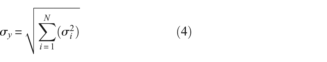
Here,
The uncertainties of
Applying equation (4) and the values of Table 1, the resultant source localization error of
Here, it is worth noting that the presented neural network approach directly incorporates systematic parameter variations, since these are implicitly modeled in the training stage (cf. section “Neural-network-based source localization”).
Neural-network-based source localization
The basic idea behind neural networks is that through the connection of simple individual elements, a network is created that can capture or process complex information. As research in the field of ANN has its origins in neuroscience, the terminology of neuroscientists is generally used to describe elements and processes in ANN. For example, the basic nodal elements of the networks are called artificial neurons. These neurons are coupled via weighted connections to form a network.
The advantage of these networks is their capability to recognize patterns and symbolic contexts from examples without using explicit analytical functions to describe this context. This is usually achieved through a modeling phase, where an ANN structure is trained based on a representative dataset. Hence, this process is generally called the “learning” or “training” of the network. During this phase, a symbolic functional relation between the input data and output data is approximated that reproduces the characteristics inherent to the system. Subsequent to the modeling phase, the ANN can be used for predicting the output data values based on arbitrary input data values.
In general, there are unsupervised and supervised learning methods, which differ in that unsupervised algorithms cluster the measured values according to their internal structure, 24 whereas supervised methods try to model a symbolic functional relationship that is inherent in the system. The function approximation required in the case of acoustic emission source localization requires a direct relation between an input dataset to a corresponding set of output data. Therefore, only supervised learning methods are suitable for this purpose. The network used in our case is called the feed-forward network because no internal feedback loops are present. The network output is compared with the target pattern and fed back only at the end of one iteration cycle.
Distinction is made between the input layer, the output layer, and the layer of “hidden” neurons, also called the hidden layer. The number of neurons in the hidden layer significantly determines the maximum complexity of the network.
Any neuron in the network obeys the following formula
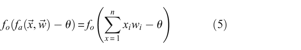
where
An ANN with purely linear activation functions is only able to approximate linear problems because coupling of any number of linear elements still only yields a linear function. Such linear neurons are hence used to correct linear offsets that may occur in a data structure.
In principle, whether a sigmoidal (hyperbolic tangent) or radial (Gaussian) basis function is chosen is irrelevant if suitable training and a sufficient number of neurons are provided. However, the choice of the basis function should match the expected value distribution of the used data. A radial basis function better fits problems that are of radial symmetry in their structure, whereby non-radial problems can also be modeled by just scaling the flanks of a radial function. The symmetric part of the radial basis functions is then scaled so that it resides in the untrained or non-relevant regions outside the investigated data structure. Because no symmetrical data structure is expected for a general source localization problem, a hyperbolic activation function is used instead. This has also been experimentally found to be the most suitable activation function.
For the acoustic emission source localization, networks with a fixed number of neurons are used. Adjustment parameters are the threshold value of individual neurons, as well as the gain and inhibiting connections. It is also possible to delete or re-establish connections.
During the modeling phase, the network weights are changed according to the input and output parameters of the dataset. A critical issue during this modeling phase is the “training algorithm” of the network which is used to achieve a sufficient approximation. To this end, the current network output is compared with the desired output and the network weights are then optimized accordingly via a feedback loop. The training method that is most suitable for this type of function approximation problem is called backpropagation and is a standard procedure, which is described in detail by Bishop. 25
The input dataset or training dataset is usually subdivided into fit points and validation points. Using the fit points, the network weights are adjusted. The validation points are not used for the weight adjustment, but for the decision whether the trained neural network is able to predict unknown (the validation) points. These two datasets serve the functions of modeling and evaluating the neural network during the training phase. In further derivatives of neural networks, there is another set of unknown test points that are used to rate the final quality of the present training state of the completed neural network.
The quality of the neural network can be evaluated using fit and validation points. Typically, if the number of neurons and layers is gradually increased, the fit quality improves accordingly. Such improvement can be evaluated on the basis of the R2 (root-mean-square error (RMSE)) and the average deviation of the predicted output data to the known output data. The optimal number of neurons and layers is reached when the model quality does not change significantly by adding additional neurons or layers.
The training procedure, the resulting neural networks, and their approximation quality are influenced directly by the chosen error function. Usually, a quadratic error function is used, which calculates the deviations between the network output generated from a given input and the target value (known output value). The resulting deviations are then squared and summed over all points using formula (6)
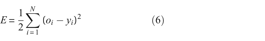
The variable E is the resulting error over all patterns, N is the number of training data points, y is the predicted output value for a known input x, and o is the known output value.
The minimum of this error corresponds to the optimum model. The choice of a quadratic error function, however, is only advisable if the model is not dominated by outliers or if the number of training points is high. If the training point density is low, a single strong outlier (e.g. a measurement error) can significantly distort the network because the network does not decide whether training points are relevant or just measurement errors. At a high number of training data points, however, the weight of a single outlier is less strong. Therefore, it is very important to use the best possible input data for the training phase, especially if the overall number of training points is low. From the viewpoint of neural network optimization, the “best” data basis exhibits least scatter and correlates as high as possible to the source location coordinates.
The required number of training points is dependent on the number of neurons and the complexity of the system. For the fit of a neuron in the network, the offset of each neuron and the input weights must be adjusted. This means one needs a number of weights at least as large as the degrees of freedom leading into the neurons and an additional offset. In practice, it has been proven that at least twice as many training points are required as the number of weights present in the network.
However, there are no strictly defined limits for the number of training points. As a rule, higher number of training points results in a more accurate neural network approximation, and vice versa. If a target accuracy is required, additional training data points can be iteratively added to the model to increase the neural network quality.
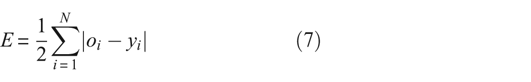
If the training data points face some outliers despite a previous cleaning of data points using plausibility (e.g. by specifying a maximum Δt value), the choice of error function needs to be adjusted. In this case, the use of the sum of the absolute values is recommended. This does not emphasize strong outliers and offers the advantage of a strong weighting and an equally distributed error weighting of all training points
It is also useful to apply an additional penalty method that is added to the error function to limit the magnitude of change in the weights during each iteration of the training phase. These limits usually lead to better generalization and yield a more smooth functional approximation. More detailed information on these implications can be found in the standard literatures such as in the studies by Bishop 25 or Haykin. 26
A large error during the training phase indicates too few degrees of freedom or too few neurons in the network. On the opposite side, a small error during the training phase in comparison with the validation error may indicate that the network does not adequately generalize the data structure. The latter would imply that the network has too many degrees of freedom, and the number of neurons should be reduced. Following such guidelines, the probability of overfitting is reduced. This effect may occur when too many neurons are used in the network. If neural networks are trained repetitively using the same dataset, it is possible to evaluate the overall network quality by the distribution of the individually achieved network qualities and their resulting deviations from the input data.
Experimental setup
In this section, the experimental setup used in this study is described. For the detection of acoustic emission signals, seven multiresonant sensors (type WD; Mistras) were mounted on a type III CFRP pressure vessel with metallic liner using suction cup holders. To provide a suitable acoustic transmission, a medium viscosity silicone paste (Baysilone) was used as a couplant. All signals were detected using a PCI-2 acquisition system with 40 dB preamplification, 45 dB threshold level, and 20 MSPS sampling rate. A sixth-order Butterworth bandpass was chosen to range from 1 kHz to 3 MHz. The data acquisition software AEWin is used, whereas further analysis is done with the software language R using the statistical package “constrOptim,” the “neuralnet” package, and the software environment SPSS.
Acoustic emission signals were introduced using two different test source types to ensure the excitation of different frequency ranges. As one type, the classical Hsu–Nielsen source was used, 27 and as second type, a piezoelectric pulser was used to also excite dominant frequency parts above 100 kHz (cf. Figure 4). For the latter, the applied rectangular pulse had a rise time of 2 ns and a duration of 20 µs, followed by a falling edge of 2 ns and a maximum amplitude of 10 V. These settings were experimentally found to be the best compromise between signal amplitude and frequency bandwidth of the resulting acoustic emission signal. These two test source types are intended to simulate the broad bandwidth of acoustic signals that may occur in real CFRP structures. For the determination of the signal arrival, AIC is used. 6
The pressure vessel is 1.08 m long and has a diameter of 33.3 cm. The lateral surface has a length of 79 cm, and the dome has a radius to the top of 14.5 cm. Five of the seven sensors are located on the cylindrical surface and two more sensors sit on the dome of the vessel, as shown in Figure 1. The cylindrical part of the vessel has 12 × 18 grid lines, which are further branched on the spherical dome to yield additional 19 partitions. At all 444 junction points of the grid, an acoustic signal is excited by each of the test source types. Furthermore, two cases are distinguished in the following. As first configuration, the source localization is carried out using an empty vessel, and then, as second configuration, using the vessel filled with water. This means the total database of signals was 12,432 acoustic emission signals generated and measured, which will be used for the source localization procedure in four test cases.
To maintain consistency of the approach and to ensure comparability between the classical localization method and the method using ANN, for both localization procedures, the same Δt values are used as input database. All Δt values of seven sensors are used, whereas the vessel surface is projected to a 2D grid. That means there are 21 sensor pairings.
Due to the arrangement of the acoustic emission sensors on the vessel surface, it can be depicted that it is not useful to use all pair-wise combination of seven sensors for source localization since it is expected that signals occurring close to the vessel bottom exhibit the longest propagation distance to the sensors on the vessel dome and thus suffer most from attenuation and dispersion, which causes a high error of the determined Δt values. For this reason, only five sensor pairs are used simultaneously which means the calculated source position is overdetermined twice. The most likely source position is then determined from the scatter of source positions of all subset combinations from five out of seven sensor pairings. The subset combination with least scatter respectively the lowest error is chosen for the determination of the final source position. The possible values for the x value are limited by the physical size of the tank ranging from −10 to 80 cm, whereas zero is an arbitrarily defined symmetry axis. The y direction is limited from −20 to 150 cm accordingly. The sound velocities used for the localization procedure are 5636 m/s in the x direction and 4230 m/s in the y direction. Both velocities were obtained from previous measurements of arrival time differences evaluated along the axial and circumferential axis of the pressure vessel. To this end, two WD (Wideband Differential) sensors with 200 mm distance spacing and 15 test source positions were used as data basis.
Using the techniques described in section “Neural-network-based source localization,” a two-layer network with 4 × 4 neurons with a hyperbolic tangent activation function was chosen. This number of neurons was found to be optimal by gradually increasing the number of neurons and iteratively checking the according fit quality parameters described in section “Neural-network-based source localization.” The optimal number of neurons and layers is reached when the model quality does not change significantly by adding additional neurons or layers. The initial learning rate is chosen as 0.001 which can be varied by the network during training with a change rate coupled to the error function.
Up to 5000–10,000 models are fitted to one training dataset and the best one is selected based on the model parameters. If all 444 waves of the dataset would be used for the neural network training and validation, one could reach arbitrarily accurate source coordinates. To avoid such overfitting of the source coordinates, we use only one quarter from the dataset (i.e. 111 waves) as statistically representative subset for training and validation. The training dataset is further subdivided into 74 fit points for the training and 37 validation points. As input data structure, all 21 Δt values are used with an output vector of x and y coordinates. For the selected 111 test data points on the vessel surface, the resulting model quality is consistently repeatable with respect to the variance of the model parameters. A further increase in the training data density leads to models with lower variance, but a substantial decrease in this variance was found to be inhibited by the scatter of the measurements. Aside from the 111 test data points, the remaining three quarters of data points are unknown test point positions, which are further used to determine the localization accuracy.
Results
Acoustic emission wave propagation
In order to understand the impact on source localization accuracy, some common aspects of wave excitation and propagation in the type III pressure vessel are discussed first.
As pointed out in section “Experimental setup,” two different acoustic emission test sources were used to yield different parts of the frequency spectra. In general, the types of signals encountered in hybrid CFRP/metal structures can cover a broad bandwidth and may excite multiple modes. 28 Hence, it is important to replicate the acoustic emission signals of different failure mechanisms in their key characteristics when being used as input data for Δt-value-based source localization.
To compare the differences in bandwidth, the Choi–Williams distribution of one signal of each test source is shown in Figure 3. The top figure shows the time–frequency profile of a signal due to a Hsu–Nielsen source placed in 523 mm distance to the sensor. The source position is on the surface directly opposite the sensor position, so the signal traveled 180° around the vessel to the sensor position. For the Hsu–Nielsen source, the signal is found to be predominantly a low-frequency signal width, a bandwidth up to 100 kHz. The high-frequency parts are less intense, but still present as seen by the faster mode in the beginning of the signal between 150 and 280 µs. These weak modes likely fall below the detection limit (e.g. noise level) after a certain distance of propagation and therefore may yield unstable evaluation of the signal arrival times.
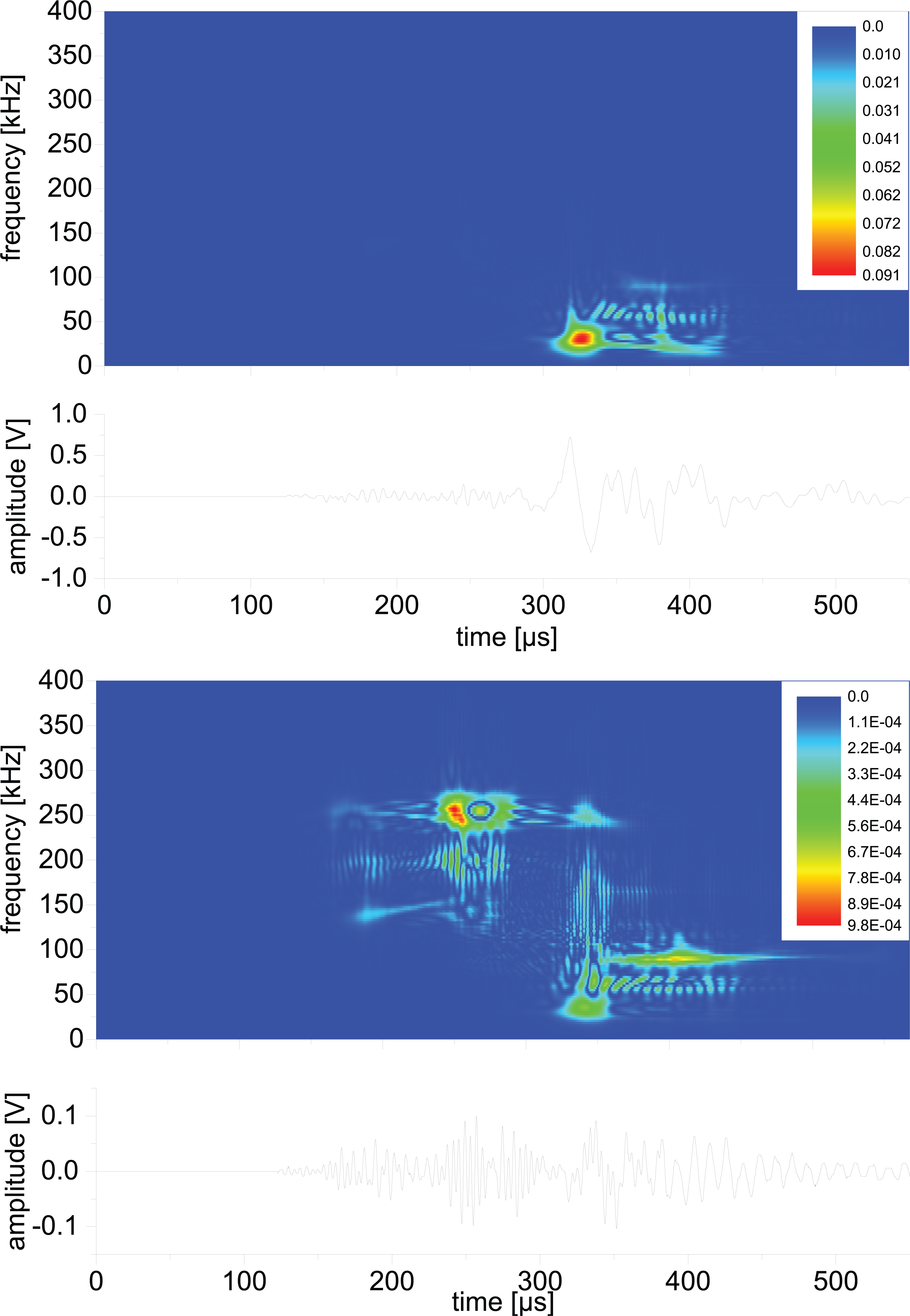
Frequency–time profile of an acoustic emission signal detected in 523 mm distance to the sensor (top: Hsu–Nielsen source; bottom: piezoelectric pulser).
The bottom image of Figure 3 shows the signal due to excitation from a piezoelectric pulser after detection in 523 mm distance. It can be observed that a frequency range up to 300 kHz is excited. In particular, the mode in the beginning of the signal is more intense than for the Hsu–Nielsen source. Therefore, this test source type offers a different bandwidth, which can be used to represent other signal types as seen in testing of composite materials.
Another effect relevant to the investigation of pressure vessels, which is described in the literature, is the possibility of a water path propagation. 8 This possibility arises due to two propagation paths if source and sensor are approximately on the opposite sides of the vessel. Here, the acoustic propagation path as guided wave on the wall of the pressure vessel and the direct propagation path through the contained liquid are coexistent. Although the direct propagation path in the contained liquid is shorter, the sound velocity in liquids is typically much slower than in the fiber-reinforced wall. Hence, the origin of the first signal arrival is not always straightforward to attribute to the guided wave or the direct signal arrival, respectively. Also, the guided wave propagation in a liquid–solid–gas configuration will not only cause simple plate wave propagation but also is likely to excite leaky Lamb waves. 29 Other effects such as the initial (gravity) loading of the vessel by the contained liquid may result in further changes of the signal propagation due to compressive forces acting in the supports or by closure of air gaps in between the pressure vessel and the support structure.
In Figure 4, acoustic emission signals are shown that are detected directly opposite to the acoustic emission source position in 523 mm distance. Comparison is made between the acoustic wave in the empty vessel and the acoustic wave in the vessel filled with water for each of the two test sources. As seen by the changes in the signals in Figure 4, the presence of the water fill has an impact on the signal propagation. For the Hsu–Nielsen source signals, it is possible that the apparently earlier arrival of the lower frequency part (indicated by an arrow) is actually the water path, as discussed by Hamstad. 8 It is also possible that the occurrence of leaky Lamb wave propagation in the filled vessel causes further changes and hence changes in the signal characteristics. There is also a change in the acoustic emission signal of the pulser as seen in Figure 4. The shares of the higher frequency mode are attenuated more than the lower frequency shares. However, a direct indication of the water path arrival is not observed here.
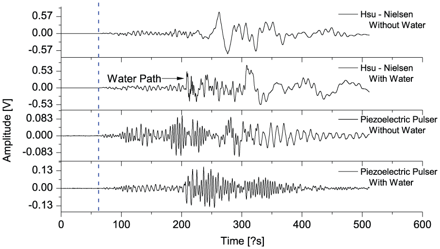
Acoustic emission signals from different test sources in water-filled and empty pressure vessel detected at 523 mm distance.
In both cases, the observed effects will have an impact on the extracted signal arrival times and, therefore, influence the localization accuracy of a method that does not take into account such changes. In particular, the occurrence of a water path signal arrival and the frequency-dependent attenuation 30 may cause step-like changes in the extracted signal arrival times and will therefore affect the localization accuracy. Hence, the chosen configurations are used to examine the impact of those effects on the localization accuracy in the tested localization methods.
Classical source localization method
To start with the comparison of the localization methods, the results of the classical source localization method as described previously are presented. All four cases investigated are shown in Figure 5 as false color map of the source localization results. To this end, the spatial deviation between the (known) position of the test source and the calculated source position is represented by the color range in the image. This deviation will further be referred to as source localization error. Interpolation between the measurement points is carried out using a thin plate spline 31 with a constant smoothing parameter of 0.01. Hence, positions with strong deviations to the real source position are of red color and signals, which could not be localized, are given a gray color. For all cases, the respective source localization error is in the range from 0 to 25 cm, whereas the gray areas indicate regions, where the test source signals could not be localized. The light gray area represents a deviation that is greater than 25 cm.

Localization results on one half of the pressure vessel using different test source types for a filled and for an empty vessel using the classical localization method. The color coding represents the source localization error in centimeters.
It can be observed that there is a systematically stronger deviation close to the sensor positions. This is because the gradient of Δt values is lowest close to the sensor positions, and therefore, the same error in Δt values leads to a larger error in source location. It is also evident that the dome has a lower localization accuracy for all four configurations. This is mainly due to the curvature of the dome, the possibility of multiple reflections, and interactions with the pressure inlet (located at the tip of the dome). Furthermore, the sensors are on the dome and are particularly close in position, which means that sensors 3 and 4 face the same problem of low Δt-value gradients in the near field. All of these effects add to the lack of quality of the localization.
The localized Hsu–Nielsen source positions have an average deviation of 7.0 ± 10.2 cm for 419 out of 444 points. The standard deviation is greater than the mean value, which indicates the significant scatter of the calculated results. The localization quality decreases substantially for the test signals excited by the piezoelectric pulser. On the dome, almost no points were localized and only 199 of the 444 points were localized at all. The calculated source positions show a mean deviation of 14.0 ± 16.1 cm to the real position. For comparison, the results of the water-filled vessel are also shown in Figure 5. The number of localized test source positions decreases further for both test source types. For the Hsu–Nielsen source, the amount goes down from 419 to 407, with a mean localization error of 6.9 ± 6.2 cm. For the piezoelectric pulser, only 167 points could be localized, with a mean localization error of 14.9 ± 12.9 cm.
Neural-network-based source localization method
For the same input data, the source localization results are now presented for the neural network structure discussed in section “Experimental setup.” The representation of the results shown in Figure 6 uses the same configurations as discussed for the classical source localization procedure. In particular, the false color range is chosen to be identical to Figure 5. On the left side of Figure 6, the source localization error of the piezoelectric pulser and Hsu–Nielsen source for an empty vessel is shown. On the right side of Figure 6, the respective images of the water-filled vessel are shown. For all cases, the respective source localization error is in the range from 0 to 25 cm, whereas the gray areas indicate regions, where the test source signals could not be localized.
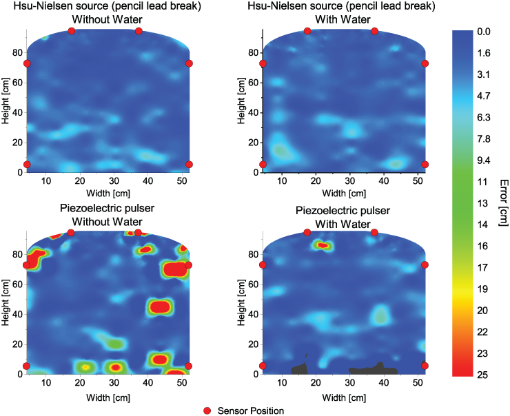
Localization results on one half of the pressure vessel using different test source types for a filled and for an empty vessel using the neural-network-based localization method. The color coding represents the source localization error in centimeters.
In all configurations, the change in source localization error close to the sensor positions is difficult to spot. This is because the changes of the Δt-value gradients can be compensated by the neural network in the training phase. It can also be observed that for the same reason, the source localization error is almost identical in all parts of the vessel. Especially at the dome, this leads to a substantially good source localization quality.
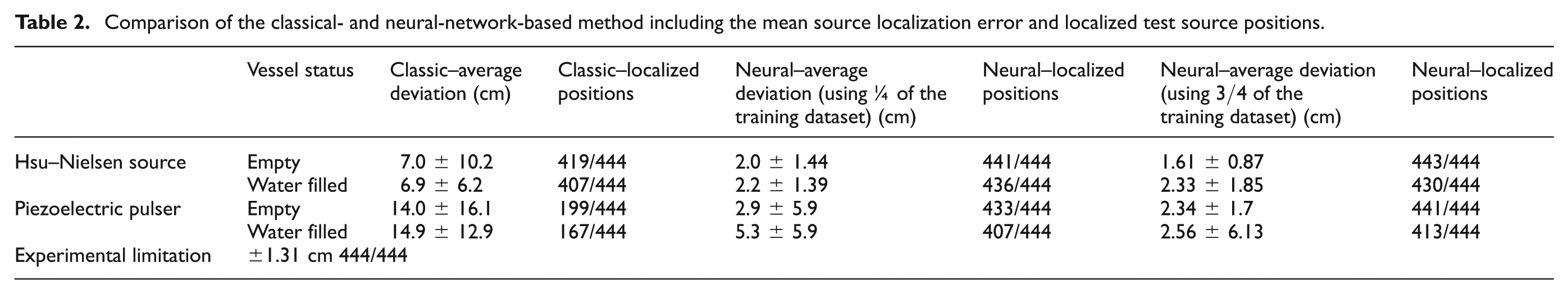
In terms of statistics, the Hsu–Nielsen source in the empty pressure vessel has a mean source localization error of 2.0 ± 1.44 cm for 441 out of 444 test points localized. This accuracy can be achieved using one quarter of the data points as training and validation points. The mean error (RMSE) during the training and validation is 2.21 cm. This shows that the approximated error during training and validation can be used for predicting the source localization error of unknown points, assuming an adequately trained model. Also, the quality of a model can be improved using additional data points for the model building. The improvement reaches an upper limit with 333 training and validation data points which equals three quarters of the measured points. The resulting source localization quality equals 1.61 ± 0.87 cm for 443 out of the 444 test points localized. The increasing accuracy can also be seen in the RMSE of the model. Therefore, in the following, only the accuracies of the best-fit models will be discussed in detail. The results of all training datasets can be found in Table 2.
Comparison of the classical- and neural-network-based method including the mean source localization error and localized test source positions.
For the broad bandwidth excited by the piezoelectric pulser, the localization quality in the empty pressure vessel is slightly lower having a mean localization error of 2.34 ± 1.7 cm, based on 441 out of 444 points localized. In the water-filled vessel shown on the right side of Figure 6, the source localization error increases slightly. The number of localized test source positions decreases for the Hsu–Nielsen source from 443 to 430, with an increasing localization error of 2.33 ± 1.85 cm. For the piezoelectric pulser, 413 source positions were localized having a mean localization error of 2.56 ± 6.13 cm.
Comparison between classical- and neural-network-based source localization
It is evident that especially in the classical source localization, the deviations to the test source position are of systematic nature. The localization quality close to the sensor positions is slightly worse in both approaches, but these characteristics are less pronounced in the neural-network-based approach. The localization error in the center of the rectangular plane defined by the sensor positions is generally lower than elsewhere on the vessel surface. Since the origin of this effect is the gradient of Δt values, this can also be observed in the neural localization, although considerably less distinct. Another detail that differs greatly between the two methods is the localization accuracy as well as the general possibility to localize sources at the dome region of the vessel.
For the broader bandwidth offered by the signals of the piezoelectric pulser, the localization error was generally found to be different for the Hsu–Nielsen source. This systematic variation in the localization accuracy may be caused by different attenuation levels for the higher frequencies. Even using the AIC method, this may lead to selection of the arrival time of different wave modes, especially if the fastest mode drops into the noise level after a long propagation path to the sensors. This may generate a systematically different Δt value than after signal detection after a short propagation distance. This effect cannot be compensated by the traditional localization method, which therefore results in a systematic error. In the neural-network-based approach, though, these effects can explicitly be accounted for in the training phase.
Table 2 holds the comparison of the source localization errors of the classical source localization method and the neural network method for all four configurations. It can be observed that the classical source localization method has a worse accuracy than the neural-network-based method in all investigated cases. In summary, the accuracy of ANN was found to be superior by a factor of 3 to 6. The scatter of the localized source positions is also positively affected by the use of the neural-network-based approach, which causes a reduction in a factor of 2 to 11. Also, the total number of localized test sources is substantially improved.
Considering the theoretical error calculated in section “Theory,” the neural-network-based source localization with a mean error of 1.61 ± 0.87 cm is within the range of scatter of the expected experimental limits of approximately 1.31 cm. Consequently, the determination of the arrival time of the measured data must thus be improved to achieve any further significant reduction in the source localization error based on Δt values.
Conclusion
It has been demonstrated that an acoustic emission source localization method using neural networks is superior to the currently established classical method in all cases investigated. The comparison is based on identical input data provided by experimentally obtained Δt values, thereby allowing a quantitative comparison of the two approaches.
The average source localization accuracy is better by up to a factor of 6, and the variation around that average is lower by as much as a factor of 11. The neural-network-based approach was also possible to improve the number of localized acoustic emission events by a factor of 2. Additional factors of influence such as the excitation of a different bandwidth, as well as indirect propagation paths including reflections and a geometrically complex and curved propagation medium, did not lead to significant reduction in the source localization accuracy of the neural-network-based method.
It could further be shown that for the Δt values as input data, the accuracy of the neural-network-based source localization accuracy approaches the limits of the theoretically expected source localization accuracy. Therefore, any further increase in the source localization accuracy can only be achieved by substantial improvement in the input data used for the training stage of the neural network. This could either be done by alternative strategies for determination of the signal arrival or using alternative values extracted from the detected acoustic emission signals.
Footnotes
Declaration of Conflicting Interests
The author(s) declared no potential conflicts of interest with respect to the research, authorship, and/or publication of this article.
Funding
The author(s) disclosed receipt of the following financial support for the research, authorship, and/or publication of this article: This study was funded by the German Federal Ministry of Education and Research (03MAI12A) within the project MAI zfp within the leading edge cluster MAI Carbon.