
Abstract
Scour is the main cause of bridge failures. Monitoring of bridge scour is an essential method to control the damages caused by flood events. In this study, a large-scale tube consisting of heating and temperature-sensing elements was developed, and its application for detecting saturated soil and water was analyzed. Laboratory experiments confirmed the applicability of the thermal sensor for scour-monitoring purposes. Three methods are proposed in this article for analyzing the data obtained from a heat probe. A linear relationship between temperature increase from the initial to the secondary time and heat production in the probe was observed, and a line that can be used to determine scour was introduced. This method is simple and can be used for low-cost, large-diameter heat probes that are easy to fabricate.
Introduction
Washing away sediments around bridge piers and abutments leads their foundations becoming unsupported, and they may collapse suddenly. This phenomenon is called scour, and it is the main cause of bridge failures. The approximate estimations based on theoretical and experimental relationships are not adequate for predicting the exact behavior of scour holes and bridge abutments or piers.1–5 According to the Federal Highway Administration (FHWA) guidelines, scour-critical bridges should be monitored and/or have scour countermeasures installed. 6 Different scour countermeasure methods are used to prevent failure of bridges that are subjected to scour and the associated loss of life.7–9 Monitoring is usually the least expensive of these methods. Sonar, magnetic sliding collars, float-out devices, tilt sensors, time-domain reflectometers (TDRs), and sounding rods have been recommended for use as fixed scour-monitoring instruments.10–15 The main ideas of these methods are that water and soil (especially saturated sand, such as riverbed material) have different properties and that sensor can detect whether they are located in water or sand by measuring these properties.
The thermal properties of water and soil are different, so thermal sensors can be used for scour monitoring. One method could be to measure the temperature of the places where sensors have been located, but this is not an acceptable approach, 16 because temperature varies throughout the day and night and also variance of temperature in different seasons of year influences it. Also, temperature varies with depth. So, because of these effects, the temperature measurement would not be an effective and reliable method for scour monitoring.
Heating the medium and monitoring the changes in temperature during heating and cooling periods have been used to study the nature and structure of materials. Thermal sensors have been used for measuring the thermal conductivity of materials and the water content of soils. 17 Heat probes have been used for many measurements, that is, heat flux in the Atlantic Ocean, moon explorations by Apollo 15 and Apollo 17, and Mars’ thermal properties by NASA’s Phoenix mission. 18 Heat dissipation is different in water and soil, and this can be used to distinguish these media from each other. This method is known as active thermometry. 19
Heat can be transferred by conduction in materials. For example, heat transfer in saturated soil is based on conduction. Thermal conductivities have been measured for saturated Ottawa sand C-109, Ottawa sand C-190, and Toyoura sand, and they have been reported to be between 2.35 and 3.31 W/m K. 20 Heating a probe in water causes natural convection, which means that heating leads to changes in density. Convection is heat transfer that occurs due to fluid motion, and it increases the rate of heat transfer through the fluid. Convective heat transfer is a complicated phenomenon, and it depends on many parameters, such as dynamic viscosity, µ, thermal conductivity, k, density, ρ, specific heat, Cp, and velocity, V, of the fluid, and the type of flow, for example, laminar or turbulent flow. Heat transfer also depends on the properties of the solid that is in contact with the surrounding medium, such as its geometry and the roughness of its surface. 21
In the research reported in this article, a large-diameter heat probe was built and used to monitor scour. This article is structured as follows. For completeness, the article first presents the basic theoretical background on the concepts of natural convection and conduction in section “Mathematical analysis of heat transfer for the probe.” In section “Numerical simulation of natural convection and conduction for the probe immersed in water and sediment,” the numerical modeling of heat transfer of the probe inside the fluid and soil is described. Section “Experimental tests” presents the experimental setup and data collection procedure. In section “Results and Discussion,” the differences are shown between the numerical and experimental results for the heat probe in the cases of convection and conduction. In this section, three different methods are used to analyze the data that were obtained from the heat probe: (1) S1, (2)
Mathematical analysis of heat transfer for the probe
Natural convection
Heat transfer by natural convection from a solid surface at a uniform temperature

where
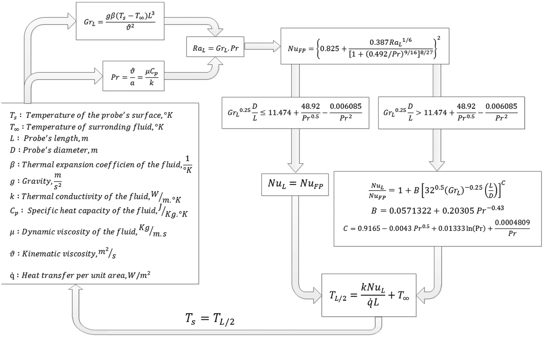
Process of determining the midpoint temperature of the probe by iteration.
Conduction
Fourier’s equation of heat conduction for a hot wire embedded in an infinite, homogeneous, isotropic medium can be solved as shown below 26
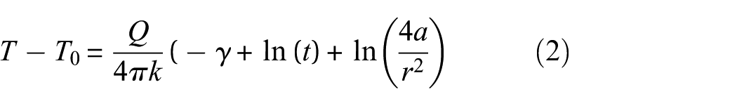
where
For a cylindrical probe of infinite length and radius R that has an infinite line source at its center and a contact resistance at the surface of the probe with heat transfer coefficient, H, the conduction equation was developed by De Vries and Peck. 27 Also, the heat transfer for a hollow cylinder, which is more complicated, has been solved. 18 These equations can be used in cases in which the geometry of the probe is different from a slender line heat source. However, these functions contain many variables, Bessel functions, and green functions, which are not easy to use. Despite the complexity of heat transfer in heat probes when the geometry of the heater is far from a hot wire, researchers have posited that it should be possible to use a relationship similar to that of the hot wire 28

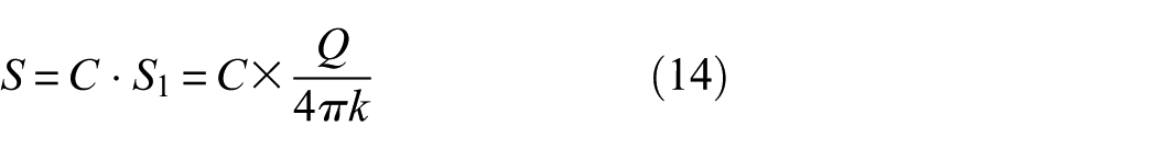
where the constants S and C are dependent on the thermal properties of the soil and the probe.
Numerical simulation of natural convection and conduction for the probe immersed in water and sediment
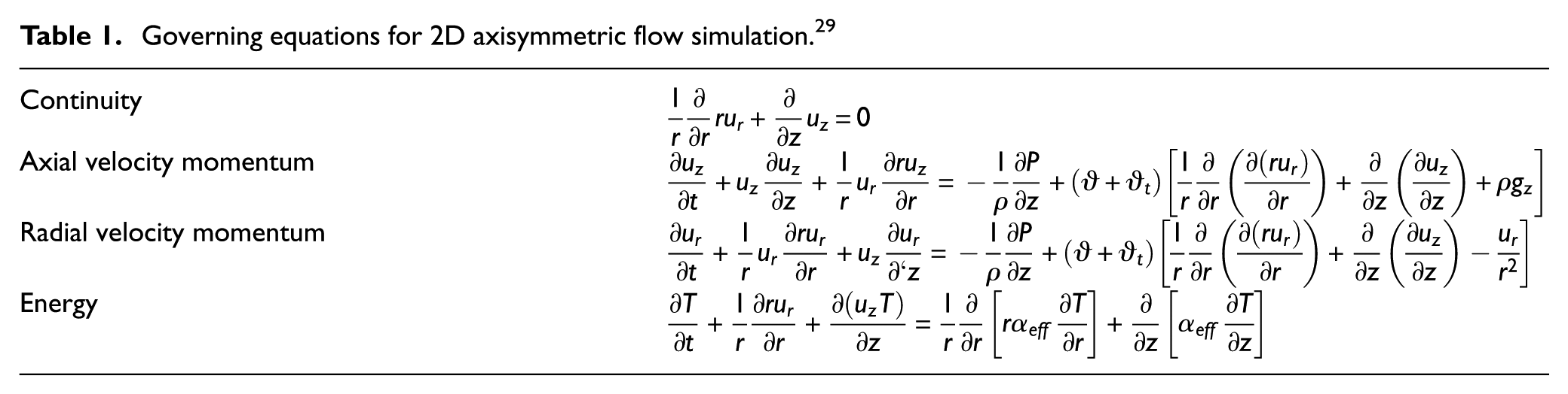
Natural convection and conduction can be modeled numerically. Continuity (mass), momentum, and energy equations 29 which are given in Table 1 are solved for single phase simulation. Fluent 6.3.26 was used to model natural convection inside the fluid and conduction inside the soil.
Governing equations for 2D axisymmetric flow simulation. 29
Method of solution
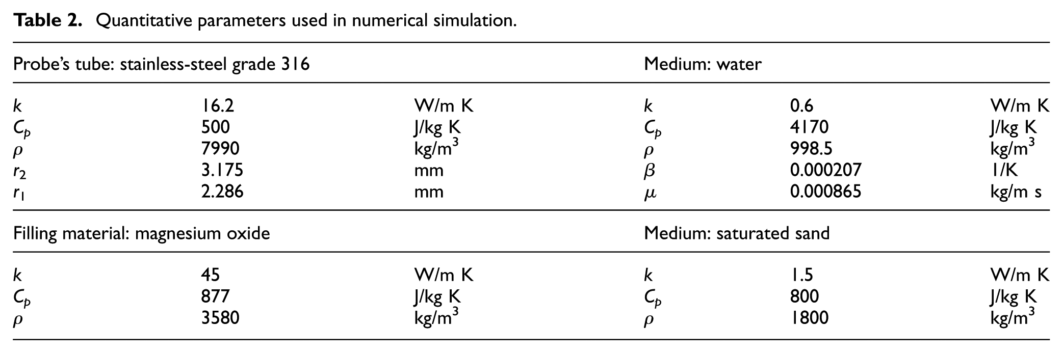
The computational work was done with Piso-Foam solver, and the second-order implicit scheme was used for time discretization. The software computes buoyancy-driven flows induced due to density changes in the fluid. The Boussinesq model was used for natural-convection flow. In this model, the density is constant in all equations except in the buoyancy term in the momentum equation, in which
Quantitative parameters used in numerical simulation.
Grid distribution and boundary condition
In this work, as an axisymmetric tank has been considered, only half of the geometry has been used for grid generation. A non-uniform grid was used, which was finer near the probe walls where gradients are more important than those away from the probe. As shown in Figure 2, the system consists of 3822 grids.
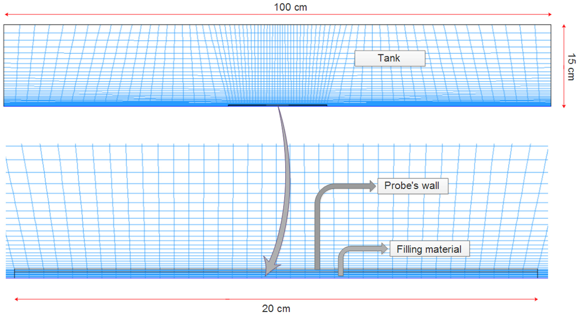
Schematic diagram of the grid for the probe immersed in water and sediment.
A constant temperature boundary condition has been given to side walls as well as top wall of the tank. Based on the established model, simulations were performed for the probe immersed in water and sediment. Figure 3 presents the contours of the simulated results for Q = 20 W/m.
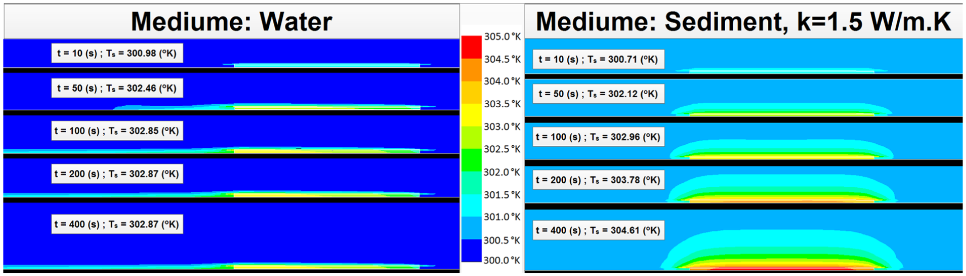
Contours of temperature field around the probe immersed in water and sediment for Q = 20 W/m.
Experimental tests
A sensor was fabricated that consisted of the following parts:
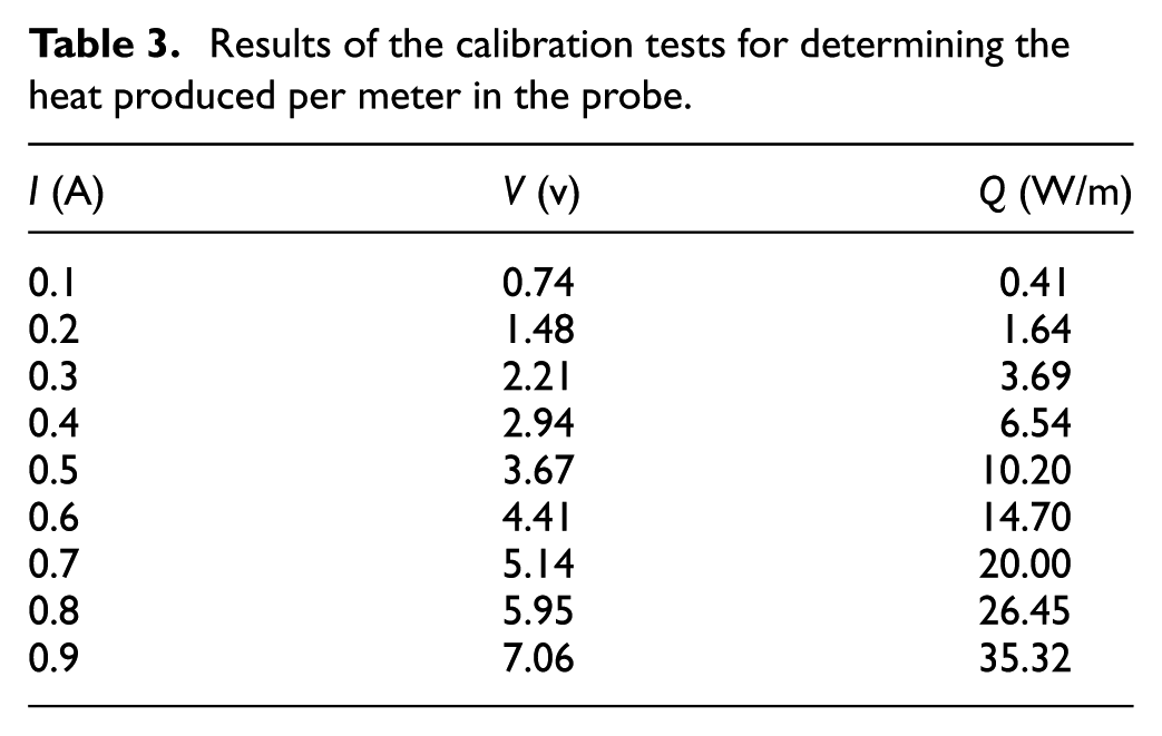
Heating wire: a high-resistance wire made of Kanthal A1 AWG-30 was used for heating the probe. The wire covered the probe’s length twice, and it was connected to a power supply unit. The resistance of the wire was measured in different currents, and the heat produced in the probe was calculated as shown in Table 3.
Thermistor: a negative temperature coefficient (NTC) thermistor with a resistance of 10 KΩ at 25°C was placed inside and in the middle of the probe. The resistance was collected by a data logger and sent to a PC, which converted the measurands to temperature values.
Probe: a stainless-steel tube with an outer diameter of 6.35 mm (0.25 in), a thickness of 0.889 mm (0.035 in), and a 20-cm length was used as the probe. The probe was filled with magnesium oxide. The end openings of the probe were sealed to prevent water from entering the probe.
Results of the calibration tests for determining the heat produced per meter in the probe.
The tests were conducted in the Hydraulics Laboratory at the University of Malaya, Faculty of Engineering. The tests were conducted in saturated soil and in water with the setup shown in Figure 4. The temperatures of the water and saturated sand were measured every 800 s.
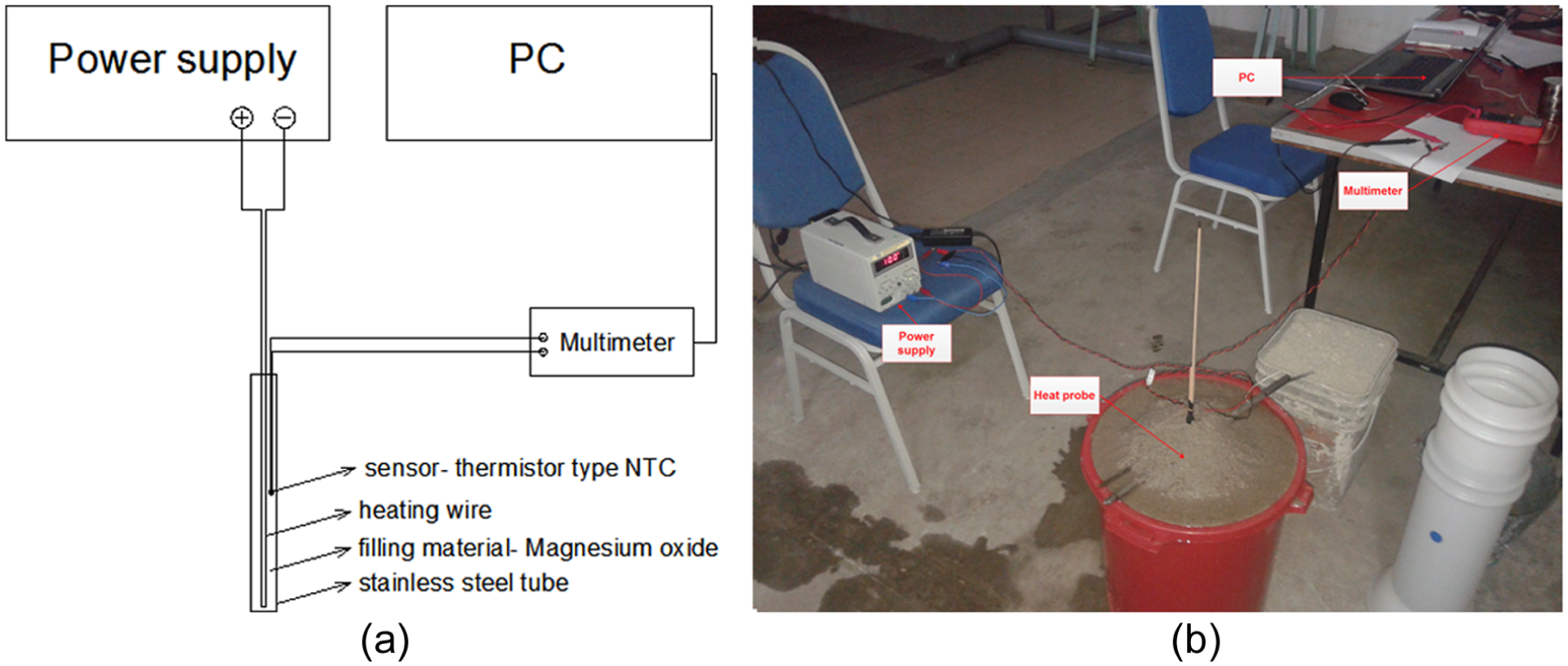
(a) Experimental setup: the heating wire and thermistor were placed in a stainless-steel tube, and the experimental setup consisted of the probe, a power supply, a data logger, and a PC. (b) Photograph of the experimental setup.
Results and discussion
The temperature difference in natural convection in water for the probe was calculated by mathematical analysis, Fluent simulation, and experiments. Figure 5 shows the results.
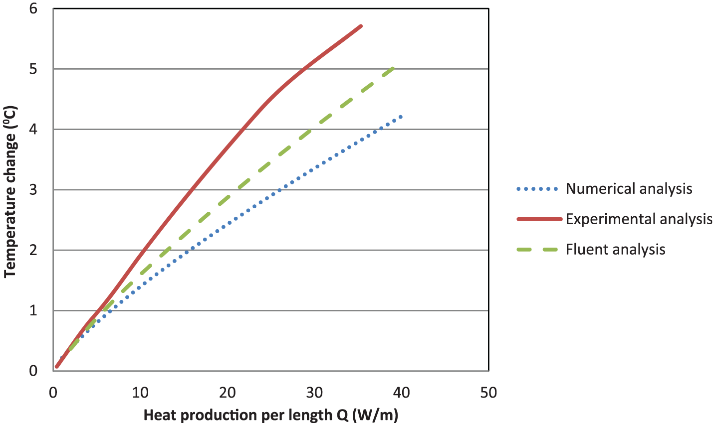
Temperature changes in the probe in water determined theoretically and experimentally.
Figure 5 shows that the experimental results did not agree completely with the results of the mathematical and simulation analyses. For natural convection, it can be seen that the sensor located inside the probe had a higher temperature than the temperature of the surface as predicted by numerical methods. The cause of this difference can be attributed to the following conditions:
The sensor was located inside the probe, so it detected a higher temperature than
There is a heat resistance between the filling material and the inner surface of hollow tube, the outer surface of the probe, and the medium (water). This resistance was not considered in the calculations.
The parameters used in the relationships were not exactly correct, and some parameters change with temperature, such as thermal conductivity, heat capacity, and the specific weight of water.
The relationships were based on fabricating the probe with the hot wire located exactly in the middle of the probe. However, because of the long length of the probe, this was not possible. Also, the sensor itself had volume, which affected the results.
The situation became even worse for the conduction phenomena. Figure 6 shows that the uncertainty of the thermal conductivity of the sediment resulted in different responses by the heat probe.
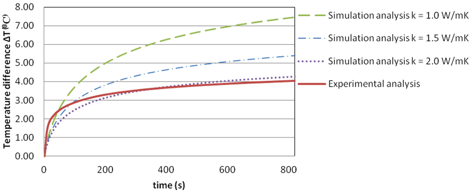
Heat probe response for Q = 20 W/m: experimental and theoretical results.
Despite all the differences between the simulations’ predictions and the experimental result, some methods can be used that can detect whether the probe is located in water or sediment. These methods use simple analyses and give us simple tools to deal with monitoring issues in water and sediment. Three methods have been developed for analyzing the data obtained from the heat probe.
S1: slope of ΔT-ln(t)
Heat transfer in saturated soil is based on conduction. Based on the theory of the infinite line source (also known as the hot-wire method), the change in the temperature is dependent on ln(t). Equation (2) shows that the slope of ΔT-ln(t) for the heating wire is
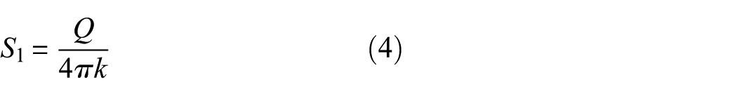
For the case of a large-diameter probe, the slope of ΔT-ln(t) is equal to
Heat transfer in fluids is based on convection. In that case, it can be said that after a time, the probe and medium reach a steady-state condition, and the slope of ΔT-ln(t) becomes 0. S was measured for different values of heat production (Figure 7).
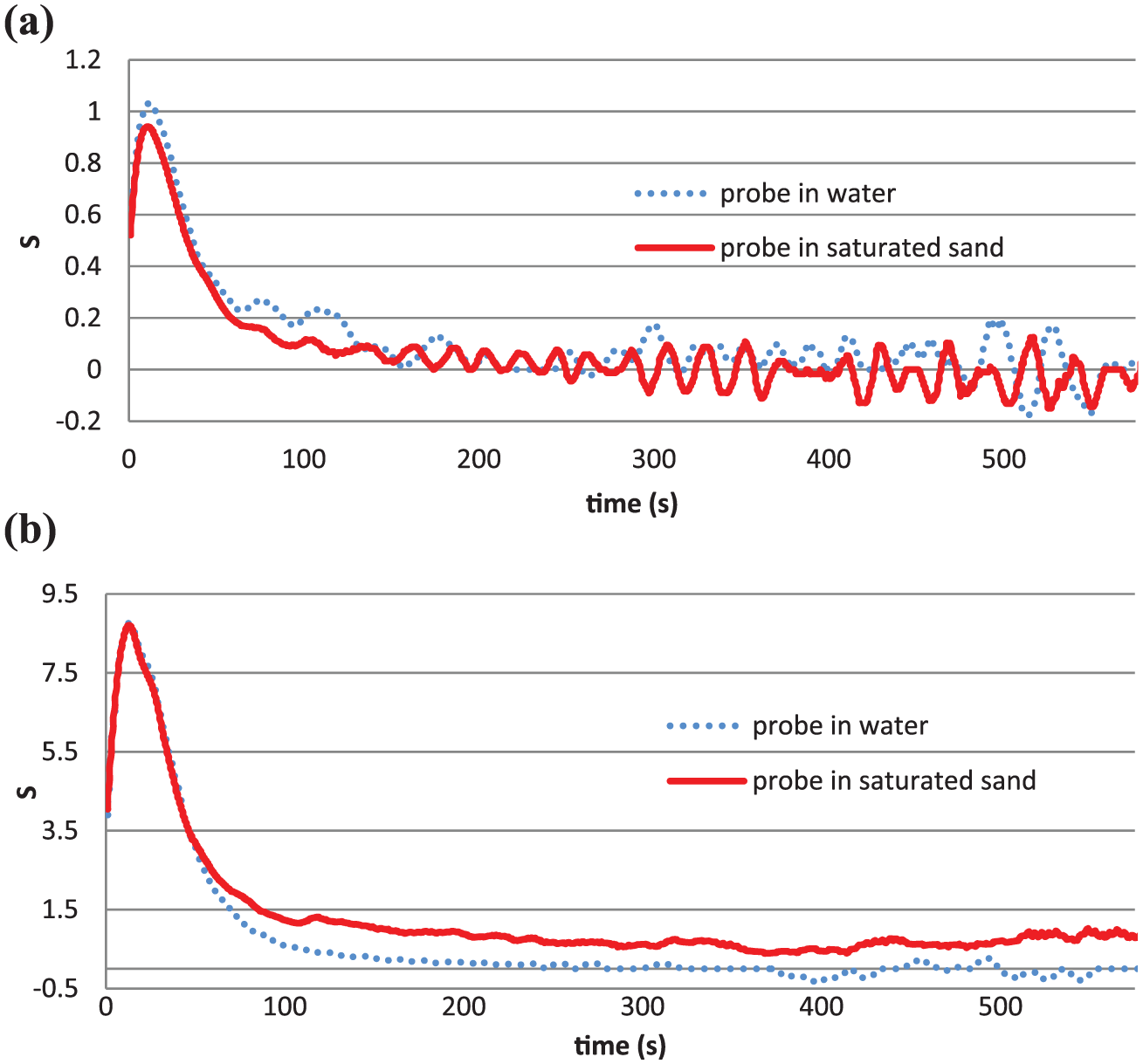
Variation of S (slope of ΔT-ln(t)) in water and saturated sand for (a) Q = 3.69 W/m and (b) Q = 20 W/m.
Figure 7(a) shows that for low heat production, S for saturated soil was very small and close to 0, so that heat is not appropriate for our purpose. In Figure 7(b), the value of S for saturated sand became about 0.6, and it was never less than 0.39. S became less than 0.39 after 129 s for water.
ΔΔT: temperature gap in water and soil
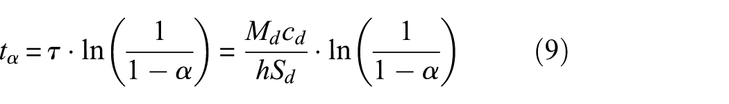
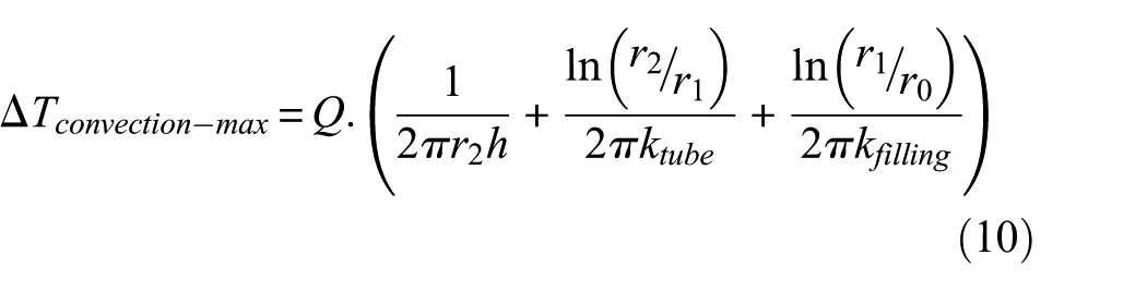
The conservation of energy law for a probe immersed in a fluid is
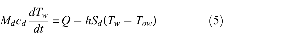
where
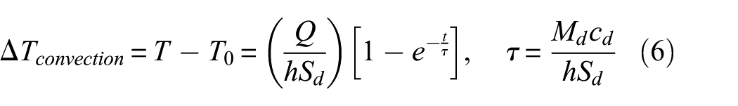
So, the temperature changes in water and saturated soil are different, and the difference can be determined by subtracting equations (15) from (10)
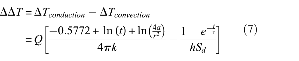
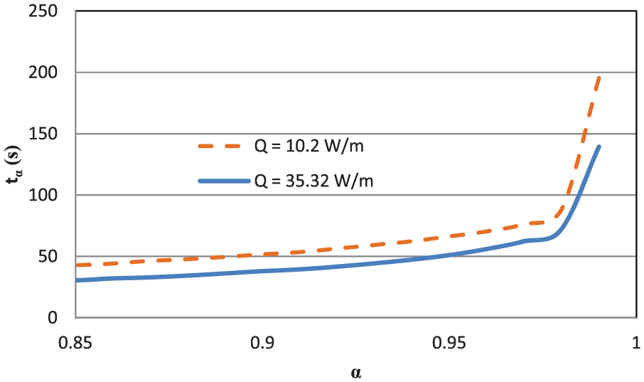
This method can be used for slender probes for determining proper system parameters, that is, power and time. Figure 8 shows the
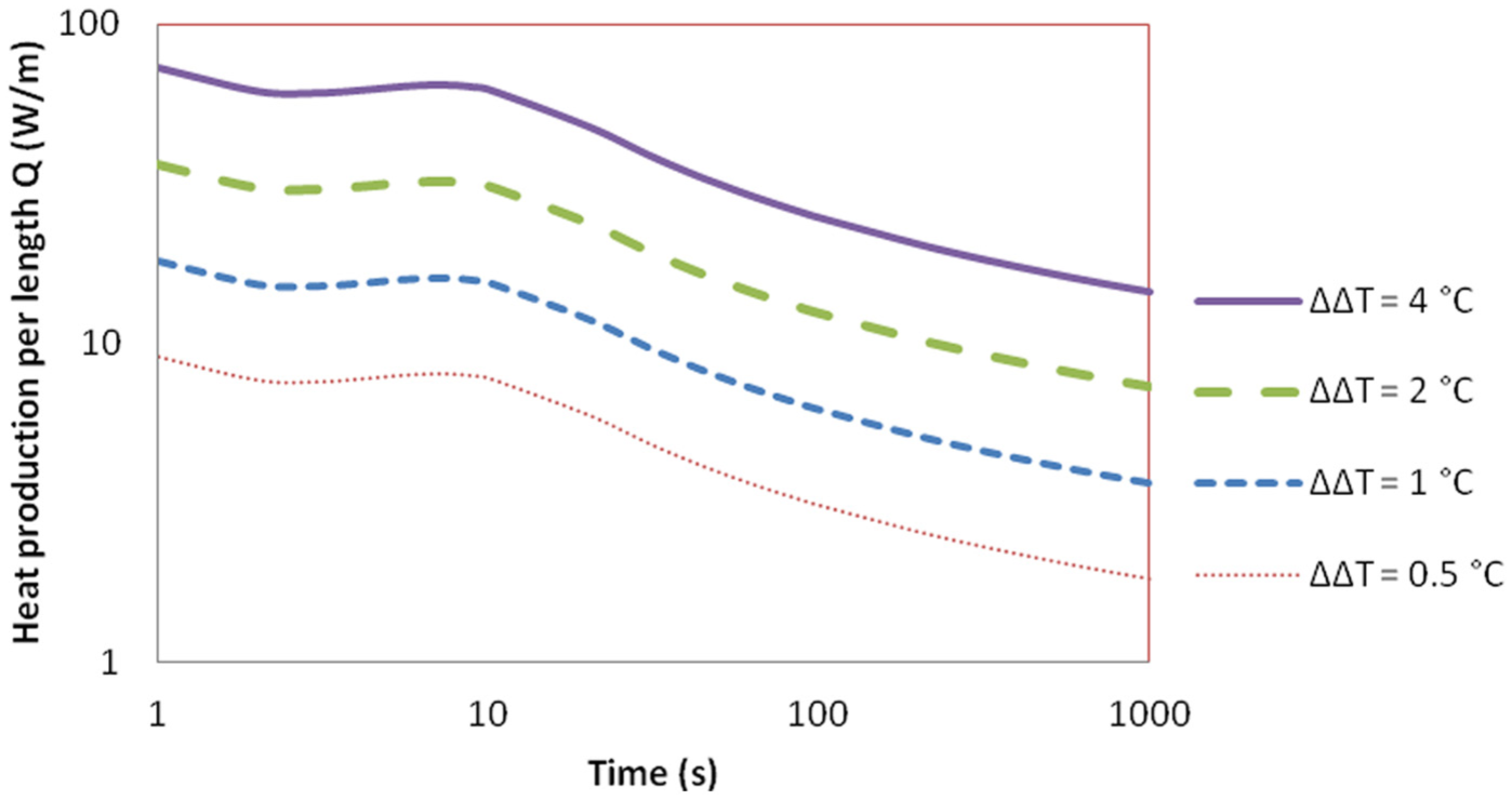
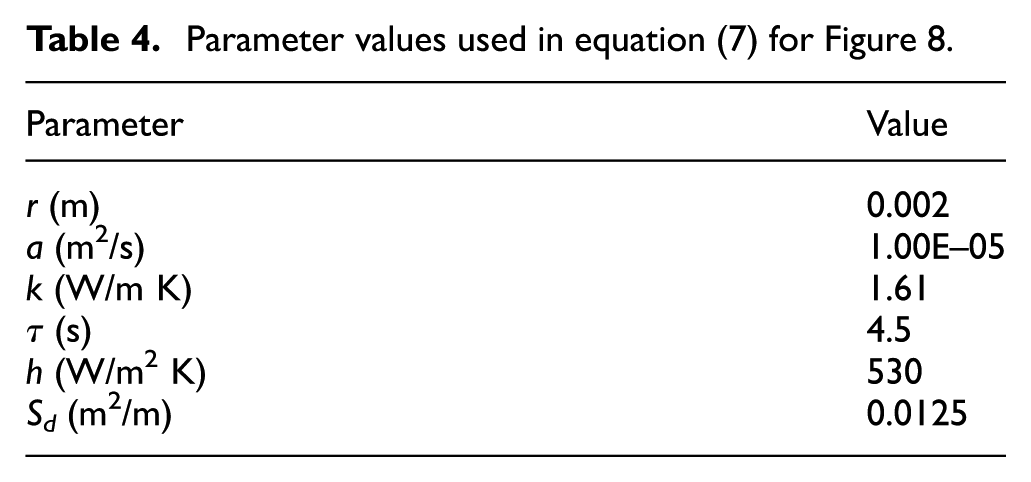
Parameter values used in equation (7) for Figure 8.
This method was used for a probe with a diameter of 3 mm, and the experimental results were superimposed on the contour lines in Figure 8 for time values more than 15 s.
30
Equation (7) is based on line heat theory and can be used for slender probes. Also, the parameters shown in Table 4 were not determined specifically. For example, by changing the thermal conductivity coefficient (k) from 1.61 to 2.5 W/m K, the counter lines moved upward considerably. Since the exact values of k and other parameters in Table 4 are unclear, choosing the appropriate values of Q and time in order to determine the best
: temperature comparison at
and
Calibration tests for determining
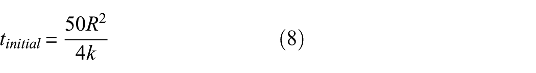
Reference 31 introduced a transient time for the measurement of conductivity, during which the sensor undergoes self-heating, and the change in temperature is influenced strongly by the sensor’s properties
For a hollow cylinder with inner and outer radii of
A similar method with an initial time
For example, by assuming
Since the methods are similar, the experimental results of the probe immersed in water can be used to calibrate the probe and to determine the value of
Values of
Figure 9 shows that the value of
Calibration tests for determining
The value of
where
Determining
The value of
Based on the definition of

For the probe located in sediment, based on equations (2) and (3), the value of temperature change due to conductive heat transfer is
So,
The values of
Comparison of temperature at
and
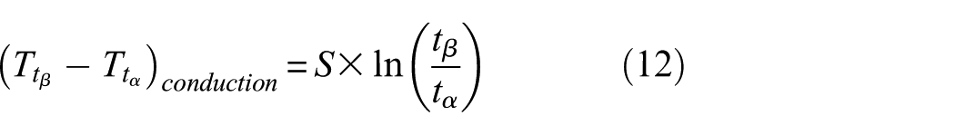
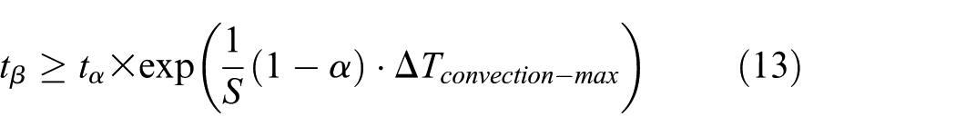
In this method, only the temperatures at two different times are measured, and if these temperature values do not satisfy equation (11), then it can be said that the probe is located in saturated soil. Using this method does not require continuous temperature measurements as is the case with the slope method. Also, the initial times, during which the behaviors of the probe in conduction and convection heat transfer were similar, were neglected.
For
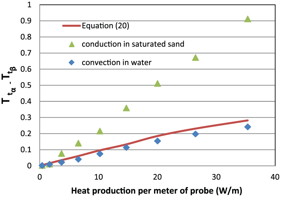
Experimental results of the sensor’s measurements located in water and saturated sand.
Figure 10 shows that if
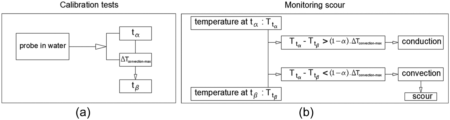
(a) Calibration and (b) scour-monitoring process using a large-scale heat probe.
In situ scour monitoring
The large-diameter heat probe is used to collect data from the field. The field data are analyzed by the method proposed in the previous section.
The Seri Setia Bridge that spans the Putrajaya River is located at the southeast of Putrajaya, Malaysia and consists of 8 spans of 30 m between pier centerlines. Each intermediate support consists of four flared piers. The large-diameter heat probe is installed on Piers P9 and P13 (shown in Figure 12).
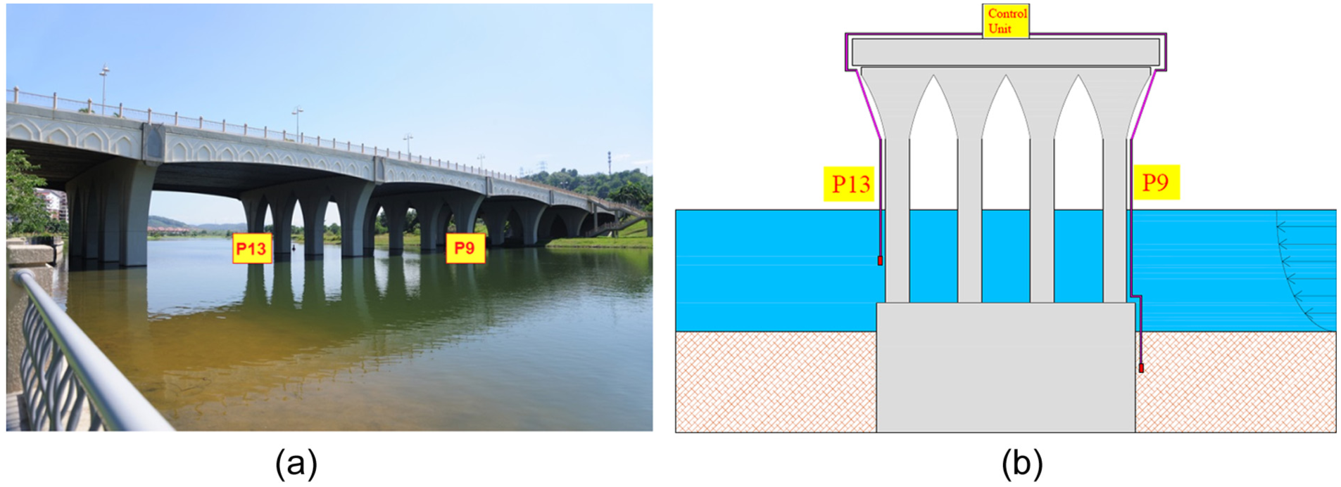
(a) Seri Setia Bridge piers P9 and P13 and (b) the layout of monitoring system.
Based on calibration tests, the values of
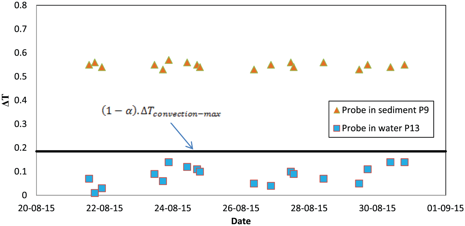
Temperature difference at
Conclusion
We studied the use of a large-diameter, hollow tube as a heat probe for monitoring scour. It uses the basic principle that the thermal properties of the two environments, water and soil, are different. Measuring the temperature showed that heat dissipation was different in this probe, depending on whether it was located in water or saturated sand. Three methods were introduced for analyzing results obtained from the probe. We studied the slope of the plot of ΔT versus ln(t), which requires continuous measurements over time. The
Footnotes
Declaration of Conflicting Interests
The author(s) declared no potential conflicts of interest with respect to the research, authorship, and/or publication of this article.
Funding
The author(s) disclosed receipt of the following financial support for the research, authorship, and/or publication of this article: This work was financially supported by the high-impact research grants from the University of Malaya (UM.C/625/1/HIR/61, account no. H-16001-00-D000061).