Monitoring fatigue-induced transverse matrix cracks in laminated composites using built-in acousto-ultrasonic techniques

Abstract

This work investigated the use of ultrasonic wave propagation in a composite laminate to monitor transverse matrix cracking. It was found that the change in the signal’s power spectral density correlates to crack density increase, and its sensitivity was dependent on the actuator to sensor orientation. This orientation dependence was found to be the same as that of the laminate’s stiffness degradation. A crack density damage index model was developed that relates signal changes to laminate stiffness degradation due to transverse matrix cracks. With this damage index model, a matrix cracking monitoring system was proposed, implemented, and validated. The developed system requires a calibration test for the composite layup of interest and a minimum of one actuator and two sensors at different angle orientations. The calibration test and general approach steps are described and validated. The system’s crack density estimates match experimentally measured crack density values within established error bounds.

Keywords

structural health monitoring system composite laminates transverse matrix cracking stiffness degradation piezoelectric sensors

Introduction

The use of carbon fiber–reinforced materials is increasing due to their superior properties of strength, stiffness, weight, performance, corrosion resistance, and so on. Their laminated construction is what allows the designer to tailor structural properties such as stiffness and strength to a given design while simultaneously reducing weight. But one of the major challenges with composite materials is that they suffer different damage types that can occur in sequence or simultaneously within different plies. Each failure mode or combination of these may have different impacts on the performance of the structure and makes damage inspection and monitoring very complex.^1,2 There are three main damage types: matrix cracking, ply delamination, and fiber breakage. Matrix cracking initiates first and promotes the development of the other damage types.

Much research has reported on methods to predict crack increase and ply degradation successfully.^1,3–9 If the amount of cracking could be monitored, then these damage models and damage tolerant strategies would be able to predict whether the laminate is close to failure or not. Current inspection practices for composites rely on nondestructive evaluation (NDE) techniques such as X-ray imaging, acoustic emissions, or C-scan techniques.^10,11 These NDE techniques, although efficient in damage detection, are not able to quantify crack density and are difficult and expensive to apply regularly since they require component disassembling, requiring the structure to be off-service.

Structural health monitoring (SHM) technology offers an alternative means to detect and monitor damage in structures in a fast and automated way. There are many types of SHM systems that can be used, but SHM systems based on piezoelectric sensors have been shown to be a very good method to create ultrasonic waves through composite structures.^2,12–16 Through the piezoelectric effect, piezoelectric disks can be used both as actuators and sensors. By actuating a permanently attached piezoelectric disk with a voltage input, the disk mechanically strains which causes an ultrasonic wave to propagate through the structure. When this wave reaches another piezoelectric disk in the structure, the disk strains and produces a voltage. Ultrasonic waves propagate through a medium with a phase velocity that is related to the plate’s material properties such as the plate’s stiffness and material density.¹⁷ These waves are dispersive and so they decrease with distance travelled.² Amplitude attenuation and energy losses do not have such a simple relationship to material properties and require finite element simulations of wave propagation.

Structural damage introduces discontinuities that will affect wave propagation. Via experiments and physics simulations researchers have observed that when waves interact with structural discontinuities, the waves reflect, scatter, and lose energy.^2,12 By introducing damage into the plate, the stiffness and damping of the plate is effectively reduced. Due to these structural discontinuities and degradation, the wave velocity, amplitude and energy will change with respect to the undamaged plate.

Most recent research has focused on detecting and locating damage, particularly delamination, holes, and simulated damage using scattered ultrasonic wave techniques.^2,13,18–25 Holes and delamination is localized damage within the structure that introduces a geometric discontinuity and scatters the propagated wave. On the other hand, matrix cracks are much smaller compared to delamination or holes, and they are distributed evenly within a composite plate. This damage type will not cause significant wave scattering, and hence the state-of-the-art damage monitoring techniques will not be able to monitor transverse cracking accurately. According to Su et al.’s² review of ultrasonic SHM techniques for composite structures, the wavelength of the propagated wave needs to be on the same order as the damage size for the damage to be detected, which translates to high frequency actuation. Smaller damage will not effectively cause any wave scattering but matrix cracking decreases the stiffness of composite laminates so it should affect wave propagation as well. Toyama et al.²⁶ and Seala et al.¹⁶ have reported results on the effect of matrix cracks on wave propagation, in particular how it affects wave velocity, but has not directly quantified matrix crack density.

Problem statement

Given sensor data, the desired output of a crack density monitoring system is total crack density. Hence, a monitoring methodology will be proposed and implemented so that the output of the developed monitoring system is total crack density for any given diagnostic path off-axis angle and laminate loading direction, as depicted in Figure 1.

Figure 1.

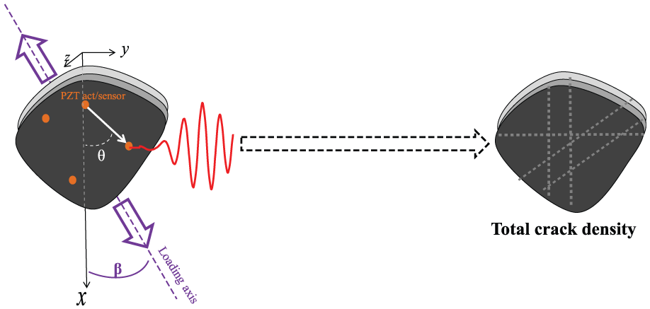
Schematic of objective and definition of off-axis angle θ and loading direction β. The dashed lines on the right figure depict the presence of matrix cracks.

Given a composite laminate with attached arrays of piezoelectric actuators and sensors and unknown load direction, the major goal of this research is to find how to relate the changes in sensor signal to total crack density. This relationship will enable monitoring the presence and quantity of matrix crack density.

Approach

The approach taken to achieve this goal has three main steps. The first step is to find a sensor signal feature that best correlates to crack density via experimental observation. The second step is to establish a robust relationship between this damage index (DI) and crack density using theoretical laminate stiffness degradation parameters. A schematic of these two steps is shown in Figure 2. The final step is to use this DI model to develop and implement a transverse matrix cracking SHM system. This monitoring method will be tested and implemented using a [90₂/45/−45]₂s notched laminates.

Figure 2.

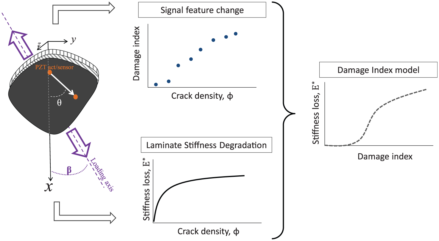
Schematic of approach and definition of off-axis angle and loading direction.

Laminate stiffness degradation due to transverse matrix cracking

The initiation, increase, and impact on ply stiffness of matrix cracking has been extensively studied and reported before.⁸ The model developed by Shahid and Chang⁴ has been chosen for the current work since it has been used previously and has been reported to match experimental observations. Given ply material properties, ply orientation and stacking sequence, the in-situ stiffness for each ply k can be computed for a given matrix crack density. Given a layup, the crack density at each ply is dependent on the direction of the applied load β. Ply stiffness as a function of cracking can then be used in Classical Lamination Theory²⁷ to compute the laminate effective stiffness $E_{x}$ when there is cracking in multiple plies and the off-axis angle θ varies.²⁸ The definitions of the loading direction β and off-axis angle θ are shown in Figure 2.

Laminate stiffness degradation $E^{*}$ is then dependent on total crack density $ϕ_{total}$ , the laminate’s off-axis angle $θ$ and the applied loading direction β. These semi-analytical results can be approximated by a Weibull cumulative distribution function (Weibull CDF), with the saturation and scale parameters P and g, respectively, dependent on β and θ

E^{*} = P (β, θ) (1 - \exp (- (\frac{ϕ_{total}}{g (β, θ)})))

(1)

Figures 3 and 4 show the results of implementing this stiffness degradation model to the two different layups at 0° applied load direction (β = 0).

Figure 3.

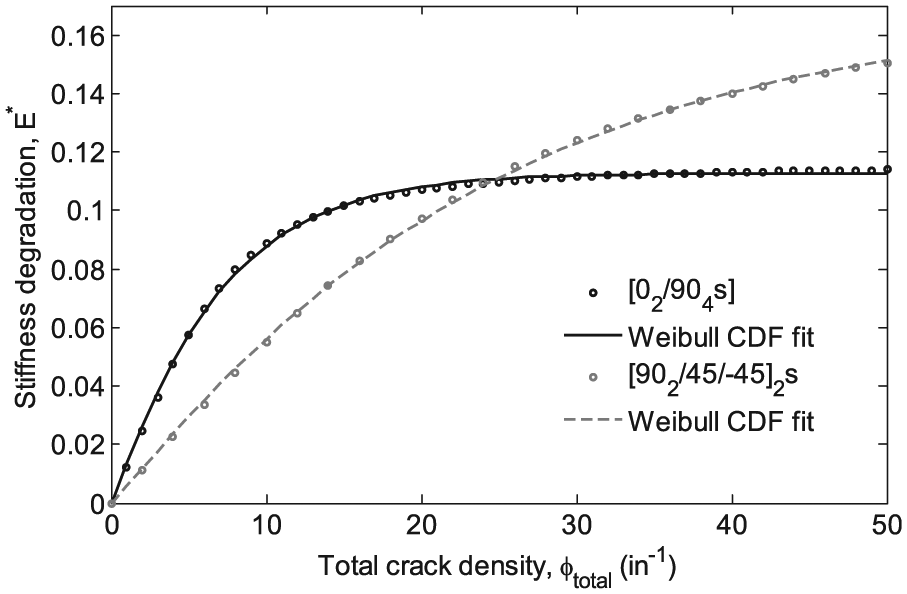
Stiffness degradation with crack density and Weibull CDF fit for zero off-axis and load direction.

Figure 4.

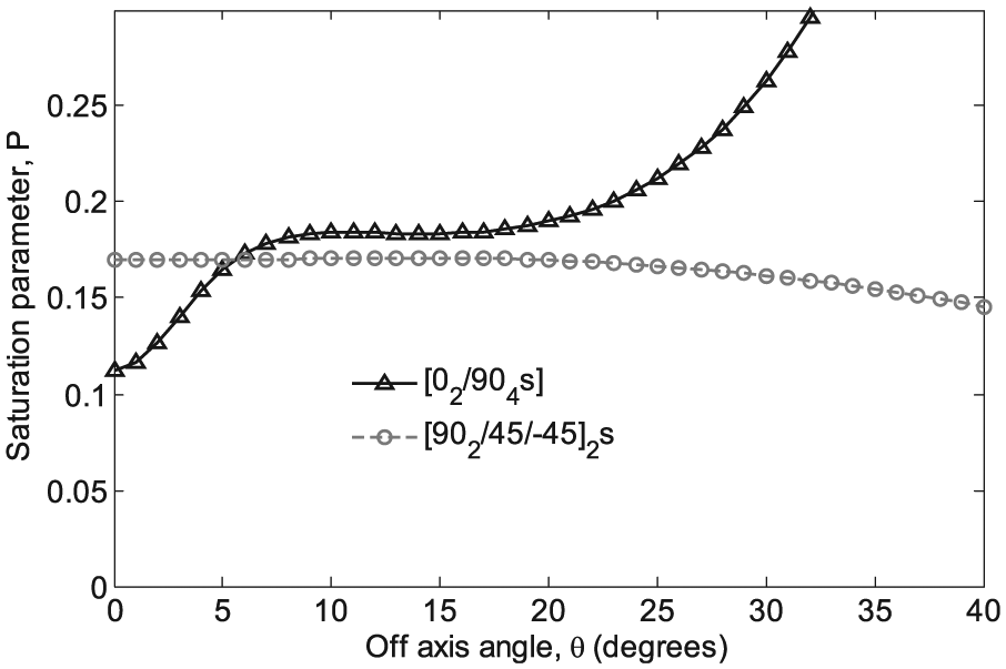
Saturation parameter P as off-axis angle changes for zero load direction.

Signal processing and feature extraction

The attached actuators and sensors propagate and receive ultrasonic waves, so it is possible to measure the changes on the wave parameters before and after damage has developed. These wave propagation changes are captured in the form of voltage changes as shown in Figure 4. There are many ways to analyze these voltage signals. Two common signal processing techniques are to analyze the signal in the time domain or in the frequency domain.² Saxena et al.²⁹ and Larrosa et al.^30,31 reported that time of flight (TOF), amplitude and power spectral density (PSD) were found to be sensitive to cracking as well as delamination. Following their findings, these three signal features will be analyzed in detail (Figure 5).

Figure 5.

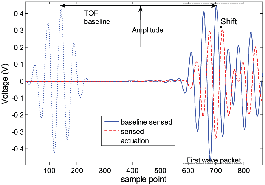
Example of actuation and sensed signals before and after damage for one diagnostic path.

The TOF and amplitude (A) can be computed from the sensed signal per diagnostic path in the time domain. The signal amplitude (A) relates to the amount of displacement caused by the propagating wave. Even though the relationship between amplitude and structural degradation is very complex, signal amplitude changes can be observed and are extracted from the time domain analysis as expressed by

A_{b} = \max (| b |)

(2)

Δ A = \frac{A_{b} - \max (| s |)}{A_{b}}

(3)

where b is the sensed baseline signal and s is the sensed signal after a cycle interval. The baseline data are the sensor signal acquired before the composite plate is tested. It represents the undamaged state.

The TOF is the time taken by an actuation signal to reach a sensor and is a measure of wave velocity. It is expressed by equation (4), where a is the actuation signal

TO F_{baseline} = t (\max (| b |)) - t (\max (| a |))

(4)

As the structure’s stiffness degrades, wave velocity decreases leading to increased TOF. The current signal’s normalized TOF is the baseline’s TOF plus the observed shift from the baseline, equation (5). The change in TOF, or shift, is estimated by cross-correlating current signal with baseline signal, equations (6) and (7)

Δ TOF = \frac{TO F_{baseline} + shift}{TO F_{baseline}}

(5)

R_{bs, s} (τ) = E [(b_{t} - μ_{b}) (s_{t + τ} - μ_{s})]

(6)

shift = t_{Total} - τ (\max (R_{b, s}))

(7)

The raw data can be decomposed into different frequency components via short-time Fourier transform (STFT), equation (8). Frequency domain features were extracted for the actuation frequency (ω) of 300 kHz after a STFT was performed, and the PSD was computed using equations (9) and (10)

STFT [S (n)] = S (m, ω) = \sum_{n = - \infty}^{\infty} s (n) w (n - m) e^{- j ω n}

(8)

PSD [S (n)] = P (m, ω) = k {| s (m, ω) |}^{2}

(9)

k = \frac{1}{F \sum_{n = 1}^{L} {| w (n) |}^{2}}

(10)

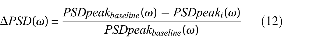
where S(n) is the signal, F is the sampling frequency, and m is the discrete size of the window w. And the power spectral density change ( $Δ PSD$ ) is computed as

Absolute PSD peak value

PSDpeak (ω) = \max (P (m, ω))

(11)

Normalized PSD change

Δ PSD (ω) = \frac{PSDpea k_{baseline} (ω) - PSDpea k_{i} (ω)}{PSDpea k_{baseline} (ω)}

(12)

DI selection criteria

Although delamination is important to monitor, the current goal is to find which feature best correlates to crack density so that delamination can be prevented. Once delamination has occurred, other damage monitoring techniques can be used such as the one developed by Ihn and Chang.¹⁹

The extracted features described above could exhibit different trends as transverse cracks increase and delamination develops, depicted in Figure 6. Feature 1 is sensitive to cracks but its sensitivity does not show a clear or smooth trend. Feature 2 is not very sensitive to cracks but is highly sensitive to delamination. On the other hand, feature 3 exhibits a smooth and clear trend with crack density increase but it is also sensitive to delamination. In this theoretical example, feature 3, although sensitive to delamination, it is highly correlated to cracks before delamination appears evidenced by its higher slope as cracks increase. This exercise help build a feature selection criteria to be used for experimental observations; the feature should behave smoothly and exhibit a high slope as crack density increases before delamination develops.

Figure 6.

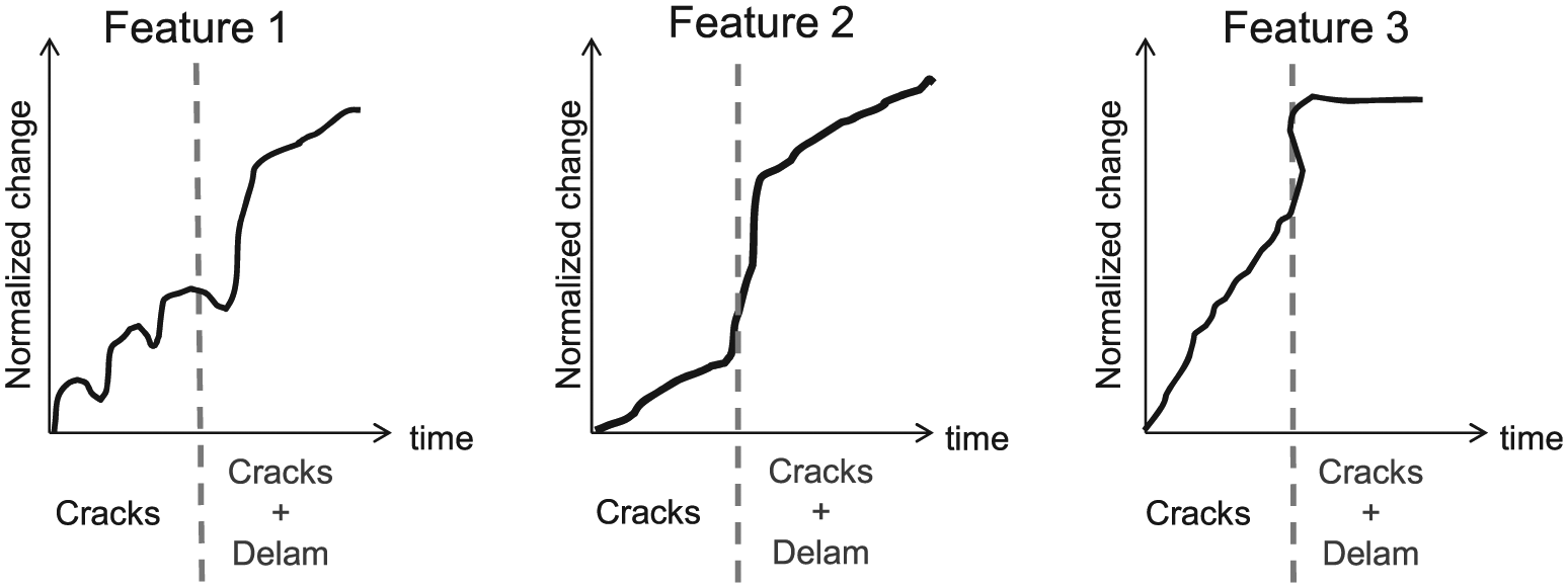
Theoretical feature behavior with different damage types.

Experimental details

Static and fatigue tests were conducted to observe how ultrasonic wave propagation changes as damage develops and increases in a composite laminate. Each composite sample was instrumented with 36 piezoelectric sensor/actuators and 3 strain gage rosettes. X-ray imaging of the composite samples was taken at different points in time to observe and quantify damage. The following sections describe in detail the materials used and testing procedures followed.

Composite samples

Three different layup configurations were tested during this study. Toray CA T700G/2510 unidirectional carbon-prepreg material was used. The composite laminates were vacuum bag and oven cured, and water-jet cut to specification by Composites Universal Group. According to the manufacturer’s specifications sheet, the laminates will have a void content of 5–7%. This void content will introduce some variability to the experimental results but since this material and manufacturing process is commonly used for aircraft parts, it was deemed adequate for implementation purposes. Glass tabs of approximately 2 in were attached to the top and bottom of each sample for clamping purposes during testing.

The layup configurations were chosen so that a variety of laminate damage mechanics behaviors could be observed. The layups to be tested are [0₂/90₄]s cross-ply laminates, [0/90₂/45/−45/90]s quasi-isotropic laminates, and [90₂/45/−45]₂s. Two geometries were used for the cross-ply samples: unnotched and notched geometry. The dimensions of these two different geometries are shown in Figure 7. The unnotched samples will develop matrix cracking only whereas the notched samples will have a combination of matrix cracking and delamination, which will help characterize the effect of these two damage types on ultrasonic wave propagation. Tests for the [0/90₂/45/−45/90]s and [90₂/45/−45]₂s layups were performed on notched samples only.

Figure 7.

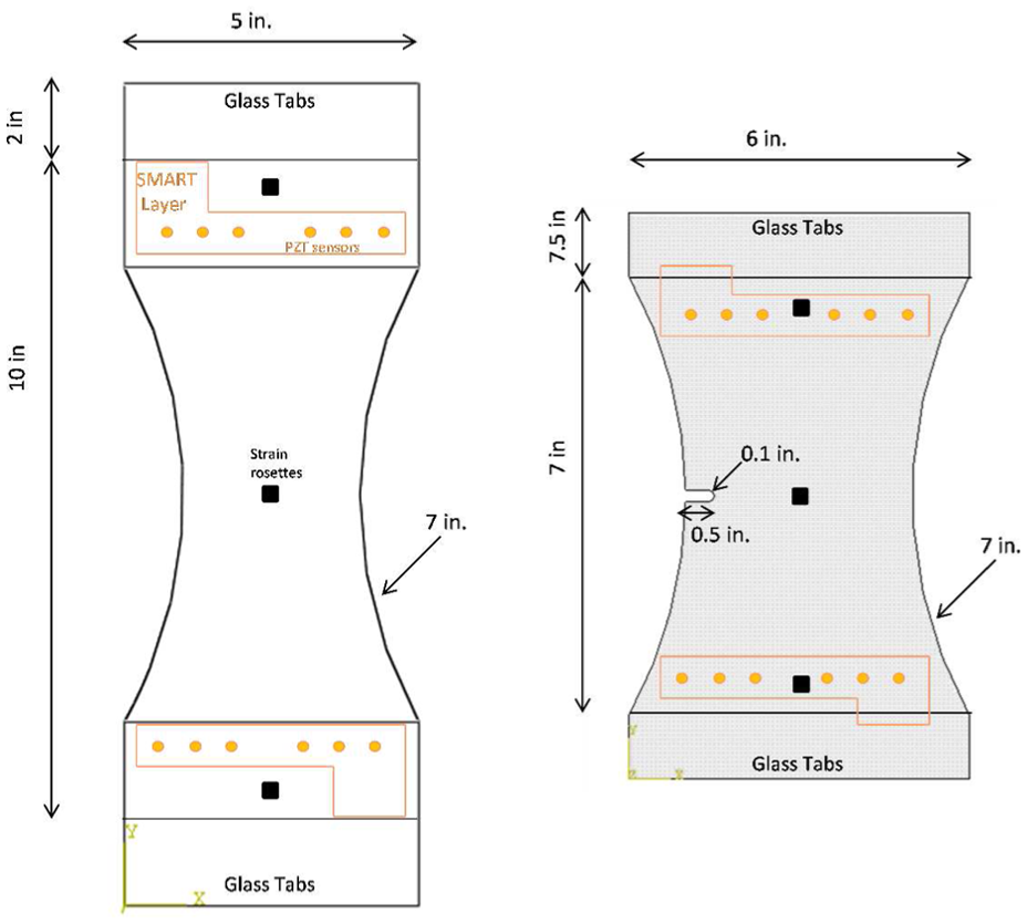
Unnotched and notched sample geometry and sensor placement.

Fatigue tests

The composite samples with attached sensors and actuators were subjected to tension–tension cyclic loading using an MTS universal testing machine. All tests were performed following ASTM Standards D3039 and D3479.^32,33 Using an MTS machine, samples were gripped using hydraulic grips, as shown in Figure 8.

Figure 8.

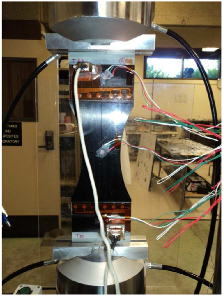
An unnotched cross-ply sample loaded in the MTS machine.

In order to design the fatigue tests, the static failure strength of each layup configuration was tested for two or three samples of each layup. Once the static failure strength was known, the maximum fatigue load was set to 70%–80% of the static failure strength, with a load ratio (R) of approximately 0.14. The fatigue tests followed a sinusoidal load profile at a frequency of 5 Hz.

The objective of the experiments is to be able to acquire sensor data as a function of damage progression, which can be obtained from X-ray images. The fatigue tests were stopped periodically to unload the sample from the testing machine. During unloading strain gage data was recorded. Once the sample was unloaded piezoelectric sensor data and X-Ray images were acquired.

Piezoelectric sensor network

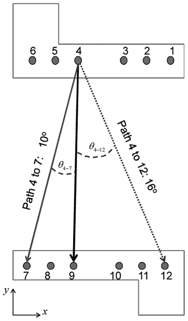
Two six-lead zirconate titanade (PZT)-sensor SMART Layers^® from Acellent Technologies were attached to the surface of each sample. This configuration provided six actuators and six sensors to monitor wave propagation through the samples (see Figure 9). Each of these sensors and actuators are 0.25 in diameter disks and 0.007 in thick. A Hysol^® 9696 adhesive film of 0.0004 in thick was used to attach the SMART Layers. This adhesive was chosen since it is a standard aerospace grade adhesive which has fairly good fatigue strength and minimal degradation. All samples’ actuators and sensors SMART Layers were placed 4 and 3 in away from the center of the unnotched and notched samples, respectively. Other information needed such as diagnostic path length and path’s angle with the sample’s long axis was calculated from the actuator and sensor coordinates. The actuator and sensor coordinates with respect to the samples bottom left-most corner were measured and recorded for each sample. Figure 9 shows a schematic with the sensor numbering and three examples of diagnostic paths with different angles. Piezoelectric sensors 1–6 were used as actuators and piezoelectric sensors 7–12 were used as sensors.

Figure 9.

Actuator and sensor configuration.

Acellent’s ScanScentry^® 32-channel data acquisition hardware and SmartPatch^® interface software were used to actuate and receive the corresponding signals for the 36 actuator–sensor paths. The input actuation was chosen to be a 5-peak burst signal at an actuation frequency range of 150–450 kHz, with an average input voltage of 50 V and a gain of 20 dB. The dispersion curves for the composite plates were computed using Disperse^® software. The frequency chosen was 300 kHz in order to have the fundamental symmetric and anti-symmetric modes as distinguishable as possible.

Diagnostic paths that lay close to edges were ignored since edge reflections introduced significant variability. Note that because the samples are relatively small, it is hard to distinguish the fundamental S₀ and A₀ modes from edge reflections; therefore, the current work will focus on the first wave packet of the received signal, see Figure 4.

Strain gages

As part of the study, it was of interest to gather strain information as damage increases. This information would be valuable for future finite element analysis validation as well as to monitor the local stiffness reduction as different damages develop and increase. Due to the asymmetry of the samples, three strain rosettes were placed on the samples as shown in Figures 7 and 8. The KFG strain rosettes were purchased from OMEGA.com; they are rated at maximum strain of 5%. The strain rosettes were attached to the samples’ surface using LOCITE 1-min cure adhesive.

X-ray imaging

Because damage develops between plies of the laminate, visual inspection for damage type is not possible, so X-ray of the samples was taken periodically. X-ray images of the samples were taken using a Faxitron X-ray cabinet. In order to be able to differentiate different damages in the composite sample, a dye penetrant (1,4 diiodobutane) was used to enhance X-ray absorption. Sensor signal was acquired before and after applying the dye penetrant. The dye penetrant was observed to affect signal, so the samples were exposed to 80° for an hour after each X-ray, and sensor signal acquired to check that the dye had completely evaporated. Figure 10 shows an example of an X-ray image of a notched cross-ply sample after 50,000 cycles. The bright white areas denote delaminated interfaces whereas the horizontal white lines are matrix cracks.

Figure 10.

X-ray of a notched cross-ply sample after 70,000 cycles.

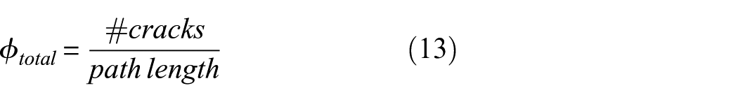
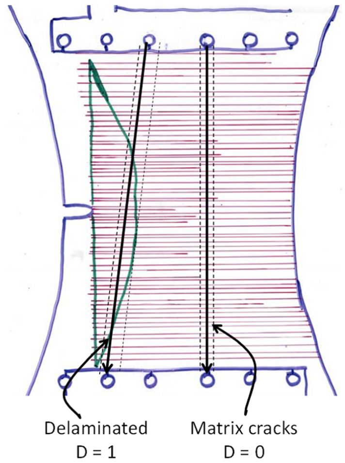
Once a sample was exposed to X-ray radiation, the film was processed in a dark room using a film developer. One of the issues with this analog process was that digitizing the X-ray film through a traditional scanner did not always result in clear images. So the damage in the film was traced using a marker over a transparency film. Each X-ray at each cycle interval was analyzed per diagnostic path zone. First each path zone was assigned a damage type (D) value of 0 if no damage or matrix cracks only had developed, or a damage type value of 1 if the path zone went through a delaminated area, as depicted in Figure 11. For the path zones that had developed matrix cracking, matrix cracks were manually counted and matrix crack density computed following equation (13). Since the X-rays only provide a 2D image of the cracks regardless of which ply has cracked, the amount of cracks is considered a thru thickness average of cracks

ϕ_{total} = \frac{# cracks}{path length}

(13)

Figure 11.

Transparency of a notched cross-ply sample after 40,000 cycles.

Experimental results

Three samples of each layup and geometry were tested and used for the current study. Each laminate developed damage differently.

The unnotched [0₂/90₄]s cross-ply laminates developed transverse cracks that spanned the entire sample’s width. The cracks increased up to a saturation value of 10 cracks/in. Small edge delaminations developed after 50,000 cycles. Test on unnotched samples was stopped after 500,000 cycles since there was no observable damage growth. The notched [0₂/90₄]s cross-ply laminates experienced delamination from the notch at the first cycle, with a fast growth rate up to 60,000 cycles at which point delamination growth was very slow, and tests were stopped after 150,000 cycles. Matrix cracking developed first by the notch, with cycles these cracks expanded through the samples’ width. As more cycles were introduced more and more cracks were formed up to a saturation of 11 cracks/in.

Matrix cracking and delamination for the [0/90₂/45/−45/90]s quasi-isotropic laminate was observed to develop and grow at the same rate. Delamination also developed at the notch at the very first cycle. In this layup, matrix cracking did not grow through the samples’ width and increased at a similar rate as with delamination. Matrix cracking did not reach saturation. Delamination grew fast up to 60,000 cycles, but afterwards damage growth was very slow, so testing was stopped around 200,000 cycles.

The [90₂/45/−45]₂s layup developed matrix cracking at earlier stages of loading. With cycles, cracks expanded through the width very quickly. Cracking saturation of 10 cracks/in was reached at 1000 cycles, at which point delamination developed by the notch. Delamination growth was very fast, which resulted in sample failures after 150,000 to 300,000 cycles.

At the conclusion of fatigue testing, each sample’s sensor data were processed into its corresponding features and the X-ray images analyzed into damage type and quantity. All this information for each diagnostic path at each cycle interval was merged so that signal changes as damage develops can be investigated.

DI selection

Detailed observation and analysis of the experimental data provided insight on how each feature behaves as damage develops, its repeatability and variability as off-axis angle and layup changes. Figure 12 shows a typical example of how the three features being investigated behave with damage development for a given sample. A general trend was observed where matrix cracks shift the signal slightly, but when delamination develops the signal is shifted significantly. Even though the amplitude jump with delamination is not as clear, a similar trend was observed in the decrease of amplitude. PSD exhibits a smooth increase with transverse cracks, and a not so significant jump as delamination develops.

Figure 12.

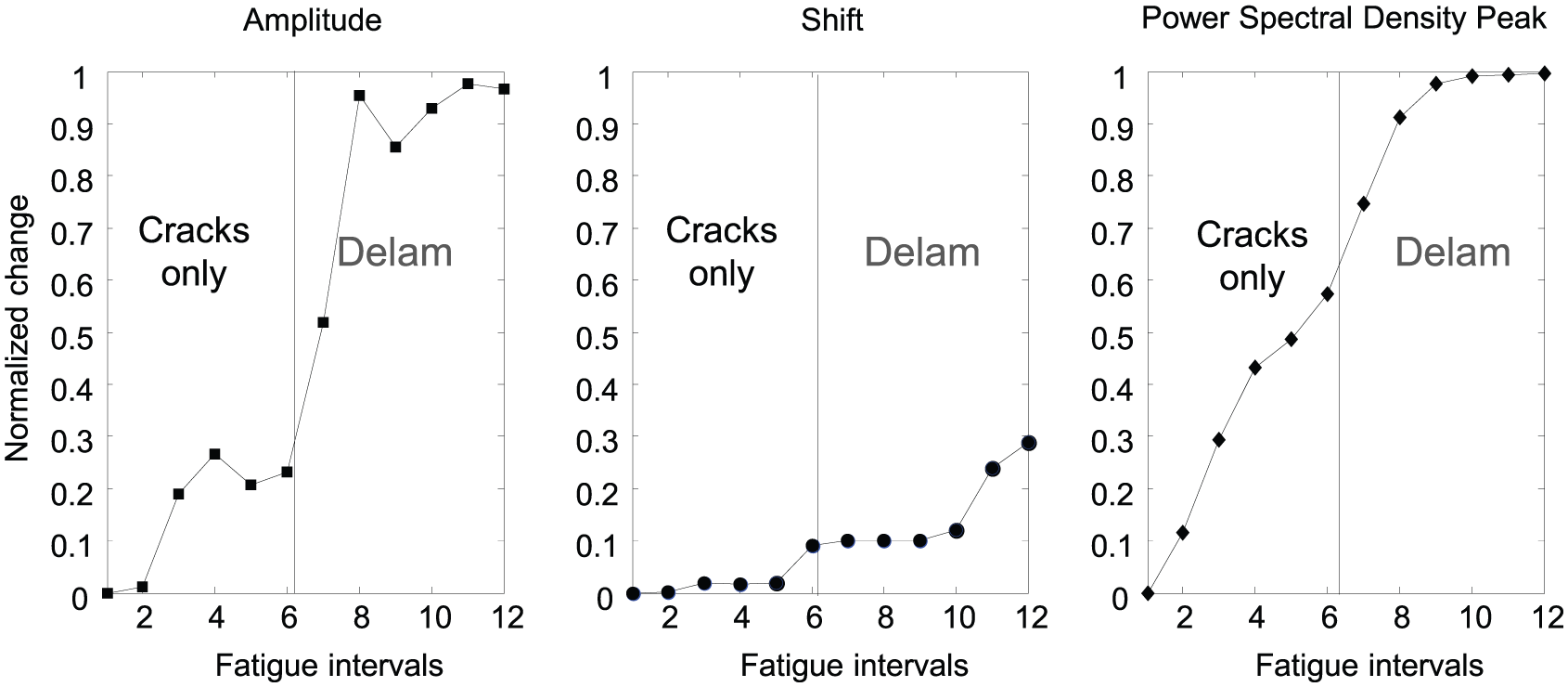
Example of how features change with damage development for a given sample and diagnostic path.

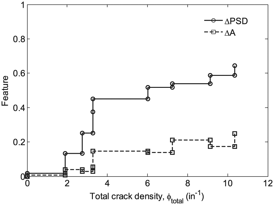
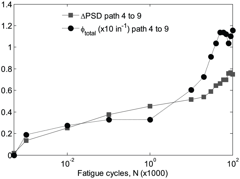
Detail observations revealed that amplitude (ΔA) and the PSD change (ΔPSD) features are correlated to matrix cracking while TOF showed to be more sensitive to delamination. The difference between amplitude and PSD is that PSD can be thought of as a filtered feature since it only contains information for specific frequency content, while amplitude is the product of multiple frequencies. Because of this, PSD change is more sensitive to matrix cracking than amplitude. Figure 13 shows a stair plot, or sensitivity plot, of PSD and amplitude change as matrix cracking increases. Note that PSD change with matrix cracking is more sensitive than amplitude change and it has a continuous increasing trend whereas amplitude changes oscillate. Furthermore, Figure 14 shows how matrix cracking and PSD change are increasing with cycles for a given diagnostic path. Both matrix crack density and PSD change have similar increasing trends, suggesting that they are highly correlated.

Figure 13.

Stair plots for PSD and amplitude change.

Figure 14.

PSD change and total crack density with fatigue cycles.

Following the feature selection criteria described previously, PSD change is the feature that best correlates to crack density for the three different layups tested. Hence, ΔPSD was selected as the crack density DI.

DI model

Now that PSD change has been chosen as the DI, the next step is to investigate how this DI changes with crack density. During the fatigue experiments, it was noted that unnotched cross-ply samples and [90₂/45/−45]₂s notched samples developed matrix cracking only and later in life delamination, but the quasi-isotropic samples developed matrix cracking and delamination simultaneously. Since the goal is to investigate the effect of crack density only, the quasi-isotropic samples will not be used in further analysis. In this section, the experimentally acquired PSD change data were analyzed as matrix crack density increases for the different diagnostic paths at different off-axis angles for the cross-ply unnotched samples only. The data gathered for the [90₂/45/−45]₂s notched samples will be used to test the robustness of the model and SHM system proposed.

It was observed that the PSD change is sensitive to the amount of matrix cracking and off-axis angle θ. Figure 15 presents PSD change as cracking increases for three paths of different off-axis angles. At low off-axis angles, such as 0°, the PSD change reaches a saturation point at which the increase of cracks does not affect it anymore. For higher angles, this saturation is not observed, but the trend is steeper and reaches high PSD change values at earlier crack densities.

Figure 15.

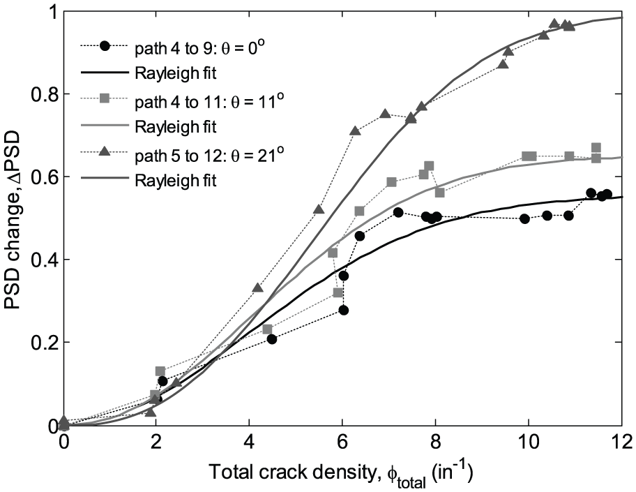
PSD change for different off-axis angles and corresponding Rayleigh fits for a [0₂/90₄]s sample.

Another important observation was that PSD changes with cracking follows a Rayleigh cumulative distribution function (Rayleigh CDF, equation (14)) regardless of off-axis angle, as depicted by the fitted curves in Figure 15

Δ PSD = B (θ) (1 - \exp (- {(\frac{ϕ_{total}}{d (θ)})}^{2}))

(14)

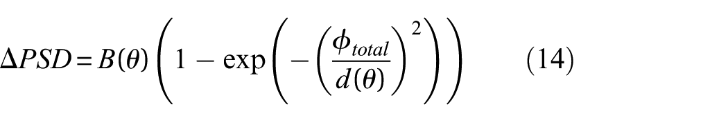
The Rayleigh CDF saturation and scale parameters B and d, respectively, were observed to depend on the off-axis angle. Note that the experiments were performed with loading direction at 0°, and hence, all data presented in the following sections are for $β = 0$ and varying $θ$ . The unknown parameters B and d can be found using least squares regression for each path’s experimental data. Using MATLAB^® regression, the optimum B, d and R² values for each path were computed. As an example, the results for three different paths at 21° from a sample of [0₂/90₄]s layup are shown in Figure 16. Although there is some variability for paths of the same angle, the B and d values for the same angles are very close. But as the off-axis angle changes, B and d are changing as well, as shown in Figure 17 for the scale parameter d.

Figure 16.

PSD change for different paths at off-axis angle of 21° and corresponding Rayleigh fits.

Figure 17.

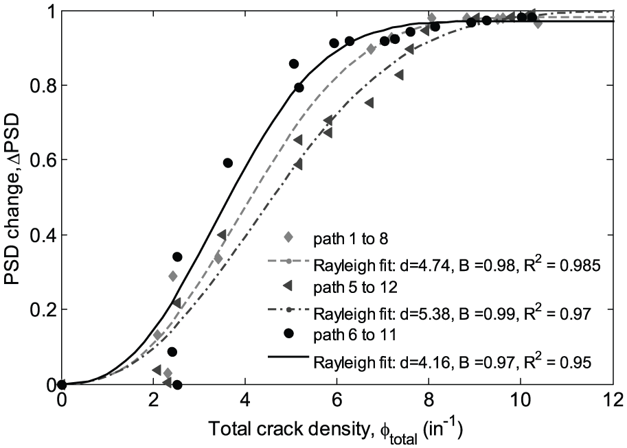
[0₂/90₄]s scale parameters d and g as off-axis angle changes. All data from unnotched cross-ply samples were tested.

The impact of matrix cracking on laminate stiffness was analyzed in section “Laminate stiffness degradation due to transverse matrix cracking,” and it was concluded that stiffness degradation can be described with a Weibull CDF that is dependent on the amount of cracking and the off-axis angle. A Weibull CDF is a special case of a Rayleigh CDF and it was observed that the general trend on saturation and scale parameters P, B, g, and d as angle changes was very similar. For comparison, the saturation and scale parameters for stiffness degradation were scaled by a constant and plotted with the experimental results to observe whether the dependence with off-axis angle was similar. Figure 17 shows the plot for d and g. Comparing the scaled Weibull theoretical parameters to the experimentally obtained Rayleigh parameters, it can be observed that the dependence with off-axis angle is the same. If the correct scalar constant is chosen, the scaled theoretical values lie within the experimental values’ variability.

These results suggest that the experimental Rayleigh parameters are linearly related to the stiffness degradation parameters. With this in mind, the experimental PSD change scale and saturation parameters were plotted against the theoretical stiffness parameter values, as shown in Figure 18. Using least squares regression, a linear fit can be found such that

B (θ, β) = m * P (θ, β)

(15)

d (θ, β) = n * g (θ, β)

(16)

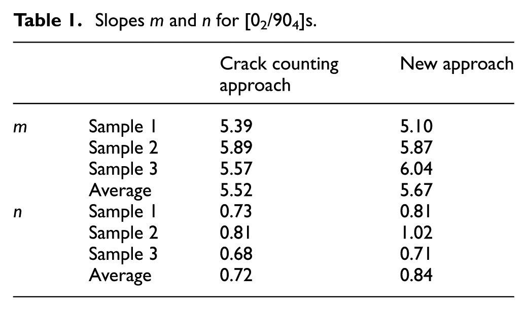
where m is the saturation slope and n is the scale slope of the linear relationship between stiffness degradation Weibull and PSD change Rayleigh parameters. Although other fits with higher order polynomials or other functions could be explored, a linear fit was chosen because of its simplicity and fairly comparable fit performance. The values estimated for the stiffness degradation to PSD change parameter slopes are shown in Table 1 under the crack counting approach column.

Figure 18.

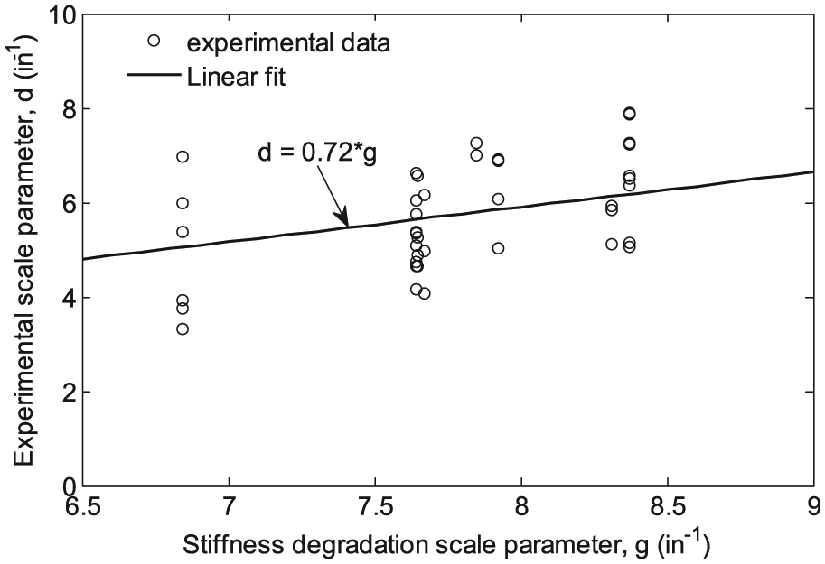
[0₂/90₄]s experimental versus theoretical scale parameters. All data from unnotched cross-ply samples were tested.

Table 1.

Slopes m and n for [0₂/90₄]s.

		Crack counting approach	New approach
m	Sample 1	5.39	5.10
	Sample 2	5.89	5.87
	Sample 3	5.57	6.04
	Average	5.52	5.67
n	Sample 1	0.73	0.81
	Sample 2	0.81	1.02
	Sample 3	0.68	0.71
	Average	0.72	0.84

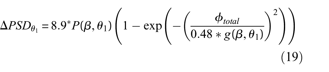
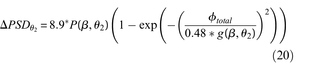
Substituting equations (15) and (16) into equation (14), we arrive at the following DI to crack density relationship

Δ PSD (ϕ_{total}, β, θ) = m^{*} P (β, θ) (1 - \exp (- {(\frac{ϕ_{total}}{n^{*} g (β, θ)})}^{2}))

(17)

where $P (β, θ) and g (β, θ)$ are obtained from the theoretical laminate stiffness degradation model and $m and n$ are the saturation and scale slopes found from experiments and are not dependent on the off-axis angle or loading direction.

DI model parameters: n and m

Although the methodology to find m and n described above is valid, this experimental procedure is labor intensive and very time-consuming; testing one sample took approximately 4 weeks. Taking X-rays required the testing to be stopped, the sample to be unloaded which increased the testing time and effort. Processing and analyzing the X-rays was very challenging, especially the manual crack counting. For these findings to be used in practical applications, a more robust and practical experimental approach needs to be developed to find $m and n$ for any material and layup configuration.

With equations (1) and (17) at hand and eliminating crack density, the DI model can be expressed as

E^{*} = P (β, θ) (1 - \exp (- n {(- \ln (1 - \frac{Δ PSD}{m * P (β, θ)}))}^{\frac{1}{2}}))

(18)

Experimental laminate stiffness degradation can be measured using the attached strain gages. The strain gages attached in the tested samples will only measure stiffness at 0°, 45°, and 90° off-axis angles, but the theoretical model provides stiffness estimates at any off-axis angle of interest. The SMART Layer used for these experiments restricts the PZT sensor data acquired to diagnostic path angles below 29°. Hence, the DI model for 0° off axis angle and 0° loading direction was compared to the experimental data acquired from the 0° strain gage and diagnostic path 3–10 data for all three unnotched cross-ply samples tested. Figure 19 shows the comparison for the unnotched cross-ply sample 1. The DI model follows the experimental trend and the model estimates lie within the experimental variability (as denoted by the error bars).

Figure 19.

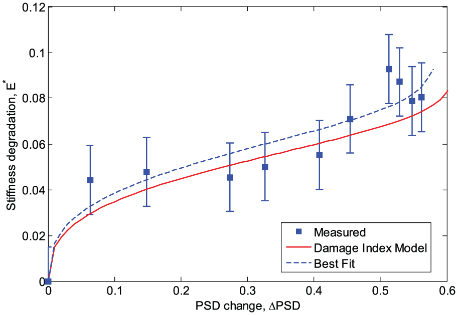
Stiffness degradation versus PSD change. Measured refers to stiffness degradation calculated from strain gage data. The dashed curve is the best fit to the measured data. The solid curve represents the DI model.

If one notes that equation (18) is not explicitly dependent on crack density, then this form of the DI model could be used for a more practical approach. If stiffness degradation values are known for certain PSD change, then the unknown parameters could be estimated via regression. As described previously, the stiffness degradation could be calculated experimentally through strain gage data alone (as opposed to estimating it using crack density values). Figure 19 shows a sample’s measured stiffness degradation via strain gages for different PSD change values for the unnotched cross-ply sample 1 and diagnostic path 3–10. These values were used to find the best fit to equation (18). The m and n estimates for the two different approaches are presented in Table 1. Comparing the new and previous approach, the new approach m and n estimates vary within 10% of the counting cracks approach estimates. These results demonstrate that the unknown m and n slope parameters for a given layup can be found experimentally without the need to know crack density.

In summary, the new and more practical testing setup, procedure, and data collection are as follows and are depicted in Figure 20:

Composite samples (either a necking or straight geometry) with desired material and layup configuration instrumented with:

Strain gage attached to measure strain in the direction of applied loading.

Attached sensors; one PZT actuator and one PZT sensor to measure wave propagation

Quasi-static tensile or tensile–tensile fatigue test stopping at different loading/cycle levels to capture strain and sensor data at early and mid-stages of matrix cracking

Post-process strain and sensor data into stiffness degradation and PSD change for each of the data collection intervals and plot stiffness degradation versus PSD change.

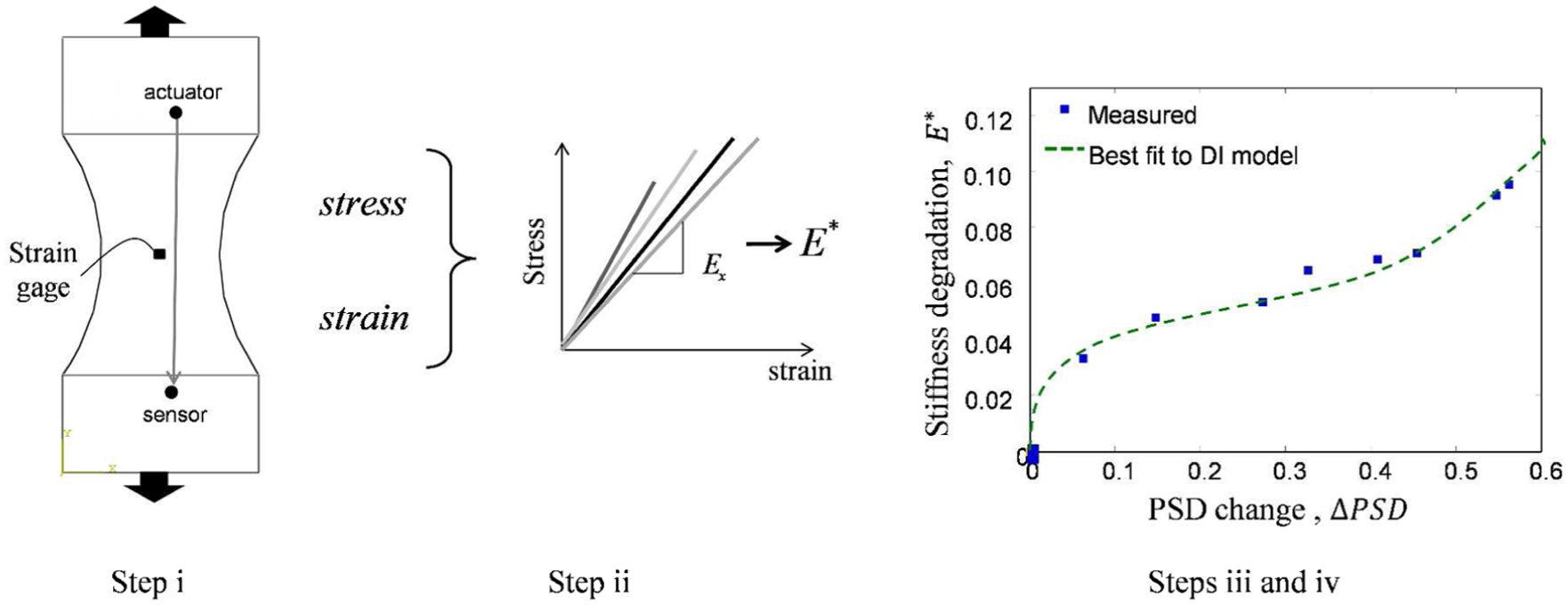
Using least squares or maximum likelihood regression, find the optimum $m and n$ values that best fit equation (18) and the data plotted in step 3. These are the saturation m and scale n slopes for the given layup configuration.

Figure 20.

New procedure to find the damage index model parameters m and n.

Transverse matrix cracking monitoring system

In an SHM application, the DI is known from the data provided by the attached sensors and the unknowns are total crack density and loading direction. Hence, it is desired to solve the inverse problem: if the DI is known, can total crack density be estimated?

Proposed method

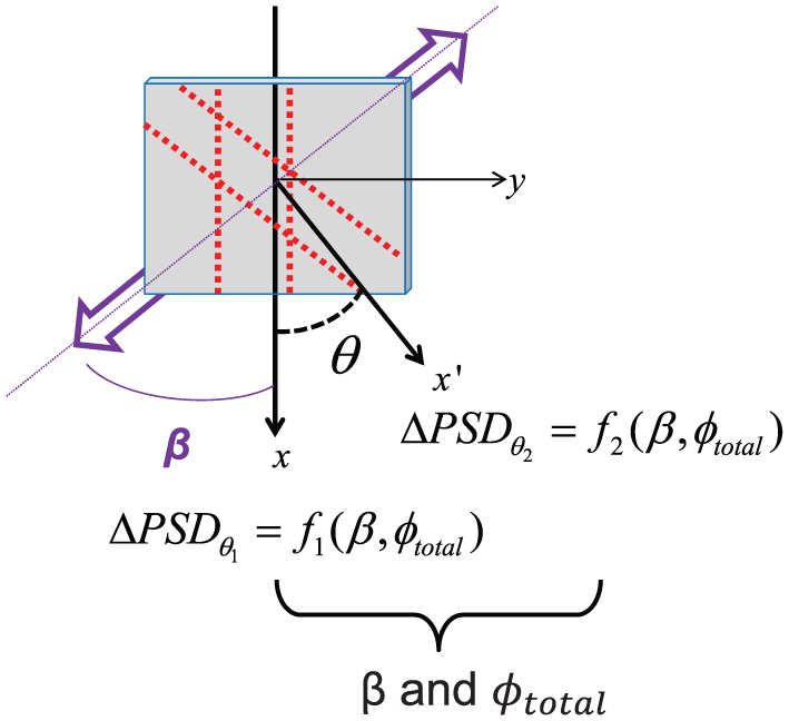
Since the DI to crack density relationship of equation (17) has two unknowns, $β and ϕ_{total}$ , two equations are needed to solve for these unknowns. The dependence on diagnostic path off-axis angle $θ$ provides two equations for the two unknowns. With two PSD change measurements at different off-axis angles, $Δ PS D_{θ_{1}}$ and $Δ PS D_{θ_{2}}$ , the system of nonlinear equations with two unknowns can be solved, as depicted in Figure 21. This indicates that two actuator to sensor paths would be enough to solve for crack density.

Figure 21.

Two signal measurements to solve for two unknowns. Bold arrows represent the loading direction; the dotted red lines represent matrix cracks.

The monitoring method proposed consists of six major steps, given layup stacking sequence and material properties:

Set up DI to cracking relationship, equation (17):

Run the theoretical stiffness degradation model to compute the functions $P (β, θ)$ and $g (β, θ)$

Calibration test using equation (18); to get the saturation and scale slopes (m and n) for the layup of interest

Implementation:

3. Attach a minimum of one actuator and two sensors,

4. Extract the DI: PSD change

5. Use the crack to DI scheme, as shown in Figure 21

6. If more than two sensor paths are available, apply a crack density diagnosis

Figure 22 presents the information flow of the developed crack density monitoring system. The major inputs to the system are sensed data from (at least) two actuator to sensor paths, unidirectional ply material properties, layup configuration and calibration parameters. With this information, the developed monitoring method will output an estimate of total crack density in the laminate.

Figure 22.

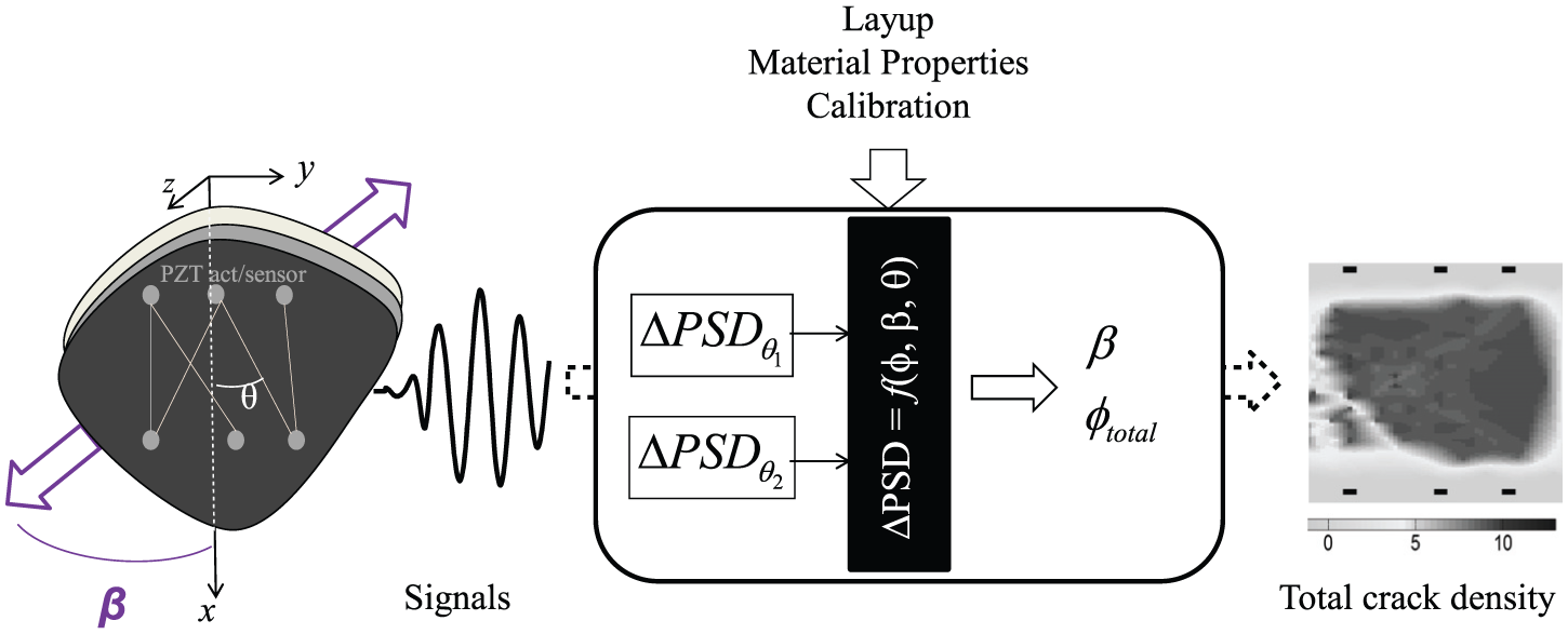
Crack density monitoring system.

Validation

In this section, a [90₂/45/−45]₂s layup constructed from Torayca T700G/2510 will be used to set up the crack monitoring scheme presented above. The calibration tests followed the procedure presented previously, and the optimum values for m and n were 8.9 and 0.48, respectively. The sample was instrumented with 12 piezoelectric disks: six actuators and six sensors. This translates to 36 diagnostic paths. Given that a sensor network may have different pairs of sensor paths, it is of interest to test how the crack density monitoring model performs with pairs of different off-axis angles. For validation purposes only, two diagnostic paths will be used to compute loading direction and total crack density. Six different path pairs were tested for this sample ranging from 7° to 35° apart. The paths tested are shown in Figure 23. Note that paths close to edges are not used because wave reflections will introduce significant variability.

Figure 23.

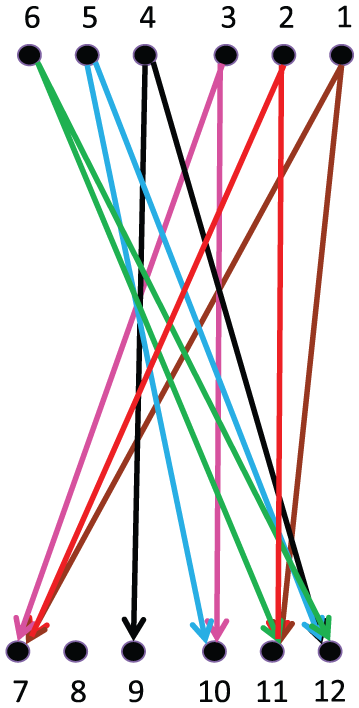
Six different pairs of paths used for validation.

The DI was selected to be the PSD change as previously described and was extracted at the actuation frequency of 300 kHz. Each time, sensor data were acquired, ΔPSD was extracted for each diagnostic path as described above, and an X-ray of the sample was taken to experimentally measure total matrix crack density. Each path pair was then used separately to solve for the loading direction and crack density as follows

Δ PS D_{θ_{1}} = 8 . 9^{*} P (β, θ_{1}) (1 - \exp (- {(\frac{ϕ_{total}}{0.48 * g (β, θ_{1})})}^{2}))

(19)

Δ PS D_{θ_{2}} = 8 . 9^{*} P (β, θ_{2}) (1 - \exp (- {(\frac{ϕ_{total}}{0.48 * g (β, θ_{2})})}^{2}))

(20)

$θ_{1}$ , $θ_{2}$ , $Δ PS D_{θ_{1}}$ , and $Δ PS D_{θ_{2}}$ are all known. These set of equations were solved using the fsolve function in MATLAB, to solve for $ϕ_{total}$ and $β$ .

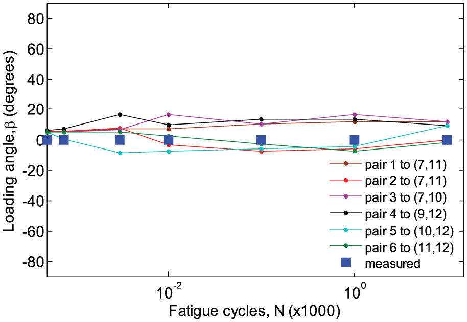
Figures 24 and 25 show the quantification scheme computed values against the measured values for load direction and total crack density, respectively. Estimated loading direction $β$ fluctuates from 16° to −10°. This fluctuation will not affect significantly the stiffness degradation model values. In Figure 25, crack density estimates follow the same trend as the experimental crack density and the values are within the measurement errors.

Figure 24.

Experimental and computed load direction for different path pairs.

Figure 25.

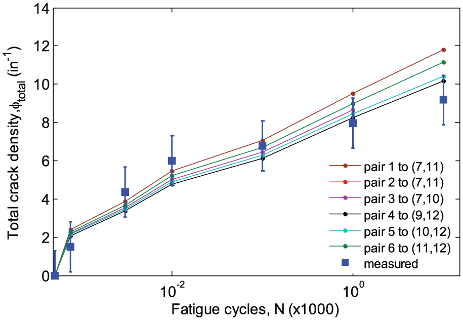
Experimental and estimated crack density for different path pairs.

These results show that the crack quantification scheme and DI model developed produce reasonable estimates for loading direction and crack density. Note that both loading direction and crack density estimates fluctuate as the path pairs used for the nonlinear solution change. This fluctuation is small and for this study deemed reasonable, but it suggests that there is sensitivity to the choice of off-axis angle for a given path pair.

In a sensor network scheme were there are many diagnostic paths intersecting each other and/or covering different areas, the information per path only represents one estimate for a limited zone. But in order to get an overall laminate distributed cracking density estimate, the information from all these paths can be merged and combined. Once the nonlinear set of equations was solved using a specified diagnostic path pair, the loading direction is known, and the crack quantification model simplifies to

ϕ_{total}^{path} = n^{*} g (θ) {(- \ln (1 - \frac{Δ PS D_{θ}}{m^{*} P (θ)}))}^{\frac{1}{2}}

(21)

Equation 12 computes a matrix crack density estimate for each path given that path’s sensor data. With crack density for each path available, a simple triangulation diagnosis algorithm presented in Larrosa and Chang³⁴ was implemented and tested against experimental results for the [90₂/45/−45]₂s laminate.

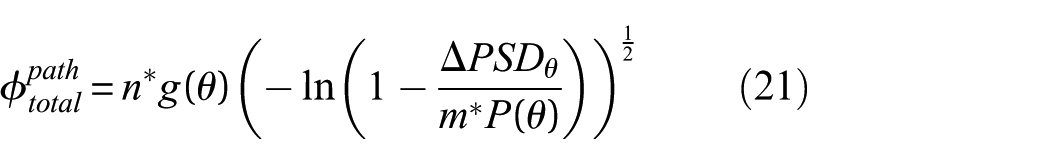
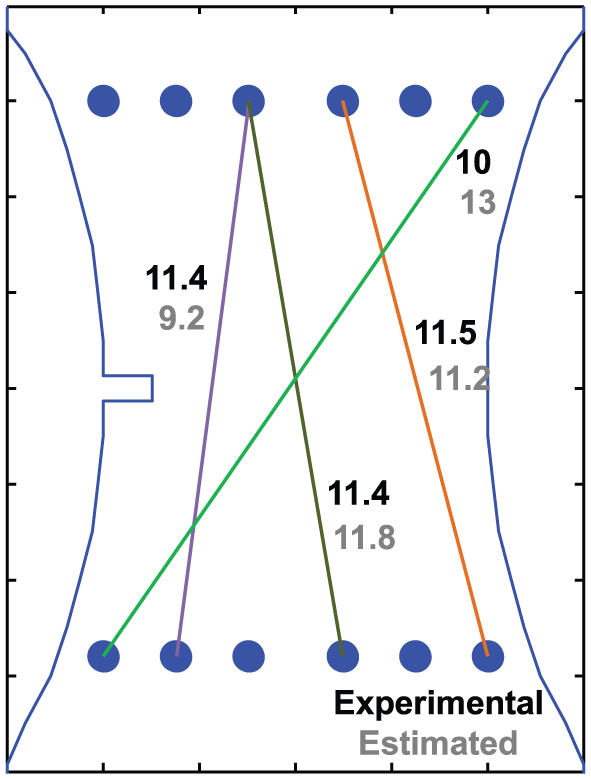
Crack density estimates after 10,000 fatigue cycles for different diagnostic paths compared to the experimental values are shown in Figure 26. Figure 27 shows the resulting crack density diagnosis after taking the path estimates away from the sample’s edges. The same diagnosis algorithm was used for either the SHM estimated or experimental crack density per path values. Similar results were obtained for different cycle intervals. These results suggest that the monitoring method developed outputs reasonably good crack density estimates.

Figure 26.

Crack density (cracks/in) path estimates for [90₂/45/−45]₂s sample after 10,000 cycles.

Figure 27.

Experimental and estimated diagnosis for [90₂/45/−45]₂s sample after 10,000 cycles.

Conclusion

Composite samples instrumented with attached piezoelectric actuators and sensors were subjected to repeated loading to induce transverse matrix cracking and delamination. Through the attached actuators and sensors, ultrasonic wave propagation was captured as crack density increased. Signal changes with crack density were investigated in detail. After detail analysis of the experimental data, it was found that

The signal’s PSD change correlates to crack density and was selected as the DI.

The DI was sensitive to the actuator to sensor orientation, or off-axis angle.

A Rayleigh cumulative distribution function represents the relationship between DI and crack density, where the saturation and scale parameters are dependent on off-axis angle.

Comparing the stiffness degradation model parameters to the DI function parameters as off-axis angle changes, a linear relationship was established. These relationships’ slopes are independent of off-axis angle but dependent on layup stacking sequence. A DI model was proposed and tested against experimental data for [0₂/90₄]s cross-ply laminates. Furthermore, a practical calibration procedure was established in order to find the layup dependent m and n parameters.

With this DI quantification model at hand, a crack density monitoring method was developed and tested on [90₂/45/−45]₂s laminates. The main inputs are layup stacking sequence, material properties and the calibration parameters. The output is total crack density and loading direction. The method requires a minimum of two actuators to sensor paths at different off-axis angles.

The monitoring method estimates were tested against experimentally measured values, and its crack density estimates matched experimental crack density values within established error bounds. Sensitivity to the off-axis angle of these two paths was observed and should be the focus of future studies.

Footnotes

Acknowledgements

The authors would like to acknowledge the National Aeronautics and Space Administration (NASA) for supporting this work under grants ARMD/AvSafe NRA-07-IVHM1-07-0061, NRA-07-IVHM1-07-0064, Space Act Agreement SAA2-402292, and the Air Force Office of Scientific Research (AFOSR) MURI FA9550-09-1-0677. The authors would like to thank Richard W. Ross (NASA LaRC) and Dr Les Lee as the program monitors of the grants, as well as Kai Goebel and Abhinav Saxena (NASA Ames, PCoE) for assistance with experimental planning and support. The authors are also grateful for Acellent Technology’s assistance with the active sensing system.

Declaration of Conflicting Interests

The author(s) declared no potential conflicts of interest with respect to the research, authorship, and/or publication of this article.

Funding

The author(s) received no financial support for the research, authorship, and/or publication of this article.

References

Beaumont

PWR

Dimant

Shercliff

HR.

Failure processes in composite materials: getting physical. J Mater Sci 2006; 41: 6526–6546.

Guided Lamb waves for identification of damage in composite structures: a review. J Sound Vib 2006; 295: 753–780.

Abrate

Matrix cracking in laminated composites: a review. Compos Eng 1991; 1(6): 337–353.

Shahid

Chang

F-K.

Progressive failure analysis of laminated composites subjected to in-plane and shear loads. PhD Dissertation, Department of Aeronautics and Astronautics, Stanford University, Stanford, CA, 1993.

Harris

Allen

Nottorf

. Modelling stiffness loss in quasi-isotropic laminates due to microstructural damage. J Eng Mater: T ASME 1988; 110: 128–133.

Nairn

The initiation and growth of delaminations induced by matrix microcracks in laminated composites. Int J Fracture 1992; 57: 1–24.

Talreja

Damage development in composites: mechanisms and modelling. J Strain Anal Eng 1989; 24(4): 215–222.

Harris

Fatigue in composites. Cambridge: Woodhead Publishing, 2003.

Mueller

Larrosa

Roy

. An integrated diagnostic to prognostic SHM technology for structural health management. In: Proceedings of the 7th international workshop on structural health monitoring, September 2009, vol. 1, pp. 399–409. DEStech Publications, Inc.

10.

Djordjevic

. Nondestructive test technology for composites. In: Proceedings of the 10th international conference of the Slovenian society for non-destructive testing, Ljubljana, 1–3 September 2009.

11.

Liu

Forsyth

Komorowski

. Survey: state of the art in NDE data fusion techniques. IEEE T Instrum Meas 2007; 56(6): 2435–2451.

12.

Farrar

Worden

An introduction to structural health monitoring. Philos T Roy Soc A 2007; 365: 303–315.

13.

Ihn

J-B

Chang

F-K

. Detection and monitoring of hidden fatigue crack growth using a built-in piezoelectric sensor/actuator network: I. Diagnostics. Smart Mater Struct 2004; 13: 609–620.

14.

Lin

Qing

Kumar

. SMART layer and SMART suitcase for structural health monitoring applications. In: Proceedings of SPIE 4332, smart structures and materials 2001: industrial and commercial applications of smart structures technologies, Newport Beach, CA, 14 June 2001, vol. 4332, pp. 98–106. Bellingham, WA: SPIE.

15.

Pierce

Culshaw

Manson

. The application of ultrasonic Lamb wave techniques to the evaluation of advanced composite structures. In: Proceedings of SPIE 3986, smart structures and materials 2000: sensory phenomena and measurement instrumentation for smart structures and materials, Newport Beach, CA, 12 June 2000, vol. 3986, pp. 93–103. Bellingham, WA: SPIE.

16.

Seala

Smith

Prosser

WH.

Lamb wave assessment of fatigue and thermal damage in composites. J Acoust Soc Am 1998; 103(3): 2416–2424.

17.

Worden

Rayleigh and Lamb waves—basic principles. Strain 2001; 37(4): 167–172.

18.

Ihn

J-B

Chang

F-K

. Detection and monitoring of hidden fatigue crack growth using a built-in piezoelectric sensor/actuator network: II. Validation using riveted joints and repair patches. Smart Mater Struct 2004; 13: 621–630.

19.

Ihn

J-B

Chang

F-K.

Pitch-catch active sensing methods in structural health monitoring for aircraft structures. Struct Health Monit 2008; 7: 5–19.

20.

Geetha

Rathod

Chakraborty

. Rapid localization and ultrasonic imaging of multiple damages in structural panel with piezoelectric sensor-actuator network. In: Proceedings of the 8th international workshop on structural health monitoring, September 2011, vol. 2, pp. 249–256. DEStech Publications, Inc.

21.

Time-domain localized structural damage identification with incomplete excitation measurements. In: Proceedings of the 8th international workshop on structural health monitoring, September 2011, vol. 2, pp. 175–182. DEStech Publications, Inc.

22.

Peng

Sun

. Wave propagation analysis in composite laminates containing a delamination using a three-dimensional spectral element method. Math Probl Eng 2012; 2012: 659849 (19 pp.).

23.

Moll

Schulte

Hartmann

. Multi-site damage localization in anisotropic plate-like structures using an active guided wave structural health monitoring system. Smart Mater Struct 2010; 19(4): 045022.

24.

Mujica

Ruiz

Pozo

. Damage detection index based on statistical inference and PCA. In: Proceedings of the 8th international workshop on structural health monitoring, September 2011, vol. 2, pp. 159–174. DEStech Publications, Inc.

25.

C-T

Veidt

Scattering of the fundamental anti-symmetric Lamb wave at delaminations in composite laminates. J Acoust Soc Am 2011; 129(3): 1288–1296.

26.

Toyama

Yashiro

Takatsubo

. Stiffness evaluation and damage identification in composite beam under tension using Lamb waves. Acta Mater 2005; 53: 4389–4397.

27.

Gibson

RF.

Principles of composite material mechanics. Boca Raton, FL: CRC Press, 2011.

28.

Larrosa

Monitoring matrix cracking in composite laminate using built-in piezoelectric sensors. Doctoral Dissertation, Stanford University, Stanford, CA, 2013.

29.

Saxena

Goebel

Larrosa

, et al. Accelerated aging experiments for prognostics of damage growth in composite materials. In: Proceedings of the 8th international workshop on structural health monitoring, September 2011, vol. 2, pp. 1283–1291. DEStech Publications, Inc.

30.

Larrosa

Lonkar

Shankar

. Damage classification in composite laminates; matrix micro-cracking and delamination. In: Proceedings of the 8th international workshop on structural health monitoring, September 2011, vol. 2, pp. 191–199. DEStech Publications, Inc.

31.

Larrosa

Janapati

Roy

. In-situ damage assessment of composite laminates via active sensor networks. In: Proceedings of the 2011 aircraft airworthiness and sustainment conference, San Diego, CA, 18–21 April 2011.

32.

ASTM D3039/D3039M-08. Standard test method for tensile properties of polymer matrix composite materials.

33.

ASTM D3479/D3479M-96:2007. Standard test method for tension-tension fatigue of polymer matrix composite materials.

34.

Larrosa

Chang

F-K

. Real time in-situ damage classification, quantification and diagnosis for composite structures. In: Proceedings of the 19th international congress on sound and vibration, Vilnius, 8–12 July 2012.