Statistical damage localization with stochastic load vectors using multiple mode sets

Abstract

The stochastic dynamic damage locating vector method is an output-only damage localization method based on both a finite element model of the structure and modal parameters estimated from output-only measurements in the damage and reference states of the system. A vector is obtained in the null space of the changes in the transfer matrix from both states and then applied as a load vector to the model. The damage location is related to this stress where it is close to zero. In previous works, an important theoretical limitation was that the number of modes used in the computation related to the transfer function could not be higher than the number of sensors located on the structure. It would be nonetheless desirable not to discard information from the identification procedure. In this article, the stochastic dynamic damage locating vector method has been extended with a joint statistical approach for multiple mode sets, overcoming this restriction on the number of modes. Another problem is that the performance of the method can change considerably depending on the Laplace variable where the transfer function is evaluated. Particular attention is given to this choice and how to optimize it. The new approach is validated in numerical simulations and on experimental data, where the outcomes for multiple mode sets are compared with only using a single mode set. From these results, it can be seen that the success rate of finding the correct damage localization is increased when using multiple mode sets instead of a single mode set.

Keywords

Damage localization load vectors covariance analysis hypothesis testing modal truncation

Introduction

Vibration-based structural health monitoring (SHM) techniques have been actively developed in the last decades,^1–3 for example, for the monitoring of bridges, buildings, or offshore structures. Physical changes in the structure due to damage induce changes in the modal characteristics of the structure, which can be monitored through output-only vibration measurements.

Monitoring-based structural diagnosis is usually divided into five subtasks of increasing difficulty:⁴ damage detection (level 1), damage localization (level 2), identification of damage type (level 3), quantification of the damage extent (level 4), and prediction of the remaining service life (level 5). When performing these tasks in a cascade fashion, the full structural diagnosis problem is amenable to a solution. Methods for damage detection have reached some maturity so far, for example, with data-driven algorithms adapted from pattern classification and statistical process control.^1,5–9

While damage detection can operate purely data-driven, by comparing a current dataset to a reference, damage localization requires some link between the data and the physical properties of the structure, which is often given by a finite element (FE) model of the structure or by directly assuming specific structural types like beams, plates, or rotating machinery in their derivation. Data-driven damage localization methods^2,3 are usually designed for particular structural types, often in combination with dense sensor grids, and are not easily generalizable to arbitrary structural types. Model-based methods update the parameters of an FE model of the healthy structure based on measurements from the damaged system, and damage is located in the regions of the model where parameters are modified.^10,11 While this approach is applicable to arbitrary structural types, it is often too poorly conditioned to be successful in practice due to the huge FE parameter dimension in comparison with relatively few modal parameters that can be extracted from data, and often user interaction is required by an experienced engineer in the updating process.

Alternative damage localization methods with a theoretical background combine properties of the data-driven and model-based approaches. They are based on data-driven features from measurements of the reference and damaged states, which are confronted to an FE model of the investigated structure to define damage indicators for the elements of the FE model, without updating its parameters.¹² For example, localization can be performed by statistical tests on a parameterized residual vector that is computed from measurements^13,14 or by interrogating changes in the flexibility of a structure^15,16 and extracting localization information based on the FE model.

Belonging to the latter category, the stochastic dynamic damage locating vector (SDDLV) approach¹⁶ is a vibration-based damage localization technique using both FE information and modal parameters estimated from output data. Damage is assumed to be related to stiffness loss, which is coherent with common damage models.^17,18 From the modal estimates in both reference and damaged states, a vector in the null space of the difference between the respective transfer matrices is obtained at the sensor positions for some Laplace variable $s$ in the complex plane. It has been shown that when applying this load vector to the FE model of the healthy structure, the resulting stress field is zero at the damaged element. Since the estimates of the modal parameters are naturally subjected to variance errors,^19–24 the resulting stress estimate is not exactly zero at the damaged element, but only close to zero. Based on that uncertainty information, a statistical extension of the SDDLV method was developed by Döhler and colleagues^25,26 for deciding whether an element is damaged.

In previous works on the SDDLV,^16,25–27 the number of sensors needed to be at least as high as the number of identified modes. This is a restriction when more modes are identified from the measurements than the available number of sensors, and not all the available information could be taken into account. At the same time, it is desirable to perform damage localization with a low number of sensors. In this article, the SDDLV method is developed with a joint statistical evaluation using multiple mode sets, overcoming the limitation on the number of sensors and taking into account all identified modal information. It is demonstrated that the computation of stress for multiple mode sets increases the information content about the damaged or non-damaged elements of the structure with respect to a limited number of modes. Finally, all stress values corresponding to each element are tested for damage in a statistical hypothesis test where the computed stresses are evaluated with their joint covariance.

Assessing the performance of the method is a requirement for showing the benefits of this approach. A proper criterion for the evaluation of the success rate is proposed based on Monte-Carlo simulations. The performance of the SDDLV approach is strongly dependent on the choice of the Laplace variable $s$ where the transfer function is evaluated due to the different influence of modal truncation errors. Accommodating multiple $s$ -values has been treated in Marin et al.²⁶. Still, the choice of the Laplace variable is a complicated part of the procedure, even if past guidelines suggest choosing this variable around the identified modes in the complex plane to reduce modal truncation errors. This motivates the performance analysis of the method in Monte-Carlo simulations for many $s$ -variables in the complex plane in this article, where the success rate of correct damage localization is evaluated in dependence of the $s$ -values. The performance of the proposed approach is evaluated under the requirement that the particular choice of $s$ should not be critical. Indeed, the simulation results show that the effect of $s$ -values with poor performance is mitigated when treating all available modes with the statistical multiple mode set strategy of this article. This leads to significant improvement in the localization success rate with the proposed method and less dependence on the particular choice of the $s$ -values.

This article is organized as follows. First, the SDDLV method is presented and the removal of the limiting restriction on the number of modes is discussed using multiple mode sets. Then, the statistical damage localization approach is derived using these multiple mode sets. Finally, the new approach is applied on numerical simulations and experimental data to evaluate the performance of the approach, and conclusions of the work are given.

Damage localization approach (SDDLV)

The SDDLV approach is an output-only damage localization method based on interrogating changes $δ G (s)$ in the transfer matrix $G (s)$ of a system in both reference and damaged states,¹⁶ where $s$ is a Laplace variable in the complex plane. A vector is obtained in the null space of $δ G (s)$ from system identification results using output-only measurements corresponding to both states. Then, this load vector is applied to the FE model of the structure for the computation of a stress field over the structure. The damage is located where the computed stress is zero or close to zero in practice.^15,16 In this section, the deterministic computation of the stress field for damage localization is summarized.

Modeling

We assume that the behavior of a mechanical structure can be described by a linear time-invariant (LTI) dynamic system

M \overset{\cdot\cdot}{X} (t) + C \overset{\cdot}{X} (t) + K X (t) = f (t)

(1)

where $M$ , $C$ , and $K \in R^{d \times d}$ are the mass, damping, and stiffness matrices, respectively; $t$ indicates continuous time; and $X \in R^{d}$ denotes the displacements at the $d$ degrees of freedom (DOF) of the structure. The external force $f (t)$ is not measurable and modeled as white noise.

Let the dynamic system (1) be observed at $r$ coordinates, where often $r << d$ in practice. Since $f (t)$ is unmeasured, it can be substituted with a fictive force $e (t) \in R^{r}$ acting only in the measured coordinates and that regenerates the measured output. Furthermore, defining $x = [X^{T} {\overset{\cdot}{X}}^{T}]^{T}$ , this leads to the corresponding continuous-time state-space model

{\begin{matrix} \overset{\cdot}{x} (t) = A_{c} x (t) + B_{c} e (t) \\ y (t) = C_{c} x (t) + D_{c} e (t) \end{matrix}

(2)

with state vector $x \in R^{n}$ , output vector $y \in R^{r}$ , the state transition matrix $A_{c} \in R^{n \times n}$ , and output matrix $C_{c} \in R^{r \times n}$ , where $n = 2 d$ is the system order and $r$ is the number of outputs. Since the input of the system is replaced by the fictive force $e \in R^{r}$ , the input influence matrix and direct transmission matrix are of size $B_{c} \in R^{n \times r}$ and $D_{c} \in R^{r \times r}$ , respectively. However, only the system matrices $A_{c}$ and $C_{c}$ are relevant from output-only system identification, and the non-identified matrices $B_{c}$ and $D_{c}$ will only be needed in the derivation of estimates related to the transfer matrix. From stochastic subspace identification (SSI),^28–30 modal parameter estimates and subsequently the estimates ${\hat{A}}_{c}$ and ${\hat{C}}_{c}$ can be obtained from output-only measurements, details are given in Appendix 1.

Note that environmental variability, for example, due to temperature changes, may affect the structural properties or boundary conditions and thus the modal parameter estimates.³¹ These effects are not taken into account in the presented models. Since the considered damage localization approach operates on the modal parameter estimates, and environmental variability can be removed from these estimates in a preprocessing step with diverse methods,^5,32 we do not consider this problem further in this article.

Computation of damage indicator

The damage indicator is based on the transfer matrix difference $δ G (s)$ between reference and damaged states. However, the transfer matrix

G (s) = C_{c} (sI - A_{c})^{- 1} B_{c} \in C^{r \times r}

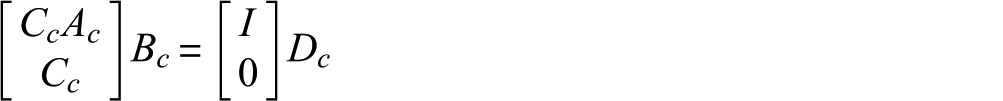
itself cannot be estimated from output-only measurements since matrices $B_{c}$ and $D_{c}$ cannot be estimated. Matrix $B_{c}$ can be replaced using the relationships^16,27

\begin{matrix} C_{c} B_{c} = 0 \\ C_{c} A_{c} B_{c} = D_{c} \end{matrix}

and formulating the least-squares problem

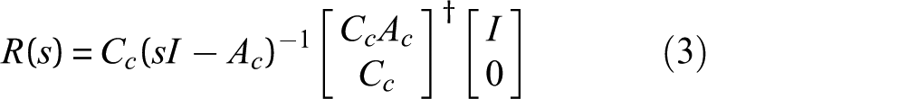
[\begin{matrix} C_{c} A_{c} \\ C_{c} \end{matrix}] B_{c} = [\begin{matrix} I \\ 0 \end{matrix}] D_{c}

which has a solution for $B_{c}$ under the condition that the system order satisfies $n \leq 2 r$ , that is, the number $m$ of identified modes satisfies $m \leq r$ . Then^16,27

G (s) = R (s) D_{c}

where

R (s) = C_{c} (sI - A_{c})^{- 1} {[\begin{matrix} C_{c} A_{c} \\ C_{c} \end{matrix}]}^{†} [\begin{matrix} I \\ 0 \end{matrix}]

(3)

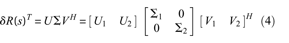
In equation (3), $I$ is the identity matrix of size $r \times r$ , 0 is the zero matrix of size $r \times r$ , $and †$ denotes the Moore–Penrose pseudoinverse. The difference between the transfer matrices in both damaged (variables with tilde) and healthy states is $δ G (s) = \tilde{G} (s) - G (s)$ . Assume that damage is due to changes in stiffness and mass is constant. Then, $D_{c} = {\tilde{D}}_{c}$ , and the matrices $δ G (s)$ and $δ R (s)^{T} = \tilde{R} (s)^{T} - R (s)^{T}$ have the same null space.¹⁶ The desired load vector $v (s)$ is obtained from the null space of the $δ R (s)^{T}$ from singular value decomposition (SVD)

δ R (s)^{T} = U Σ V^{H} = [\begin{matrix} U_{1} & U_{2} \end{matrix}] [\begin{matrix} Σ_{1} & 0 \\ 0 & Σ_{2} \end{matrix}] {[\begin{matrix} V_{1} & V_{2} \end{matrix}]}^{H}

(4)

where $U, Σ, V \in C^{r \times r}$ , $Σ_{2} \approx 0$ , and superscript H indicates the conjugate transpose. Let $n_{im}$ be the dimension of the image $U_{1}$ and $(r - n_{im})$ be the dimension of the null space $V_{2}$ , where $n_{im}$ depends on the kind and number of damaged elements.¹⁵ The load vector $v (s)$ is chosen from the null space $V_{2}$ , for example, as the last column of $V_{2}$ . Note that only output data are necessary for its computation. To compute the stress field over the elements of the structure, the load vector $v (s)$ is applied to the FE model of the structure. First, the vector $v (s)$ is expanded to load vector $ν (s)$ at all DOFs of the model, whose entries are those of $v (s)$ at the sensor coordinates and zero elsewhere. From this vector, the nodal displacements $y (s) = (M s^{2} + Cs + K)^{- 1} ν (s)$ are computed based on the FE model at all DOFs, from which stress resultants are evaluated for each structural element of the model and stacked into stress vector $S (s)$ . This relation between stress and load is linear and can be expressed by a matrix $L_{model} (s) \in C^{l \times r}$ based on the FE model of the structure,^16,25 satisfying

S (s) = L_{model} (s) v (s)

(5)

The stress vector $S (s)$ indicates potential damage for elements with corresponding entries in $S (s)$ that are close to zero.^15,16 When estimated, these stresses are not exactly zero but small in practice because of modal truncation, model errors, and variance errors from measurements.

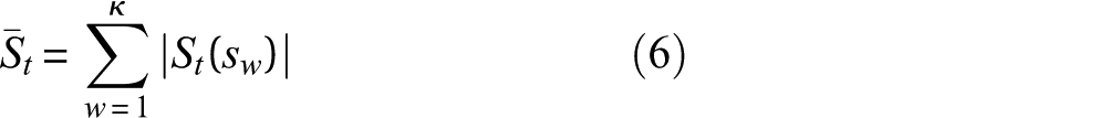
Stress aggregation for robustness

Due to truncation and model errors, it is recommended to compute the load vector $v (s)$ and the resulting stress $S (s)$ for several $s$ -values $s_{w}$ , $w = 1, \dots, κ$ , and to aggregate results. To minimize error, the $s$ -values should be chosen in the vicinity of the identified poles of the system but not too close to them.^16,26 After identification of the system matrices in both states, the computations of (4)–(5) are repeated for each $s_{w}$ to get the respective stress vectors $S (s_{w})$ . For multiple $s$ -values, a deterministic stress aggregation is obtained for each element $t$ as¹⁶

{\bar{S}}_{t} = \sum_{w = 1}^{κ} | S_{t} (s_{w}) |

(6)

In previous works,²⁶ this deterministic aggregation has been replaced by a statistical aggregation, where the intrinsic uncertainty of the stress estimation from finite measurement data is taken into account.

In the following, we address the restriction on the number of modes in the computation of the load vector using multiple mode sets. The resulting stress from each mode set will be statistically aggregated for damage localization.

Multiple mode sets for SDDLV

In practice, there may be more modes available from identification than number of sensors on the structure. It will be meaningful to utilize this information completely from the identification procedure. In the SDDLV,¹⁶ it was not possible to use all modes in this case for the stress computation due to the theoretical restriction $n \leq 2 r$ , where $n = 2 m$ is the system order and $r$ is the number of sensors. Note that $m$ is the number of conjugated complex mode pairs identified from datasets where $m$ has to satisfy the constraint $m \leq r$ .

This constraint is due to the fact that system matrix $B_{c}$ in equation (2) cannot be estimated from output-only measurements for the computation of the transfer matrix. Under this constraint, expression (3) is available, which allows the computation of the load vector in the null space of $δ G (s)$ from output-only measurements.

In order to remove the restriction $m \leq r$ on the number of modes, the computation of stress from different mode sets is investigated in the following, where the current restriction is satisfied for the number of modes in each mode set. This allows considering more than $r$ modes in the analysis. By taking into account more of the identified modes, it is expected that the information content for damage localization should increase. Load vectors and the respective stress are computed for each mode set, using one or several $s$ -values.

Let the identified modes of the system be split into $n_{s}$ mode sets $M_{j}$ , $j = 1, \dots, n_{s}$ , containing $m_{j}$ modes each, where the condition $m_{j} \leq r$ is satisfied for each mode set. Then, the new method of this article takes into account the identified data from all mode sets as follows.

The modal parameters of the structure are identified from SSI using measurement data of the healthy and the damaged states. From the modal parameters corresponding to each mode set $M_{j}$ , the system matrices $A_{c}^{j}$ and $C_{c}^{j}$ are assembled in the healthy and damaged states as detailed in Appendix 1 in equation (22). Then, the computation of the load vector $v^{j} (s)$ is carried out separately for each mode set, that is, the “transfer matrix” resultant $R^{j} (s)$ is computed from both states as in equation (3) and the load vector $v^{j} (s)$ is obtained in the null space of $R^{j} (s)$ from the SVD as in equation (4). The stress vectors $S^{j} (s) = L_{model} (s) v^{j} (s)$ are computed for each mode set and $s$ -value, together with their uncertainty. Finally, damage localization is performed based on a joint statistical evaluation of the computed stresses.

Statistical evaluation for SDDLV using multiple mode sets

For the damage localization algorithm, estimates of the modal parameters are obtained in the damaged and undamaged states using SSI.²⁶ For each mode set, they are the starting point of the computations of the load vectors and associated stresses for damage localization. Their identification is subjected to variance errors because of unknown excitation, measurement noise, and limited data length. The uncertainties in the estimates are penalizing the quality and precision of the damage localization results. For making decisions about damaged elements of the structure, these uncertainties need to be taken into account to decide whether stress of an element is significantly close to zero or not. In previous works,^25,26 the uncertainty of the stress vector $S (s)$ in equation (5) was quantified for a single mode set at one or several $s$ -values. In this section, the uncertainty computation of the stress vector $S^{j} (s)$ is derived for different mode sets $M_{j}$ , $j = 1, \dots, n_{s}$ , for any choice of $s$ , and the joint evaluation of the different stress results is described for each structural element in a statistical test.

The modal parameters are obtained from covariance-driven subspace identification (cov-SSI).^22,29,30 They are estimated from measurement data through the computation of the Hankel matrix $H$ containing the estimated output covariances of the system (see details in Appendix 1). Let $Σ_{H}$ be the covariance of $vec (H)$ , where $vec (\cdot)$ defines the column stacking vectorization operator. This covariance can easily be estimated from the measurement data,^20,22 and the details are given in Appendix 2. Then, the covariance of a vector-valued function $g (H)$ can be approximated by

cov (g (H)) \approx J_{g, H} Σ_{H} J_{g, H}^{T}

(7)

where $J_{g, H} = \partial g (H) / \partial vec (H)$ is the sensitivity of the function $g$ . Since the output covariances and the Hankel matrix are asymptotically Gaussian variables³³ (when number of measurements is large), the statistical delta method³⁴ ensures that expression (7) is asymptotically exact. The required sensitivity can be obtained analytically through a first-order perturbation $Δ g$ of the function $g$ , which yields

Δ g = J_{g, H} vec (Δ H)

(8)

With this strategy, the covariance $Σ_{H}$ of an estimate of Hankel matrix $H$ can be propagated to any function of $H$ , particularly to the modal parameters and to the stress estimate $S (s)$ .

Note that some of the matrices and vectors in the derivation of the damage localization approach are complex-valued variables. To deal with their uncertainties, define an equivalent real-valued notation for any matrix $Q$ as

Q_{Re} =^{def} [\begin{matrix} ℜ (Q) & - ℑ (Q) \\ ℑ (Q) & ℜ (Q) \end{matrix}], Q_{re} =^{def} [\begin{matrix} ℜ (Q) \\ ℑ (Q) \end{matrix}]

$where ℜ (\cdot)$ $and ℑ (\cdot)$ denote the real and imaginary parts, respectively.

For multiple mode sets $M_{j}$ , $j = 1, \dots, n_{s}$ , the sensitivities of the stress estimate $S^{j} (s)$ are derived with respect to estimates $A_{c}^{j}$ , $C_{c}^{j}$ , and subsequently to the Hankel matrix $H$ in both the damaged and healthy states. Then, the covariance of $S^{j} (s)$ can be obtained as in equation (7).

Sensitivity of the system matrices $A_{c}$ and $C_{c}$ from subspace identification

In this section, the covariance of the system matrices $A_{c}^{j}$ and $C_{c}^{j}$ is computed for each mode set $M_{j}$ , starting from the identified eigenvalues $λ_{c, l}^{j}$ and mode shapes $φ_{l}^{j}$ , $l = 1, \dots, m_{j}$ , for each mode set. Based on the SSI approach, their perturbation is linked to the Hankel matrix by

\begin{matrix} Δ λ_{c, l}^{j} = J_{λ_{c, l}^{j}, H} vec (Δ H) \\ Δ φ_{l}^{j} = J_{φ_{l}^{j}, H} vec (Δ H) \end{matrix}

where the sensitivity matrices $J_{λ_{c, l}^{j}, H} \in C^{1 \times h}$ and $J_{φ_{l}^{j}, H} \in C^{r \times h}$ with $h = \dim (vec (H))$ are derived in Reynders et al.²⁰ and Döhler and Mevel.²² The system matrices $A_{c}^{j}$ and $C_{c}^{j}$ are assembled from the eigenvalues and mode shapes for each mode set $M_{j}$ as detailed in Appendix 1. The sensitivities of the vectorized system matrices yield accordingly

vec (Δ A_{c}^{j}) = J_{A_{c}, H}^{j} vec (Δ H)

(9a)

vec (Δ C_{c}^{j}) = J_{C_{c}, H}^{j} vec (Δ H)

(9b)

where the sensitivities $J_{A_{c}, H}^{j}$ and $J_{C_{c}, H}^{j}$ are directly obtained from the eigenvalue and mode shape sensitivities $J_{λ_{c, l}^{j}, H}$ and $J_{φ_{l}^{j}, H}$ as detailed in Marin et al.²⁶

Sensitivity of the stress vector $S^{j} (s)$

Now, the uncertainty of the system matrices is propagated to matrix $R^{j} (s)$ in equation (3) for both healthy and damaged states, then to the load vector in the null space of $δ R^{j} (s)^{T} = {\tilde{R}}^{j} (s)^{T} - R^{j} (s)^{T}$ and finally to the stress vector $S^{j} (s)$ . It holds that

vec (Δ R^{j} (s)^{T})_{re} = J_{R {(s)}^{T}, (A_{c}, C_{c})}^{j} [\begin{matrix} vec (Δ A_{c}^{j}) \\ vec (Δ C_{c}^{j}) \end{matrix}]

(10a)

Δ v^{j} (s)_{re} = J_{v (s), δ R {(s)}^{T}}^{j} (vec (Δ δ R^{j} (s)^{T}))_{re}

(10b)

Δ S^{j} (s)_{re} = (L_{model} (s))_{Re} Δ v^{j} (s)_{re}

(10c)

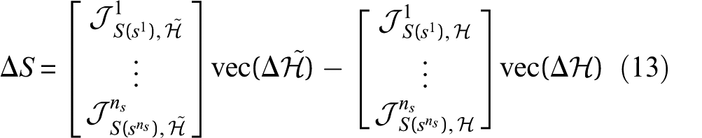
where the respective sensitivity matrices have been derived in detail in Marin et al.²⁶ For a joint evaluation of the stress for multiple mode sets, the uncertainty of the stress needs to be related to a common factor, which is the uncertainty of the Hankel matrix. Combining equations (9) and (10), it holds

Δ S^{j} (s)_{re} = J_{S (s), \tilde{H}}^{j} vec (Δ \tilde{H}) - J_{S (s), H}^{j} vec (Δ H)

(11)

where

\begin{matrix} J_{S (s), H}^{j} = (L_{model} (s))_{Re} J_{v (s), δ R {(s)}^{T}}^{j} J_{R {(s)}^{T}, (A_{c}, C_{c})}^{j} [\begin{matrix} J_{A_{c}, H}^{j} \\ J_{C_{c}, H}^{j} \end{matrix}] \\ J_{S (s), \tilde{H}}^{j} = (L_{model} (s))_{Re} J_{v (s), δ R {(s)}^{T}}^{j} J_{\tilde{R} {(s)}^{T}, ({\tilde{A}}_{c}, {\tilde{C}}_{c})}^{j} [\begin{matrix} J_{{\tilde{A}}_{c}, \tilde{H}}^{j} \\ J_{{\tilde{C}}_{c}, \tilde{H}}^{j} \end{matrix}] \end{matrix}

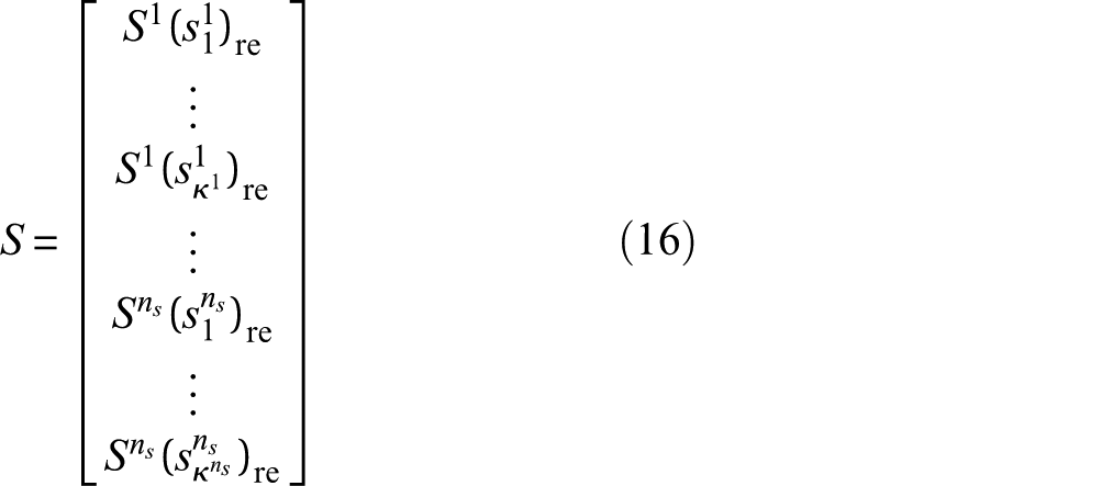
Assume that the stress vector $S^{j} (s)$ is evaluated at a possibly different $s$ -value $s = s^{j}$ for each mode set $M_{j}$ , $j = 1, \dots, n_{s}$ . After stacking the real and imaginary parts of the stress vectors, the total stress vector is derived as

S \overset{def}{=} [\begin{matrix} S^{1} {(s^{1})}_{re} \\ ⋮ \\ S^{n_{s}} {(s^{n_{s}})}_{re} \end{matrix}]

(12)

and its uncertainty follows from (11) as

Δ S = [\begin{matrix} J_{S (s^{1}), \tilde{H}}^{1} \\ ⋮ \\ J_{S (s^{n_{s}}), \tilde{H}}^{n_{s}} \end{matrix}] vec (Δ \tilde{H}) - [\begin{matrix} J_{S (s^{1}), H}^{1} \\ ⋮ \\ J_{S (s^{n_{s}}), H}^{n_{s}} \end{matrix}] vec (Δ H)

(13)

Note that vector $S$ contains the stress information for all mode sets at all elements of the structure.

Joint statistical evaluation of stress

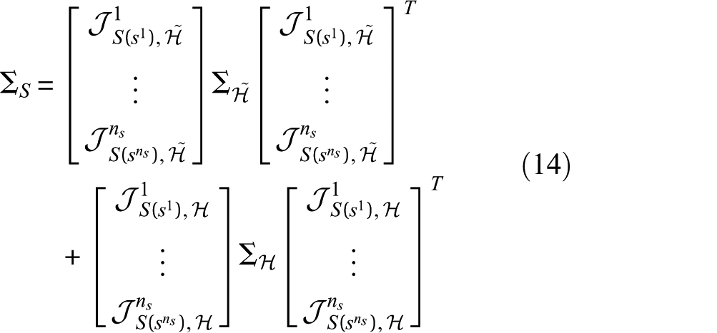
Following from equations (7) and (13), the covariance $Σ_{S} \overset{def}{=} cov (vec (S))$ of the total stress yields

Σ_{S} = [\begin{matrix} J_{S (s^{1}), \tilde{ℋ}}^{1} \\ ⋮ \\ J_{S (s^{n_{s}}), \tilde{ℋ}}^{n_{s}} \end{matrix}] Σ_{\tilde{ℋ}} {[\begin{matrix} J_{S (s^{1}), \tilde{ℋ}}^{1} \\ ⋮ \\ J_{S (s^{n_{s}}), \tilde{ℋ}}^{n_{s}} \end{matrix}]}^{T} + [\begin{matrix} J_{S (s^{1}), ℋ}^{1} \\ ⋮ \\ J_{S (s^{n_{s}}), ℋ}^{n_{s}} \end{matrix}] Σ_{ℋ} {[\begin{matrix} J_{S (s^{1}), ℋ}^{1} \\ ⋮ \\ J_{S (s^{n_{s}}), ℋ}^{n_{s}} \end{matrix}]}^{T}

(14)

since the datasets from reference and damaged states can be regarded as statistically independent. The covariance expression (14) leads to a new statistical approach for damage localization using multiple mode sets based on a statistical test for each element $t$ of the structure. In this approach, all stress components corresponding to a structural element $t$ are collected in a subvector $S_{t}$ of $S$ , containing the information of all mode sets. Accordingly, the respective parts of the covariance matrix $Σ_{S}$ in equation (14) that correspond to element $t$ are collected in $Σ_{t}$ , such that $Σ_{t} = cov (S_{t})$ . Then, vector $S_{t}$ is tested for being zero in a hypothesis test. Since an estimate of the stress vector $S_{t}$ is asymptotically Gaussian distributed, a joint statistical evaluation of the computed stresses is derived in a $χ^{2}$ -test as

χ_{t}^{2} = S_{t}^{T} Σ_{t}^{- 1} S_{t}

(15)

for each structural element $t$ . Since stress over damaged elements is zero in theory, potential damage is located in elements $t$ corresponding to the lowest values of $χ_{t}^{2}$ among all elements.

Joint stress evaluation for different s-values

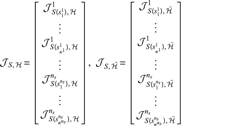
In the previous section, the computation of stress (12) was derived using only one Laplace variable for each mode set while there is a possibility to use several Laplace variables. The computation of stress $S^{j} (s_{w}^{j})$ can be easily generalized for several $s$ -values for each mode set $M_{j}$ , denoted by $s_{w}^{j}$ , where $w = 1, . . ., κ^{j}$ , and $κ^{j}$ is the number of $s$ -values used for mode set $M_{j}$ . After stacking the real and imaginary parts of the stress vectors for multiple $s$ -values and mode sets, the joint stress vector is written analogously as

S = [\begin{matrix} S^{1} {(s_{1}^{1})}_{re} \\ ⋮ \\ S^{1} {(s_{κ^{1}}^{1})}_{re} \\ ⋮ \\ S^{n_{s}} {(s_{1}^{n_{s}})}_{re} \\ ⋮ \\ S^{n_{s}} {(s_{κ^{n_{s}}}^{n_{s}})}_{re} \end{matrix}]

(16)

Then, covariance of the stress (16) with respect to different $s$ -values can be derived together with equation (14) for mode sets $M_{j}$ , $j = 1, \dots, n_{s}$ , as

Σ_{S} = J_{S, \tilde{H}} Σ_{\tilde{H}} J_{S, \tilde{H}}^{T} + J_{S, H} Σ_{H} J_{S, H}^{T}

(17)

where

J_{S, H} = [\begin{matrix} J_{S (s_{1}^{1}), H}^{1} \\ ⋮ \\ J_{S (s_{κ^{1}}^{1}), H}^{1} \\ ⋮ \\ J_{S (s_{1}^{n_{s}}), H}^{n_{s}} \\ ⋮ \\ J_{S (s_{κ^{n_{s}}}^{n_{s}}), H}^{n_{s}} \end{matrix}], J_{S, \tilde{H}} = [\begin{matrix} J_{S (s_{1}^{1}), \tilde{H}}^{1} \\ ⋮ \\ J_{S (s_{κ^{1}}^{1}), \tilde{H}}^{1} \\ ⋮ \\ J_{S (s_{1}^{n_{s}}), \tilde{H}}^{n_{s}} \\ ⋮ \\ J_{S (s_{κ^{n_{s}}}^{n_{s}}), \tilde{H}}^{n_{s}} \end{matrix}]

Analogously to the previous section, the covariance expression (17) leads to a new statistical aggregation scheme for multiple mode sets using several $s$ -values. For each structural element $t$ , the corresponding stress subvector $S_{t}$ of $S$ in equation (16) is selected together with its covariance components $Σ_{t}$ of $Σ$ in equation (17). The stress vector $S_{t}$ is tested for being zero in a statistical hypothesis test as in equation (15) for each structural element $t$ .

Applications

The damage localization method has been applied on numerical simulations and experimental data. A simple mass–spring chain and a more complex three-dimensional (3D) cube beam model have been considered as numerical applications. These numerical applications are idealized test cases for the validation of the new developments of this article, allowing in particular a statistical performance evaluation based on Monte-Carlo simulations. For simplicity, damage is assumed as stiffness loss in elements of a FE model. While no explicit link to a particular origin of such a damage is made, this is coherent with common damage models.^17,18 Finally, the method has been applied to experimental data measured on a beam in a lab experiment.

For each application, the outcome of the damage localization results using multiple mode sets is compared with the ones using only one of the single mode sets separately. To obtain these results from simulated or measured data, the modes of the system are estimated using a stabilization diagram procedure with SSI³⁰ in both reference and damaged states. They are estimated together with their covariance.²² Then, the system matrices and their covariance are assembled from the modes. For each single mode set, the stress vector and its uncertainty are computed. Finally, the estimated stress at the multiple (or single) mode sets and at multiple (or single) $s$ -values is evaluated and statistically aggregated for each structural element with the new method of this article. Comparisons to the deterministic aggregation are based on equation (6). Recall that stress values close to zero indicate potentially damaged elements.

Performance evaluation of damage localization

To analyze the performance of the proposed damage localization method using multiple mode sets, the success rate (or probability) of correct damage localization is evaluated for several sets of simulated measurement data. Each dataset is an independent realization and defines a Monte-Carlo experiment. In order to indicate whether an element is potentially damaged or not, the $χ_{t}^{2}$ value has to be computed for each structural element. For each Monte-Carlo realization, damage localization is seen as successful when the lowest $χ_{t}^{2}$ value among all elements is indeed at the damaged element. The success rate corresponds to the probability of detection or power of the test. Here, it is numerically obtained as the percentage of datasets, among all Monte-Carlo experiments, for which the $χ_{t}^{2}$ value at the damaged element is the smallest $χ_{t}^{2}$ value. The success rate depends on the chosen $s$ -value(s) and serves as the performance indicator of the method when comparing it to localization procedures using only one mode set.

Note that the generation of several datasets allows the evaluation of the success rate, while in reality, usually, only one dataset is available.

In order to evaluate the influence of the $s$ -values on the success rate of damage localization, each dataset in the Monte-Carlo simulations is evaluated for a set of $s$ -values with different real and imaginary parts in order to obtain the success rate in dependence of $s$ . The range of $s$ -values has been chosen in the vicinity of the identified poles to reduce the effects of modal truncation in the transfer matrix estimates.¹⁶ The resulting success rate as a function of $s$ is presented in 3D bar diagrams, where it is plotted on the $z$ -axis in dependence of the real and imaginary parts of $s$ on the $x$ - and $y$ -axis.

Besides the presentation of the success rate of the statistical damage localization using several datasets from Monte-Carlo simulations, the statistical localization approach is compared to the underlying stress computation based on modal parameters from the model (theoretical stress) or from estimates (without statistical evaluation). The theoretical stress evaluation allows to assess the achievable localization accuracy under modal truncation, which is always present in practice. Comparing the localization results from stress estimation and its statistical evaluation allows to evaluate the importance of taking into account the statistical estimation errors in the new method.

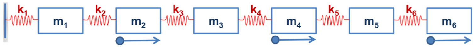
Numerical application 1: mass–spring chain

In a first numerical application, the damage localization method has been applied on a mass–spring chain system with six DOFs as shown in Figure 1. The stiffness parameters are $k_{1} = k_{3} = k_{5} = 4000$ , $k_{2} = k_{4} = k_{6} = 2000$ , and the mass of all elements is 1 in suitable units. Damping is defined such that each mode has a damping ratio of 2%. Damage is simulated by decreasing the stiffness of spring 4 by 10% of its original value. For damaged and undamaged states, the acceleration data length for each set is $N = 50, 000$ . Data were generated from collocated white noise excitation using three sensors at elements 2, 4, and 6 with sampling frequency of 50 Hz, and white measurement noise with 5% magnitude of the outputs was added.

Figure 1.

Mass–spring chain (with modal damping): three sensors.

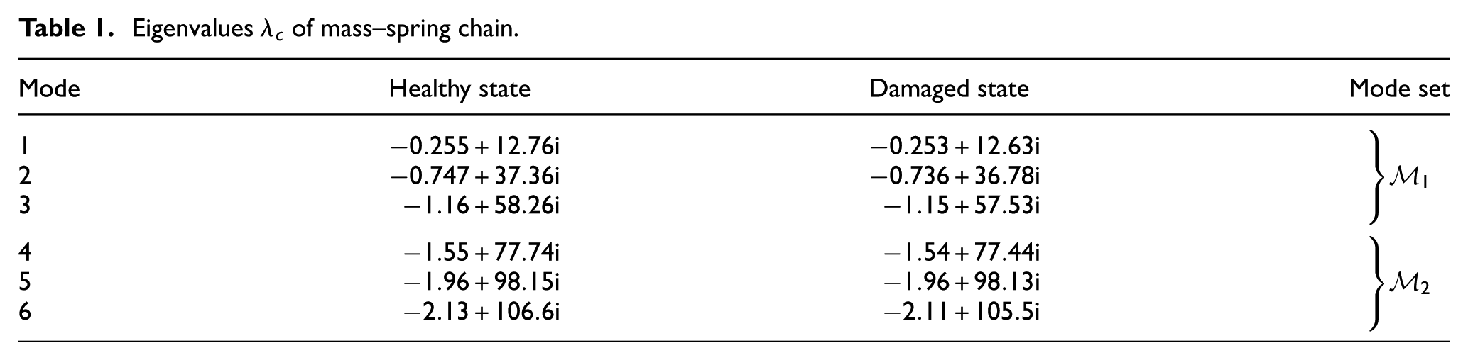
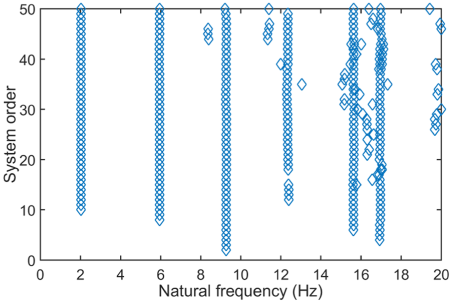
All six modes of the structure (see Table 1) can be identified from the simulated measurements when using SSI. The respective stabilization diagram on a dataset from the healthy state is shown in Figure 2. Using three sensors in this example, only a limited set of three modes could be used for localization in previous works^16,25,26 as the number of modes cannot be bigger than the number of sensors. For the proposed method in this article, all modes can be considered using two mode sets $M_{1}$ and $M_{2}$ of three modes each.

Table 1.

Eigenvalues $λ_{c}$ of mass–spring chain.

Mode	Healthy state	Damaged state	Mode set
1	$- 0.255 + 12.76 i$	$- 0.253 + 12.63 i$	$M_{1}$
2	$- 0.747 + 37.36 i$	$- 0.736 + 36.78 i$
3	$- 1.16 + 58.26 i$	$- 1.15 + 57.53 i$
4	$- 1.55 + 77.74 i$	$- 1.54 + 77.44 i$	$M_{2}$
5	$- 1.96 + 98.15 i$	$- 1.96 + 98.13 i$
6	$- 2.13 + 106.6 i$	$- 2.11 + 105.5 i$

Figure 2.

Stabilization diagram from mass–spring chain simulation in healthy state using SSI.

In the following, localization results at all structural elements are presented for single mode set $M_{1}$ at one $s$ -value, before evaluating the success rate of correct damage localization for single and multiple mode sets at different $s$ -values.

Localization results in all elements for mode set $M_{1}$ at one $s$ -value

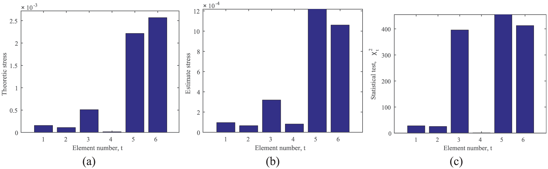
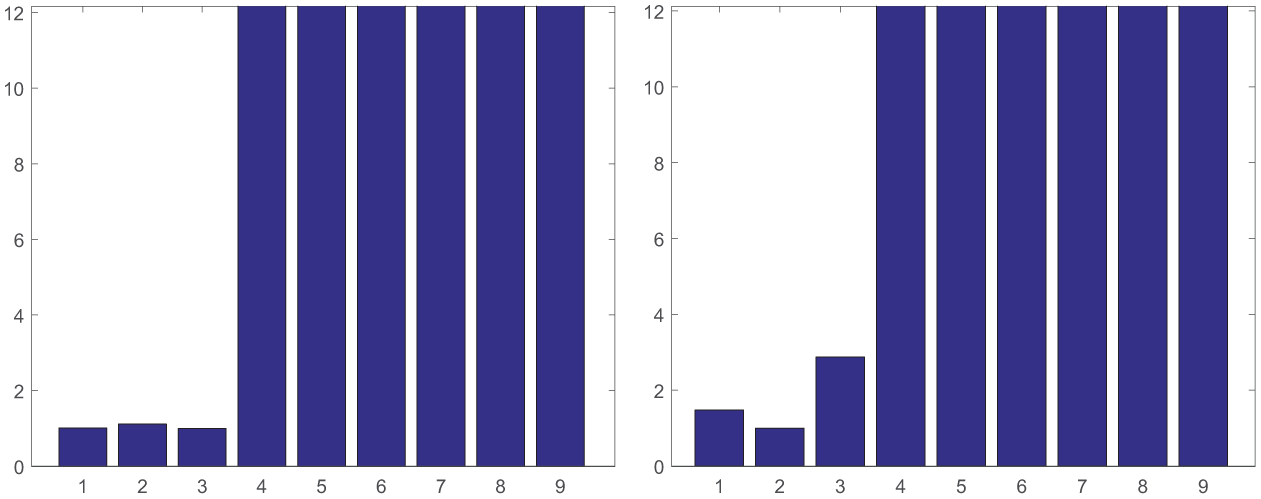
To illustrate the stress computation and its statistical evaluation for damage localization, results for each element of the mass–spring chain are shown in Figure 3 for mode set $M_{1}$ at one $s$ -value. The $s$ -value was chosen in the vicinity of mode set $M_{1}$ as $s = - 2 + 51 i$ . Recall that the damage position is inferred by the stress value closest to zero.

Figure 3.

Localization results at all elements of mass–spring chain using single mode set $M_{1}$ using stress computation and statistical evaluation at $s = - 2 + 51 i$ . Damage is at element 4: (a) stress from exact modal parameters, (b) estimated stress from simulated dataset, and (c) statistical evaluation in $χ_{t}^{2}$ -tests.

In Figure 3(a), the theoretical stress values are computed from the modal parameters corresponding to $M_{1}$ in the healthy and damaged states. The effect of modal truncation leads to stress that is not exactly zero in damaged element 4, but that is close to zero and the smallest compared to the stress at the other elements. When computing the stress from modal parameter estimates from simulated datasets in Figure 3(b), the damage position cannot be correctly indicated anymore, which is probably due to variance errors in the estimation from noisy data. Considering the variance of the modal parameters in the method, the damage position is correctly found since the smallest $χ_{t}^{2}$ value is at element 4 in Figure 3(c).

Success rate of the damage localization using a single mode set

After showing the importance of the statistical evaluation for the estimated stress in the damage localization in the last section, we evaluate the success rates of the statistical damage localization based either on single mode set $M_{1}$ or $M_{2}$ in dependence of the chosen $s$ -value, before going to the joint evaluation of the multiple mode sets in the next section.

For the evaluation of the success rate of correct damage localization at element 4, using either mode set $M_{1}$ or $M_{2}$ , 500 datasets of vibration data were generated for the Monte-Carlo evaluation. Then, the modes of these datasets and their uncertainties were identified using SSI, both in reference and damaged states. Finally, the success rate was determined based on the computation of the $χ_{t}^{2}$ test values in equation (15), using either the modes from $M_{1}$ or $M_{2}$ , for different $s$ -values. The $s$ -values were chosen in the vicinity of the modes (see Table 1) on a global grid with $ℜ (s) \in [- 3, 1]$ and $ℑ (s) \in [0, 130]$ .

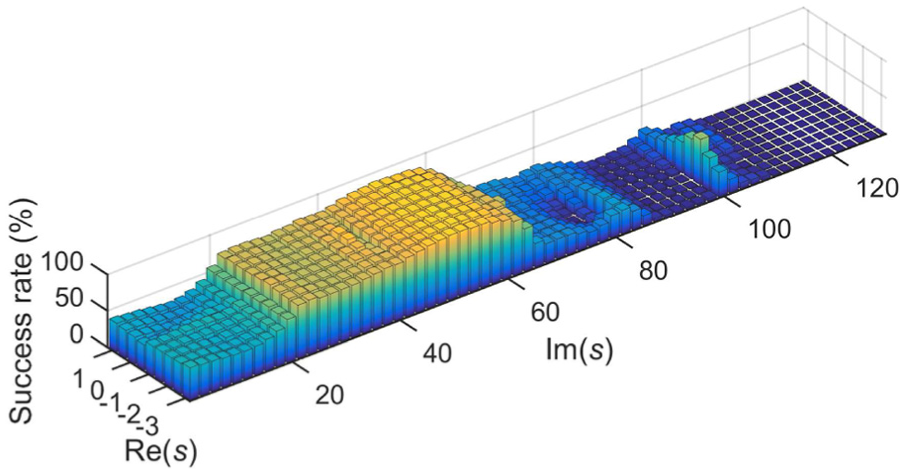
In Figures 4 and 5, the success rates of correct damage localization ( $z$ -axis) are shown in dependence of the real and imaginary parts of the chosen $s$ -values ( $x$ - and $y$ -axis) for mode sets $M_{1}$ and $M_{2}$ , respectively. Indeed, it can be seen that damage localization for both mode sets is satisfactory only for $s$ -values in the vicinity of the modes of the respective mode sets. For mode set $M_{1}$ , corresponding to the first three modes, Figure 4 shows that the success rate is satisfactory only in the interval of the Laplace variables with $ℑ (s) \in [20, 64]$ , where it reaches up to 90%. Beyond this interval, it is close to zero and the damage position cannot be indicated due to the modal truncation error, which is significant outside the interval containing the identified modes (see Table 1).

Figure 4.

Success rate of statistical damage localization using single mode set $M_{1}$ , in dependence of $s$ .

Figure 5.

Success rate of statistical damage localization using single mode set $M_{2}$ , in dependence of $s$ .

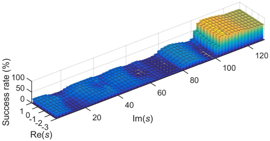
Similarly, for mode set $M_{2}$ corresponding to the last three modes of the structure, it can be seen in Figure 5 that the success rate of damage localization satisfies up to 85% when $ℑ (s)$ belongs to the interval $[102, 128]$ . This area corresponds only to the last two identified modes in $M_{2}$ . While lower performance at $s$ -values around the modes of $M_{1}$ can be expected due to significant modal truncation errors, the success rate at $s$ -values near the fourth mode of the structure is also very low. Hence, choosing the $s$ -value in the vicinity of the identified poles does not necessarily give perfect results.

Success rate of the damage localization using multiple mode sets

In the previous section, the success rate of the damage localization using a single mode set was not successful everywhere in the $s$ -plane mainly because of modal truncation errors. Even considering the $s$ -value in the vicinity of the identified modes, where modal truncation errors should be low, was not sufficient to achieve a reasonable success rate for all choices of $s$ , especially for $M_{2}$ in Figure 5. It cannot be known beforehand where $s$ -values lead to good results in real experiments; however, the only reasonable assumption is to choose them in the vicinity of the identified modes. This motivates the use of the additional information in multiple mode sets instead of using a single mode set alone, expecting better results for the entire $s$ -plane.

For the new statistical approach using multiple mode sets, the $s$ -values are chosen separately for each mode set $M_{1}$ and $M_{2}$ , such that they are in the vicinity of the identified modes of the respective mode set. This means that the $s$ -value $s^{1}$ for mode set $M_{1}$ is chosen with $ℑ (s^{1}) \in [0, 64]$ , and $s^{2}$ for mode set $M_{2}$ with $ℑ (s) \in [66, 128]$ , while the real parts are both in the interval $ℜ (s^{1}), ℜ (s^{2}) \in [- 3, 1]$ .

The impact of the choice of $s$ -values $s^{1}$ and $s^{2}$ when treating the multiple mode sets has been investigated differently for the respective mode sets. The following two cases are now considered:

Case 1: combination of $M_{1}$ and $M_{2}$ with $s$ -values

$s^{1}$ from the entire range in the vicinity of $M_{1}$

$s^{1}$ with $ℑ (s^{2}) = 83$ , where it gave a poor performance using $M_{2}$ only (see Figure 5).

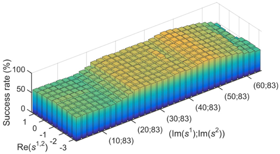
In this case, Figure 6 shows that reasonable success rates are achieved in a large range of $s$ -values compared to the respective single mode sets, even though the performance for the chosen $s^{2}$ was poor in mode set $M_{2}$ . In the interval $ℑ (s^{1}) \in [20, 62]$ , the maximum success rate is achieved, which is slightly lower at 80% than for single mode set $M_{1}$ in Figure 4, but significantly higher than for single set $M_{2}$ at the respective $s$ -value in Figure 5. In the less optimal region with $ℑ (s^{1}) \in [0, 20]$ , the success rate using the multiple mode sets is much higher than in the respective regions using the single mode sets. This shows that combining the information from multiple mode sets strongly mitigates the risk of accidentally choosing $s$ -values with poor performance in the single mode sets. The overall results with the multiple mode sets are as good or better than the ones in both single mode set cases.

Figure 6.

Case 1: success rate of statistical damage localization using multiple mode sets $M_{1}$ and $M_{2}$ , in dependence of $s^{1}$ and $s^{2}$ with $ℑ (s^{1}) \in [0, 64], ℑ (s_{2}) = 83$ .

Case 2: combination of $M_{1}$ and $M_{2}$ with $s$ -values

$s^{1}$ from the entire range in the vicinity of $M_{1}$

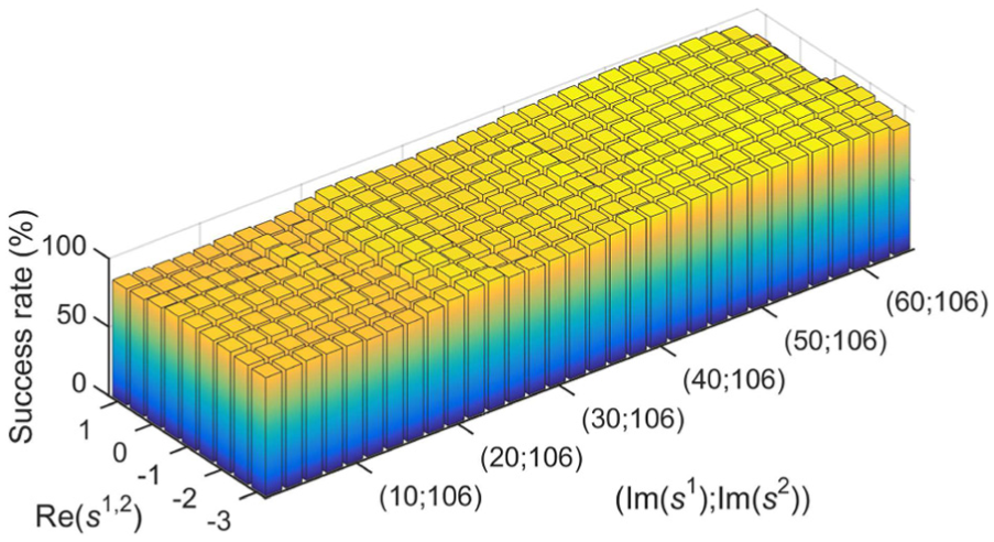
$s^{2}$ with $ℑ (s^{2}) = 106$ , where it gave a good performance using $M_{2}$ only (see Figure 5).

In this case, it can be seen in Figure 7 that the success rate of the damage localization with the new method has significantly improved the situation everywhere in the $s$ -plane, compared to all previous results, with success rates between 85% and 99%.

Figure 7.

Case 2: success rate of statistical damage localization using multiple mode sets $M_{1}$ and $M_{2}$ , in dependence of $s^{1}$ and $s^{2}$ with $ℑ (s^{1}) \in [0, 64], ℑ (s_{2}) = 106$ .

From both cases 1 and 2, it can be concluded that the treatment of all available modes with the statistical multiple mode set strategy of this article improves the damage localization performance, compared to the consideration of using a limited number of modes in a single mode set in the previous approach.^16,25,26 Choices of the respective $s$ -values should be within the vicinity of the respective mode sets. The effect of $s$ -values with poor performance is mitigated, and significant improvement in the localization success rate is made through the statistical combination of results in the approach.

Numerical application 2: 3D cube beam model

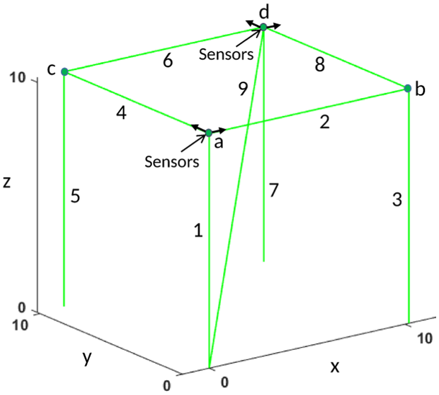
In a second numerical application, the damage localization approach has been demonstrated on a 3D cube beam model as shown in Figure 8, considering a more complex structure than in the previous example. The structure is modeled with nine beam elements of length 10.2 m (except for the diagonal one). The elements are modeled as pipes with internal and external diameters of 1.08 and 1.12 m, respectively. Young’s modulus (E), Poisson’s ratio, and mass density of the beam are 210 GPa, 0.3, and 7800 ${kg . m}^{- 3}$ , respectively. The bottom of the elements 1, 3, 5, and 7 is fixed to the support. The total number of DOFs of the structure is 24. Damage is introduced in element 8 by decreasing Young’s and shear modulus by 50% of its original value. The evaluated stress resultants for each structural element are the real and imaginary parts of the six internal forces $τ_{t} = {\begin{matrix} F_{x} & M_{x} \\ V_{y} & M_{y} \\ V_{z} & M_{z} \end{matrix}}$ where $t$ is the element index, $F_{x}$ is the axial force, $V_{y}$ and $V_{z}$ are the shear forces, $M_{x}$ is the moment of torsion, and $M_{y}$ and $M_{z}$ are the bending moments.

Figure 8.

3D cube model with beam elements (24 DOFs).

For both healthy and damaged states, acceleration datasets of length $N = 200, 000$ are simulated from collocated white noise excitation at four accelerometers in the $x - y$ direction at nodes a and d, at a sampling frequency of 350 Hz. White measurement noise with 5% magnitude of the simulated outputs was added.

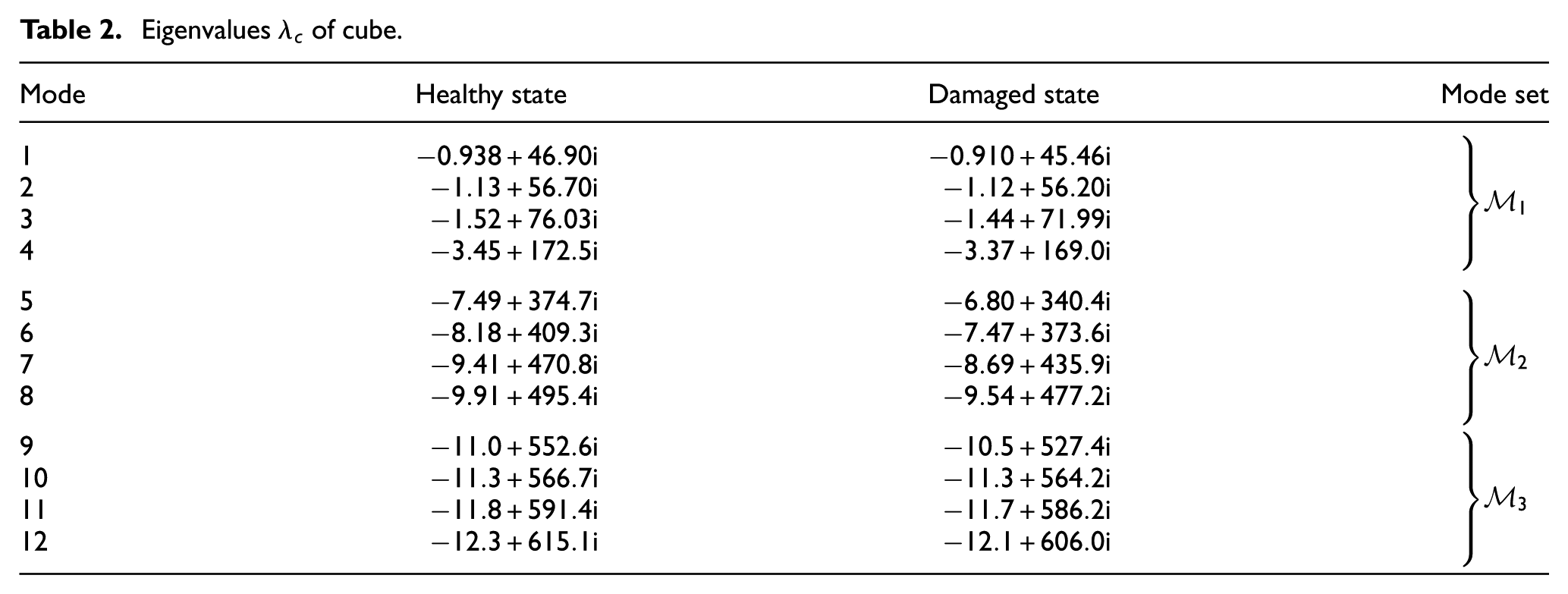
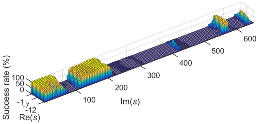
In this example, 13 modes can be well identified from the simulated measurements of the structure with SSI. Using four sensors in this example, only a limited set of four modes could be used for localization in previous works^16,25,26 as the number of modes cannot be bigger than the number of sensors. For localization, we consider the first 12 modes and split into three mode sets $M_{1}$ , $M_{2}$ , and $M_{3}$ of four modes each for the proposed method in this article.

As in the previous example, we analyze the success rate for localization with the mode sets separately in dependence of the chosen $s$ -value, before jointly evaluating it based on all three mode sets with the new method from this article. Monte-Carlo simulations are carried out using 100 simulated datasets in healthy and reference states to determine the success rate, where in each dataset, the modes and their uncertainties are identified using SSI. The entire $s$ -value range in the vicinity of the modes (see Table 2) is $ℜ (s) \in [- 12, - 7] \cup [- 4, - 1]$ and $ℑ (s) \in [0, 650]$ .

Table 2.

Eigenvalues $λ_{c}$ of cube.

Mode	Healthy state	Damaged state	Mode set
1	$- 0.938 + 46.90 i$	$- 0.910 + 45.46 i$	$M_{1}$
2	$- 1.13 + 56.70 i$	$- 1.12 + 56.20 i$
3	$- 1.52 + 76.03 i$	$- 1.44 + 71.99 i$
4	$- 3.45 + 172.5 i$	$- 3.37 + 169.0 i$
5	$- 7.49 + 374.7 i$	$- 6.80 + 340.4 i$	$M_{2}$
6	$- 8.18 + 409.3 i$	$- 7.47 + 373.6 i$
7	$- 9.41 + 470.8 i$	$- 8.69 + 435.9 i$
8	$- 9.91 + 495.4 i$	$- 9.54 + 477.2 i$
9	$- 11.0 + 552.6 i$	$- 10.5 + 527.4 i$	$M_{3}$
10	$- 11.3 + 566.7 i$	$- 11.3 + 564.2 i$
11	$- 11.8 + 591.4 i$	$- 11.7 + 586.2 i$
12	$- 12.3 + 615.1 i$	$- 12.1 + 606.0 i$

In the next section, the success rate of the damage localization results has been computed using the single mode sets separately in Monte-Carlo simulation for 100 datasets. Then, the success rate of the damage localization is illustrated with the new proposed method for the joint statistical evaluation of the multiple mode sets.

Success rate of the damage localization using a single mode set

We evaluate the success rates of the statistical damage localization based either on single mode set $M_{1}$ , $M_{2}$ , or $M_{3}$ in dependence of the chosen $s$ -value, before going to the joint evaluation of the multiple mode sets in the next section.

The $s$ -values were chosen within the global range described above to see the influence of the different $s$ -values also beyond the range of each individual mode set. In Figures 9 to 11, the success rates of correct damage localization ( $z$ -axis) are shown in dependence of the real and imaginary parts of the chosen $s$ -values ( $x$ - and $y$ -axis) for mode sets $M_{1}$ , $M_{2}$ , and $M_{3}$ , respectively. Indeed, it can be seen that damage localization for both mode sets is satisfactory only for $s$ -values in the vicinity of the modes of the respective mode sets.

Figure 9.

Success rate of statistical damage localization using single mode set $M_{1}$ , in dependence of $s$ .

Figure 10.

Success rate of statistical damage localization using single mode set $M_{2}$ , in dependence of $s$ .

Figure 11.

Success rate of statistical damage localization using single mode set $M_{3}$ , in dependence of $s$ .

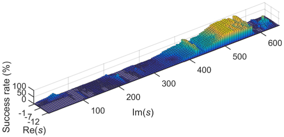
For mode set $M_{1}$ , corresponding to the first four modes in the region $ℑ (s) \in [0, 175]$ , Figure 9 shows that the success rate is satisfactory only in the interval of the Laplace variables with $ℑ (s) \in [0, 81] \cup [120, 201]$ , where it reaches up to 100%. Beyond this interval, it is close to zero and the damage position cannot be indicated due to the modal truncation error, which is significant outside the interval containing the identified modes (see Table 1). However, there is also a region within the vicinity of the modes of $M_{1}$ , where the success rate is close to zero.

The four modes in mode set $M_{2}$ are within the region $ℑ (s) \in [300, 475]$ , and it can be seen in Figure 10 that the success rate of damage localization satisfies the interval $ℑ (s) \in [300, 445]$ , covering nearly the entire region. Possibly, the success rate in the last part of the region is low due to proximity of mode set $M_{3}$ and the resulting truncation errors.

Finally, the success rate for mode set $M_{3}$ is shown in Figure 11, where the modes are in the interval $ℑ (s) \in [450, 625]$ . The success rate is good for $ℑ (s) \in [500, 580]$ , covering only a part of the region corresponding to $M_{3}$ .

Similarly, as in the previous example, this shows that choosing the $s$ -value in the vicinity of the identified poles does not necessarily give perfect results. This motivates the combination of results of different mode sets for more robustness and less dependence on the particular choice of $s$ .

Success rate of the damage localization using multiple mode sets

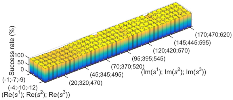
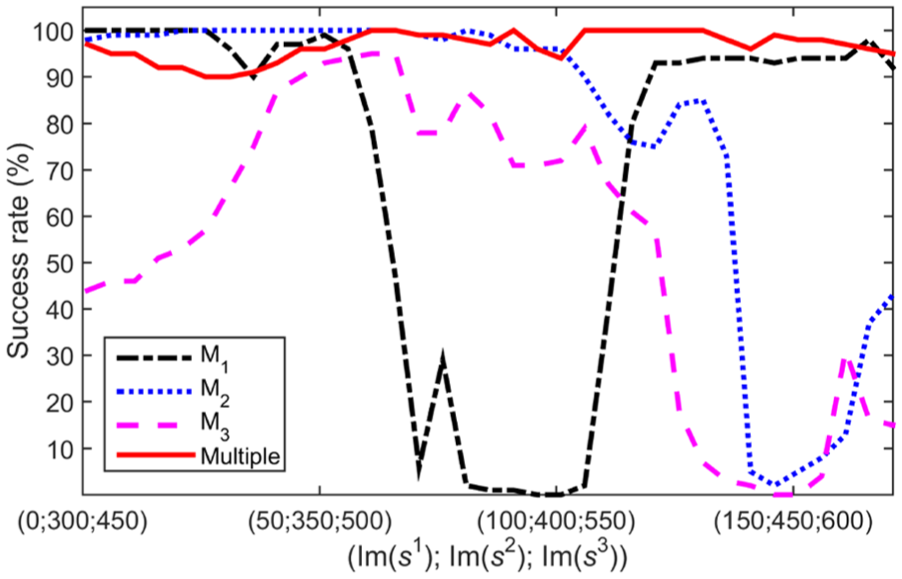
For the new statistical approach using multiple mode sets, the $s$ -values are chosen separately for each mode set $M_{1}$ , $M_{2}$ , and $M_{3}$ , such that they are in the vicinity of the identified modes of the respective mode set. Therefore, the range of the respective $s$ -values $s^{1}$ , $s^{2}$ , and $s^{3}$ is chosen with $ℜ (s^{1}) \in [- 4, - 1]$ , $ℑ (s^{1}) \in [0, 175]$ , $ℜ (s^{2}) \in [- 10, - 7]$ , $ℑ (s^{2}) \in [300, 475]$ , $ℜ (s^{3}) \in [- 12, - 9]$ , $ℑ (s^{3}) \in [450, 625]$ .

The impact of the choice of $s$ -values $s^{1}$ , $s^{2}$ , and $s^{3}$ in the respective mode sets has been investigated for the joint statistical evaluation of the stress, where the evaluation for each triplet $(s^{1}, s^{2}, s^{3})$ is carried out with $s^{1}$ , $s^{2}$ , and $s^{3}$ covering the above range of $s$ -values used in the respective mode sets. In Figure 12, the resulting success rate of the joint evaluation is shown, where it can be seen that the success rate is nearly 100% everywhere in the $s$ -plane. A comparison to the success rates from the single mode sets in the respective range of $s$ -values is made in Figure 13 for fixed real parts $ℜ (s^{1}) = - 3$ , $ℜ (s^{2}) = - 9$ and $ℜ (s^{3}) = - 11$ , where it can be clearly seen that the statistical combination of the results from the single mode set significantly improves the damage localization performance nearly everywhere in the $s$ -plane. In particular, the choice of $s$ -values in the vicinity of the identified modes always yields very good success rates in the joint evaluation of the multiple mode sets, while this was not always the case using the single mode sets separately.

Figure 12.

Success rate of statistical damage localization using multiple mode sets $M_{1}$ , $M_{2}$ , and $M_{3}$ , in dependence of $s^{1}$ , $s^{2}$ , and $s^{3}$ .

Figure 13.

Success rate of statistical damage localization in the single mode sets $M_{1}$ , $M_{2}$ , and $M_{3}$ with $s$ in the vicinity of the respective modes, compared to the success rate using jointly the multiple mode sets.

Experimental application: cantilever beam

Experimental setup and measurements

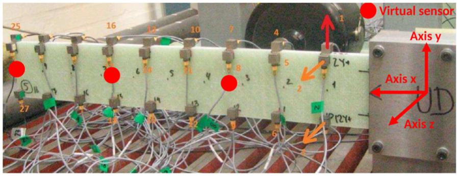
In a lab experiment, damage tests were conducted on a cantilever beam that is made of plastic, as shown in Figure 14. Its dimensions are $0.5 m \times 0.08 m \times 0.01 m$ and it is fixed on one side. Damage was introduced by drilling holes, located at 0.08 m from the fixed end. The beam was excited horizontally by a shaker under white noise excitation and the response was monitored by 18 horizontal and 9 vertical accelerometers. For both the healthy and damaged states, acceleration data of length $N = 295, 936$ with a sampling frequency of $8192 Hz$ were recorded.

Figure 14.

Experimental setup of the beam.

This experimental setup has been used previously as a validation case for the SDDLV method.²⁶ In this previous work, the localization was performed using all the available horizontal sensors. Consequently, using all the signals it was possible to identify natural frequencies and mode shapes in bending and torsion.

The objective of this study is to localize the damage with a minimum number of sensors to highlight the advantage of using the proposed multiple mode set method. Furthermore, it is intended to demonstrate the method based on a very simple FE model of the structure.

Therefore, we consider only three “virtual sensors” located in the center of the structure instead of the full data from the horizontal accelerometers (see Figure 14). The measurements of these three sensors at 0.167, 0.333, and 0.5 m from the fixed end are obtained as the mean of the measured accelerations at the top and bottom of the beam. This means that we are voluntarily excluding the torsional modes. We are able to identify five bending modes in the plane $x - z$ , which will show to be sufficient for a precise damage localization in the following when considering all five modes in two mode sets with the method from this article.

Modal analysis and uncertainties

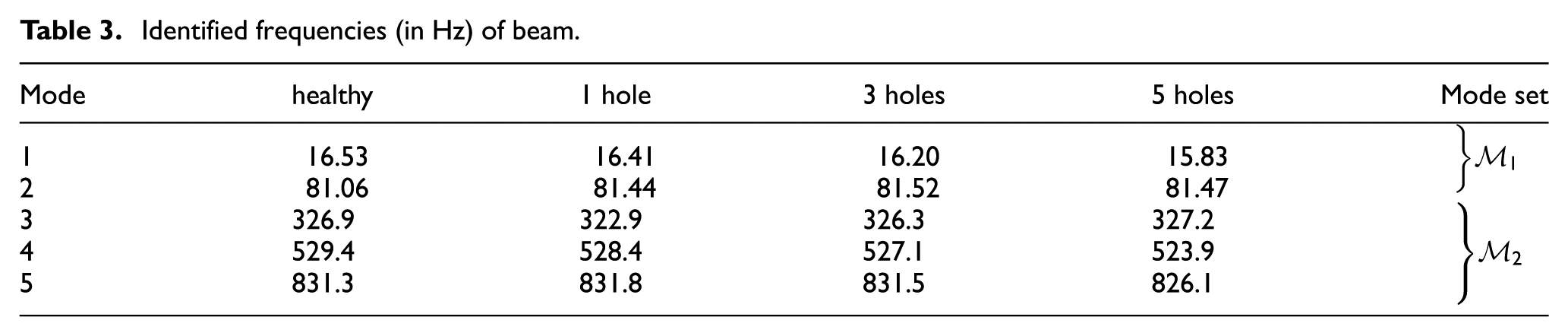
After downsampling and decimation of the data by factor 4, five well-estimated bending modes were obtained in the healthy and the three damaged states from the measurement data using SSI, together with their uncertainties. The identified frequencies are shown in Table 3 for each mode. Since only three sensors are used, the identified modes are split into two mode sets $M_{1}$ and $M_{1}$ containing two and three modes, respectively.

Table 3.

Identified frequencies (in Hz) of beam.

Mode	healthy	1 hole	3 holes	5 holes	Mode set
1	16.53	16.41	16.20	15.83	$M_{1}$
2	81.06	81.44	81.52	81.47	$M_{1}$
3	326.9	322.9	326.3	327.2	$M_{2}$
4	529.4	528.4	527.1	523.9
5	831.3	831.8	831.5	826.1

FE model

The model needs to be as simple as is practicable but it has to correctly represent the behavior of the structure. In this particular example, a simple 2D beam model gives the correct mode shapes for the bending modes in the plane $x - z$ , so it can represent the first five bending modes in the plane $x - z$ of the structure. Considering all the modes, it matches to the modes 1-2-5-6-9 of a 3D model used as reference. Here, the structure is not strictly speaking a beam since the ratio length/width is inferior to 10. This leads to a systematic, but acceptable, model error of about 8% considering the gap between the reference values of the eigenfrequencies obtained with a very fine mesh 3D model and the ones obtained with the analytical beam model.

A trade-off between the model size, that is, the number of DOFs, and the model precision must be considered for the computation of the stress for damage localization. The stress resultants and their uncertainties are computed for each structural element. Using only three sensors, it seems to be reasonable to demand a localization precision within a discretization of nine elements of the beam. Additionally, such a coarse mesh of nine elements is good enough to compute the first five bending modes in the $x - z$ plane. It is finally the model that we have chosen in this study, as depicted in Figure 15.

Figure 15.

Model of the beam with three sensors.

Young’s modulus (E), Poisson’s ratio, and mass density of the beam are chosen as 5 GPa, 0.4, and 1100 ${kg . m}^{- 3}$ , respectively. The computed stress resultants for each structural element are the real and imaginary parts of the three internal forces $τ_{t} = {\begin{matrix} F_{x} & 0 \\ 0 & M_{y} \\ V_{z} & 0 \end{matrix}}$ . The damage is situated at element 2 in this model, being located at 0.08 m from the fixed end.

Localization results at all elements

The performance of the proposed damage localization method using multiple mode sets is compared to the separate single mode set evaluation for the three different damage scenarios.

The localization results are computed at all elements from the experimental datasets in both damaged and healthy states. The computation of the stress and its uncertainties for the statistical evaluation in the $χ_{t}^{2}$ -tests are carried out for two different sets of $s$ -values, each in the vicinity of the respective mode sets. First, one $s$ -value is chosen for each mode set with $s^{1} = - 10 + 90 i$ for mode set $M_{1}$ and $s^{2} = - 10 + 3200 i$ for mode set $M_{2}$ . Second, three $s$ -values are chosen for joint evaluation for each mode set as in equations (16) and (17): $s_{1}^{1} = - 10 + 90 i$ , $s_{2}^{1} = - 10 + 100 i$ , $s_{3}^{1} = - 10 + 200 i$ for $M_{1}$ , and $s_{1}^{2} = - 10 + 2100 i$ , $s_{2}^{2} = - 10 + 3200 i$ , $s_{3}^{2} = - 10 + 3300 i$ for $M_{2}$ . To easily compare the ratios of the stress or associated $χ_{t}^{2}$ -values between the undamaged and damaged elements in the different test cases, the computed values are normalized in the figures such that the smallest value of the nine elements is 1.

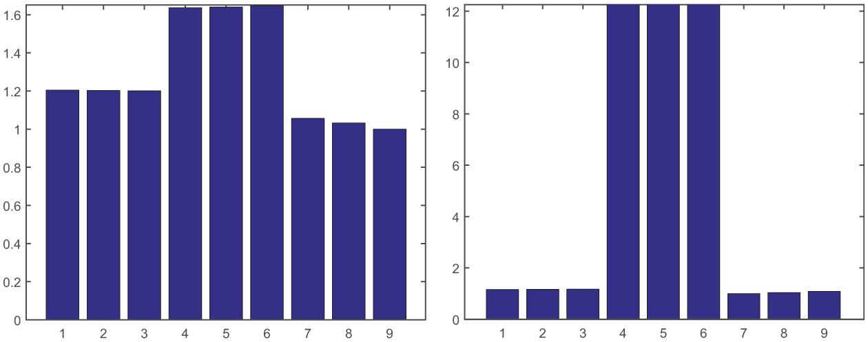
The estimated stress and its statistical evaluation are shown in detail for the first damage case of one hole. In Figures 16 and 17, the results are shown for considering the single mode sets $M_{1}$ and $M_{2}$ . Neither the estimated stress nor its statistical evaluation can correctly indicate the damage at element 2. When using the joint statistical evaluation of both mode sets with the method of this article, the results using one $s$ -value in Figure 18(a) indicate the damaged element within the adjacent elements of the damaged one, being close to correct damage localization. By adding information through two more $s$ -values in the same setting, the damaged element can be correctly indicated in Figure 18(b).

Figure 16.

Localization results for all elements using single mode set $M_{1}$ at $s^{1} = - 10 + 90 i$ . Damage case: one hole: (a) estimated stress and (b) statistical evaluation in $χ_{t}^{2}$ -tests.

Figure 17.

Localization results for all elements using single mode set $M_{2}$ at $s^{2} = - 10 + 3200 i$ . Damage case: one hole: (a) estimated stress and (b) statistical evaluation of $χ_{t}^{2}$ -tests.

Figure 18.

Statistical localization results with new method using both mode sets. Damage case: one hole: (a) one $s$ -value and (b) three $s$ -values.

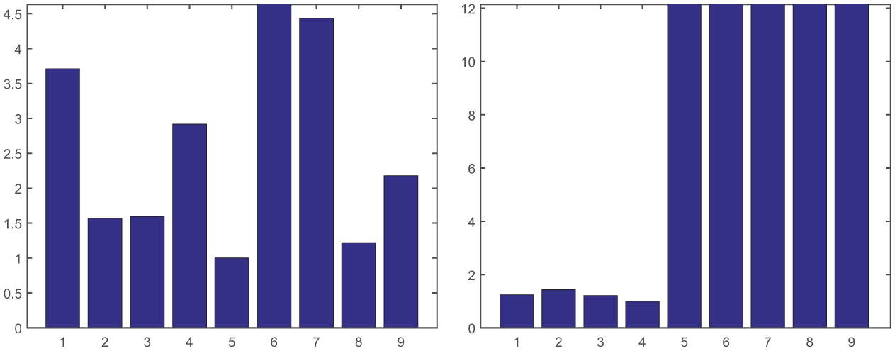
Then, the localization results with the proposed method of this article are presented in Figures 19 and 20 for the further damage severities of three and five holes, showing the joint statistical evaluation of the multiple mode sets using one or three $s$ -values for each mode set. Using one $s$ -value in Figures 19(a) and 20(a), the damage can be localized in the region of the damaged and its adjacent elements, and the $χ_{t}^{2}$ -value for the damaged element 2 is slightly lower than for the neighboring elements. Using three $s$ -values in Figures 19(b) and 20(b), the damage can be more clearly localized in element 2.

Figure 19.

Statistical localization results with new method using both mode sets. Damage case: three holes: (a) one $s$ -value and (b) three $s$ -values.

Figure 20.

Statistical localization results with new method using both mode sets. Damage case: five holes: (a) one $s$ -value and (b) three $s$ -values.

Summarizing the results in this experiment, it can be seen that neither the estimated stress from the SDDLV approach nor its statistical evaluation is sufficient for damage localization in the classical formulation using one mode set, which is probably due to significant modal truncation errors when using only limited modal information. The statistical evaluation with the proposed method takes all the modal information into account and correctly indicates the damage locations in this example, based on measurements from only three sensors and five identified modes, together with a coarse FE model of the structure.

Conclusion

In this article, the damage localization with the SDDLV approach has been extended considering multiple mode sets based on a joint statistical evaluation that takes into account the information from all identified modes of the structure. The stress computation using multiple mode sets increases the information content about the damaged or non-damaged elements of the structure, compared to evaluation from a limited number of modes due to a previous constraint of the approach on the number of modes. With the new approach, this constraint is lifted, which allows damage localization with fewer sensors at the same time. While the stress evaluation for each mode set is naturally subjected to modal truncation errors that depend on the choice of the Laplace variable $s$ , the joint statistical evaluation for several mode sets seems to mitigate these errors. Indeed, the simulation results in the numerical applications show that the effect of $s$ -values with poor performance in single mode set is mitigated when treating all available modes with the statistical multiple mode set strategy of this article. This leads to significant improvement in the localization success rate with the proposed method and less dependence on the particular choice of the $s$ -values, which contributes to the applicability of the method in practice in SHM systems. Finally, the proposed method was able to correctly localize the damage in an experimental application on a damaged cantilever beam with a small number of sensors and using a coarse FE model. Future works should include a detailed analysis of the performance of the localization method under environmental nuisances like temperature changes in combination with methods that remove the environmental variability on modal parameters, in order to further improve the applicability on structures in the field.

Footnotes

Appendix 1

Appendix 2 Acknowledgements

The authors thank Brüel & Kjær for providing the data from the beam experiment.

Declaration of conflicting interests

The author(s) declared no potential conflicts of interest with respect to the research, authorship, and/or publication of this article.

Funding

The first author (M.D.H.B.) was financially supported by the Bretagne region.

References

Farrar

Doebling

Nix

. Vibration-based structural damage identification. Philos T R Soc A 2001; 359(1778): 131–149.

Carden

Fanning

. Vibration-based condition monitoring: a review. Struct Health Monit 2004; 3(4): 355–377.

Fan

Qiao

. Vibration-based damage identification methods: a review and comparative study. Struct Health Monit 2011; 10(1): 83–111.

Farrar

Worden

. An introduction to structural health monitoring. Philos T R Soc A 2007; 365(1851): 303–315.

Deraemaeker

Reynders

De Roeck

. Vibration-based structural health monitoring using output-only measurements under changing environment. Mech Syst Signal Pr 2008; 22(1): 34–56.

Balmès

Basseville

Bourquin

. Merging sensor data from multiple temperature scenarios for vibration-based monitoring of civil structures. Struct Health Monit 2008; 7(2): 129–142.

Döhler

Mevel

Hille

. Subspace-based damage detection under changes in the ambient excitation statistics. Mech Syst Signal Pr 2014; 45(1): 207–224.

Döhler

Hille

Mevel

. Structural health monitoring with statistical methods during progressive damage test of S101 Bridge. Eng Struct 2014; 69: 183–193.

Comanducci

Magalhães

Ubertini

. On vibration-based damage detection by multivariate statistical techniques: application to a long-span arch bridge. Struct Health Monit 2016; 15(5): 505–524.

10.

Brownjohn

JMW

Xia

Hao

. Civil structure condition assessment by FE model updating: methodology and case studies. Finite Elem Anal Des 2001; 37(10): 761–775.

11.

Simoen

De Roeck

Lombaert

. Dealing with uncertainty in model updating for damage assessment: a review. Mech Syst Signal Pr 2015; 56: 123–149.

12.

Limongelli

Chatzi

Döhler

. Toward extraction of vibration-based damage indicators. In: Proceedings of the 8th European workshop on structural health monitoring, Bilbao, 5–8 July 2016.

13.

Balmès

Basseville

Mevel

. Statistical model-based damage localization: a combined subspace-based and substructuring approach. Struct Control Hlth 2008; 15(6): 857–875.

14.

Döhler

Mevel

Zhang

. Fault detection, isolation and quantification from Gaussian residuals with application to structural damage diagnosis. Annu Rev Control 2016; 42: 244–256.

15.

Bernal

. Load vectors for damage localization. J Eng Mech 2002; 128(1): 7–14.

16.

Bernal

. Load vectors for damage location in systems identified from operational loads. J Eng Mech 2010; 136(1): 31–39.

17.

Mazars

. A description of micro-and macroscale damage of concrete structures. Eng Fract Mech 1986; 25(5-6): 729–737.

18.

Zheng

Kessissoglou

. Free vibration analysis of a cracked beam by finite element method. J Sound Vib 2004; 273(3): 457–475.

19.

Pintelon

Guillaume

Schoukens

. Uncertainty calculation in (operational) modal analysis. Mech Syst Signal Pr 2007; 21(6): 2359–2373.

20.

Reynders

Pintelon

De Roeck

. Uncertainty bounds on modal parameters obtained from stochastic subspace identification. Mech Syst Signal Pr 2008; 22(4): 948–969.

21.

Carden

Mita

. Challenges in developing confidence intervals on modal parameters estimated for large civil infrastructure with stochastic subspace identification. Struct Control Hlth 2011; 18(1): 53–78.

22.

Döhler

Mevel

. Efficient multi-order uncertainty computation for stochastic subspace identification. Mech Syst Signal Pr 2013; 38(2): 346–366.

23.

Döhler

Lam

Mevel

. Uncertainty quantification for modal parameters from stochastic subspace identification on multi-setup measurements. Mech Syst Signal Pr 2013; 36(2): 562–581.

24.

Mellinger

Döhler

Mevel

. Variance estimation of modal parameters from output-only and input/output subspace-based system identification. J Sound Vib 2016; 379: 1–27.

25.

Döhler

Marin

Bernal

. Statistical decision making for damage localization with stochastic load vectors. Mech Syst Signal Pr 2013; 39(1–2): 426–440.

26.

Marin

Döhler

Bernal

. Robust statistical damage localization with stochastic load vectors. Struct Control Hlth 2015; 22(3): 557–573.

27.

Bernal

. Flexibility-based damage localization from stochastic realization results. J Eng Mech 2006; 132(6): 651–658.

28.

Van Overschee

De Moor

. Subspace identification for linear systems: theory, implementation, applications. Dordrecht: Kluwer Academic Publishers, 1996.

29.

Peeters

De Roeck

. Reference-based stochastic subspace identification for output-only modal analysis. Mech Syst Signal Pr 1999; 13(6): 855–878.

30.

Döhler

Mevel

. Fast multi-order computation of system matrices in subspace-based system identification. Control Eng Pract 2012; 20(9): 882–894.

31.

Sohn

. Effects of environmental and operational variability on structural health monitoring. Philos T R Soc A 2007; 365(1851): 539–560.

32.

Magalhães

Cunha

Caetano

. Vibration-based structural health monitoring of an arch bridge: from automated OMA to damage detection. Mech Syst Signal Pr 2012; 28: 212–228.

33.

Hannan

. Multiple time series. New York: John Wiley & Sons, 1970.

34.

Casella

Berger

. Statistical inference. Pacific Grove, CA: Duxbury Press, 2002.

Statistical damage localization with stochastic load vectors using multiple mode sets

Abstract

Keywords

Introduction

Damage localization approach (SDDLV)

Modeling

Computation of damage indicator

Stress aggregation for robustness

Multiple mode sets for SDDLV

Statistical evaluation for SDDLV using multiple mode sets

Sensitivity of the system matrices A c and C c from subspace identification

Sensitivity of the stress vector S j ( s )

Joint statistical evaluation of stress

Joint stress evaluation for different s-values

Applications

Performance evaluation of damage localization

Numerical application 1: mass–spring chain

Localization results in all elements for mode set M 1 at one s -value

Success rate of the damage localization using a single mode set

Success rate of the damage localization using multiple mode sets

Numerical application 2: 3D cube beam model

Success rate of the damage localization using a single mode set

Success rate of the damage localization using multiple mode sets

Experimental application: cantilever beam

Experimental setup and measurements

Modal analysis and uncertainties

FE model

Localization results at all elements

Conclusion

Footnotes

Appendix 1

Appendix 2

Acknowledgements

Declaration of conflicting interests

Funding

References

Sensitivity of the system matrices $A_{c}$ and $C_{c}$ from subspace identification

Sensitivity of the stress vector $S^{j} (s)$

Localization results in all elements for mode set $M_{1}$ at one $s$ -value