Monitoring of long-term prestress losses in prestressed concrete structures using fiber optic sensors

Abstract

This study presents a method for on-site assessment of prestress losses in prestressed concrete structures. The study is motivated by the increased use of prestressed concrete, the importance of prestressing force levels as a parameter, and the lack of formalized methods for its on-site assessment. The proposed method uses strain measurements from long-gauge fiber optic sensors to study strain changes at the centroid of stiffness (i.e. centroid of composite section) of the cross-sections. Its advantages include (1) robustness to operational load on the structure caused by seasonal and daily temperature variations, in addition to loading; (2) rigorous quantification of uncertainties associated with measurements and parameters; and (3) applicability to a wide range of beam-like structures. The application of the method is illustrated through application to measurements collected over a 7-year period from strain sensors embedded in Streicker Bridge, a post-tensioned concrete pedestrian bridge on the Princeton University campus. Application of the method indicates that prestress losses measured by sensors are of comparable magnitude to design estimates, which implies that estimates are not necessarily overly conservative.

Keywords

Structural health monitoring prestressed concrete prestress losses fiber optic sensors long-gauge sensors

Introduction

Prestressed concrete has been increasingly used in construction since its introduction in the 1940s. Its technical and economic benefits over traditional reinforced concrete have made its use desirable for several types of civil structures and infrastructure elements such as bridges, tunnels, dams, buildings, and nuclear containment vessels. The importance of these structures necessitates effective evaluation and monitoring of the structural performance of prestressed concrete in the field since material deterioration due to use and environmental influences is inevitable.

Additionally, in order to further utilize the advantages of prestressing, its use has recently often been combined with the use of new materials, such as high-performance concrete (HPC), which includes high-strength concrete (HSC) and self-consolidating concrete (SCC), among others. The use of HPC has advantages such as (1) reducing section sizes and conserving material due to higher allowable stresses in the concrete permitted by HSC, (2) better compaction of concrete around dense reinforcement (common in prestressed concrete structures) enabled by the use of SCC, or (3) accelerating the construction schedule through the use of additives that expedite the strength gain process in concrete, allowing for earlier release of prestress forces. The use of prestressing in conjunction with HPC further motivates the monitoring of the field performance of these structures to ensure they comply with design, particularly because design standards do not specifically account for the use of HPC.

The research community has generally regarded the prestressing force level as the parameter with the strongest influence on the long-term behavior of a prestressed concrete structure.^1,2 Adequate prestressing force levels are essential to preventing serviceability failures in the structure such as excessive deflections and cracking, which can in turn impact the durability of the structure and pose structural risks. Prestressing forces are expected to decrease throughout the service life of the structure due to both dimensional changes in the concrete, caused by creep and shrinkage, and prestressing strand relaxation. Thus, despite the fact that prestressing forces are monitored during jacking and transfer, adequate force transfer during construction does not ensure adequate force levels throughout service life. Hence, more attention has been directed to monitoring time-dependent prestress losses.

There are several structural health monitoring (SHM) approaches to prestress loss monitoring. SHM is the process of continuous monitoring of structural parameters to derive information regarding the performance of a structure.³ Several parameters have been linked to the magnitude of prestress losses such as natural frequencies of the structure,^4,5 magnetic permeability of the prestressing strands,^6,7 and the stress wave velocity in acoustoelastic methods,^8,9 among others. However, as detailed in a report by joint ACI-ASCE Committee 423 on estimating prestress losses, most successful field applications and large-scale laboratory experiments for monitoring prestress losses are based on strain measurements by means of strain sensors installed on the prestressing strands or other nonprestressed reinforcement embedded in the concrete.¹⁰ This limits the applicability of the methods to structures instrumented during construction only, that is, new structures. The advantages of strain monitoring include the maturity of strain sensing technologies allowing for accurate and stable long-term measurements, and sensitivity and direct relationship to prestress losses without the need for calibration for every structure. Other solutions for prestress loss monitoring were only sought out to bypass the need for monitoring a structure continuously from the time it is constructed. However, the growing need and use of SHM and the benefits of instrumentation during construction, in terms of early damage detection, outweigh the inconvenience of continuous monitoring.

There have been several studies on prestress losses in prestressed concrete in general. Many of them focus on the prestress losses in the particular concrete mix or application in question, rather than on the general method of analysis. In order to keep this article focused and concise, only the references that deal with general methods of analysis based on strain measurement are described and commented.^1,2,11–14 They all study the strain changes at the center of gravity of the prestressing tendons by either using one sensor at the location of the center of gravity of the prestressing strands¹¹ or assuming a linear strain distribution based on linear beam theory and using two or more sensors within every instrumented cross-section to estimate the strain change at the center of gravity of the prestressing strands.^1,2,12–14 Assuming a perfect bond between the tendons and the surrounding concrete, strain changes in the steel are equal to strain changes in the concrete at the same location. Stress changes can then be determined from measured strain changes using Hooke’s law. While this method of analysis yields accurate results, it requires knowledge of the location of the prestressing tendons within every instrumented cross-section, which can change during concrete casting particularly in the case of draped tendons. Additionally, strain changes at the center of gravity of prestressing strands include effects of operational loads, that is, bending effects due to temperature changes and live loads on the structure, which do not reflect long-term prestress losses. In addition, temperature effects on the structure and on strain measurements are accounted for as longitudinal effects only, without consideration for the effects of thermal gradients on the assumption of linearity of the strain distribution or on the generation of bending moments in the structure.^1,2,11–14 Finally, the studies do not account for uncertainties due to the monitoring system and the estimation of parameters.^1,2,11–14

Despite the numerous studies in monitoring prestress losses, the literature lacks a formalized framework for monitoring prestress losses in the field. The aim of this article is to create and validate a comprehensive strain-based method for the monitoring of long-term prestress losses that addresses several concerns in monitoring, including design of the sensor network, analysis of measured strains to determine prestress losses, accounting for varying temperature that can impact measurements, and quantification of uncertainties due to measurements and estimation of material properties. Additionally, an advantage of this method is its focus on strain changes at the centroid of stiffness (i.e. centroid of composite section) of the concrete cross-section to minimize strain variations caused by loading and temperature changes.

The method is applied and validated using field measurements from a structure on the Princeton University campus. The structure, Streicker Bridge, is a prestressed HPC pedestrian bridge constructed in 2009. It was instrumented during construction and measurements have been collected over the past 7 years, which demonstrates sensor longevity in field conditions.

The method is detailed in the next section, followed by the case study structure, Streicker Bridge. Next, the prestress loss results are presented. The article ends with conclusions and recommendations.

Method for monitoring long-term prestress losses

The method encompasses (1) the design of the sensor network including recommendations for the number, locations, and types of sensors; (2) analysis of strain measurements to determine prestress losses over time, which includes treatment of temperature effects; and (3) uncertainty analysis to quantify effects of measurement errors and construction tolerances, as well as estimation of parameters such as material properties.

Design of sensor network

The type of sensor to be installed in an SHM application is dictated by the purpose and the timescale of the problem. For monitoring prestress losses in field applications, sensors that are stable and reliable in the long term and robust to harsh environmental conditions are required. Both fiber optic sensors and vibrating wire gauges (VWGs) fit these criteria. For concrete monitoring, long-gauge sensors are preferred to short-gauge sensors due to the heterogeneity of the material. Long-gauge sensors average strain measurements over their length, which allows for a global analysis of concrete without effects from local strain fields.¹⁵ Unlike VWGs, which are short-gauge sensors, fiber optic sensors allow for varying gauge lengths depending on the requirements of the application and are thus recommended for this study. Another advantage of using fiber optic sensors is their insensitivity to electromagnetic interference, which contributes to their long-term stability. Fiber optic technology is a mature sensing technology that has been employed in field applications for more than 20 years now, thereby providing examples of stability and longevity in field applications.

As for the placement and number of sensors, the distribution of prestressing forces in a beam structure must be considered. The determination of prestressing forces requires a network of sensors that captures (1) the strain distribution within a cross-section and (2) all locations along the longitudinal axis of the structure at which prestressing forces are expected to vary in most structures. Prestressing forces cause linear strain distributions in the cross-section due to the axial force and its eccentricity. To capture the linear strain distribution within the cross-section, a minimum of two strain sensors, parallel to one another and to the centroid line (longitudinal axis) of the beam structure, are required. This parallel topology is commonly used to monitor axial strain changes in the structure.^16–18 Although not explored in this study, if budgetary constraints do not exist, the use of a third (or more) sensor in the cross-section is recommended and can be used to validate linear strain distributions, as well as to better approximate the linear distribution. Along the longitudinal axis of the structure, it is recommended to install sensors at locations where the force value and eccentricity are likely to change including extremities, intermediate supports, and mid-spans. These locations typically experience large bending moments, and they are more likely to experience cracks before prestressing, which affects the strain field at that location.¹⁷ It is thus recommended to additionally instrument locations at which pre-release cracks are not likely to occur to add redundancy to the monitoring system and create reference measurements, reflecting behavior at undamaged locations. These locations include locations of minimal bending moments, such as inflection points. A network that addresses the above criteria is installed on Streicker Bridge.

Determination of prestress loss

Strain measurements directly reflect dimensional changes in the concrete, caused by creep and shrinkage, and relaxation of prestressing strands. The effects of the former two phenomena, which are the main cause of time-dependent prestress losses, are hereafter referred to as rheological strain (in the concrete), while the effects of the latter are analyzed using an equivalent strain component, as presented later in the text. The relationship between prestress losses and rheological strain in the concrete can be derived using a simple model and linear beam theory. Equations (1) and (2) present the force equilibrium and compatibility conditions for the simple prestressed concrete beam shown in Figure 1

F_{C} = - F_{S}

(1)

Δ_{S} - Δ_{C} = Δ_{0}

(2)

where F_C and F_S denote the force due to prestressing in the concrete cross-section (compressive) and the steel strands (tensile), respectively, and Δ_C and Δ_S denote the change in length of the concrete beam (shortening) and steel strand (elongation), respectively, as shown in Figure 1.

Figure 1.

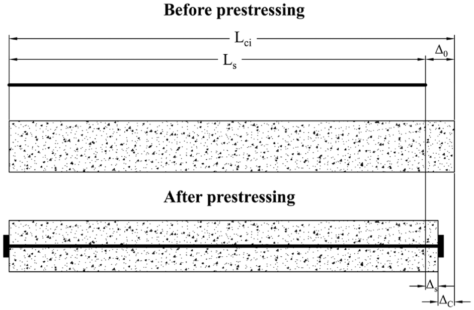
Schematic representation of prestressed concrete beam.

Rewriting equations (1) and (2) in terms of strain yields (3) and (4), respectively, as given below

ε_{C} E_{C} A_{C} = - ε_{S} E_{PS} A_{PS}

(3)

ε_{S} L_{S} - ε_{C} L_{Ci} = Δ_{0}

(4)

where ε_C and ε_S are the strains at the centroids of stiffness of the concrete cross-section and the prestressing strands, respectively, and E_CA_C and E_PSA_PS are the axial stiffnesses of the concrete and prestressing strands, respectively.

Equation (4) represents the compatibility condition at the time of transfer of prestressing. However, it can also be generalized to represent the compatibility condition at any point in time throughout the life of the structure by allowing Δ and L_C to vary with time to reflect changes in the length of the concrete beam caused by rheological strain, as given in equation (5)

ε_{S} L_{S} - ε_{C} L_{C} = Δ

(5)

Eliminating ε_S from equations (5) and (3) through substitution and solving for ε_C yields

ε_{C} = \frac{- Δ}{L_{C} + n L_{S}}

(6)

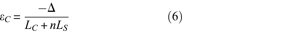
where $n = E_{C} A_{C} / E_{PS} A_{PS}$ .

Eliminating L_C by substituting L_S + Δ, equation (6) can be rewritten as equation (7)

ε_{C} = - 1 + \frac{n + 1}{Δ + L_{S} (n + 1)} L_{S}

(7)

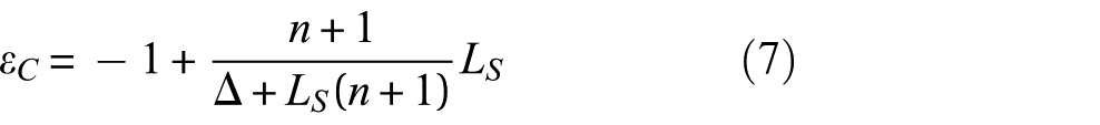
Due to the change in the modulus of elasticity of the concrete during the early-age strength development, equation (7) is rewritten as given in equation (8)

Δ ε_{C} = - 1 + \frac{n (t) + 1}{Δ' (t) + L_{S} (n (t) + 1)} L_{S}

(8)

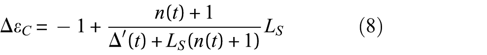
where Δε_C is the change in strain over a short time interval during which the modulus of elasticity is assumed to be constant, $n (t) = (E_{C} (t) A_{C}) / (E_{PS} A_{PS})$ , and Δ′(t) is the change in Δ between two time steps, as given in equation (9).

All variables in equation (8) are based on material or geometrical properties, except for Δ(t) which is determined using strain measurements from the sensors embedded in the concrete and is given by equation (9)

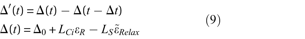
\begin{matrix} Δ' (t) = Δ (t) - Δ (t - Δ t) \\ Δ (t) = Δ_{0} + L_{Ci} ε_{R} - L_{S} {\tilde{ε}}_{Relax} \end{matrix}

(9)

where ε_R is the rheological compressive strain at the centroid of stiffness of the concrete cross-section (negative), and ${\tilde{ε}}_{Relax} = (σ_{Relax} / E_{PS})$ is an equivalent, fictitious tensile strain term that accounts for the change in strain in the centroid of stiffness of the concrete due to strand relaxation, which causes stress loss in the steel, σ_Relax, without strain loss. However, the effect of strand relaxation, which causes stress and force loss, is transmitted to the concrete in terms of strain, effectively changing the length of the concrete beam, much like rheological strain.

Since strain measured by sensors embedded in the concrete is a sum of all strain effects, rheological strain and strain due to stress change caused by strand relaxation cannot be separated. However, since the lengths L_Ci and L_S are approximately equal, L_S can be approximated by L_Ci (steel strands are typically stressed to 0.9f_pu before force transfer, resulting in typical strands elongation of less than 1%, which justifies approximating L_S by L_Ci in equation (9)). Equation (9) can thus be approximated as given in equation (10), where $ε_{R} - {\tilde{ε}}_{Relax}$ is strain measured by the sensors

Δ (t) = Δ_{0} + L_{Ci} (ε_{R} - {\tilde{ε}}_{Relax})

(10)

The initial conditions L_S and Δ₀ can be determined using equation (7) and the measurements from prestressing force transfer, that is, elastic shortening, for ε_C.

The force in the concrete cross-section due to prestressing is then given by equation (11)

F_{C} = \sum_{i = 1}^{m} Δ ε_{C, i} E_{C} (t_{i}) A_{C}

(11)

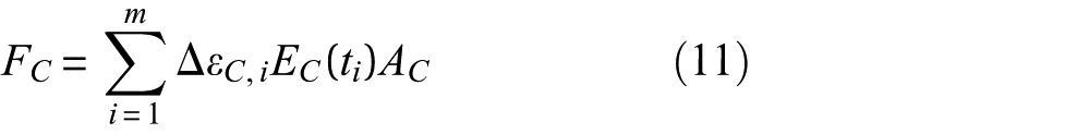
where F is the normal (prestressing) force in the cross-section and t_{1, 2,…, m} are the time steps between which the modulus of elasticity of the concrete is assumed to be constant.

The strain at the centroid of stiffness, used in equation (10), can be determined from measurements within cross-sections. As recommended in the previous section, at least two parallel sensors must be installed at every cross-section. Assuming a linear strain distribution based on linear beam theory, the strain at the centroid of stiffness of the cross-section can be determined as given in equations (12) and (13)

κ = \frac{ε_{b} - ε_{t}}{h}

(12)

ε_{CS} = ε_{t} - κ y_{t, CS}

(13)

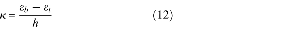
where κ is the curvature of the cross-section, ε_b and ε_t are the measured strains at the top and bottom sensor locations, respectively, h is the vertical distance between the two sensors within the cross-section, ε_CS is the strain at the centroid of stiffness, and y_t,CS is the vertical distance between the top sensor location and the centroid of stiffness of the cross-section.

Since the strain is considered only at the centroid of stiffness, bending effects due to loads are filtered out, and only longitudinal strain remains. In cases of uniaxial bending and assuming no damage to the structure, longitudinal strain only results from thermal effects and the loss of prestressing $(ε_{R} - {\tilde{ε}}_{Relax})$ . Thus, filtering out thermal effects isolates the strain due to rheological effects and strand relaxation required for equation (10).

Since temperature changes can cause significant strain responses in structures, often exceeding responses due to live loads,^19,20 it is important to consider the effects of temperature and to accurately filter out thermal strain. Temperature gradients are typically nonlinear in cross-sections due to several factors such as the effect of heating from the sun (which causes the top of a bridge girder to heat at a faster rate than the bottom) and thermal inertia of concrete. Such temperature effects do not typically equilibrate to steady-state linear gradients.²¹ Therefore, linearly interpolating the temperature at the centroid of stiffness from the temperatures measured at two locations along a cross-section yields an error due to the nonlinear temperature gradient. Moreover, nonlinear temperature gradients create nonlinear stresses in the cross-section that contradict the assumptions of linear beam theory, on which equations (1) through (13) above are based, where linear strain and stress distribution are assumed. Thus, nonlinear temperature effects are filtered in this method by considering only strain measurements from timestamps at which the cross-section considered is under approximately constant temperature, that is, measurements from both temperature sensors in the cross-section are within a specified range. Ideally, considering only strain measurements from timestamps at which the entire structure is under a constant temperature would eliminate all thermal gradients that can cause bending moments or nonlinear strain distributions. However, this criterion might not be feasible, particularly if parts of the structure are exposed to the sun more than others. Thus, the criterion of constant temperature along the cross-section is sufficient since it eliminates deplanation within the cross-section that would contradict the assumptions of linear beam theory and minimizes the error incurred by assuming a linear temperature gradient along the cross-section.

In this study, constant temperature along the cross-section is approximated by a 1°C threshold on the maximum difference between the temperature measurements from the two sensors within the cross-section.²² Then, the effects of constant temperature changes can be compensated for using the concrete thermal expansion coefficient, α_T, as given in equation (14)

ε_{compensated} = ε_{measured} - α_{T} (T_{measured} - T_{ref})

(14)

where ε_compensated is thermally compensated strain, ε_measured is the measured strain, T_measured is the measured temperature at the time of the measured strain, and T_ref is the reference temperature at which strain is assumed to be zero.

After thermal effects are filtered out of strain at the centroid of stiffness of a cross-section, only strain that affects prestress loss (rheological and effect of strand relaxation) remains. In order to compare measurements at different sensor locations and to offset the common issue of missing measurements (see Figure 8), a function is fit to the sensor measurements to better interpolate strain values between measurement sessions and allow for comparisons across sensor locations, where measurements might not be taken at the same time. It is important to note that while models from design codes could have been used to model the strain changes, interpolation functions were chosen instead in order to incorporate the measurements and due to the large uncertainty associated with models from design codes and their parameters. Because seasonal effects remain at the centroid of stiffness caused by changes in bridge column lengths between seasons, changes in the foundation conditions, as well as possible changes in the thermal expansion coefficient, a two-part function is required to account for rheological strain and seasonal effects separately, as given by equation (15). The exponential function is used to approximate the effects of rheological strain due to creep and shrinkage and the effect of strand relaxation, while the sine function approximates the effects of seasonal changes to the structure. Thus, only the first function is used to approximate long-term prestress loss effects. The amplitude of the second function, however, should be used when assessing the integrity of the structure since it can cause variations in the prestressing force seasonally, possibly approaching or exceeding the strength limit state in particular seasons. Due to their seasonal nature, such effects are averaged out over the course of the year. However, if this averaging is not taken into account, the seasonal effects can introduce bias. Thus, they are filtered out in this study by considering only the exponential part of the function. They are later considered separately to differentiate between long-term prestress losses and effects of operational load (seasonal effects)

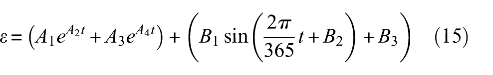
ε = (A_{1} e^{A_{2} t} + A_{3} e^{A_{4} t}) + (B_{1} \sin (\frac{2 π}{365} t + B_{2}) + B_{3})

(15)

where A_1,2,3,4 are the parameters of the exponential function, B_1,2,3 are the parameters of the sine function, and t is the time since prestressing, in days.

It should be noted that strain measurements tend to stabilize over time due to the stabilizing nature of the effects of creep and shrinkage. However, an exponential function, as given in equation (15) or any other function for that matter, will not accurately estimate the time at which the measurements appear to stabilize, instead approaching a limit slower than measurements. Thus, in the interest of accurate representation of the data, the exponential function is assumed to stabilize at the point in time at which its value reaches the average of the last year of measurements. It is represented by a constant value after this time. This is better illustrated through application to field measurements.

Uncertainty analysis

In order to compare measured prestress losses to predicted losses from design codes, uncertainties in the determination of losses from measurements must be considered and rigorously analyzed. The sources of uncertainties are measurement uncertainty and parameter estimation uncertainty. Uncertainties in measurements are related to the monitoring system and supplied by SHM system manufacturers. Uncertainties in parameter estimation include uncertainties in the cross-sectional areas, moduli of elasticity, location of the centroid of stiffness, and lengths of concrete and prestressing steel members. They depend on the methods of estimation or measurement of the parameters and will be discussed in more detail with relation to the application structure in the following sections. It should be noted that the term “uncertainty” in this study represents one standard deviation of a set of repeated measurements as per ISO/IEC.²³

Uncertainties are propagated from measurements and parameters to prestress losses by applying uncertainty propagation formula (16)²⁴ to (11), which leads to the uncertainty given by equation (17). Uncertainties in variables are discussed in more detail through application of the method to the case study structure, as well as in Appendix 1

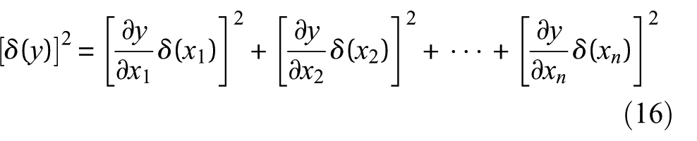
{[δ (y)]}^{2} = {[\frac{\partial y}{\partial x_{1}} δ (x_{1})]}^{2} + {[\frac{\partial y}{\partial x_{2}} δ (x_{2})]}^{2} + \dots + {[\frac{\partial y}{\partial x_{n}} δ (x_{n})]}^{2}

(16)

where y is a function of x₁, x₂, …, x_n and δ(x) is the uncertainty in variable x

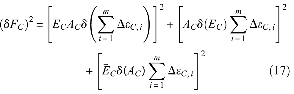
{(δ F_{C})}^{2} = {[{\bar{E}}_{C} A_{C} δ (\sum_{i = 1}^{m} Δ ε_{C, i})]}^{2} + {[A_{C} δ ({\bar{E}}_{C}) \sum_{i = 1}^{m} Δ ε_{C, i}]}^{2} + {[{\bar{E}}_{C} δ (A_{C}) \sum_{i = 1}^{m} Δ ε_{C, i}]}^{2}

(17)

where ${\bar{E}}_{C}$ is the equivalent average modulus of elasticity of the concrete given by ${\bar{E}}_{C} = F_{C} / (A_{C} \sum_{i = 1}^{m} Δ ε_{C, i})$ .

The method described in the previous sections is summarized in Figure 2.

Figure 2.

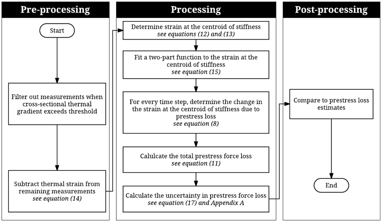
Flowchart of proposed method.

Streicker Bridge

To better illustrate the method, it is presented through application to a segment of Streicker Bridge using a sensor network that was installed during construction. An overview of the structure and its monitoring system are presented in the following sections.

Design

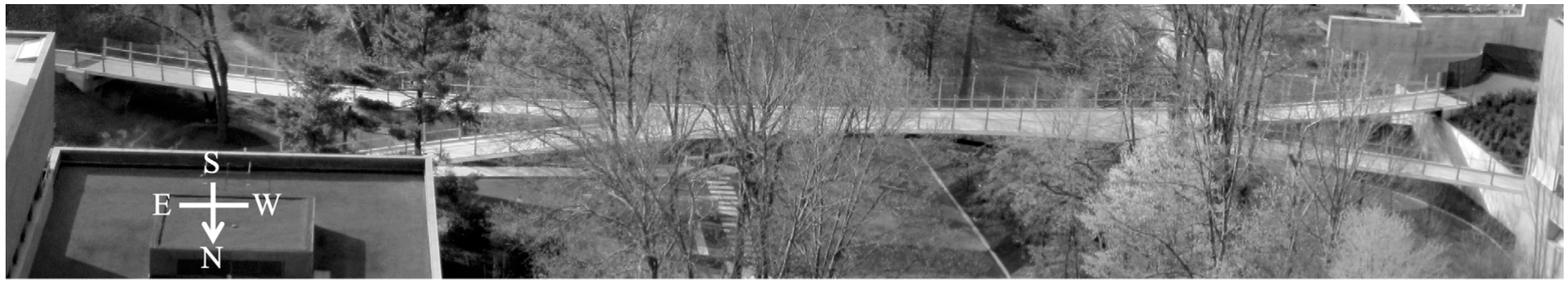
Streicker Bridge is a pedestrian bridge on the Princeton University campus in Princeton, New Jersey, constructed in 2009 and opened in 2010. The bridge is composed of a main span and four approaches, with a total length of 104 m, as shown in Figure 3. The main span’s structural system is a deck-stiffened arch, while the approaches’ are curved continuous girders supported on three Y-shaped columns and an abutment, each. The southeast leg, which is the subject of this study, is shown in Figure 4.

Figure 3.

Top view of Streicker Bridge.

Figure 4.

Southeast leg of Streicker Bridge.

The deck of the bridge is post-tensioned HPC (NJ DOT Class A HPC) with a specified 56-day compressive strength of 6000 psi (42 MPa). The cross-section of the southeast leg is shown in Figure 5. Seven post-tensioning tendons are used for prestressing (numbered 1 through 7 in the figure). Tendons 1, 6, and 7 are Grade III tendons with 6-0.6″ strands each and a jacking force of 277 kips/tendon (1230 kN/tendon). Tendons 2, 3, 4, and 5 are Grade II tendons with 4-0.6″ strands each and a jacking force of 185 kips/tendon (820 kN/tendon). The tendon profiles are shown in Figure 6. Grade 270 low-relaxation strands in accordance with ASTM A416 are used, and all tendons are grouted (Grade C grout). The modulus of elasticity of the strands is given as 28,500 ksi (196 GPa). The 28-day modulus of elasticity of the concrete was estimated using ACI 318-08 section 8.5.1 from compressive strength tests to be 37.5 GPa. The strength evolution of the concrete and its effect on the modulus of elasticity over the first 28 days was taken into account in a previous study.²⁵

Figure 5.

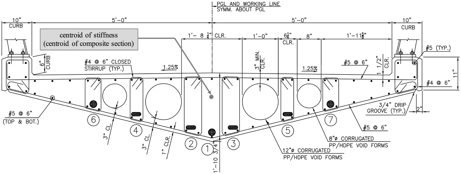
Cross-section of the southeast leg of Streicker Bridge.

Figure 6.

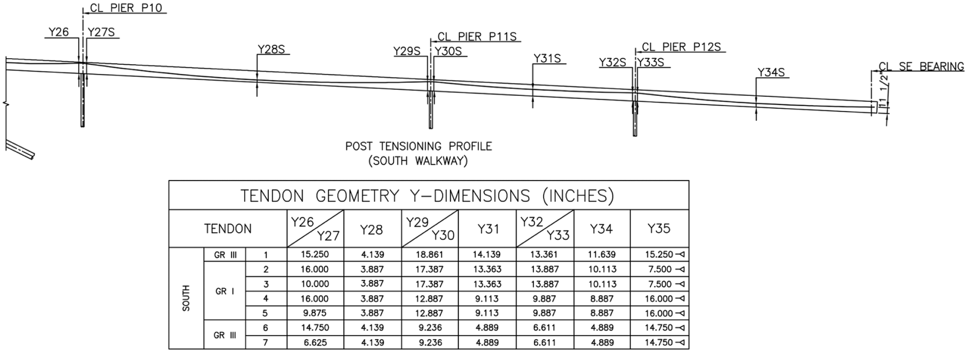
Post-tensioning tendon profile in the southeast leg of Streicker Bridge.

Instrumentation

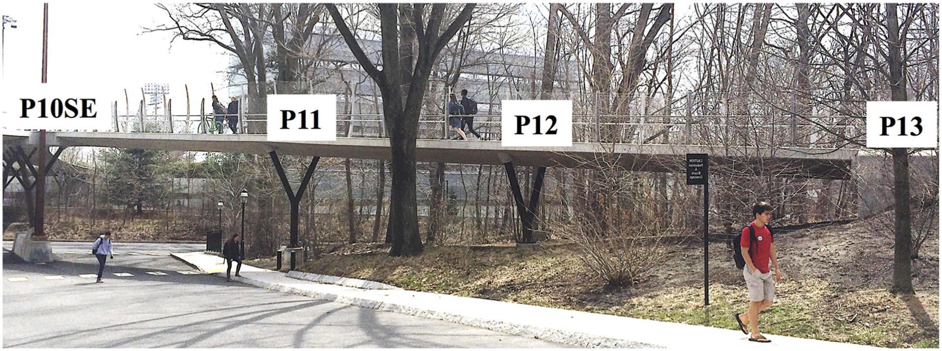
For educational and research purposes, Streicker Bridge was instrumented with a monitoring system during construction. Long-gauge fiber optic strain sensors based on fiber Bragg gratings (FBGs) were loosely attached to reinforcing bars and embedded in the concrete prior to casting. The instrumentation covered half of the main span, along with the southeast leg as it features the longest clear span in the structure (between P10SE and P11, see Figures 4 and 6). This study focuses on the southeast leg and as such, only aspects of the monitoring system pertaining to that segment will be discussed. For more information on the instrumentation of Streicker Bridge, see Sigurdardottir and Glisic.²⁶

In total, 40 temperature and strain sensors are installed in the southeast leg, at the key locations described previously and shown in Figure 7. The sensors are installed in parallel topology, with two sensors at every cross-section installed parallel to each other and to the centerline of the deck. The sensors are installed such that one is closer to the top of the cross-section and one is closer to the bottom of the cross-section. At each of the 18-sensor location, a temperature sensor and a long-gauge strain sensor are installed. Additionally, lateral sensors and sensors with varying gauge lengths are installed for other ongoing research projects and are thus not discussed in this study. All strain sensors have a gauge length of 60 cm, determined based on the recommendations outlined in Glisic.¹⁵

Figure 7.

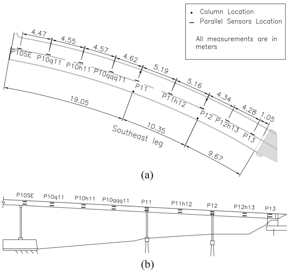
Locations and naming conventions of sensors in the southeast leg: (a) top view and (b) elevation view.

The sensors were installed in October 2009, prior to concrete casting and thus capture the evolution of strain throughout casting, hydration, and prestressing, which took place in two stages, 10 and 11 days after casting. They measure strain and temperature at 5-min intervals when the system is connected. However, the system was often disconnected for use in other research projects. Thus, the data feature gaps.

Method application

Determination of prestress losses

Sample temperature and strain data collected between 2009 and 2016 for the cross-section at P11 (see Figure 6) are presented in Figure 8. Although the datasets feature gaps due to disconnection, the strain data captures casting, post-tensioning, creep and shrinkage, and the effects of seasonal and daily temperature variations at two locations within the cross-section: above the centroid of stiffness (P11up) and below the centroid of stiffness (P11down).

Figure 8.

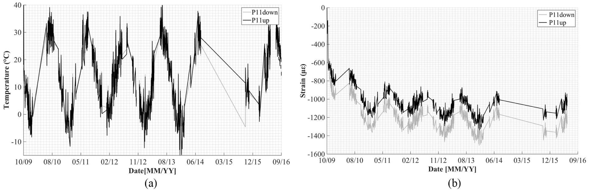
Sample data from location P11 from: (a) temperature sensors and (b) strain sensors.

Using measurements from pairs of sensors, such as in Figure 8, first, thermal effects are filtered out by considering only points in time where measurements from the two sensors within the cross-section are approximately equal (i.e. within a 1°C threshold in this study). Figure 9 shows the temperature difference measurements between the top and bottom sensors at the cross-section at P11. Approximately, 47% of the data falls within the ±1°C thresholds. Temperature measurements recorded by the two sensors can be significantly different; Figure 9 shows up to an 8°C difference for the two sensors in the cross-section at P11 where sensors are 370 mm apart.

Figure 9.

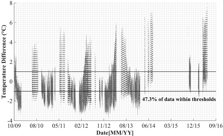
Temperature difference between the two sensors installed at location P11.

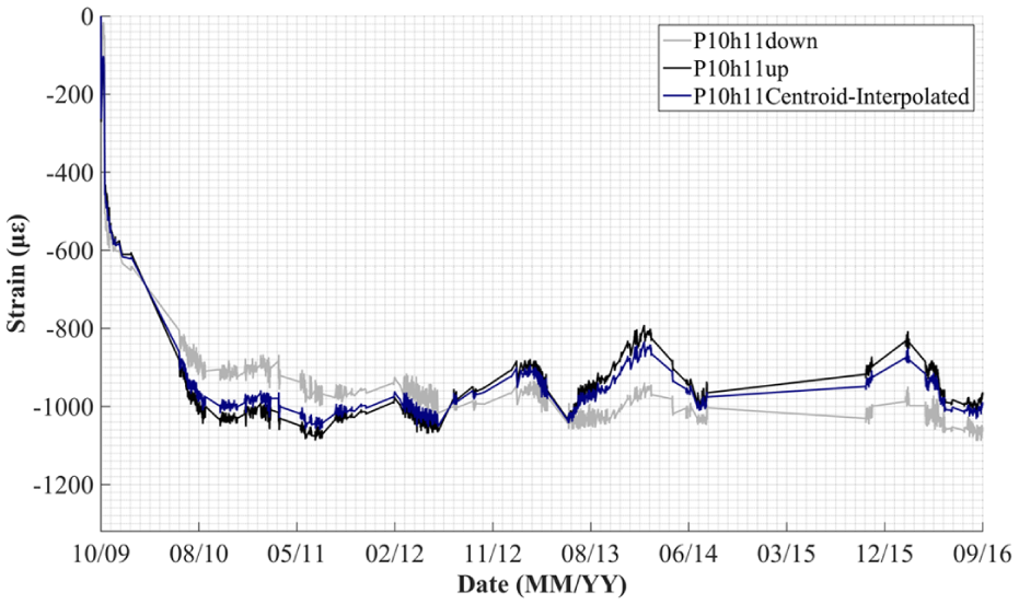
Using the remaining strain measurements, thermal strain is compensated for using equation (14) and a thermal expansion coefficient of 10 με/°C, as determined in a previous study.²⁷ An illustration of the result is shown in Figure 10, with thermally compensated strain measurements from the two sensors at location P11, in addition to the strain at the centroid of stiffness of the cross-section. Similar diagrams are obtained for all other locations, as shown in Appendix 2. The location of the centroid of stiffness was determined experimentally using strain measurements during form removal when the dead load was applied to the structure. More detail regarding this procedure is found in Sigurdardottir and Glisic.²⁶

Figure 10.

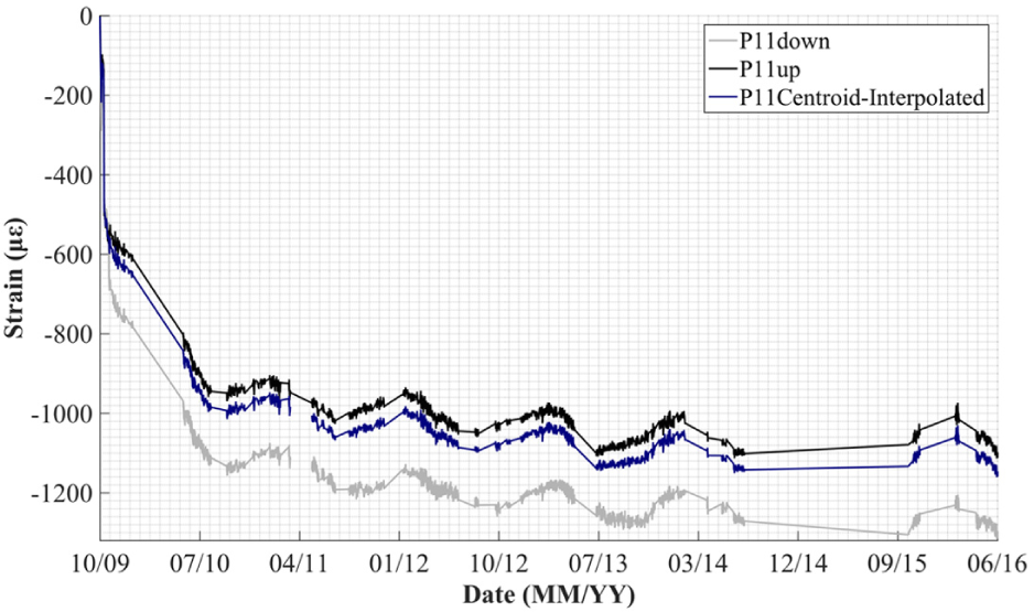
Temperature-compensated strain measurements at location P11.

A function of the form given in equation (15) is then fit to the interpolated measurements for the centroid of stiffness, as shown in Figure 11. Although thermal strain is filtered out, some seasonal influences remain, as shown in Figures 10 and 11, these influences are due to the effect of the average temperature on foundations, the soil surrounding the structure, and the column supports, as well as due to potential variation of thermal expansion coefficient over the year. Figure 11 also shows the function that approximates the measurements (gray), as well as the part of the function that approximates non-seasonal trend, that is, rheological and strand relaxation effects (black). The sinusoidal curve serves to approximate the seasonal effects (operational load) and is thus irrelevant to prestress loss calculation, as it does not reflect long-term changes in the dimensions of the concrete beam. As an example, the parameters of the models shown in Figure 11 are as follows: A₁ =−1026.0, A₂ = 3.58 × 10^–5, A₃ = 508.1, A₄ =−5.93 × 10^–3, B₁ = 37.1, B₂ = –0.99, and B₃ =−0.35. The average uncertainty of the model (average of the difference between the model and measurements) is approximately 18 με. The same procedure was applied and model parameters determined for all other locations and then used in determination of prestress losses for each location as described below. Note that the model parameters are different at every sensor location due to the different initial force and creep parameters.

Figure 11.

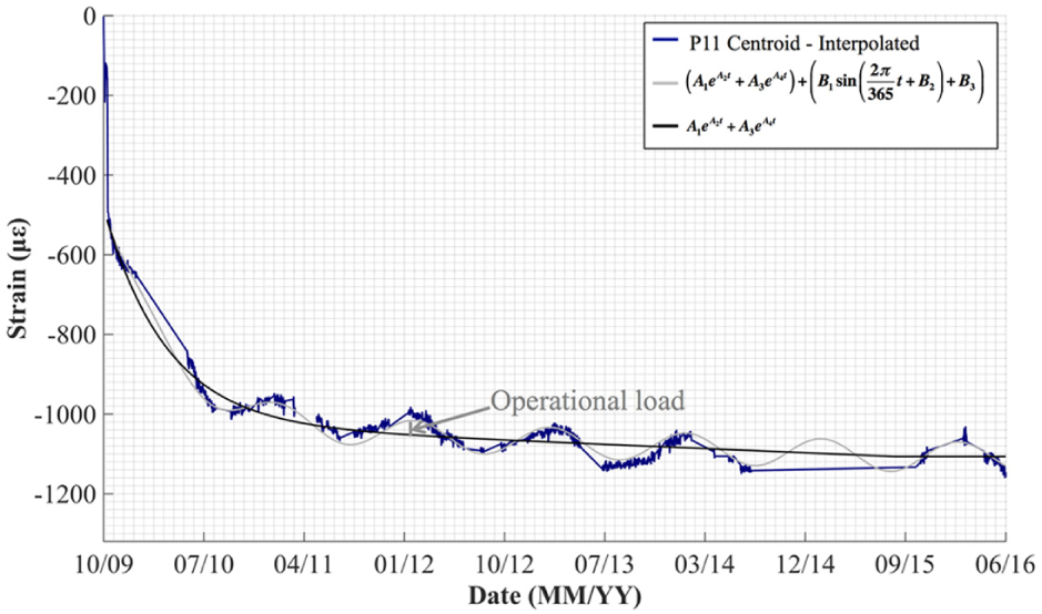
Interpolated measurements at the centroid of stiffness of the cross-section at P11 and approximating functions for overall behavior (gray) and rheological strain (black).

As previously mentioned, the exponential model given in equation (15) stabilizes slower than the actual measurements do. Thus, it is assumed to stabilize at the point in time at which its value reaches the average of the last year of measurements, August 2015 in this case. Measurements are assumed to be constant after this point in time.

Using the function shown in Figure 11 and equations (8), (10), and (11), the absolute magnitude of the force from the time of transfer (i.e. post-tensioning) can be approximated. Figure 12 shows the results at location P11 using the data over 7 years. As shown in Figure 12, a significant percentage of the force loss (around 70% of total loss) is due to immediate losses caused by friction, anchorage loss, and elastic shortening. As for long-term prestress losses due to rheological strain and strand relaxation, they constitute approximately 8% of total prestressing force, a significant proportion of which (more than 50%) occurs during the first 6 months, as shown in Figure 14.

Figure 12.

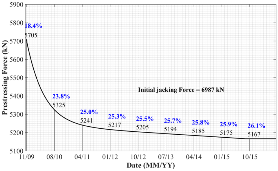
Prestressing force loss between 2009 and 2016 at location P11 (force loss as a percentage of initial jacking force is shown in blue at 9-month intervals).

The behavior shown in Figures 10 through 12 for location P11 matches predicted behavior, that is, increasing compressive strain in the concrete that stabilizes over time. Other locations along the bridge, however, exhibit unusual behavior approximately 3 years after construction, where strain at one of the sensor locations within a cross-section increases over time. An example of this behavior is shown in Figure 13. This has been attributed to probable settlement of foundations, particularly at the abutment location P13 and the foundation under column P10 (see Figures 4 and 7). This behavior is the subject of ongoing research on the structure and is beyond the scope of this study. Since this behavior is not well understood yet, measurements are analyzed for the first 3 years to estimate prestress losses for this study.

Figure 13.

Temperature-compensated strain measurements at location P10h11.

Data for two locations, P10qqq11 and P11, do not exhibit this irregular behavior, and they are analyzed first to understand the evolution of long-term prestress losses and approximate the percentage of losses that occurs over the first 3 years. Figure 14 shows the evolution of long-term losses at locations P10qqq11 and P11. As shown, more than 90% of long-term losses can be approximated using data from the first 3 years.

Figure 14.

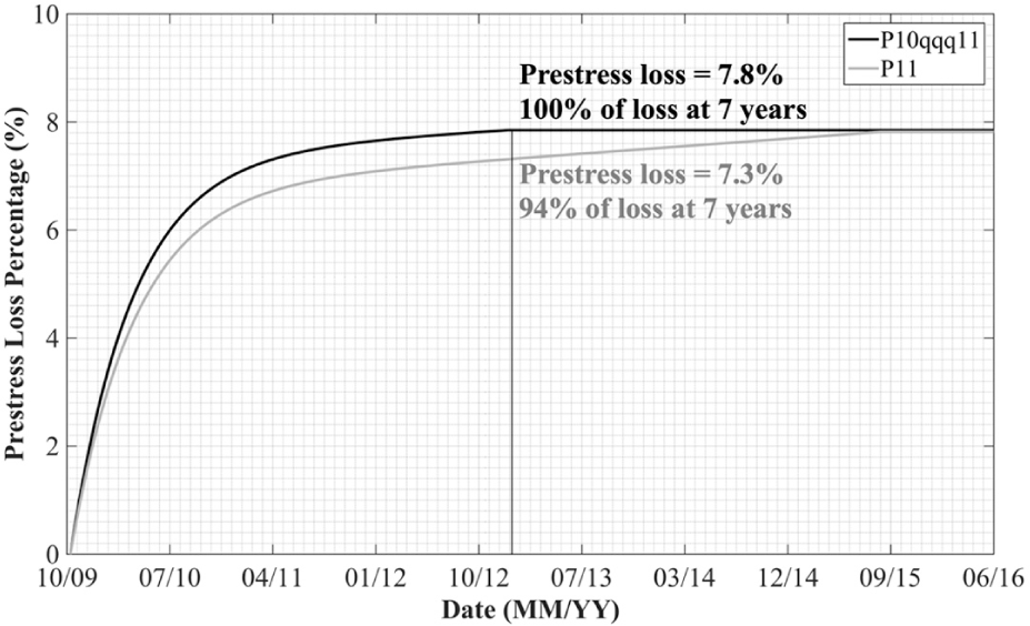
Evolution of long-term prestress losses at locations P10qqq11 and P11 as a percentage of jacking force.

Using available measurements, the prestressing force loss during the first 3 years is estimated at every instrumented cross-section as previously outlined in section “Method for monitoring long-term prestress losses.” The results are presented in Figure 15, with estimates plotted every month for the first 3 years after transfer of prestressing. The prestressing force loss decreases over time as illustrated by the change in the density of lines as time progresses.

Figure 15.

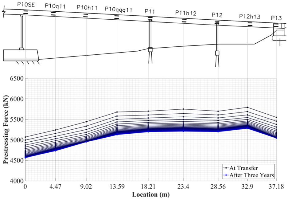
Prestressing force loss over 3 years (2009–2012) plotted every month (black to blue transition designates date).

Quantification of uncertainties in prestress losses

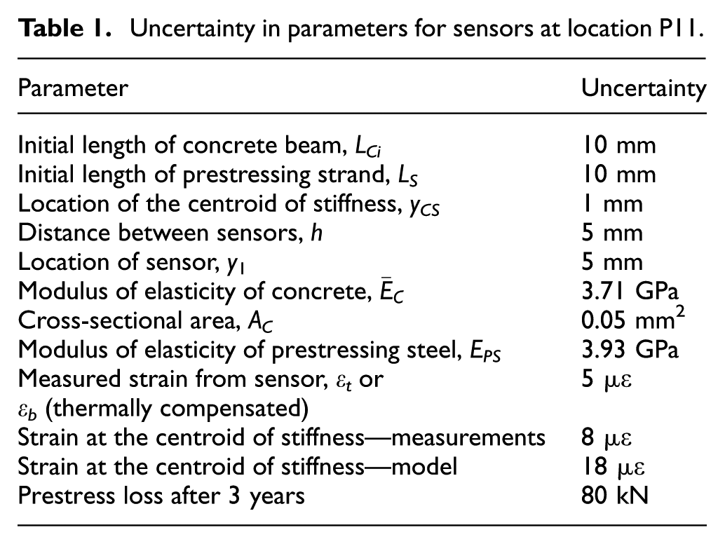
Uncertainties in prestress losses were determined as outlined previously and Appendix 1. As an example, the parameter uncertainty and prestress loss uncertainty for location P11 is given in Table 1. Uncertainties in dimensions, cross-sectional area, and sensor locations are based on construction tolerances, while uncertainty in the location of the centroid of stiffness is determined experimentally as discussed in Sigurdardottir and Glisic.²⁶ Uncertainty in the modulus of elasticity of concrete is assumed to be 10% based on ACI 318-08 section 8.5.1 commentary (more details provided in Appendix 1), while uncertainty in the modulus of elasticity of the prestressing strands is assumed to be 2% (assumed based on experience, since no value was provided by manufacturer). Strain measurements uncertainty is based on specifications of the manufacturer of the monitoring system. The uncertainty in the model is the average deviation of measurements from the model, as shown in Figure 11. Prestress losses were similarly determined for every sensor location. Figure 16 shows the results for the final prestressing force distribution after 3 years along with the 80% confidence interval based on determined uncertainties.

Figure 16.

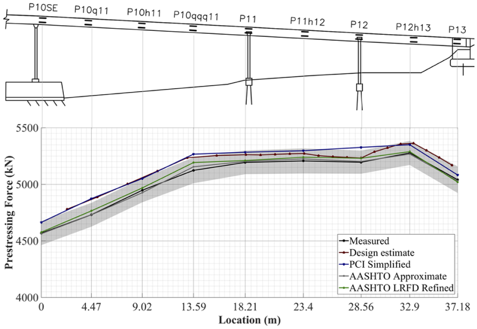
Prestressing force distribution after 3 years (2009–2012) with 80% confidence interval and four estimates for prestress losses.

Table 1.

Uncertainty in parameters for sensors at location P11.

Parameter	Uncertainty
Initial length of concrete beam, L_Ci	10 mm
Initial length of prestressing strand, L_S	10 mm
Location of the centroid of stiffness, y_CS	1 mm
Distance between sensors, h	5 mm
Location of sensor, y₁	5 mm
Modulus of elasticity of concrete, ${\bar{E}}_{C}$	3.71 GPa
Cross-sectional area, A_C	0.05 mm²
Modulus of elasticity of prestressing steel, E_PS	3.93 GPa
Measured strain from sensor, ε_t or ε_b (thermally compensated)	5 µε
Strain at the centroid of stiffness—measurements	8 µε
Strain at the centroid of stiffness—model	18 µε
Prestress loss after 3 years	80 kN

Comparison to code estimates

The final prestressing force distribution after 3 years, associated uncertainties, and four prestress loss estimates are presented in Figure 16. The first estimate is provided by the designer of the structure and is based on CEB-FIP model for shrinkage and creep calculations²⁸ and on AASHTO LRFD Refined estimate for strand relaxation.²⁹ Other estimates used are based on recommendations in the Guide to Estimating Prestress Loss, a report by Joint ACI-ASCE Committee 423.¹⁰ Three of the four estimates outlined in the report are calculated and presented here: PCI Simplified Method,³⁰ AASHTO Approximate Method,²⁹ and AASHTO LRFD Refined Method.²⁹ All four estimates yield comparable results as shown in Figure 16 and Table 2.

Table 2.

Measured prestressing force loss and estimates using PCI simplified method, AASHTO approximate method, AASHTO LRFD method, and designer estimate.^a

	P10SE	P10q11	P10h11	P10qqq11	P11	P11h12	P12	P12h13	P13
Measured loss (kN)	499.9	509.5	493	554.3	504.6	542	502.4	514.6	508
Uncertainty (kN)	81.6	80.9	81.9	87.6	80.1	85.7	78.2	82.0	90.1
PCI simplified estimate (kN)	411.0	374.0	398.7	419.3	422.4	461.1	378.8	451.1	473.9
Confidence level	28%	9%	25%	12%	31%	34%	11%	44%	71%
AASHTO approximate estimate (kN)	511.8	517.1	523.5	531.2	503.4	533.3	503.4	533.9	526.6
Confidence level	88%	93%	71%	79%	99%	92%	99%	81%	84%
AASHTO LRFD refined estimate (kN)	498.0	482.2	481.4	493.5	495.6	518.5	475.2	512.2	536.6
Confidence level	98%	74%	89%	49%	91%	78%	73%	98%	75%
Design estimate^a (kN)	413.5	384.0	395.0	426.1	444.9	484.5	473.0	421.3	416.9
Confidence level	29%	12%	23%	14%	46%	50%	71%	26%	31%

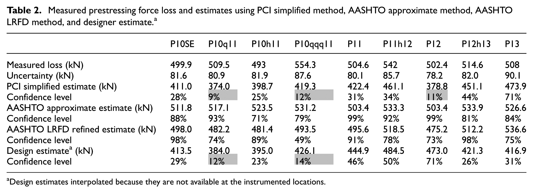
Design estimates interpolated because they are not available at the instrumented locations.

The results show that the code estimates for time-dependent prestress losses are mostly within the 80% confidence interval of measured losses, with a few exceptions. This indicates that measured prestress losses do not significantly exceed design estimates. It is interesting to note that the estimates using AASHTO Approximate Method and AASHTO LRFD Refined Method yield slightly more conservative results than the estimates from the designer and using the PCI Simplified Method.

Additionally, confidence levels are calculated and presented in Table 2 for each of the four estimates at each of the nine instrumented locations. The confidence levels represent the probability that the measured prestress loss and the estimate are not different and are calculated based on a Gaussian probability density function with the measured prestress loss value as the mean and the uncertainty as the standard deviation. The following thresholds on confidence levels are proposed for two-tailed analysis:

≤2%: there is a highly significant difference between the measured loss and the estimate;

≤10%: there is a significant difference between the measured loss and the estimate;

≤20%: there is a marginally significant difference between the measured loss and the estimate;

>20%: there is no significant difference between the measured loss and the estimate.

The confidence level threshold of 20% was proposed and used in a previous study.²⁵ It is higher than typical confidence levels of 5% (corresponding to a 95% confidence interval) due to the fact that there are unknown uncertainties associated with prestress loss estimates. Highlighted cells in Table 2 represent values that are below the threshold. While most confidence levels exceed the 20% threshold, some are below. Those correspond to measured prestress losses compared to PCI Simplified Method estimates and the designer estimate. This further shows that measured losses are in agreement with predicted values, but predictions are not overly conservative.

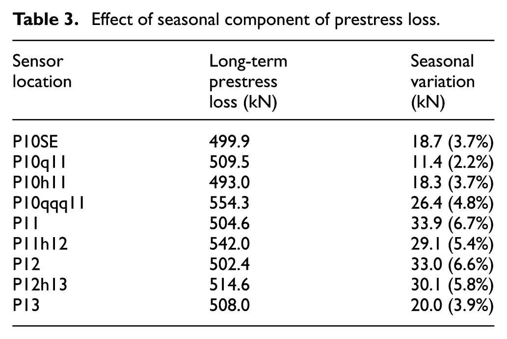
As previously mentioned, seasonal variations in temperature and humidity cause strain changes in the structure as shown in Figures 5 and 6. While these effects have been disregarded in the analysis, it is important to quantify their impact on the variation of prestressing forces. Table 3 presents the seasonal component of the prestressing force variation at every instrumented location of the southeast leg of Streicker Bridge, as well as the long-term (non-seasonal) prestress loss for comparison. As shown in Table 3, the effects are more pronounced in the shorter spans, possibly because the structure is more restrained to thermal effects. Overall, seasonal effects are less than 7% of long-term prestress losses.

Table 3.

Effect of seasonal component of prestress loss.

Sensor location	Long-term prestress loss (kN)	Seasonal variation (kN)
P10SE	499.9	18.7 (3.7%)
P10q11	509.5	11.4 (2.2%)
P10h11	493.0	18.3 (3.7%)
P10qqq11	554.3	26.4 (4.8%)
P11	504.6	33.9 (6.7%)
P11h12	542.0	29.1 (5.4%)
P12	502.4	33.0 (6.6%)
P12h13	514.6	30.1 (5.8%)
P13	508.0	20.0 (3.9%)

Conclusion

Monitoring of prestressed concrete structures is important as the use of prestressed concrete continues to increase, particularly in conjunction of new materials, such as HPC, that exploit the benefits of prestressed construction. This article presents a comprehensive SHM method for the monitoring of prestress loss and the long-term distribution of prestressed forces in beam-like structures. The method is based on the use of strain measurements from long-gauge fiber optic sensors embedded in the concrete before casting. Its strengths include (1) robustness to effects of operational load, including seasonal variations, due to the focus on the strain at the centroid of stiffness; (2) quantification of uncertainties, which enables probabilistic comparison to design estimates; and (3) applicability to different classes of beam-like structures beyond bridge girders. The method was applied to measurements from Streicker Bridge, a pedestrian bridge in Princeton, New Jersey, collected over 7 years since the construction of the structure in 2009. Results from the analysis indicate that design estimates are not necessarily conservative but are generally close to the prestress losses obtained using sensor measurements. Additionally, the results from this study on Streicker Bridge show that most time-dependent prestress losses in the structure occur during the first 3 years (94%–100% in this case).

Although previous studies indicate that prestress losses in HPC are lower than losses in traditional concrete, the results from this case study indicate that it is not necessarily the case, as also analytically discussed in Barr et al.,¹² where the magnitude of losses in HPC was found to be dependent on other characteristics of the concrete mix causing prestress losses to be higher or lower in HPC than in traditional concrete. This result suggests the importance of monitoring prestressed concrete structures rather than drawing generalized conclusions about all structures based on characteristic studies.

Footnotes

Appendix 1

Appendix 2 Acknowledgements

The Streicker Bridge project has been realized with the great help and kind collaboration of several professionals and companies. We would like to thank Steve Hancock and Turner Construction Company; Ryan Woodward and Ted Zoli, HNTB Corporation; Dong Lee and A G Construction Corporation; Steven Mancini and Timothy R Wintermute, Vollers Excavating and Construction, Inc.; SMARTEC SA, Switzerland; Micron Optics, Inc., Atlanta, GA; Geoffrey Gettelfinger; James P Wallace; Miles Hersey; Paul Prucnal; Yanhua Deng; Mable Fok; and Faculty and staff of the Department of Civil and Environmental Engineering. The following students installed the sensors on Streicker Bridge: Chienchuan Chen, Jeremy Chen, Jessica Hsu, George Lederman, Kenneth Liew, Maryanne Wachter, Allison Halpern, David Hubbell, Morgan Neal, Daniel Reynolds, and Daniel Schiffner. Special thanks to Dorotea Sigurdardottir for the permission to use her drawings and to Prof. Matthew Yarnold (Tennessee Technological University) and Jack Reilly for the information regarding work on temperature-driven SHM.

Declaration of conflicting interests

The author(s) declared no potential conflicts of interest with respect to the research, authorship, and/or publication of this article.

Funding

The author(s) disclosed receipt of the following financial support for the research, authorship, and/or publication of this article: This work was partially supported by the National Science Foundation (Grant No. CMMI-1362723). Any opinions, findings, and conclusions or recommendations expressed in this paper are those of the authors and do not necessarily reflect the views of the National Science Foundation. The work was also supported by USDOT Office of the Assistant Secretary for Research and Technology (Grant No. DTRT13-G-UTC28). The views, opinions, findings, and conclusions are the responsibility of the authors only and do not represent the official policy or position of the USDOT or any state or entity.

References

Garber

Gallardo

Deschenes

et al . Experimental investigation of prestress losses in full-scale bridge girders. ACI Struct J 2015; 112(5): 553–564.

Idriss

Solano

. Effects of steam curing temperature on early prestress losses in high-performance concrete beams. J Transp Res Board 2002; 1813(1): 218–228.

Glisic

Inaudi

. Fibre optic methods for structural health monitoring. Chichester: John Wiley & Sons, 2007.

Saiidi

Douglas

Feng

. Prestress force effect on vibration frequency of concrete bridges. J Struct Eng 1994; 120(7): 2233–2241.

Noble

Nogal

O’Connor

et al . The effect of post-tensioning force magnitude and eccentricity on the natural bending frequency of cracked post-tensioned concrete beams. J Phys Conf Ser 2015; 628: 12047.

Fabo

Jarosevic

Chandoga

. The smart tendons—a new approach to prestressing. In: Proceedings of the fib symposium 2004—concrete structures: the challenge of creativity, Avignon, 26–28 April 2004.

Liu

. A novel integrated sensor for stress measurement in steel strand based on elastomagnetic and magnetostrictive effect. In: Peter WT et al. (eds) Engineering asset management—systems, professional practices and certification, lecture notes in mechanical engineering. Cham: Springer, 2015, pp. 65–73.

Lanza di Scalea

Rizzo

Seible

. Stress measurement and defect detection in steel strands by guided stress waves. J Mater Civil Eng 2003; 15(3): 219–227.

Chaki

Bourse

. Stress level measurement in prestressed steel strands using acoustoelastic effect. Exp Mech 2009; 49(5): 673–681.

10.

Joint ACI-ASCE Committee 423. Guide to estimating prestress loss. Farmington Hills, MI, 2016, https://www.concrete.org/Portals/0/Files/PDF/Previews/423.10R-16_preview.pdf

11.

Stallings

Barnes

Eskildsen

. Camber and prestress losses in Alabama HPC bridge girders. PCI J 2003; 48(5): 90–104.

12.

Barr

Eberhard

Stanton

et al . High performance concrete in Washington State SR18/SR516 overcrossing: final report on girder monitoring. Report for Washington State Transportation Commission, December2000, http://depts.washington.edu/trac/bulkdisk/pdf/477.1.pdf

13.

Dwairi

Wagner

Kowalsky

et al . Behavior of instrumented prestressed high performance concrete bridge girders. Constr Build Mater 2010; 24(11): 2294–2311.

14.

Kamatchi

Dhayalini

Balaji Rao

et al . Estimation of long-term prestress losses of box-girder bridge span using the prestress loss models in Indian and International codes of practices and comparison with field measurements. Indian Concr J 2015; 89(5): 59–68.

15.

Glisic

. Influence of the gauge length on the accuracy of long-gauge sensors employed in monitoring of prismatic beams. Meas Sci Technol 2011; 22(3): 35206.

16.

Sigurdardottir

Glisic

. Neutral axis as damage sensitive feature. Smart Mater Struct 2013; 22(7): 75030.

17.

Abdel-Jaber

Glisic

. Analysis of the status of pre-release cracks in prestressed concrete structures using long-gauge sensors. Smart Mater Struct 2015; 24(2): 25038.

18.

Pozzi

Zonta

et al . Development and laboratory validation of in-line multiplexed low-coherence interferometric sensors. Opt Fiber Technol 2008; 14(4): 281–293.

19.

Catbas

Aktan

. Condition and damage assessment: issues and some promising indices. J Struct Eng 2002; 128(8): 1026–1036.

20.

Beskhyroun

Wegner

Sparling

. New methodology for the application of vibration-based damage detection techniques. Struct Control Hlth 2012; 19(8): 632–649.

21.

Emanuel

Hulsey

. Temperature distributions in composite bridges. J Struct Div: ASCE 1978; 104: 65–78.

22.

Reilly

Abdel-Jaber

Yarnold

et al . Identification of steady-state uniform temperature distributions to facilitate a temperature driven method of Structural Health Monitoring. In: Proceedings of SPIE 9805: health monitoring of structural and biological systems, Las Vegas, NV, 24 March 2016.

23.

ISO/IEC. International vocabulary of metrology—basic and general concepts and associated terms, 3rd ed. VIM, ISO/IEC Guide 99-12:2007. Geneva: International Organization for Standardization, 2007.

24.

Rabinovich

. Measurement errors and uncertainties, theory and practice, 3rd ed. New York: Springer, 2005.

25.

Abdel-Jaber

Glisic

. A method for the on-site determination of prestressing forces using long-gauge fiber optic strain sensors. Smart Mater Struct 2014; 23(7): 75004.

26.

Sigurdardottir

Glisic

. On-site validation of fiber-optic methods for structural health monitoring: Streicker Bridge. J Civ Struct Heal Monit 2015; 5(4): 529–549.

27.

Ditchfield

. Monitoring temperature effects on Streicker Bridge using fiber optic sensors. Princeton, NJ: Princeton University, 2013.

28.

Comite Euro-International du Beton. CEB-FIP model code 1990. London: Thomas Telford Services, 1993.

29.

AASHTO. AASHTO LRFD bridge design specifications, 6th ed.Washington, DC: American Association of State Highway and Transportation Officials, 2012, 1661 pp.

30.

Prestressed Concrete Institute (PCI). PCI design handbook, 7th ed.Chicago, IL: Precast/Prestressed Concrete Institute, 2010, 804 pp.