
Abstract
Structural health monitoring plays an increasingly significant role in detecting damages for large and complex structures to ensure their serviceability and sustainability. Optimal sensor placement is critical in the structural health monitoring system as the sensor configuration directly impacts the quality of collected data used for structural health diagnosis. Therefore, this study presents a comprehensive review of computational methodologies for optimal sensor placement in structural health monitoring. The problem formulation of optimal sensor placement is first introduced, including commonly used evaluation criteria for sensor configurations. Then, various existing optimization methodologies for sensor placement are summarized and introduced in detail, especially for the evolutionary algorithms and their improved variants. Finally, the suitability of computational methods for specific structural health monitoring applications is also discussed. The main goal of this study is to deliver a comprehensive reference of computational methodologies for optimal sensor placement in structural health monitoring studies and applications. This article is concluded by highlighting the most widely utilized evaluation criteria and optimization methodologies for sensor configuration determination.
Keywords
Introduction
Structural health monitoring (SHM) is defined as the process of implementing strategies to detect damages for the structures of civil, aerospace, and mechanical engineering1–3 to guarantee their serviceability and sustainability. SHM has been widely used for the past decades as the increasing number of large and complex structures was constructed worldwide. Brownjohn 4 and Karbhari and Ansari 5 discussed the motivations for and the development of SHM applications to different categories of civil infrastructure in the 20th century. Case studies on specific types of structure are also provided for illustration.
A typical SHM system consists of sensors, data collection and transmission subsystem, a database for data management, and health diagnosis. 6 One critical technology involved in an SHM system is sensing technology, which is not limited to SHM applications but has been applied in many fields such as structural design, 7 construction progress monitoring, 8 safety risk,9–11 and smart operation and maintenance management. 12 Ou and Li 6 reviewed the development of advanced sensing technologies and sensors in mainland China. Sensors are usually fundamental elements in the SHM system. The sensors in the SHM are utilized not only to monitor the structural status, such as stress and displacement, but also to monitor the environmental parameters, such as the temperature and wind speed which are impacting the structures. 13 For example, Ansari 14 introduced basic principles related to practical health monitoring of large civil structures with optical fiber sensors, where the sensor packaging, sensor placement, strain transfer mechanism, and sensor reliability were discussed.
Sensors are generally divided into two types, namely wired and wireless sensors. Wired sensors are usually limitedly applied since they require to be installed during structure construction, and the wiring might potentially impact the function of the structure with a limited number of sensors. 15 Therefore, with the development of wireless sensors, wireless monitoring has emerged in recent years as a promising technology that could significantly impact SHM.16,17 The development of wireless sensors and sensor networks for SHM was reviewed by Lynch and Loh. 18 In this review, the hardware architecture is identified as a critical element in wireless sensors design for SHM. In addition, the advantages (e.g. automated detection through the collocation of computational power with the sensing transducer) and disadvantages (e.g. finite energy sources) of wireless sensor networks (WSNs) are also discussed. 19 WSNs have already been deployed in several fields. For example, Xu et al. 20 described the design and deployment of a WSN for structural monitoring. Jang et al. 21 illustrated the deployment and evaluation of a state-of-the-art WSN on a cable-stayed bridge named Jindo Bridge in South Korea, which was newly constructed with a 344 m main span and two 70 m side spans.
Sensor placement, also named as sensor deployment 22 or sensor configuration, is always the basic process of constructing the sensor network for an SHM system. Besides, SHM allows an optimal usage of the structure, a minimized downtime, and the avoidance of catastrophic failures, helps improve the product design, and completely changes the approach to conducting maintenance activities. Therefore, optimizing the sensor configuration for SHM requires considering more aspects compared to other optimization problems. On one hand, the optimization of sensor placement needs to meet the requirements of SHM. One the other hand, an optimal sensor configuration requires minimizing the number of sensors required and increasing the accuracy of data collection and provides a powerful SHM system. 23 Several studies have explored the sensor placement optimization. For example, Younis and Akkaya 24 introduced the current state of studies on optimizing the sensor placement in WSN, where the placement strategies were divided into static and dynamic based on whether the optimization was conducted during the sensor deployment or at the operation stage of networks. Guerriero et al. 25 discussed the determination of sensor configuration by displacing sensors from an initial sensor configuration. In addition, Abdollahzadeh and Navimipour 22 conducted a comprehensive review of deployment strategies in WSN. However, a comprehensive review of the optimal sensor placement (OSP) problem and related computational methodologies used for OSP is still lacking.
Considering the importance of SHM for the increasing number of large complex structures around the world and the impact of sensor configurations on SHM performance, this study aims at delivering a comprehensive review on the OSP problem and related computational methodologies used in sensor placement optimization, including both wired and WSN configurations. Furthermore, the reviewed results of this study are expected to provide an effective reference to sensor configuration determination for SHM system construction.
The rest of this study is organized as follows. Section “Problem formulation” formulates the sensor placement optimization problem, including problem description and the commonly used evaluation criteria. Optimization computational methodologies by category are introduced in section “Optimization methodologies.” Section “Conclusion” concludes this study.
Problem formulation
Degree of freedom and finite element model
As aforementioned, SHM mainly aims at monitoring and detecting structural damages, from materials to structural stability. Instability of a structure originates from the displacement at the joints of the structure. Degree of freedom (DOF) indicates the degrees of freedom (e.g. move or rotate) that any particular joint contains. A DOF of a certain structure denotes the number of directions that the structure can generate displacement at a joint. Therefore, the positions of joints or DOFs can be used as candidate locations to install proper sensors to enable data collection for structural damage monitoring and detection.
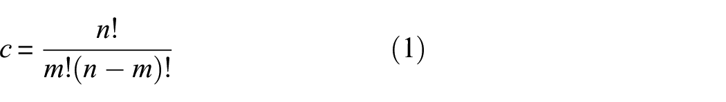
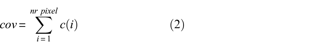
Methodologies of sensor configuration determination vary among different structures. For simple and regular structures or smaller number of DOFs, such as steel frame in real harsh environment,26,27 cables in post-tensioned members, 14 scaled-down transmission tower, 28 and simple building structures,29,30 physical sensors (wired or wireless) can be installed for data collection and validate different sensor configurations for the target structures. However, SHM is more commonly applied in large and complex structures for damage detection or structural state monitoring. For these structures, such as large buildings, towers with an irregular shape, and long-span cable-stayed bridges (see Figure 1), the numerical experiment is preferred, because the unlimited sensor configuration can be efficiently and economically tested. Three-dimensional finite element (FE) models 31 are usually required to be constructed for the numerical experiment to optimize the sensor placement.
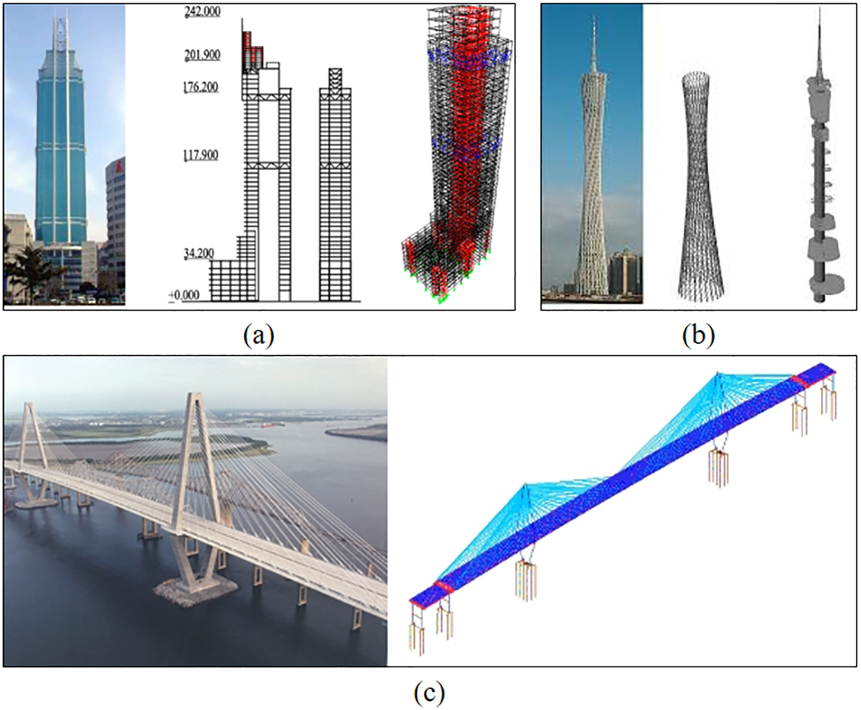
Illustration of real structures to FE models: (a) large building, (b) tower with irregular shape, and (c) long-span cable-stayed bridge.
The generated FE models may have thousands of DOFs given the complexity of the large structure. Therefore, model simplification and reduction methods are usually required to efficiently determine the sensor configuration. For example, Ni et al. 32 established an equivalent reduced-order FE model for Canton Tower, which contained 37 beam elements and a total of 185 DOFs. Yi et al. 33 also used this established FE model for sensor configuration study on the Canton tower using various evolutionary algorithms.
To generate three-dimensional (3D) FE models for OSP, many computational applications can be utilized. The most widely used application among OSP studies is ANSYS.7,28,33–41 For example, Yi et al. 33 used ANSYS to construct an FE model for Canton Tower, where the 3D full-order FE model contained 84,370 nodes and 505,164 DOFs. Xu et al. 39 created the FE model of the physical Tsing Ma Bridge using ANSYS. Chow et al. 28 used ANSYS to construct the FE model for the transmission tower. In addition to ANSYS, other FE analysis software, such as SAP,31,42 SAFESA™, 43 Grillage, 44 Autodesk Simulation Multiphysics, 45 ETABS, 46 FLAC3D, 47 and ABAQUS, 26 are also available for FE model generation.
OSP problem description
Since OSP mainly aims at determining the DOFs for sensor installation, most of the sensor placement optimization can be summarized as “given a set of
where
For most studied structures,
In addition to global SHM, where low-frequency guided waves are mainly employed, as mentioned above, OSP has also been applied to ultrasonic testing, where nondestructive examination (NDE) techniques that use short, high-frequency ultrasonic waves to identify flaws in material or damages in a structural component.51–54 For the ultrasonic NDE, usually the maximum value of coverage by the sensors or transducers is formulated as the fitness function to determine the sensor placement. 55 Actuator–sensor pairs usually obtain binary images of the sensor network system, where 0 and 1 values are included. Then, all these images are summed to evaluate the performance of the actuator–sensor network system. For example, Thiene et al.49 defined the coverage fitness function as
where
Evaluation criteria
As mentioned in section “OSP problem description,” most OSP studies mainly aim at placing the required sensors on the candidate positions. During the sensor placement or sensor position optimization, a proper evaluation criterion is required. According to the reviewed OSP studies, quite a few evaluation criteria are available. This study summarizes some commonly utilized criteria, including modal assurance criterion (MAC), 56 Fisher information matrix (FIM), 36 information entropy (IE), 57 effective independence (EI), 58 effective independence driving-point residue (EFI-DPR), 59 and energy-based criteria.43,60 Details of each criterion are introduced in the following sections.
MAC
Carne and Dohrmann 61 attempted to determine sensor locations to ensure that all the inner products between shape vectors have relatively small cosines, where the shape vectors are easily distinguishable. Therefore, they utilized the commonly used MAC62–64 to assess the cosine square between shape vectors as follows
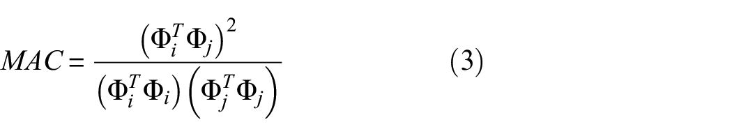
where
In equation (3), the element values in the MAC matrix range between 0 and 1, where 0 indicates that little or no correlation exists between the off-diagonal element

where
FIM
FIM,65,66 which is related to the information stored in the measured response, results from minimizing the covariance matrix of the estimated error for an efficient unbiased estimator from the statistics perspective. FIM can be obtained using equations (5) and (6)

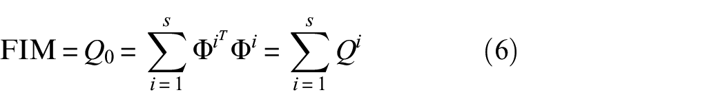
where
The procedure of using FIM for optimizing sensor placement is to unselect candidate sensor locations to maximize FIM. Three variants of FIM are usually used, the determinate, the trace, and the minimum singular value, to be maximized in order to increase the information or decrease estimate uncertainties. Although these are three different variants of FIM, different sensor placement approaches using these variants as the evaluation criteria should yield similar results.67,68
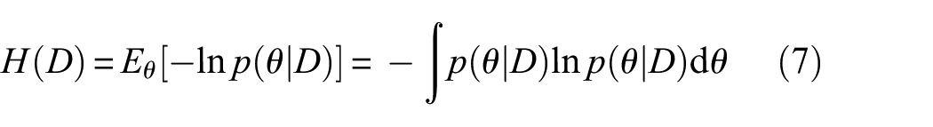
IE
In order to accurately estimate the model parameters for structural damage detection, the quality of the collected information from the installed sensors requires to be guaranteed. Since IE
69
is efficient to quantify the parameter uncertainties, Papadimitriou et al.
57
used IE as a measure of minimizing the uncertainty in model parameter estimate when optimizing the sensor placement.
70
In the IE-based OSP studies, the model updating was usually realized based on a Bayesian statistical method. A probability density function (PDF)
where

where
EI
EI, as one of the most significant and widely used criteria in large structural dynamic testing and model updating, was proposed by Kammer. 65 An efficient unbiased estimator, the covariance matrix of the estimated error can be obtained using equation (9)
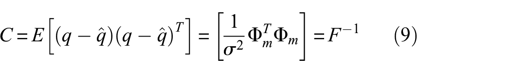
where C is the covariance matrix, and F is the FIM;
According to the statistics theory, 71 the effectiveness of the estimated parameters can be improved by maximizing the information in Fisher’s sense. To achieve this, the EI indicator is calculated using

where
EFI-DPR
The EI provides an estimation of the linear independence of target modes and is efficient in terms of computation. However, sensor positions that have low energy can be chosen, which results in a reduction of the signal-to-noise ratio that makes mode shape identification difficult. To overcome this drawback, the EFI-DPR (driving-point residue) method, 43 which weights the EI indices with the associated driving-point residue (DPR), 72 was used. DPR can be calculated as follows

where ⊗ is a term-by-term matrix multiplication.

where ⊗ denotes the same item to equation (11) and
Energy-based criteria
There are also some other evaluation criteria based on the energy for the sensor configuration. One commonly used criterion is the modal strain energy (MSE),33,37,74 which helps to select the sensor positions with possible large amplitudes. It can be used to increase the signal-to-noise ratio that is important in real situations. The MSE can be calculated using equation (13)
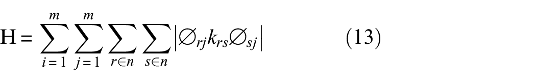
where the mode shape matrix is
The kinetic energy (KE) is another commonly used criterion.43,60 It aims at obtaining a reduced configuration of sensor placements that maximizes the measure of the KE of the structure. Besides, energy efficiency had also been commonly used as the objective to determine sensor configuration on large and complex civil structures.25,30,75–77
Optimization methodologies
Several optimization methodologies are available for sensor configuration determination. As mentioned in section “Problem formulation,” OSP mainly aims at assigning m sensors to n candidate positions (i.e. DOFs) on the target structures (e.g. buildings, bridges, and towers), which is usually treated as the combinational optimization problem. Therefore, evolutionary optimization methodologies that have the advantages of solving NP-hard problems can well address OSP problems. Besides, sequential sensor placement (SSP) algorithms, deterministic optimization methodologies, probability-based methodologies, and other optimization methodologies are also available for OSP problems. Details of each category of optimization methodologies are introduced in this section.
Evolutionary optimization methodologies
Evolutionary algorithms, which are based on a powerful principle of evolution (i.e. the survival of the fittest), constitute a critical category of heuristic search. 78 Evolutionary algorithms have been commonly utilized in science and engineering for addressing complex problems, such as the NP-hard problem of sensor placement. 79 Figure 2 illustrates the procedures in evolutionary algorithms. The evolutionary algorithms usually start from initializing a population with a certain number (i.e. population size) of candidate solutions. Then, the population is updated using evolutionary strategies (e.g. the genetic operators such as crossover and mutation in the genetic algorithm, position and velocity update mechanism for particles in particle swarm optimization (PSO)) based on the fitness function (i.e. the introduced evaluation criteria of sensor placement as mentioned in section “Evaluation criteria”). Finally, the evolution of population ends until a certain termination criterion is met. The best solution in the latest population is used as the optimal solution.
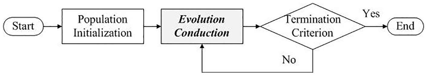
Illustration of procedures in evolutionary algorithms.
There are quite a few commonly used evolutionary algorithms, including genetic algorithm, PSO, monkey algorithm, firefly algorithm, simulated annealing algorithm, and ant colony optimization. The evolutionary algorithms and their improved variants for OSP are summarized in Table 1. Details of each evolutionary algorithm are introduced in the following sections.
Evolutionary methodologies used in sensor placement optimization.
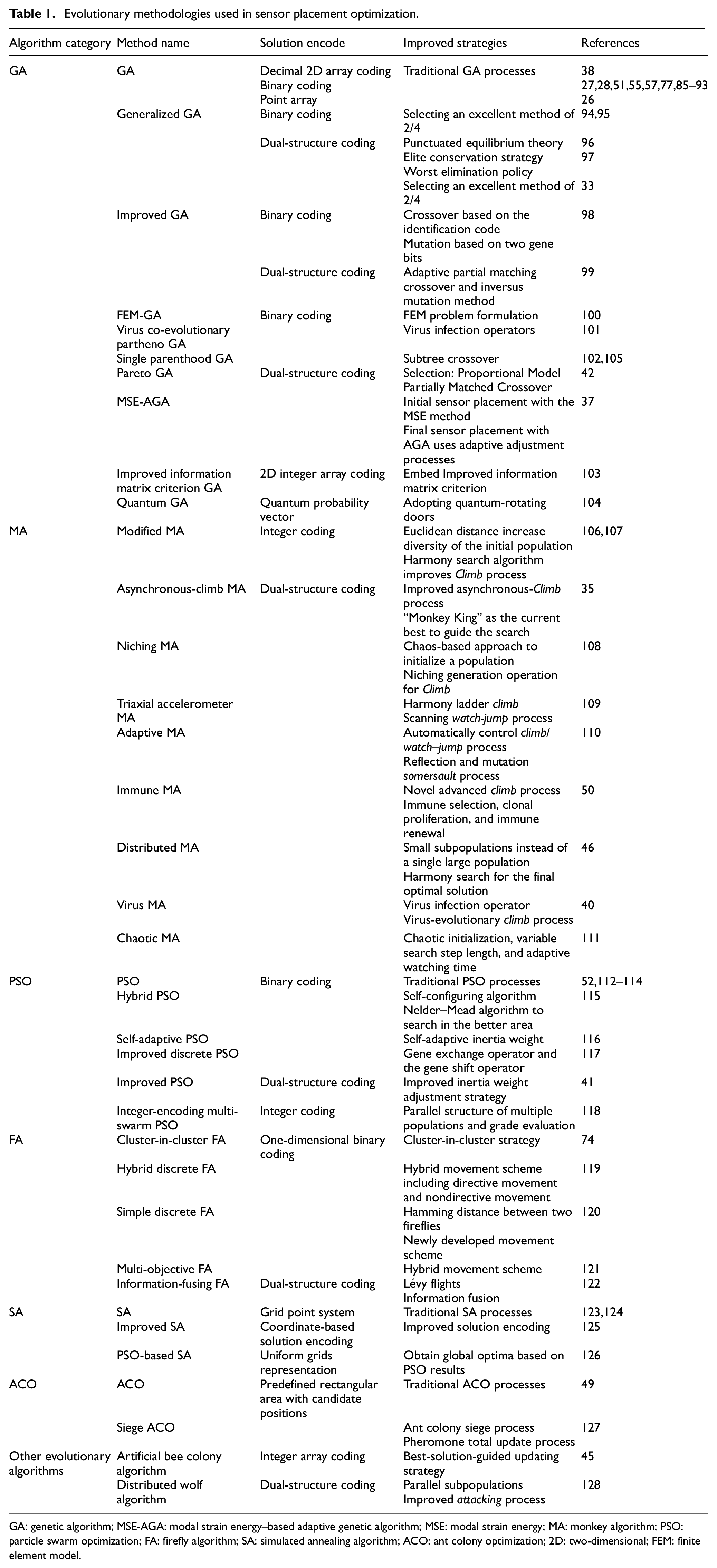
GA: genetic algorithm; MSE-AGA: modal strain energy–based adaptive genetic algorithm; MSE: modal strain energy; MA: monkey algorithm; PSO: particle swarm optimization; FA: firefly algorithm; SA: simulated annealing algorithm; ACO: ant colony optimization; 2D: two-dimensional; FEM: finite element model.
Genetic algorithm
Among the evolutionary algorithms, genetic algorithm (GA) is the most widely applied in engineering problems. 80 GA was first introduced in 197581,82 which was inspired by the mechanism of natural evolution. 83 The algorithm usually starts from initializing a population with a certain number of solutions (i.e. encoded chromosomes), and then the evolution conducts based on genetic operators, including replication, crossover, and mutation. The fitness function is used to evaluate newly generated solutions during iteration until a certain termination condition is reached. More details of the original GA process can be referred to Davis. 84 As mentioned in section “Problem formulation,” the OSP problem is usually considered as an NP-hard problem. GA is one of the commonly used heuristics methodologies to solve NP-hard problems. Both original GA26–28,38,51,55,57,77,85–93 and improved GA33,37,42,94–104 had been used in OSP problems.
Solution coding of GA
Chromosome coding is an important component of GA. Since the widely used objective is to place

where
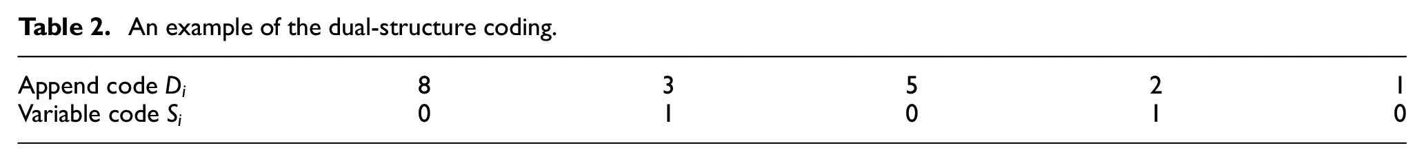
In addition to the binary coding method, dual-structure coding that contains two rows as presented in Table 2 has been used in GA-based OSP studies.96,97 The first row
An example of the dual-structure coding.
Besides, other solution representations have been proposed in previous GA-based OSP studies. For example, Liu et al. 38 developed a decimal two-dimensional (2D) array coding method that was similar to the dual-structure coding method. Huang et al. 26 proposed a point array coding method that included both sensor locations and sensor type information. Zhan et al. 103 presented a 2D integer array coding method. Zhu et al. 104 used quantum probability vector to encode the solution, where the quantum information was encoded using pairs of complicated numbers.
Improved GA
To obtain a better evolution performance in OSP problems, such as more stable iteration and efficient convergence, GA has been improved using different strategies. Generalized GA,
129
which utilizes the selecting method of excellent of 2/4 when formulating a new generation, was used in previous works.33,94,95 Selecting the excellent from both parent and offspring generations based on their fitness ensures a stable iteration. Besides, Yi et al.
96
adopted a “group in group” scheme to generate a leading population by selecting a small population with
Guo et al.
98
developed a new crossover and two-gene-bite mutation to generate new binary string named identification code to guarantee that the new offspring does not violate the constraints. Shan et al.
99
used the adaptive GA approach
130
to improve the capability of global search and change the probabilities of crossover
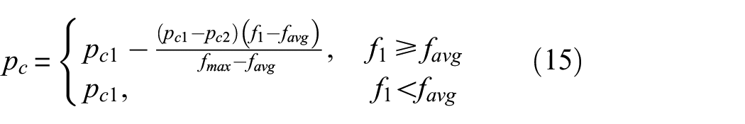
where
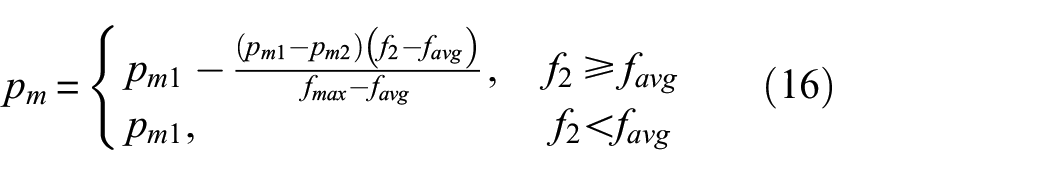
Kang et al. 101 involved parthenogenesis 131 in their proposed partheno genetic algorithm (PGA), which contained three basic partheno-genetic operators, namely, swap, reverse, and insert.132–134 In order to improve the operation, virus infection operators135–138 were also introduced in the PGA. Zhang et al. 42 adopted a proportional selection model to guarantee the quality of the population, and the partially matched crossover was implemented to improve the evolution performance. In addition, Zhan et al. 103 embedded an improved information matrix into GA for sensor placement design. Zhu et al. 104 adopted the quantum theory to improve GA performance, where chromosomes are represented with quantum probability vectors, and quantum-rotating doors were used to update and optimize the population by globally searching for an optimal solution. Vosoughifar et al. 100 developed a hybrid FE-approach to select the best sensor position for a cold-formed steel structure based on the blast loading response of the system. He et al. 37 proposed a hybrid optimization approach named modal strain energy–based adaptive genetic algorithm (MSE-AGA) to address the OSP problems, where MSE methodology was used to conduct initial sensor placement to determine the candidate sensor locations, and AGA was used to determine the final sensor placement.
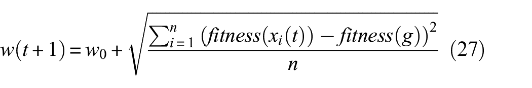
Monkey algorithm
Monkey algorithm (MA) is originally designed by Zhao and Tang 139 to solve the optimization of multivariate systems. MA simulates the mountain-climbing processes of monkeys to find the highest mountaintop, which was used as the optimal value of the objective function. 139 The mountain-climbing processes are used to conduct the evolution or iteration during optimization. The evolution processes are usually decomposed into four main steps: climb, watch, jump, and somersault. A monkey (i.e. one potential solution) climbs from the current position (i.e. initial position) to the top of the mountain where it locates (i.e. usually treat as local optimum), then it watches around to find out whether any neighbor mountaintop is higher than the current one. If yes, it jumps to the higher mountaintop. In order to find a much higher mountaintop, a monkey somersaults to a total new mountain area (i.e. new search domain). The detailed mathematical representations of MA solution and the four mountain-climbing steps can be referred to Zhao and Tang. 139
Solution coding of MA
Since MA was first applied in sensor placement problem Yi et al.,
106
quite a few studies explored original MA and its improved versions for OSP. As an emerging evolutionary algorithm, solution representation or encoding usually requires to be determined before evolution implementation. MA is originally designed to solve optimization problems with continuous variable.
139
However, OSP aims at determining discrete sensor locations, which is usually treated as an optimization problem with discrete variables as mentioned in section “Problem formulation.” Instead of the traditional one-dimensional binary coding, which requires increased string length and computational time when sensor number increases, Yi et al.
107
proposed an integer coding. For one monkey (i.e. one potential solution), its location is defined as a vector
In addition to the integer-coding method, a developed dual-structure coding method is more common in the MA-based OSP problem.35,40,46,50,108–111 In this dual-structure coding method, an ordered pair
Suppose there be
For ith monkey in the initial population, its solution of the proposed optimization problem is denoted as
where
When using equation (17), a threshold
Improved MA
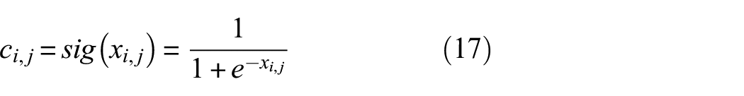
To improve the evolution performance, several strategies are proposed to improve MA in different perspectives. Since MA is swarm intelligent algorithm, which evolves based on population, increasing the quality and diversity of the population can avoid generating similar monkey positions and improve the evolution. For example, Yi et al. 107 adopted Euclidean distance that could increase the diversity of the positions of monkeys, reducing the possibility of being trapped in local optima. Euclidean distance (Ed) is defined as
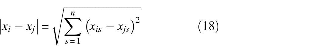
where

where
Determine the initial chaos variable
Generate the chaos variable
Obtain the jth variable in the position vector of the ith monkey using equation (20)

where
4. Repeat Steps 1–3, until
The chaotic-based approach was applied Zhang et al. 111 Yi et al. 46 also introduced a distribution mode of multiple monkey populations, where small subpopulations were used instead of a single large population. Original MA is executed on each subpopulation separately. Then, the harmony search algorithm (HSA), 141 which is integrated with the dual-structure coding method, is used to obtain the final optimal solution.
In addition to the population, the performance of MA is also improved by improving the evolution process. The climb is the main process to change the positions of monkeys from the initial positions to the new ones with the improved fitness values. Therefore, to improve the climbing process results in a better evolution, Yi et al.
107
used the stochastic perturbation mechanism of HSA after a large-step climb process to keep the diversity of the monkeys. The pitch adjusting rate in the HSA is adapted to the new components

where
Yi et al. 35 developed an asynchronous-climb process, which is motivated by the simulation of the social behavior of monkeys. In the asynchronous-climb process, monkeys move around the search space and exchange information with others using equation (22)
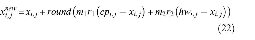
where


where
In addition, Yi et al. 108 significantly modified the climbing process using the niching techniques. Jia et al. 109 proposed a harmony ladder climb process, where stochastic perturbation mechanism of the HSA was used to avoid the problem of premature convergence; Yi et al. 110 designed a novel adaptive scheme to automatically control the implementation of climb process. Yi et al. 50 also improved the climbing process by dividing the entire climb process into initial and advanced climb process. Yi et al. 40 incorporate virus theory 142 into the climbing process to search the solution in a better local area.
Other processes of MA, such as watch and jump, were also improved. For example, in the original MA, eyesight constant is used to watch around for a higher mountaintop (i.e. a better solution). Either too large or too small values can lead to a miss of better solution nearby. Therefore, Jia et al. 109 proposed a scanning watch-jump process that reduced the probability of missing a nearby higher mountain. Besides, Yi et al. 110 developed a novel adaptive scheme to control the implementation of the watch-jump process automatically.
PSO
PSO algorithm, which imitates the social behavior of the flocking of birds, was originally introduced in 1995 by Eberhart and Kennedy. 143 In PSO, each solution is a point in the D-dimensional search domain that can be treated as a bird or a particle. All particles, which have fitness and velocities, fly through the search space by learning from the best experiences among all the particles. The velocity and position of each particle are updated using equations (25) and (26) 143


where
Several OSP studies have utilized traditional PSO processes to obtain the best locations of sensors in SHM systems for different large structures, such as long-span cable-stayed bridges,112,113 truss structure, 114 and an aluminum plate. 52 As for the coding of the PSO solution, two commonly used methodologies, binary and dual-structure coding methods, are the same as introduced in GA and MA sections. In addition to applying the traditional PSO process for OSP problems, researchers also tried to improve its performance during sensor placement optimization.
Improved PSO
Since the introduction of PSO in 1995, PSO obtains increasing attention for the past decades. Quite a few researchers have attempted to improve its performance with different efforts and to develop several interesting variants.145–148 In the PSO-based OSP studies, various strategies are proposed by different researchers to improve the performance of PSO when optimizing the sensor locations. For example, Rao and Anandakumar
115
tuned the behavior of the PSO algorithm qualitatively and quantitatively by adjusting the PSO parameters dynamically, which achieved a large diversity of generation. In addition, the Nelder–Mead algorithm,
149
which was used to conduct a local search, was used to obtain a better local area. According to equation (25),
where
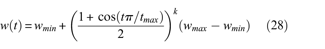
where
In addition, to avoid PSO being trapped in a local extreme value and the phenomenon of prematurity, Lian et al. 117 proposed a hybrid approach of clonal selection and discrete PSO. Clonal selection approach (CSA) is a clonal selection theory-based immune optimization algorithm, which guarantees the diversity of antibodies in the system. Besides, He et al. 118 proposed a parallel structure-based integer-coding multi-swarm particle swarm optimization (IMPSO) approach, which simulated biogenic accumulation forms, using grade evaluation to guarantee the diversity of the population, avoiding being trapped in the local optimum.
Firefly algorithm
Firefly algorithm (FA), which is a newly developed swarm intelligence algorithm,150,151 mimics the social behaviors of fireflies, such as communication, search for food, and mates finding. FA optimization process is conducted in the way that a firefly (i.e. a solution) with a low light intensity (i.e. low fitness) will be attracted and moved to a firefly with a high light intensity (i.e. high fitness). Therefore, to model this process with mathematical representation, three hypotheses are applied: (1) Attractive action among fireflies is inspired by light intensity; (2) the firefly light intensity that is based on the location of a firefly is proportional to the objective function; and (3) the light intensity weakens when the distance increases. Then, the movement of firefly
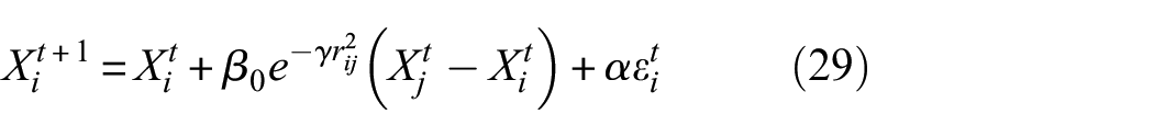
where
Like other swarm-based intelligence algorithms, FA encodes the solution using one-dimensional binary coding and dual-structure coding methodologies as mentioned previously. More details of both coding methods can be found in the sections of GA, MA, and PSO.
Improved FA
Since the original FA is proposed to solve continuous variable problems, FA requires being modified and improved to fit the OSP problem that is usually treated as a knapsack problem, selecting specified DOFs for sensor placement to effectively describe the structural performance. There are several studies aiming at improving FA for OSP problems. For example, in order to improve the speed of convergence and avoid trapping in a local extreme value, Zhou et al.
74
introduced the cluster-in-cluster strategy, which divided the fireflies into several clusters. The firefly cluster is usually formulated based on the Hamming
152
distances. The firefly of the highest light intensity of each cluster is selected as the cluster-head. Fireflies only move with their own cluster to shorten the movement time. Besides, the Hamming distance was also applied by Zhou et al.
119
in order to describe the distance among fireflies. They proposed the hybrid discrete firefly algorithm (HDFA), which used a hybrid movement scheme, including directive and nondirective movements, to enhance the robustness of the HDFA to obtain the best sensor configuration. Zhou et al.
120
also used the Hamming distance to represent the distances among fireflies, and they developed a movement scheme that involves stochastic searching, where the distance

where
Obtain the difference between the

2. Select
3. The string of

where
In addition, Hao and Zhang 121 proposed a multi-objective FA that also used a hybrid movement scheme to optimize wireless sensor placement trade-off energy efficiency and modal independency while guaranteeing the connectivity of the sensor network. Zhou et al. 122 utilized Lévy flights,153–155 which were the typical flight behaviors among insects and animals, to drive fireflies flying to fireflies with a higher light intensity, where the computational performance was improved. Besides, information fusion was used to improve the original FA by speeding up the convergence and avoid being trapped in a local optimum.
Simulated annealing algorithm
Simulated annealing (SA) algorithm, which is based on the studies of Metropolis et al. 156 and Kirkpatrick et al., 157 is an optimization process simulates thermodynamic physics process of metal cool and anneal. 158 The actual implementation for OSP problems is defined by the fitness function, perturbation operator, parameter setting, and constraints. 159 The annealing process (i.e. iteration) is driven by perturbation operators. During the SA iteration, every variable is selected for perturbation randomly. Then, the operator uses direction cosines for each variable to obtain a random direction. Constraints guarantees that the iteration is conducted within the search domain until an optimal solution is reached. Chattopadhyay and Seeley 160 used SA for both discrete and continuous issues when designing intelligent structures, and SA outperforms previous nonlinear programming approach in computational performance. Therefore, SA can also be implemented to solve the OSP problem, which is usually treated as the combinational problem. Chiu and Lin 123 used SA to address the OSP problem for target location considering limited cost and complete coverage. Gou and Cui 124 proposed a mathematical model to minimize the total energy of sensor placement on a simple beam based on both GA and SA.
Improved SA
In addition to implementing traditional SA, some studies attempted to improve SA to better address the OSP problem. For example, Tong et al. 125 developed a coordinate-based solution encoding (CSA) to involve more spatial information that was usually limited in the traditional one-dimensional coding method. CSA allows conducting a search in all directions simultaneously, resulting in a better chance to avoid being trapped by a local extreme value. Wang et al. 126 integrated PSO with SA to improve the chance to obtain the optimal configuration of the WSN. PSO was used to get several local best locations of particles during the iteration; then SA was applied to these local optimal solutions to obtain the best global solution. Besides, SA is integrated with the adaptive mechanism in order to guarantee the quality of the solution and to improve the convergence speed of GA. 161
Ant colony optimization
The ant colony optimization (ACO) algorithm utilizes an artificial ant colony, where all ants cooperate to search (i.e. iteration) and reinforce pathways (i.e. solutions) to obtain the shortest pathway (i.e. optimal solution). 162 In order to use ACO for OSP problems, the modification is required as ACO usually works on a travel salesman problem. 163 Fidanova et al. 49 used the MAX–MIN ant system 164 to deploy the WSN that can fully cover the sensor field with the minimum number of sensors and maintain the network connectivity. In addition, Feng et al. 127 improved ACO by proposing an ant colony siege process to improve the efficiency of the sensor configuration. Since pheromone updating, which is the basic updating method used to find better pathways in original ACO, does not work in OSP problem, a novel approach named pheromone total update process was presented. More details of this novel approach can be referred to Feng et al. 127
Other evolutionary algorithms
In addition to the commonly used algorithms as mentioned above, other evolutionary algorithms have also been proposed for OSP problems. For example, Sun and Büyüköztürk 45 used the artificial bee colony (ABC) algorithm, which is inspired by imitating the foraging behavior of honey bees, to solve the OSP problem. A new solution updating approach that transforms continuous solution into an integer version was proposed in the developed discrete ABC approach. Yi et al. 128 proposed a distributed wolf algorithm (DWA), which was inspired by wolf behaviors for food hunting, for OSP problems with faster convergence and a higher capability of searching.
SSP algorithm
In addition to evolutionary algorithms, another efficient heuristic algorithm named SSP algorithm 86 has also been proposed for OSP problems. SSP is usually divided into two types, namely forward sequential sensor placement (FSSP) and backward sequential sensor placement (BSSP). As for FSSP, the positions of all the sensors required to be placed are sequentially computed by placing one sensor each time on the structure at a position, which reduces the maximum off-diagonal element of MAC most165,166 or leads to the smallest increase in IE.70,167–169 Usually, the position of the first sensor is selected as the one with the optimum value of the criteria used for sensor configuration evaluation for the one-sensor scenario. Then, the position of the first sensor is fixed. The position of the second sensor will be selected as one that also leads to the optimum value of the criteria for the two-sensor scenario. Such sensor placement continues until all sensors have been placed on the target structure. The SSP algorithm can also be used inversely. Starting with all sensors placed at all DOFs of the target structure and successively removing one sensor each time from the position. This algorithm is termed as BSSP.
Deterministic optimization methodologies
Several constrained (linear and nonlinear programming) 170 and unconstrained (Newton methods) 171 deterministic optimization methods have been proposed for OSP problems. Usually, simple deterministic approaches are sufficient to conduct a local search, and the constrained optimization owns a high degree of complexity. 172 For SHM with simple and regular shapes such as beam and plates, optimal sensor configuration can be determined directly using constrained deterministic techniques like recursive quadratic programming approach,173,174 as their mode frequencies and shapes can be represented directly with an analytical expression. OSP problems are usually defined as integer programming problems that are more complicated and costly to be addressed, compared to continuous optimization problems. Therefore, discrete variables are converted as continuous variables and then addressed with deterministic optimization techniques. For example, Sepulveda et al. 175 proposed a control-augmented structural synthesis approach, which treats the placement of actuators and sensors as mixed 0-1 continuous variable design problem. 176 Sunar and Rao 177 well addressed the thermopiezoelectric sensor placement on the cantilever beam-like structures based on quasistatic thermopiezoeletricity equations.
Probability-based methodologies
Some studies also used Bayesian theory to determine the sensor configuration. For example, Capellari et al. 178 developed an OSP approach by integrating Bayesian inference with a stochastic search algorithm. Flynn and Todd 53 proposed a Bayesian probabilistic framework to place active sensors for crack detection on unknown positions. Yuen et al. 179 presented an IE-based framework to select optimal sensor configuration using the Bayesian statistical method. Besides, Azarbayejani et al. 180 developed a probabilistic approach, which used the weights of a neural network that was trained based on simulations to produce a normalized probability distribution function to determine the optimal sensor configuration.
Other optimization methodologies
In addition to the aforementioned optimization methodologies, various researchers also used different techniques to determine the sensor configuration. For example, Guratzsch 181 used Snobfit, 182 which was an optimization strategy designed for bound-constrained optimization of noisy objective functions, to determine the sensor layout.183,184 Using Snobfit, no candidate sensor positions require being previously determined. Kalman filter algorithm, 185 which estimates the state vector and its corresponding error variances, is integrated with sequential placement strategies to address OSP problems.39,186 Besides, many other methodologies, such as backup sensor-based fault-tolerance SHM method, 30 energy-efficient sensor deployment, 76 frequency domain–based OSP technique, 187 mixed variable pattern search algorithm, 188 Gram–Schmidt orthogonalization procedure, 72 three-phase sensor placement approach, 29 e-Estimator algorithm, 75 and wave propagation-based local interaction simulation approach, 189 are also available for OSP. More development details of these methodologies can be referred to the associated studies.
Besides, there is also a trend to use machine learning (ML), which automatically improves or learns from the study or experience, and acts without being explicitly programmed,190,191 to optimize sensor placement. ML is a method of data analysis that automates analytical model building. To a certain degree, ML with its iterative feature helps improve the efficiency of the formulation and training of the sensor placement optimization model. According to the existing studies of applying ML algorithms for OSP problems, a supervised learning algorithm takes the instantaneous signals (pressure or wall shear stress) from the civil structures as input variables and function characterizing the instantaneous flow state as the output and trains a ML model to generate predictions for the response to new input data. The optimal sensors are usually determined as the input signals (from their corresponding locations) with the highest relevance to the trained model. For example, Semaan 192 introduced a new ML-based approach, which first formulates ML models based on a range of input sensors to predict a response function. Then, the optimal sensor positions are determined as the most relevant features according to variable importance ranking. Amin and Riza 193 presented an ML-enhanced optical distance sensor, where a regularized polynomial regression–based supervised ML algorithm is used to increase the accuracy of the sensor. Yoganathan et al. 194 proposed a novel data-driven approach that integrated clustering algorithms, information loss approach, and Pareto principle to optimize the sensor placement in an office building. In addition, Praveen Kumar et al. 195 reviewed various ML-based algorithms for WSNs. The advantages and drawbacks of these algorithms were discussed. Compared to the existing approach, ML-based solutions for OSP usually have the advantages of simplicity, adaptivity, and low computational cost. 192
Comparison of the main computational methodologies for OSP
After reviewing the summarized computational methodologies for OSP, it can be concluded that quite a few computational methodologies can be applied for sensor configuration determination in different structures. Each methodology has its own advantages or disadvantages when being used to solve the OSP problem of SHM. As the most widely used methodologies, evolutionary algorithms show their advantages on sensor placement compared to traditional optimization approaches as the OSP is usually treated as the combinational problem (i.e. NP-hard problem). Although different algorithms with their variants show different computational performance when addressing OSP, how to improve the original algorithm with different improving strategies is shared by all the evolutionary algorithms as presented in Table 1, including new solution coding system, new operators, improved movement scheme, and iteration strategies. In addition to introducing the improved algorithms, the advantages and disadvantages of mainly review computational methodologies as well as the suitable applications for each of them have been summarized in Table 3.
Comparison of OSP computational methodologies.
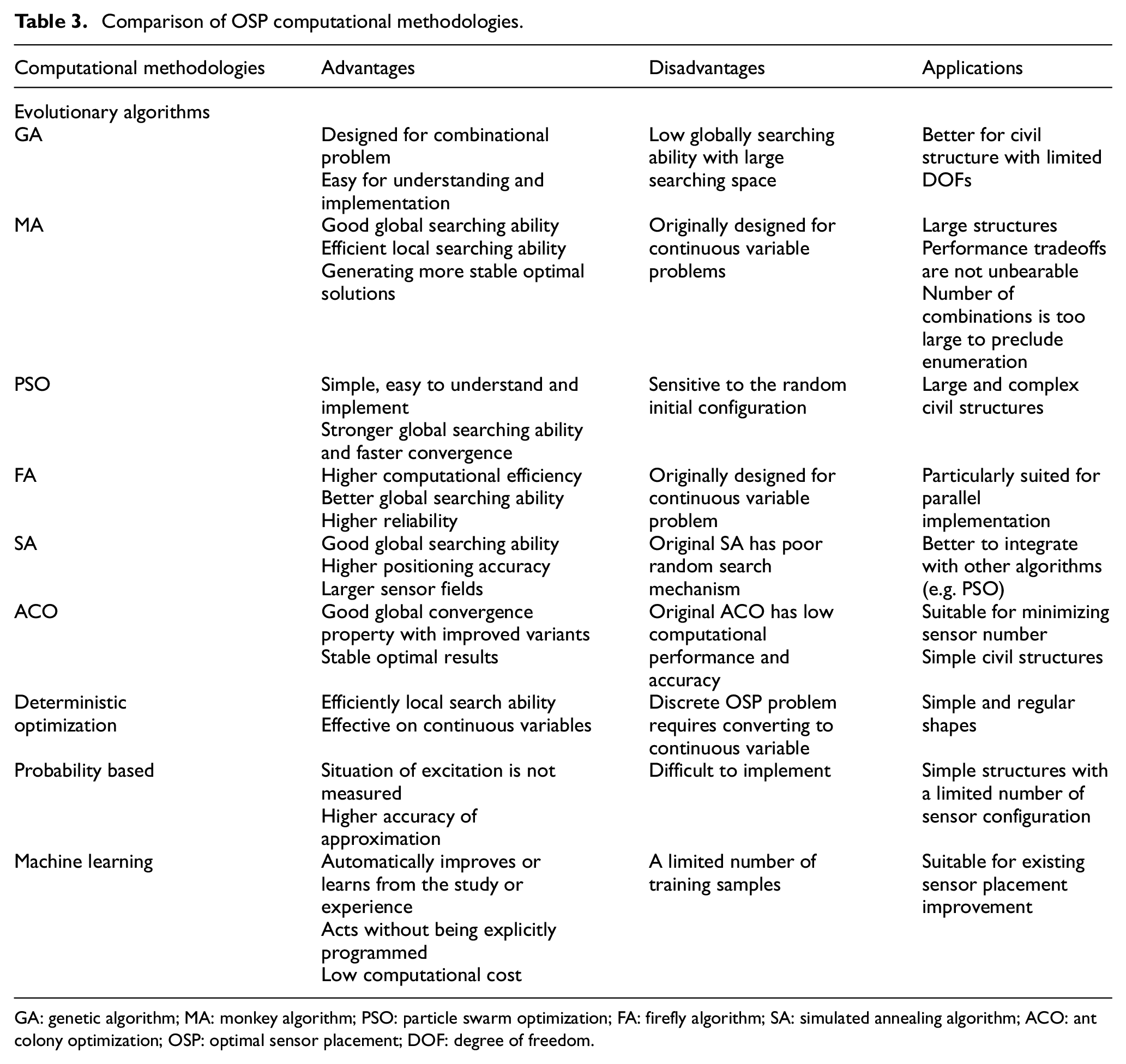
GA: genetic algorithm; MA: monkey algorithm; PSO: particle swarm optimization; FA: firefly algorithm; SA: simulated annealing algorithm; ACO: ant colony optimization; OSP: optimal sensor placement; DOF: degree of freedom.
Specific SHM applications
In addition to comparing different computational methodologies utilized in OSP of SHM, the studies of specific applications, including the most widely used vibration-based and ultrasonic-based damage detection methods in SHM, had also been explored. Vibration-based damage detection approaches monitor changes in natural frequencies, vibration modes, and related derivatives. 90 Besides, as most of the structural elements of civil infrastructures are natural waveguides, ultrasonic-based damage detection methods are also utilized in SHM. 54 For these two specific damage detection methodologies in SHM, evolutionary algorithms are mainly used to obtain the optimal sensor configuration. For example, Rao and Anandakumar 115 proposed a PSO-based positioning algorithm for sensor in large-scale structures, where the best identification of frequencies and modals was achieved. Gomes et al. 90 employed GA to locate the best sensor configuration to cover a specific number of low-frequency modes for laminated composite plates under vibration. As for ultrasonic-based SHM application, Gao and Rose 54 used covariance matrix adaptation evolutionary strategy (CMAES) to determine the sensor number and sensor distribution in SHM. Guo et al. 98 adopted GA to search for the optimal locations of sensors. According to the mentioned studies of specific SHM applications, it can be found that evolutionary algorithms are more commonly employed to obtain the optimal sensor configuration.
Conclusion
This study provides a comprehensive review of the computational methodologies for OSP in SHM. First, the problem formulation of OSP is presented. To determine the sensor configuration for various types of structures (e.g. buildings, bridges, and towers), associated 3D FE models consisting of a certain number of DOFs are usually constructed for the numerical experiment as physically testing different sensor configurations are impossible. The OSP is treated as a combinational problem, which aims at assigning sensors to candidate DOFs of the target FE model. Commonly used criteria, including MAC, FIM, IE, EI, and EFI-DPR, are summarized and introduced in detail. Then, optimization methodologies for OSP are introduced.
This study covers most of the existing optimization methodologies, including evolutionary algorithms, SSP methodologies, deterministic optimization, and probability-based methodologies. Since evolutionary algorithms outperform other methods when addressing combinational methodologies, the most widely used evolutionary algorithms (e.g. GA, MA, PSO, FA, SA, and ACO) and their improved variants are summarized in detail. ML algorithms are also identified as the emerging techniques for OSP considering their advantages over traditional approaches. Besides, the advantages and disadvantages of the main computational methodologies as well as the suitable applications for each of them are also summarized and compared. Finally, the study briefly discussed the suitability of computational methods for specific SHM applications, where evolutionary algorithms are more commonly utilized. With the reviewed problem formulation, commonly used optimization methodologies, and the summarized pros and cons of each methodology, this study provides an effective reference for OSP in SHM. Researchers are expected to not only better understand the OSP problem but also conduct the OSP study in a more efficient manner.
Footnotes
Declaration of conflicting interests
The author(s) declared no potential conflicts of interest with respect to the research, authorship, and/or publication of this article.
Funding
The author(s) disclosed receipt of the following financial support for the research, authorship, and/or publication of this article: This study was financially supported by the Start-Up Grant at Nanyang Technological University, Singapore (No. M4082160.030), the Ministry of Education Tier 1 Grant (No. M4011971.030), and Start-Up Grant at Shenzhen University, China (No. 2019092).