
Abstract
Extracting bearing degradation curves with good smoothness and monotonicity as a health indicator lays a solid foundation for predicting the bearing’s remaining useful life. Traditional bearing health indicator construction methods generally have the following problems: (1) they require manual experience, such as manual labeling of data is burdensome when the amount of collected data is large, for feature extraction, selection, and fusion with other indicators and models because the methods rely on substantial expert experience and signal-processing technology; (2) deep belief networks in deep learning require engineering experts with rich experience to label the data, and because the degradation state of a bearing is constantly changing, it is difficult to rely on manual experience to distinguish and label it accurately; (3) owing to the noise in the data collected during the study, the extracted health indicator curve shows obvious oscillation and poor smoothness. In response to the above problems, this study proposes a model based on an unsupervised deep belief network and a new sigmoid zero local minimum point to eliminate health indicator curve oscillation and improve monotonicity. The main idea is that a deep belief network without a label output layer is used to extract the preliminary health indicator curve directly from the original signal, whereas the sigmoid zero local minimum point uses the average value based on a sigmoid function to reduce the weight of the current health indicator value to eliminate concussion, and then it uses the zero and local minimum points to further improve the monotonicity of the extracted health indicator without parameters. Finally, the superiority of the model proposed in this study (deep belief network–sigmoid zero local minimum point) is verified through a comparison of multiple bearing datasets and other models.
Keywords
Introduction
Rolling bearings are one of the most commonly used and most vulnerable mechanical parts in industry. Ensuring their reliable operating condition is of great significance to system safety and economic costs.1–3 Rolling bearings gradually lose their reliability over time. Constructing a health indicator (HI) that reflects the degradation of bearing performance is an important way to achieve a quantitative assessment of bearing health. In addition, extracting HI curves with good smoothness and monotonicity lays a solid foundation for predicting the remaining useful life of the bearing.
Common methods for extracting HIs include a single time–frequency domain indicator, the fusion of different time–frequency domain indicators, multiple entropy models, and a combination of signal decomposition models for HI extraction. Lei et al. 4 used root mean square (RMS) to extract HI, as did Shen et al. 5 Kosasih et al. 6 used kurtosis to extract HI. Tse and Wang 7 used various time–frequency domain indicators to generate HI. Yan and colleagues8,9 used approximate entropy (AE) and permutation entropy (PE) to extract HI and obtain good experimental results. To consider vibration signals with nonlinear characteristics, Rai and Upadhyay 10 used the empirical mode decomposition (EMD) to decompose the original signal adaptively into a series of intrinsic mode functions (IMFs), and then utilized singular-value decomposition (SVD) to extract degenerate feature vectors, and finally used K-means and K-medoids clustering methods to construct the final HI. However, these proposed models pose the following problems:
These models require extensive manual experience to select appropriate time–frequency domain indicators to extract HI. It is difficult to adapt the time–frequency domain indicators to the new system and extract useful HI when the industrial system changes.
The above models require a complex operation that combines multiple models. It is necessary to select a suitable combination of time–frequency domain indicators and models to achieve useful HI indicators. For example, the EMD–SVD–K-means/K-medoids in the study by Rai and Upadhyay 10 requires a combination of three models to extract the HI curve. In addition, principal component analysis is used to eliminate feature redundancy and extract HI when the extracted bearing degradation dimension is high. 7
The deep belief network (DBN) is one of the commonly used deep-learning models. 11 The hidden layer of a DBN uses a nonlinear function with adaptive features to extract the latent features of the data and can reconstruct the original data. Configuration of the number of nodes in the hidden layer is used to reduce the data dimensionality.12,13 Therefore, the DBN does not require experts who have extensive engineering experience with the system, and it can reduce complexity. Therefore, the DBN has been widely used in various engineering fields, such as speech recognition, 14 image processing,15–17 medical diagnosis, 18 and the fault diagnosis of bearings.19,20 Tamilsevlan et al. use DBNs for fault classification. 21 Zhao et al. 22 used the variation mode decomposition to decompose the vibration into IMFs, and then the Hilbert transform to extract the fault feature. Finally, the DBN was used to diagnose the fault. Guan et al. 23 presented a method based on variation mode decomposition, sample entropy, and the DBN for fault diagnosis. Wang et al. 24 developed a method based on spectral analysis with a sliding window to extract fault features, and then utilized the DBN for fault diagnosis. Shen et al. proposed an improved DBN, namely hierarchical adaptive DBN, for bearing fault diagnosis. The authors selected the frequency spectrum as the input for feature learning and then combined it with Nesterov momentum to adjust the learning rate in the DBN. 25
However, the above DBN and improved DBN models both require manual experience in labeling data. For example, the faulty bearing has an inner race fault and/or an outer race fault because of the great difference between these two faults, hence the fault label can be divided into several types, such as 1 and 2. However, the degradation state of the bearing vibration signal changes continually. It cannot be divided into several types. As in Figure 1(a), it is difficult to label the original data directly. Moreover, when the amount of data collected during a study is large, labeling data consumes considerable manpower and increases economic costs, and it is highly dependent on manual experience. To solve this problem, Xu and colleagues12,13 used the DBN without the output label layer to extract the fault characteristics of the bearing automatically, and combined the characteristics with the clustering model for fault classification. In that study, the authors used multiple hidden layers in the DBN to reconstruct the input data and extract the fault characteristics. Moreover, the multiple hidden layer structure was used for data dimensionality reduction, that is, the number of neuron nodes in the next hidden layer was half the number of nodes in the preceding hidden layer. Inspired by this idea, an unsupervised DBN based on a triangular structure was used to extract the HI of rolling bearings in this study. To the best of our knowledge, there are few reference reports that use an unsupervised DBN to extract bearing HI. Peng et al. 26 used an unsupervised DBN to extract the HI of the bearing and proposed an improved particle-filtering model to predict the remaining useful life of the bearing. In addition, the vibration amplitude of the signal reflects the health status of a bearing; for example, when the bearing wear is severe, the vibration amplitude is large. Therefore, we use a DBN without the output layer to directly extract the HI from the original vibration signal.
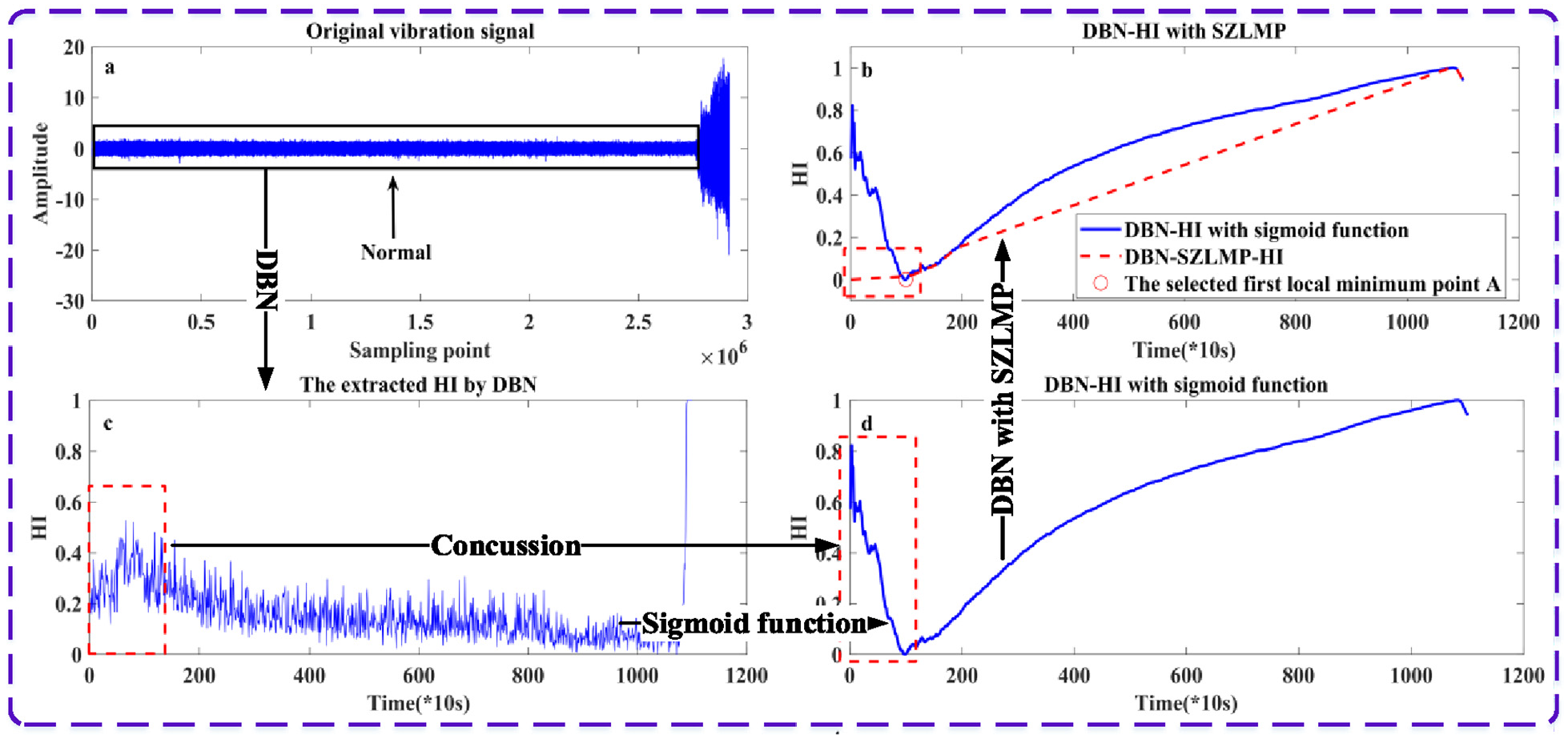
Original bearing vibration signal and the HI extracted through different models. (a) Original vibration signal; (b) the HI extracted through the DBN and SZLMP without an output layer; (c) the HI extracted through the DBN without an output layer; and (d) the HI extracted through the DBN and sigmoid function without an output layer.
However, the following problems remain:
The poor monotonicity of the HI curve leads to poor prediction results. As shown in Figure 1(c), the extracted HI curve in the black rectangular area extracted using a DBN maintains a steady trend, and there is no upward trend. Generally, the predicted value must exceed the threshold to determine the bearing health state and calculation of remaining useful life. Here the predicted remaining useful life is the difference between the length of time for the predicted value of HI to exceed the threshold and the length of time to train the data for the prediction model. However, the HI curve in Figure 1(c) remains stable for a long time, hence the predicted value does not easily exceed the threshold to render a prediction.
Due to the random noise in the vibration data collected during the actual project, the extracted HI curve oscillates and degrades the life prediction. As shown in Figure 1(c), the HI curve in the dashed area contains a slight oscillation. Because the bearing and the mechanical system are not fully adapted, there is a slight vibration in the signal. The life prediction generally uses the previous period of HI data. As shown in Figure 1(d), 200 pieces of HI data in the red rectangular area were used to train the prediction model, and all the remaining HI data were used to test the performance of the prediction model. However, there were oscillations in the first 200 HI values. For example, the trend of the HI curve decreases first and then rises, which results in poor prediction performance. The ideal pattern of the HI curve extracted by the signal amplitude is a steady increase with time growth.
To solve these problems, a new model, namely one with a sigmoid function with zero local minimum points (SZLMP), is proposed to eliminate the HI curve oscillation and improve its monotonicity. As shown in Figure 1(b), after the HI curve in the red rectangular area is replaced (see the red dotted line), the oscillation phenomenon disappears. The main idea of the SZLMP is first to calculate the average value of HI from the start to the current time, and then as the input of the sigmoid function. If the HI value at the current time has a significantly violent oscillation, SZLMP uses the average value to reduce the dependence and weight on the HI value at the current time and to reduce the oscillation. In addition, a monotonically increasing sigmoid function is used to enhance the monotonicity of the HI. In summary, this study proposes a model based on an unsupervised DBN and SZLMP. The DBN is used to extract the HI from the original vibration signal directly to reduce manual experience, such as labeling data. The SZLMP model is used to further improve the monotonicity of the extracted HI and eliminate the concussion at the same time. The main contributions of this study are as follows:
To reduce the dependence on manual experience, an unsupervised DBN model is used to extract the preliminary HI directly from the bearing’s original vibration signal without data labeling.
A new SZLMP model is proposed and used to improve the smoothness and monotonicity of the HI curve. In addition, there are no parameter settings in the SZLMP.
In order to verify the superiority of the proposed model (DBN–SZLMP), we compare it with other models, such as RMS, Kurtosis, AE, PE, various time–frequency indicators in the study by Tse and Wang, 7 EMD–SVD–K-means/K-medoids in the study by Rai and Upadhyay, 10 the unsupervised DBN and the stacked auto-encoder (SAE) with output label layer in the study by Xu et al. 27 Finally, several bearing datasets are used to verify the performance of our proposed model.
The rest of this article is organized as follows. The section “Procedure of the method presented” details the overall experimental process of the model proposed and uses the original data of the bearing to illustrate the detailed experimental steps. The basic theory and detailed calculation steps of the DBN and SZLMP are also presented. The section “Experimental setup” first introduces the experimental data information in detail, and then combines it with a bearing for experimental verification and comparison. Finally, the same model and parameters are used to verify other bearing datasets. The section “Conclusion” presents the conclusion.
Procedure of the method presented
There are four parts to the method presented: (1) data pretreatment; (2) HI extraction: first using the DBN without the output layer, and then the SZLMP is utilized to remove the concussion and improve the monotonicity of HI; and (3) experimental comparison and analysis. The detailed procedure of our proposed model is shown in Figure 2.
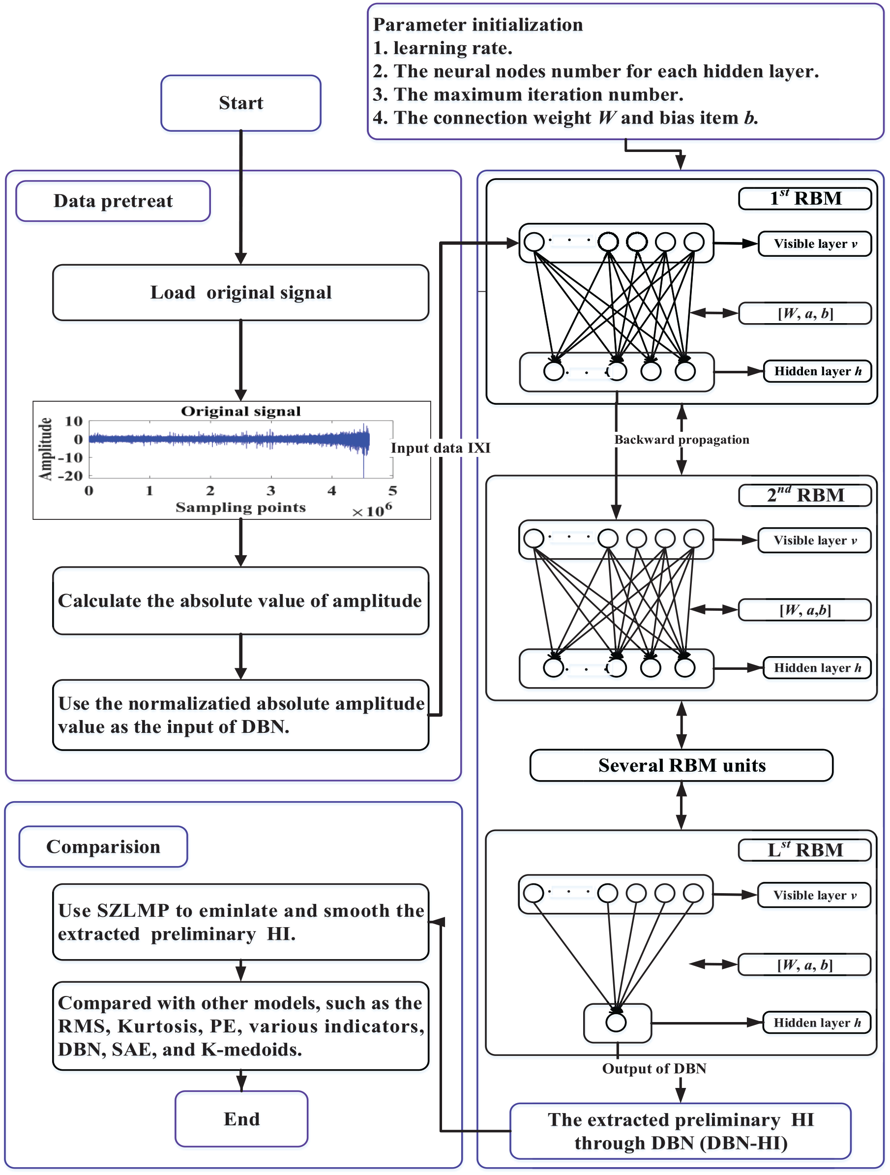
Flowchart of the proposed method. RBM: restricted Boltzmann machine in the DBN; v denotes the visible hidden layer, h denotes the hidden layer, a is the bias term for v, b is the bias term for h, and W is the connection weight matrix between v and h.
Data pretreatment
For a given bearing’s original signal dataset

where
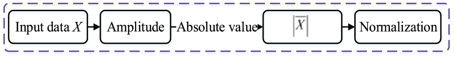
Procedure for data pretreatment.
HI extraction
Extracting the preliminary HI through the DBN.
The dataset
In the pre-training phase of the DBN, the RBM unit of the hidden layer maps the input data to nonlinear space. The pre-training phase is forward-greedy learning. The RBM is trained layer by layer.
In the fine-tuning phase, the DBN adjusts the network parameters to reduce the reconstruction error between the input and output. The DBN adjusts the network parameters to create a probability distribution with the best possible match with the input distribution. Each layer of the DBN is trained by maximizing the likelihood function. In addition, the DBN can simultaneously perform feature dimension reduction operations during the feature extraction process. Therefore, the number of output neuron nodes of the last RBM unit is set to 1, which is the dimension of the extracted HI. The calculation process is as follows.
The idea of the RBM is derived from the energy function. The energy function is optimized using a Boltzmann machine and a generative random network. Each RBM is composed of two layers: a visible layer
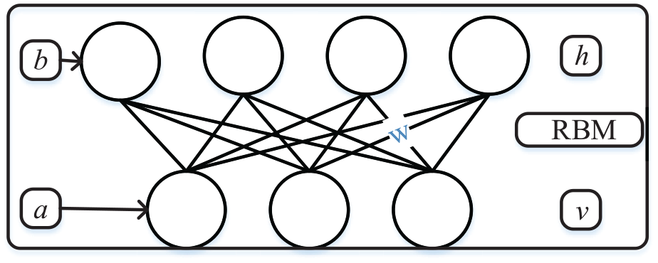
Basic structure of RBM.
The different layers of neurons between v and h are connected to one another, and the neurons inside v and h are independent and unconnected. v is used to connect the original input data and h receives the output of the previous RBM unit; h is the extracted feature of the current RBM; the output h at a hidden layer of the last RBM in this article is the extracted HI, which we called DBN–HI. The neurons in v and h take the values “1” and “0” to represent active and inactive states. The energy function between v and h is
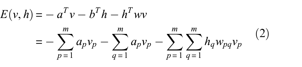
where a is the bias term for v, b is the bias term for h, and
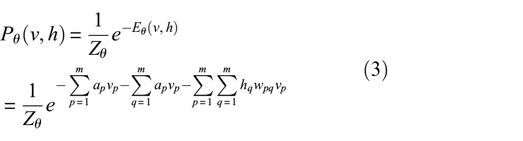
where
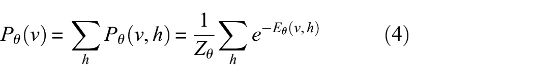
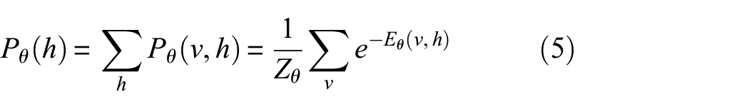
Because the neurons inside v and h in RBM are independent and not connected, the conditional probability distributions of v and h are independent
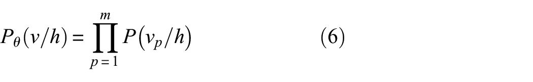
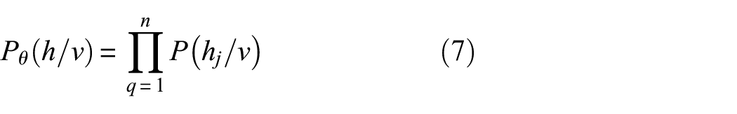
Then, the extracted HI is calculated by
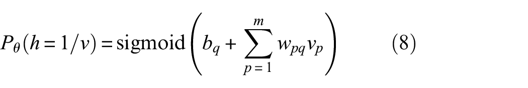
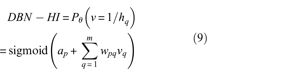
where sigmoid is the activation function
The DBN adjusts the network parameters so that the probability distribution matches the input data distribution as closely as possible, that is, each RBM unit is trained by maximizing the likelihood function below
The DBN uses the Markov chain Monte Carlo (MCMC) method to find the maximum-likelihood function for equation (10), but it uses a long training time and a slow process, which are problems. Usually, the contrastive divergence (CD) algorithm proposed by Hinton, called the CD-k algorithm, is used to solve this problem. Using the CD-k algorithm updates, the weight w and the bias (a, b) are calculated as 26
where
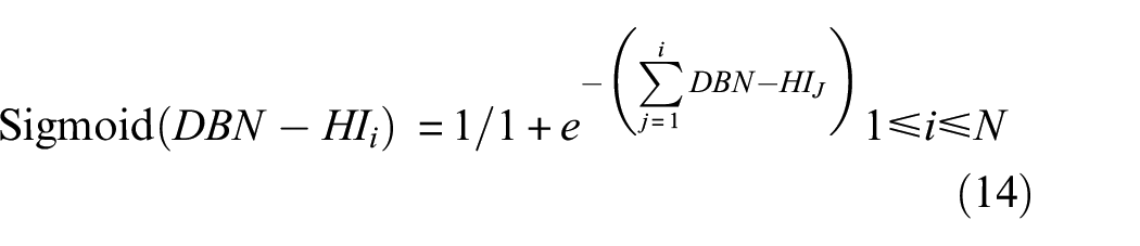
(2) The SZLMP is used to improve the monotonicity of HI. The main idea of the SZLMP is to use the average value from the first HI to the current HI as the input of the sigmoid function to first calculate the initial HI value. This operation reduces the weight of the current HI value, especially when the current HI value jumps significantly. The zero and local minimum data points are then used to replace the HI curve when there is a significant jump and to improve the monotonicity. We call this the DBN–SZLMP–HI. In the following experimental section, we use one bearing as an example to show the detailed calculation step of the SZLMP.
Performance evaluation
The Mon index is used to evaluate the monotonicity of the extracted HI for different models, such as RMS, Kurtosis, AE, PE, various time–frequency indicators in the study by Tse and Wang,
7
EMD–SVD–K-means/K-medoids in the study by Rai and Upadhyay,
10
unsupervised DBN and the SAE with output label layer in the study by Xu et al.
27
Mon mainly uses the difference between the two adjacent HI points to evaluate the monotonicity of the curve. If the difference between the two adjacent points is greater than 0, the straight line between the two points is rising, hence it is monotonically increasing. Conversely, if the difference in time between the two adjacent points is less than 0, and the straight line between these two points is falling; it is monotonically decreasing. The closer the Mon value is to 1, the better the monotonicity. For the given HI dataset
where DA and DB are the total numbers of DF > 0 and DF < 0, respectively.
Experimental setup
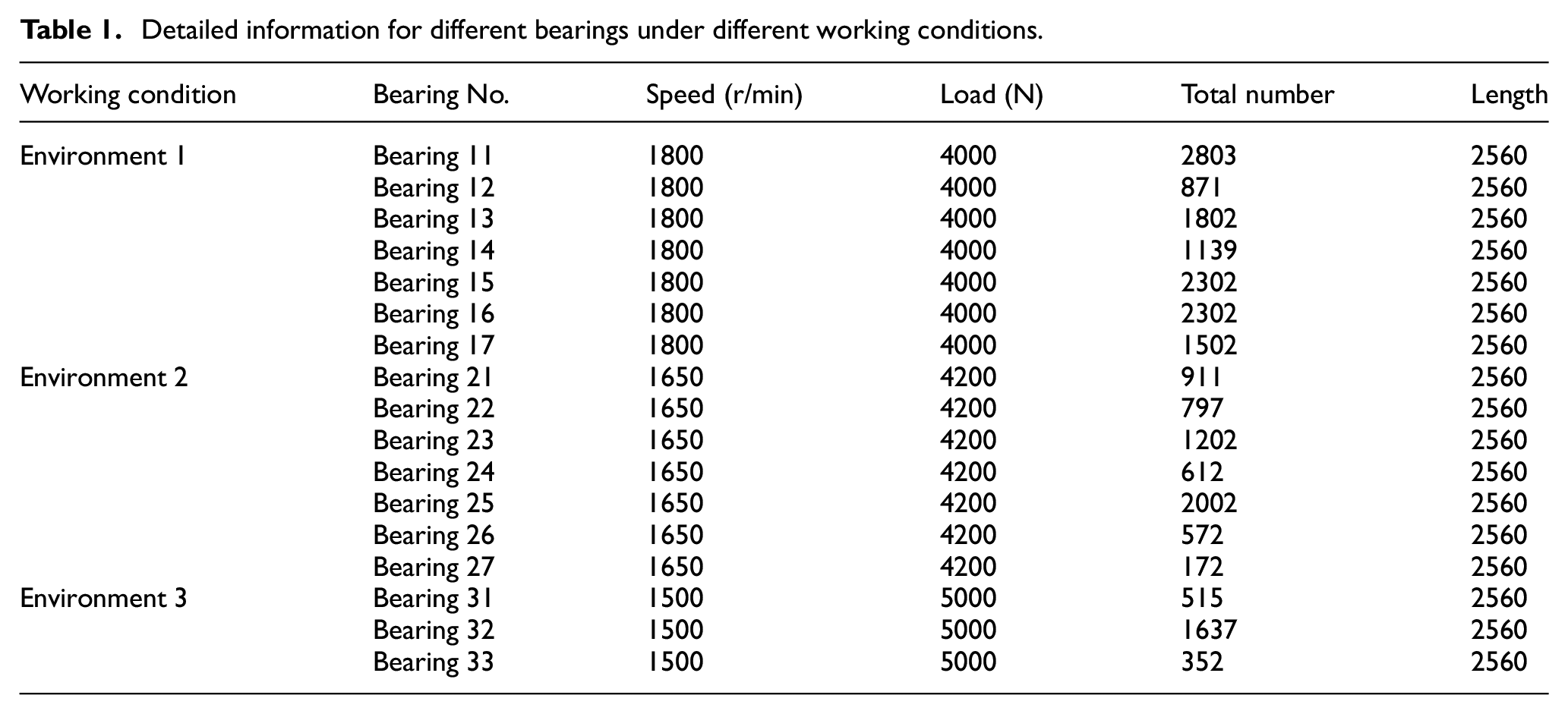
The experimental platform is shown in Figure 5, the bearings exhibited normal to severe wear. The experimental data were collected in three different environments. Environment 1: the bearings were run at a rotation speed of 1800 rotations per minute (r/min) and a load of 4000 N. There were seven bearings. Environment 2: the bearings were run at 1650 r/min, 4200 N, and there were seven bearings. Environment 3: the bearings were run at 1500 r/min, 5000 N, and there were three bearings. The experimental sampling frequency was 25.6 kHz, each sample was collected every 10 s, hence the length of each sample was 2560 points. Detailed information about the experimental data is shown in Table 1.
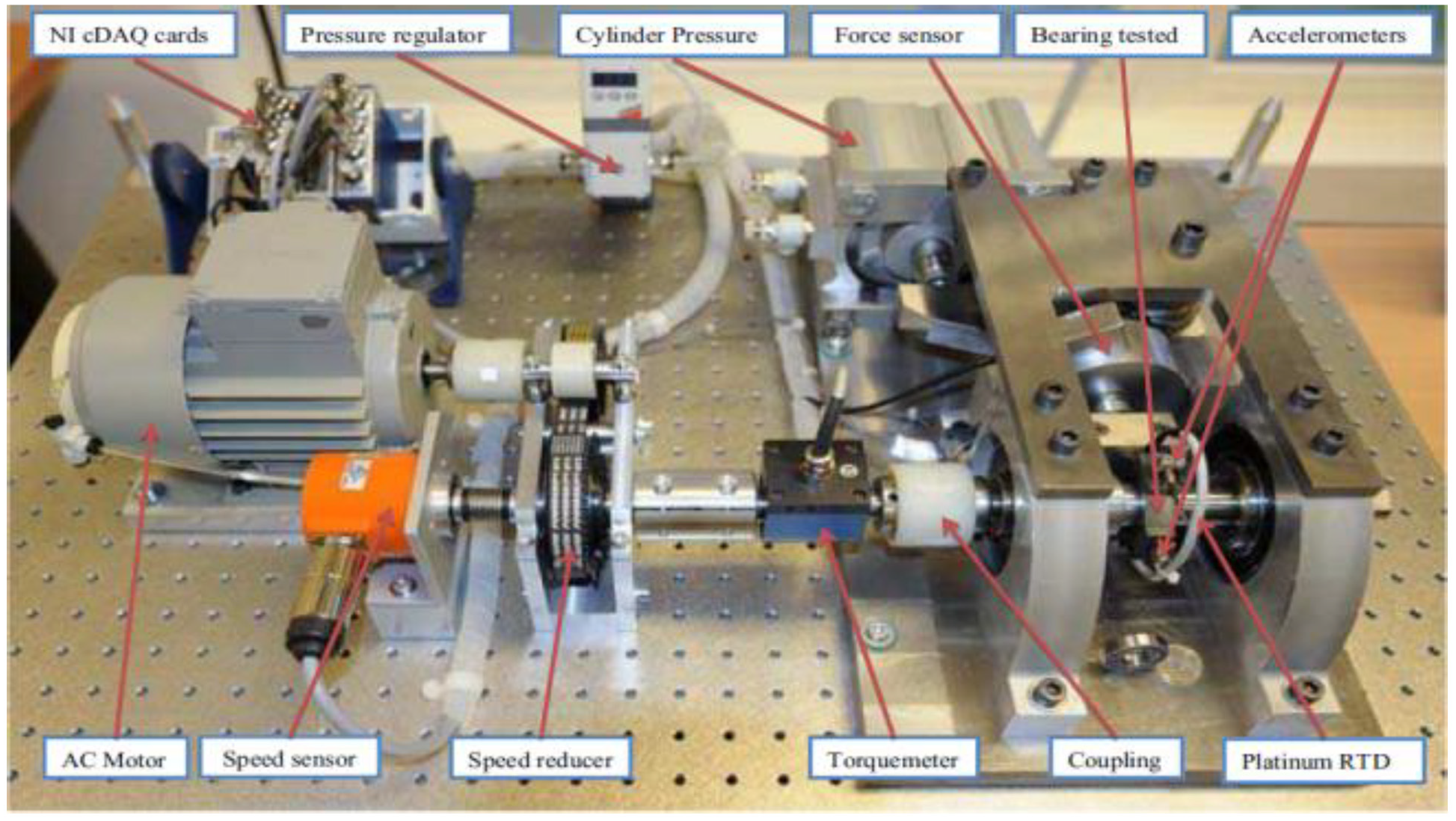
Experimental platform. RTD: resistance temperature detector.
Detailed information for different bearings under different working conditions.
Bearing 13, bearing 14, bearing 23, bearing 44, bearing 25 and bearing 33 were used to compare and analyze the experimental results. The original signals from these six bearings are shown in Figure 6. The rectangular area in Figure 6(b), (c), and (e) shows that the original vibration signal contains a lot of noise. The HI curve was generated with poor smoothness and monotonicity from this noise. Therefore, the SZLMP was used to eliminate the oscillation after the DBN had been used.
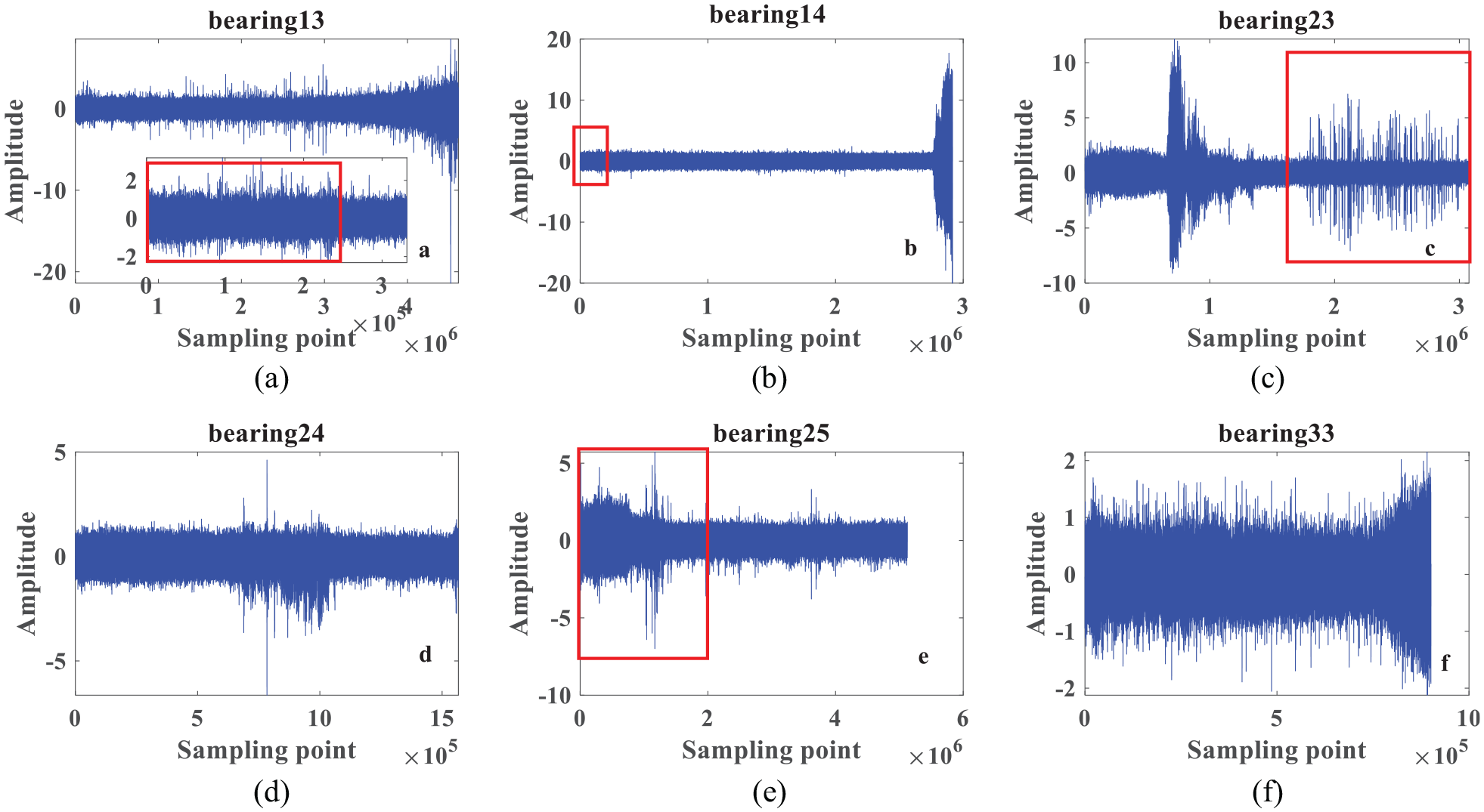
Original time wave signal of different bearings: (a) bearing 13, (b) bearing 14, (c) bearing 23, (d) bearing 24, (e) bearing 25, and (f) bearing 33.
We first used bearing 14 as an example to conduct a comparative analysis of the experiment, and then the other bearings were also used to demonstrate that the performance of our proposed method was better than other models. Table 1 shows 1139 samples for bearing 14. To facilitate the batch processing of the DBN, the first 1100 samples were selected, and each sample was 2560 points in length. During the data initialization phase, each sample was divided into 2560/64 = 40 points, hence the length of each sample was changed to 64, and the total input data sample for the DBN model, when bearing 14 was used, was 1100 × (2560/64) = 44,000 points. Each sample corresponded to a generated HI value of 1, hence the total number of HI was 44,000. Finally an average value was calculated from values sampled at every 40 intervals to generate the final DBN–HI value. Hence the total number of DBN–HI was still 1100. According to the data-preprocessing steps in Section 2.1, the absolute value of the vibration amplitude of each sample was obtained and normalized using equation (1). Because the length of each sample was 64, the input layer size of the DBN was set to 64.
For the DBN hidden layer network structure, research11,12,33–39 has shown that using triangle-based structures can extract fault features effectively and reduce data dimensionality at the same time. Here, the triangle structure represents the number of neuron nodes in the next RBM as half of the preceding RBM. Therefore, the number of neuron nodes at each RBM unit was set to [32 16 8 4 2 1], and there were six RBM units in total (L = 6 in Figure 2).
For the learning rate, Xu et al.
27
showed that setting the learning rate

The following uses bearing 14 to explain how to use the SZLMP model to calculate and extract the HI model.
For bearing 14, the sequence
(2) Calculate the slope K of each data point of
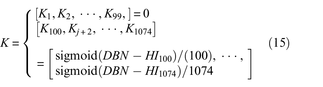
Figure 7 shows that DBN–HI has obvious violent oscillations for the first 120 data points. Because bearing 14 was not fully adapted to the mechanical equipment in the beginning stage, it generated concussion. Hence, because the vibration amplitude of bearing 14 was too great, there was violent vibration within a short period. As time passed, the bearing gradually became fully integrated with the mechanical equipment, and the vibration stabilized. Therefore, the subsequent vibration amplitude rose steadily. However, the short-term oscillation at the beginning stage affected the prediction of the remaining useful life of the bearing negatively. Compared with the smoothness and monotonicity of the DBN–HI curve in Figure 7(b), that of the DBN–SZLMP–HI is better because the SZLMP uses the average value to reduce the dependence on the HI value at the current time to weaken the oscillation.
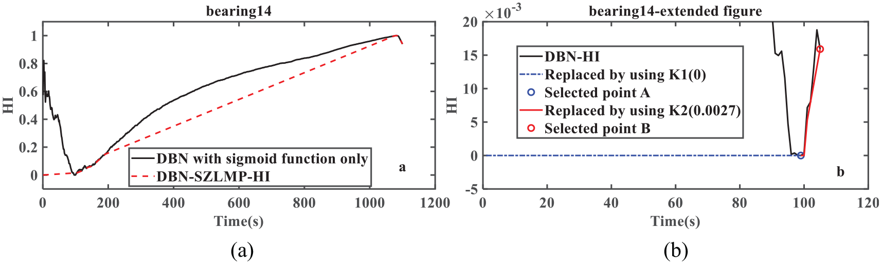
(a) Results of DBN–HI and DBN–SZLMP–HI for bearing 14. (b) Extended SZLMP figure when the first 100 points from the DBN–SZLMP–HI curve are used.
Figure 7(b) shows an enlarged view of the first 120 data points for Figure 7(a). Figure 7(b) shows that the first to 99th HI values are set to 0 (blue dotted line), here K1 = K99 = 0. It significantly reduced the violent oscillation of the first 99 data points. Then, starting from the 99th data point to the 1074th data point, the SZLMP model cyclically connects two adjacent local minimum data points. For example, the first and second adjacent two local minimum data points are 99 and 105 (the red dotted line in Figure. 7(b)), and the slope of the curve is K2 = 0.0027 through these two data points. Figure 7(b) shows that the DBN–HI curve from the 99th data point to the 1074th data point is replaced, and the oscillation declines.
The following uses bearing 14 as an example to illustrate how the HI extracted by the DBN with SZLMP can effectively reflect the health status of the bearing, eliminate concussion, and improve monotonicity. The HI extracted using the DBN and the DBN with SZLMP is shown in Figure 8.
Figure 8(a) shows that bearing 14 begins to enter an abnormal state at the 2774e+06th data point. Because the length of each sample for bearing 14 is 2560, the corresponding extracted HI number is 2.774e+06/2560=1083.6 (an integer value of 1084 is used). This indicates that the bearing began to enter an abnormal state at the 1084th HI point. Figure 8(b) shows that the HI curve using the DBN increases significantly at the 1084th data point (0.2016), whereas Figure 8(c) shows the HI curve using the DBN with SZLMP has an obvious inflection point at the 1084th HI point. Because the SZLMP model first uses the average value of all HI points from the start time to the current time to calculate the final current HI value, which reduces the weight of the current HI value, as shown in Figure 8(b), there is a significant increase at the 1084th HI point (0.2016). However, the SZLMP uses the average value from the start time to the 1084th HI point to calculate the final HI value, hence the calculation weight of the 1084th HI value is assigned to 1/1084, which weakens the 1084th HI value in Figure 8(b). Therefore, Figure 8(c) shows that there are no strong rises or falls at the 1084th HI point. This shows that the use of the DBN and the DBN with SZLMP models can effectively reflect the health status of the bearing.
Compared with the DBN, the monotonicity of the HI curve extracted by the DBN with the SZLMP model is good. As shown in Figure 8(b), the HI curve is basically stable before the 1084th HI point. On the contrary, the HI curve in Figure 8(c) maintains a steady growth trend. Hence this result lays a good foundation for subsequent life prediction. Figure 8(c) shows that after using the SZLMP model, the oscillation of the first 120 HI points obviously disappears. This result shows that the SZLMP can effectively eliminate shocks and improve the monotonicity of the HI curve.
Here, we take a picture as an example to illustrate the advantages of constructing a good monotonic HI curve, and further explain how the HI curve is used for life prediction. The specific steps are as follows.
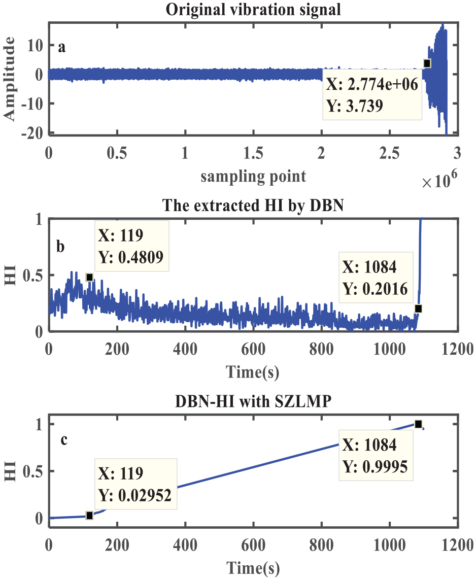
Extracted HI from the DBN and the DBN with SZLMP using the original signal. (a) Original vibration signal, (b) the DBN–HI, and (c) the DBN–SZLMP–HI.
The first step is to divide the HI points into the training data and testing data of the prediction model. For example, the first 200 HI points were selected as the training data, and the rest of the HI points were used as the testing data, but there is no unified theoretical standard for threshold setting, which is generally set by manual experience. The second step is to predict the remaining life using the testing data. When the predicted HI value exceeds the set threshold at time t, the remaining life of one bearing is calculated as t − 200.
In Figure 9, the blue curve is the predicted value, the red curve is the actual value, and the black curve is the threshold. The blue curve in the blue rectangular area exceeds the threshold curve. However, the HI curve in the blue rectangular area during life early stage is selected as training data. Therefore, these life early stage HI points are not considered in this article. If the monotonicity of the early HI curve is poor (blue area), it is difficult for the predicted HI value to exceed the threshold line. In addition, because the real HI value (red curve) oscillates slightly in the early stage, the early HI prediction curve (blue curve in the blue area) first falls and then rises. Therefore, it is necessary to use the SZLMP model to improve the monotonicity of the HI curve and eliminate the oscillation phenomenon.
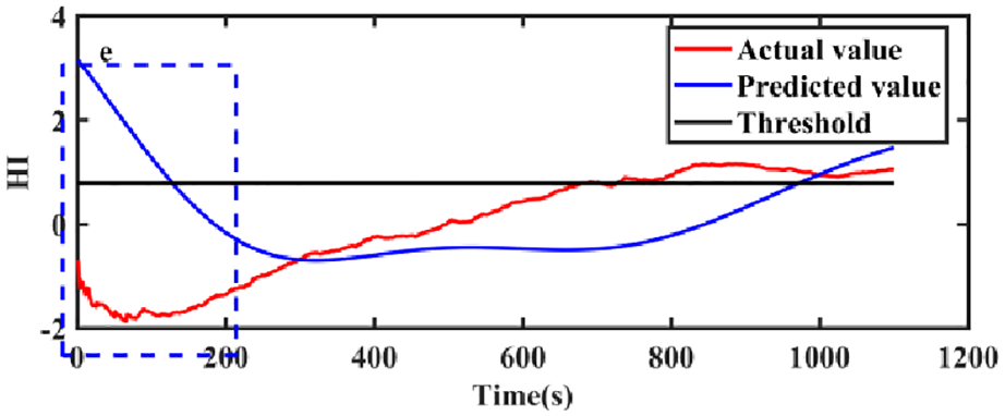
Example to explain “How to use HI curve fulfilling the remaining useful life prediction and the advantage of the SZLMP.”
In order to further verify that the effectiveness of the DBN–SZLMP is superior to that of other models, such as RMS, Kurtosis, AE, PE, various time–frequency indicators in the study by Tse and Wang, 7 EMD–SVD–K-means/K-medoids in the study by Rai and Upadhyay, 10 and the unsupervised DBN and the SAE with output label layer in the study by Xu et al., 27 the Mon index is used to evaluate the monotonicity of the HI curve. The HI curve and Mon results generated by the above model are shown in Figure 10 and Table 2.
Figure 10 shows that the smoothness and monotonicity of the DBN–SZLMP–HI curve are significantly better than those of other models, especially the DBN–HI, AE, and PE, because there is obvious noise. The DBN–SZLMP–HI curve also gradually increases. Furthermore, the HI curves generated by the DBN–SZLMP–HI and SAE–EHI are similar to each other when viewed with the naked eye. Hence the smoothness and monotonicity of the HI curve generated by using these two models are good, but the SAE–EHI model needs manual experience for labeling the data, whereas the unsupervised DBN does not. Moreover, the data preprocessing requires fast Fourier transformation (FFT) to transform the data from the time domain to the frequency domain, hence the data preprocessing process in the study by Xu et al., 27 is complicated. Therefore, compared with the SAE–EHI model, the DBN–SZLMP in this study does not require FFT transformation, and its data preprocessing procedure is simple.
In order to verify the superiority of the DBN–SZLMP further, the Mon index is used to evaluate the monotonicity of the HI curves generated by different models. Table 2 shows that the greatest Mon value is 0.9672 (DBN–SZLMP), and the minimum Mon value is 0.0088 (Kurtosis).
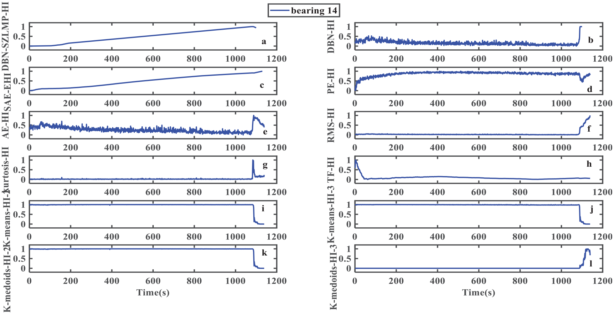
Results of HI for bearing 14 extracted through different models: (a) DBN–SZLMP; (b) DBN without an output layer; (c) SAE–EHI in the study by Xu et al.; 27 (d) PE; (e) AE; (f) RMS; (g) Kurtosis; (h) various time–frequency indicators in the study by Tse and Wang, 7 TF denotes the time–frequency; (i, j) K-means (K-means denotes the EMD–SVD–K-means) (2/3) in the study by Rai and Upadhyay, 10 “2” and “3” denote the cluster numbers 2 and 3, respectively; (k, l) K-medoids (K-medoids denotes the EMD–SVD–K-medoids) (2/3) in the study by Rai and Upadhyay. 10
Results of Mon using different models for bearing 14.
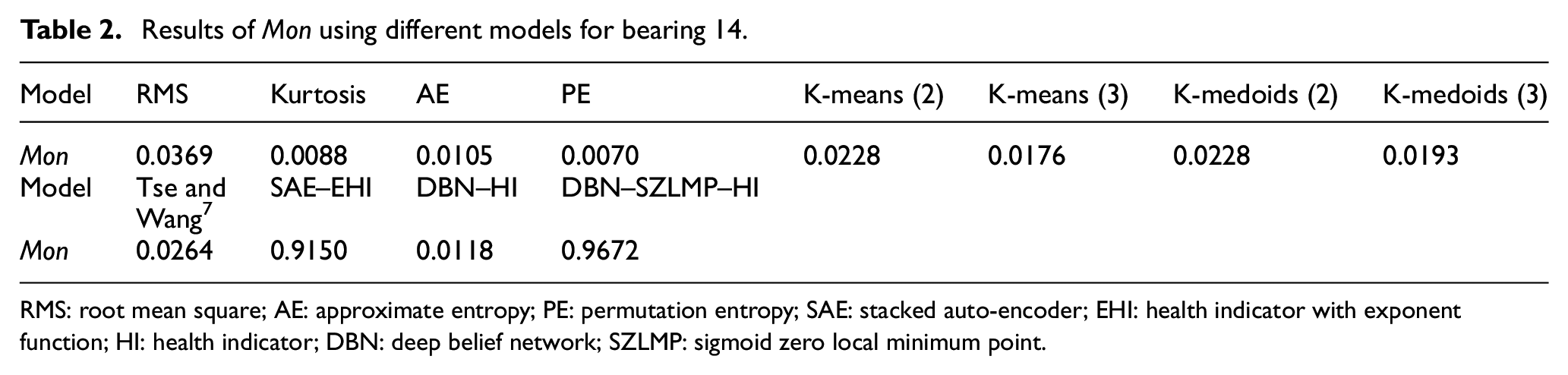
RMS: root mean square; AE: approximate entropy; PE: permutation entropy; SAE: stacked auto-encoder; EHI: health indicator with exponent function; HI: health indicator; DBN: deep belief network; SZLMP: sigmoid zero local minimum point.
The above model was applied to other bearing datasets to further verify the superiority of the model. The model parameters remained unchanged. The generated HI curves and Mon results for bearing 13, bearing 23, bearing 24, bearing 25, and bearing 33 are shown in Figure 11 and Table 3.
Figure 11 shows that the smoothness and monotonicity of the DBN–SZLMP–HI curve are significantly better than those of other models, especially the DBN–HI, AE, and PE. The HI curves generated by the DBN–SZLMP–HI and SAE–EHI are similar when viewed with the naked eye. However, the DBN–SZLMP–HI model is slightly superior to SAE–EHI, for example, bearing 25 (yellow curve) as shown in Figure 11(c). The DBN–SZLMP–HI curve gradually increases over time. Conversely, the SAE–EHI curve starts at the 300th data point, remains stable, and has no obvious upward trend, hence the monotonicity is poor. However, the SAE–EHI model requires manual experience to label the data.
Table 3 shows that the greatest Mon value, except for bearing 33, is 1 (DBN–SZLMP). The Mon value of the DBN–SZLMP is significantly higher than that of other models. Although the Mon value (0.7536) of bearing 33 is less than that of SAE–EHI (0.810), it is close to 0.810.
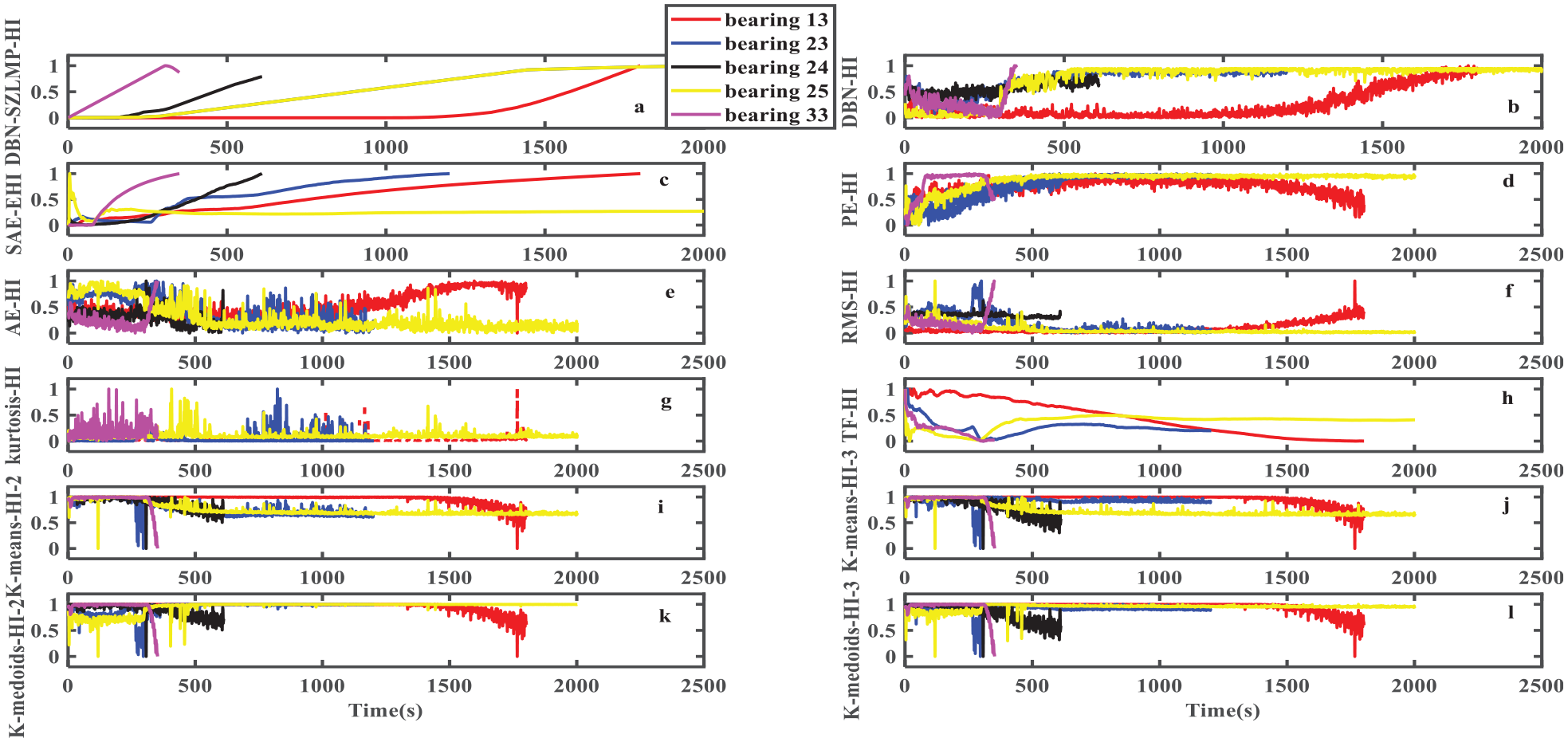
Results of HI extracted using different models for bearings (bearing 13, bearing 23, bearing 24, bearing 25, and bearing 33). (a) DBN–SZLMP; (b) DBN without output layer; (c) SAE–EHI in the study by Xu et al.; 27 (d) PE; (e) AE; (f) RMS; (g) Kurtosis; (h) Various time–frequency indicators in the study by Tse and Wang, 7 TF denotes the time–frequency; (i, j) K-means (K-means denotes the EMD–SVD–K-means (2/3) in the study by Rai and Upadhyay, 10 “2” and “3” denote the cluster numbers 2 and 3, respectively; (k, l) K-medoids (K-medoids denotes the EMD–SVD–K-medoids( (2/3) in the study by Rai and Upadhyay. 10
Results of Mon through different models for various bearings (bearing 13, bearing 23, bearing 24, bearing 25, and bearing 33).
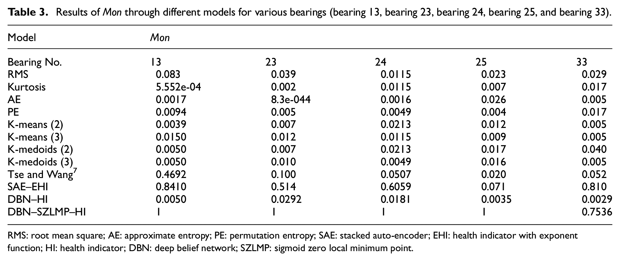
RMS: root mean square; AE: approximate entropy; PE: permutation entropy; SAE: stacked auto-encoder; EHI: health indicator with exponent function; HI: health indicator; DBN: deep belief network; SZLMP: sigmoid zero local minimum point.
These results show that the model proposed in this study is better than the other models.
Conclusion
This study proposed a DBN and SZLMP-based method to improve the smoothness and monotonicity of the HI curve. To reduce the dependence on manual experience, a DBN without an output label layer was used to extract the preliminary HI directly from the original bearing data. In order to further eliminate the problem of concussion in the extraction of the HI curve because of noise in the actual engineering, a new SZLMP model was proposed. The SZLMP used the average value from the start time to the current time to reduce the dependence weight of the current HI value to eliminate concussion, then used the local minimum data points with no parameter settings to improve the monotonicity of HI further. Multiple bearings were compared to verify the superiority of the model.
In addition, we will focus on the study of life prediction models in future research. Commonly used life prediction models are long short-term memory (LSTM), relevance vector machine, Kalman filtering, and the particle filter. LSTM, in particular, has the advantages of multiple hidden layers of time-series memory units. When there is noise in the time series, it is generally necessary to use a denoising model to perform a denoising operation on the time series during the data preprocessing stage. In response to this defect, we intend to add the denoising model behind the multiple hidden layers of the LSTM to perform multiple denoising steps on the time series. Therefore, an LSTM model with a denoising operation will be proposed and compared with other prediction models (such as relevance vector machine, Kalman filtering, and the article filter) in future research.
Footnotes
Declaration of conflicting interests
The author(s) declared no potential conflicts of interest with respect to the research, authorship, and/or publication of this article.
Funding
The author(s) disclosed receipt of the following financial support for the research, authorship, and/or publication of this article: This research work was partly supported by the National Natural Science Foundation of China (Grant No. 51909199), the National Natural Science Foundation of China (Grant No. 51709215).