Fatigue damage diagnosis and prognosis of an aeronautical structure based on surrogate modelling and particle filter

Abstract

A key issue affecting the performances of every human-conceived engineering system is its degradation, fatigue crack growth being one of the major structural deterioration phenomena. Fatigue crack growth is usually modelled as a stochastic process: uncertainty sources lie both in the item and in the physical degradation process variability. Fatigue crack growth deserves close attention, especially considering that condition-based maintenance methodologies are recently experiencing a major drive to increase their technology readiness level, requiring validated diagnostic and prognostic methodologies which should be capable of operating online and in real-time. In this regard, particle filters provide a consistent Bayesian framework, where the posterior distribution of the system degradation state is recursively approximated based on a time-growing stream of observations measuring the system response, enabling, in general, increasingly informed lifetime estimates. However, the real-time operation capability of such methods is hindered by their requirements in terms of computational power, which is mainly due to the complexity of the structural models they rely upon. Within this work, a comprehensive particle filter framework, able to deal with fatigue crack growth uncertainty sources while simultaneously addressing the computational burden issue, is proposed. The algorithm structure enables to simultaneously perform the diagnosis and prognosis of fatigue crack growth, while the adoption of the augmented state formulation allows to address scenarios where the degradation process of fatigue crack growth fails to meet the degradation model ruling the particle filter. Artificial neural networks–based surrogate modelling is adopted at different stages and embedded within the particle filter algorithm, relieving the computational burden associated with the evaluation of the trajectory likelihoods as well as enabling a fast estimation of the remaining useful life. Both simulated and experimental data sets regarding fatigue crack growth in an aluminium aeronautical panel are used for the algorithm testing, additionally proving the validity and effectiveness thereof by means of common prognostic performance metrics.

Keywords

Particle filter fatigue crack growth damage diagnosis damage prognosis remaining useful life surrogate modelling artificial neural networks

Introduction

Structure degradation phenomena, such as fatigue, pose a serious threat to the structural integrity of many systems, especially those subject to strict weight constraints and severe load spectra, such as aerial vehicles: these conditions, in fact, lead in general to highly stressed structures, which, at the same time, are required to comply with severe safety requirements.^1,2 This, in turn, entails frequent overhaul and idle times, resulting in serious running costs, which are distinctive of the traditional maintenance strategies. The possibility of accurately estimating the system remaining useful life (RUL) would allow a paradigm shift in the assets maintenance procedures, meaning that the traditional scheduled maintenance practices (preventive maintenance) could evolve towards condition (and even prediction)-based maintenance (CBM) philosophies, where the assets are maintained based on their estimated current condition rather than based on scheduled intervals, ensuring reduced maintenance-related costs and increased system safety and availability at the same time. CBM requires that proper diagnostic and prognostic tools are developed to obtain an accurate picture of the health state of the system critical components (diagnosis) as well as an estimate of the components RULs (prognosis).³

As with diagnostics, prognostics methods are usually classified as either data-driven or model-based.^4–6 Data-driven approaches leverage on the availability of run-to-failure data, targeting hidden patterns unveiling the relationships between observable system features, that is, vibration amplitude, and RUL or end of life (EoL) variables.⁷ However, despite their ability to mine data looking for patterns, data-driven approaches might be limited by data availability. Model-based approaches, instead, take advantage of the available knowledge about the system degradation behaviour, exploiting the underlying principles driving the physics of the problem, exhibiting increased robustness and flexibility, as well as enhanced accuracy and precision, provided that the models are consistent with the observed phenomena and that some features related to the degradation state can be measured.⁸ However, real-world RUL estimates might be difficult to obtain, since measurements are almost always noisy, and features relating to the RUL estimates are usually not directly observable; generally, RUL can be treated as a random variable.⁹ Prognostic tools should also be designed in a way that reliable RUL estimates are provided in conditions of limited sensing.¹⁰ Also, it is not unusual that evolution models driving parameters are not exactly known, due to inter-item material variability.¹¹ In these circumstances, model-based methods targeting the hidden degradation state variables on the basis of a noisy stream of observations and, at the same time, offering a quantitative perspective of the estimates uncertainty, provide an interesting alternative.

Such methods are naturally suited to be looked at in a Bayesian perspective, in which the actual knowledge about the system health status – and consequently about the RUL estimate – is sequentially updated as soon as new observations are collected, targeting the posterior probability density function (pdf) of the system damage states, conditional on the stream of gathered observations. Specifically, sequential Monte Carlo (SMC) methods – which include particle filters (PFs) – offer a consistent framework, able to deal with non-linear state evolution models and non-Gaussian observation/process noise.^12–16 A few applications of the PF handling various degradation phenomena – including fatigue crack growth (FCG) – are illustrated in the literature.^17–20 PF has been also successfully employed in several situations for condition assessment of vibrating systems; meaningful examples are described in the literature.^21–24

In the literature, diagnostics and prognostics are usually performed separately, relying on dedicated tools. More specifically, the PF is often confined to prognostics only, and its diagnostic capabilities are often neglected. Within this work, we propose a PF algorithm which performs both the diagnosis and prognosis with reference to an FCG problem. Specifically, a sequential importance resampling (SIR) PF algorithm is implemented, and experimental strain measurements are exploited to estimate the system degradation state, that is, the crack size and location. The deterministic degradation model is based on the Paris’ Law.²⁵ However, due to the inherent stochastic nature of FCG,^26,27 which is due to variability affecting material properties and the degradation process, the deterministic degradation model is turned into a stochastic one. Uncertainty in the material properties is here addressed by ‘augmenting’ the state space with the material parameters influencing the degradation model. Therefore, the state space has been expanded to combine the crack state variables with the evolution model parameters.

PFs are required to operate in real-time, meaning that the stream of data that is collected at each observation time needs to be processed within the time elapsing between contiguous observations. Therefore, it is crucial to adopt measures to ensure adequate processing capabilities. Within the present context, the most time-demanding tasks are the likelihood assessment and the particles trajectories evaluation for the RUL estimates. Being in a model-based environment, these duties require that structural models of the system under study are run several times, hindering the real-time operation of the PF. In this work, we propose to address this issue by adopting surrogate models in place of the computationally demanding high-fidelity structural models.^28,29 Specifically, offline trained artificial neural networks (ANNs) are exploited, linking the degraded system state (i.e. crack state variables) with the measured features (i.e. strain), driving the likelihood assessment. Training data sets are generated offline via a set of finite element models (FEMs) accurately reproducing the system of interest by varying the crack state variables. Similar approaches are illustrated in the literature,^24,30,31 where surrogate models are used to advance repeated computational procedures. Surrogate models are also exploited for the particles RUL estimates, by providing the crack stress intensity factors (SIFs) – one for each crack tip – as a function of the crack state variables. In literature, several works address the problem of building surrogate models for the SIF determination, exploiting distinct techniques, intending to reduce the computational efforts which are related to the FCG simulation.^32–36

This article is structured as follows: the theoretical background concerning the PF algorithm is introduced in section ‘Theoretical background’, including a subsection dedicated to surrogate modelling viewed as a good practice aimed at enhancing the real-time capabilities of the PF. Section ‘Application to FCG’ deals with the implementation of the PF within the practical case of the FCG scenario, evaluating the algorithm potential via prognostic performance metrics in a real test case when challenged with experimental data, repeated on a set of four identical units. Finally, conclusions are drawn, and future extensions of the method are discussed.

Theoretical background

The objective of the filtering problem is to recursively estimate the augmented state of a system, including $n_{x} (n_{x} \in N)$ state variables $x$ and a vector of $n_{ϑ} (n_{ϑ} \in N)$ parameters $ϑ$ , conditional on a set of noisy observations $z$ . This system is governed by a dynamic state space (DSS) model which includes the evolution equation, $f (\cdot)$ , describing the system dynamics, that is, the system degradation model, and the observation function, $g (\cdot)$ , which links the measurements with the true (hidden) system state. Equation (1) shows the discrete form of the DSS model, which satisfies the first-order Markovian assumption¹⁴

\begin{matrix} y_{k} = f (y_{k - 1}, u_{k - 1}, ω_{k - 1}), y_{k} = {[x_{k}, ϑ_{k}]}^{T} \\ z_{k} = g (y_{k}) + η_{k} \end{matrix}

(1)

The vector $y \in D_{y} \subseteq ℝ^{n}$ collects the system augmented state variables, with $n = n_{x} + n_{ϑ}$ , $z = [z_{1}, z_{2}, \dots, z_{s}]^{T} \in D_{z} \subseteq R^{s}$ being the observation vector, $s \in N$ being the number of sensors, and the subscript $k$ is the discrete kth time step ( $k \in N$ , $k = 1, \dots, N_{obs}$ ). The state-space domain $D_{y}$ is the physical domain of the system augmented state variables, represented by a partition of the set $R^{n}$ .

The evolution function depends on the input u , the model parameters $ϑ$ and the process noise, $ω$ . A common assumption is that the input of the system u is observable, and its observability is not further discussed henceforth. The measurement equation is governed by $g (\cdot)$ and affected by the measurement noise, $η$ (e.g. electrical noise and environmental noise). The noise terms $ω$ and $η$ are random variables transforming the deterministic equations in equation (1) into stochastic equations. Note that the system response $z_{k}$ is a function of the system state $x_{k}$ only, thus we can write the measurement equation in the following form: $z_{k} = g (x_{k}) + η_{k}$ .

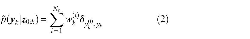
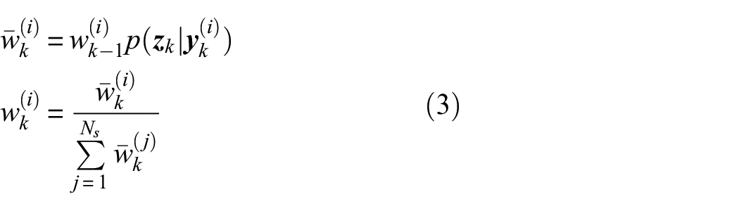
Particle filtering aims at estimating the posterior pdf of $y_{k}$ given the sequence of noisy observations $z_{0 : k}$ , $p (y_{k} | z_{0 : k})$ , in case of non-linear and non-Gaussian systems. The posterior pdf can be approximated by $N_{s}$ weighted samples (also called particles) of the system’s state, as expressed in equations (2) and (3)^13,14

\hat{p} (y_{k} | z_{0 : k}) = \sum_{i = 1}^{N_{s}} w_{k}^{(i)} δ_{y_{k}^{(i)}, y_{k}}

(2)

\begin{array}{l} {\bar{w}}_{k}^{(i)} = w_{k - 1}^{(i)} p (z_{k} | y_{k}^{(i)}) \\ w_{k}^{(i)} = \frac{{\bar{w}}_{k}^{(i)}}{\sum_{j = 1}^{N_{s}} {\bar{w}}_{k}^{(j)}} \end{array}

(3)

where $\hat{p} (y_{k} | z_{0 : k})$ is the approximation of $p (y_{k} | z_{0 : k})$ , $y_{k}^{(i)} = [x_{k}^{(i)}, ϑ_{k}^{(i)}]^{T}$ is the ith sample of the system’s augmented state vector, $w_{k}^{(i)}$ is the normalized weight of $y_{k}^{(i)}$ , $p (z_{k} | y_{k}^{(i)})$ is the likelihood of the observation given $y_{k}^{(i)}$ and $δ_{\cdot, \cdot}$ is the Kronecker delta. The number of samples $N_{s}$ is supposed to be large enough to describe the (unknown) exact shape of $p (y_{k} | z_{0 : k})$ . It should be noted that equations (2) and (3) refer to the bootstrap PF.¹⁴

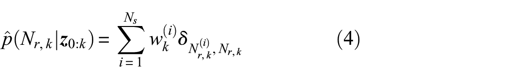
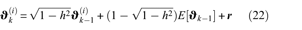
The particle filtering–based prognosis is carried out by projecting the samples $x_{k}^{(i)}$ , $i = 1, \dots, N_{s}$ many steps ahead in the future, up to a limit state condition, with the p-step ahead prediction equation,¹³ taking the input u , the evolution model parameters $ϑ$ and the process noise $ω$ , into account. In a scenario for damage evolution prognosis under fatigue load cycles, the posterior pdf of the number of remaining load cycles $N_{r, k}$ to the critical condition can be estimated at discrete time k as reported in equation (4)

\hat{p} (N_{r, k} | z_{0 : k}) = \sum_{i = 1}^{N_{s}} w_{k}^{(i)} δ_{N_{r, k}^{(i)}, N_{r, k}}

(4)

where $N_{r, k}^{(i)}$ is the number of remaining load cycles to the limit condition, associated to the ith particle trajectory.

The practical implementation of the algorithm requires the definition of three fundamental functions

The transition density function of the state variables, $p (x_{k} | x_{k - 1}, ϑ_{k - 1})$ , which drives the generation of samples $x_{k}^{(i)}$ and the p-step ahead prediction equation.¹³

The transition density function of the parameters, $p (ϑ_{k} | ϑ_{k - 1})$ , which drives the generation of samples $ϑ_{k}^{(i)}$ , hereafter based on Kernel smoothing approach.³⁷

The likelihood function, $p (z_{k} | y_{k}^{(i)})$ , strictly related to the function $g (\cdot)$ in equation (1) and calculated based on the availability of a surrogate model, as discussed in the next paragraph.

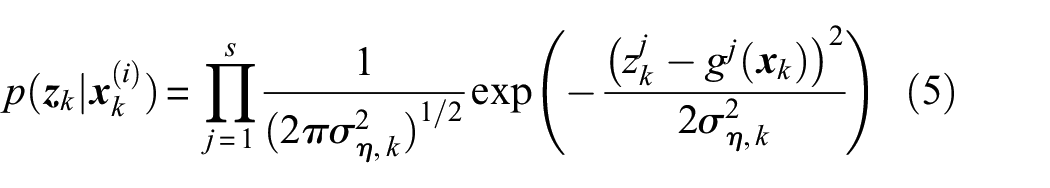
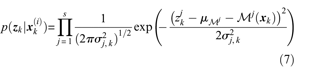
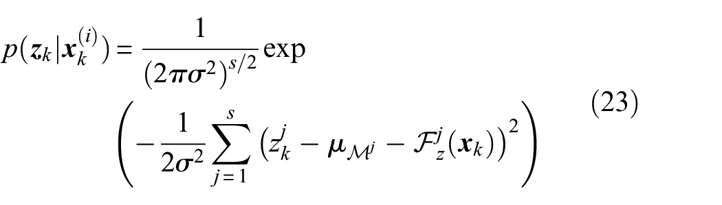
In practice, likelihood calculation is performed based on the observation function $g (\cdot)$ in equation (1), by estimating the system response $g (x_{k})$ corresponding to each sample $x_{k}$ , then quantifying the consistency between the predicted and the measured values via a pdf which is prescribed by the probability distribution of the noise $η_{k}$ . Assuming the noise vector $η_{k}$ to be zero-mean normally distributed and having a diagonal covariance matrix, that is, $η_{k} ~ N (0, σ_{η, k}^{2} I)$ , where $I$ is the identity matrix, the likelihood then reads

p (z_{k} | x_{k}^{(i)}) = \prod_{j = 1}^{s} \frac{1}{{(2 π σ_{η, k}^{2})}^{1 / 2}} \exp (- \frac{{(z_{k}^{j} - g^{j} (x_{k}))}^{2}}{2 σ_{η, k}^{2}})

(5)

where $g^{j} (x_{k})$ stands for the jth element of the response vector $g (x_{k})$ , while $z_{k}^{j}$ is the jth element of $z_{k}$ , and $s$ is the number of observed features, corresponding here to the number of sensors. We can think of the observation function $g (\cdot)$ as the hypothetical operator returning the ground truth value of the system response; in what follows, it will be explained that the task of $g (\cdot)$ is generally performed – with a certain level of approximation – by a model $M$ mapping the state space into the observation space. Superscript (i), indicating the ith state-space sample, that is, the ith particle, is omitted in the left-hand term of equation (5), and, for the sake of clarity, hereafter will be left out if not strictly necessary.

The measurement equation (1) can benefit from any model relating the state variables in $x_{k}$ to the measured features in $z_{k}$ . For instance, if an FEM $M$ is available, we can rewrite the measurement equation as

z_{k} = M (x_{k}) + n_{M} + η_{k}

(6)

where the error term $n_{M}$ accounts for the discrepancy between the approximated system response prediction $M (x_{k})$ and the ground truth represented by $g (x_{k})$ . It is assumed that $n_{M}$ is normally distributed and independent of the system state $x_{k}$ , and that its elements are independent, that is, $n_{M} ~ N (μ_{M}, Σ_{M})$ , where the covariance matrix $Σ_{M}$ is diagonal. The normality assumption for $n_{M}$ allows to readily define the cumulative error $n_{M} + η_{k}$ distribution, that is, $n_{M} + η_{k} ~ N (μ_{M}, σ_{η, k}^{2} I + Σ_{M})$ ; note that the covariance matrix is still diagonal. Equation (5) is updated as follows

p (z_{k} | x_{k}^{(i)}) = \prod_{j = 1}^{s} \frac{1}{{(2 π σ_{j, k}^{2})}^{1 / 2}} \exp (- \frac{{(z_{k}^{j} - μ_{ℳ^{j}} - ℳ^{j} (x_{k}))}^{2}}{2 σ_{j, k}^{2}})

(7)

where the superscript $j$ in $M^{j}$ specifies that we are considering the FEM response in the location corresponding to the jth sensor only. The variance $σ_{j, k}^{2}$ is the jth entry of the resultant covariance matrix $σ_{η, k}^{2} I + Σ_{M}$ , while $μ_{M}^{j}$ is the jth entry of the vector $μ_{M}$ . Note that each FEM estimate $M^{j} (x_{k})$ is affected by its own error distribution $n_{M^{j}} ~ N (μ_{M^{j}}, σ_{M^{j}}^{2})$ , where $n_{M^{j}}$ is the jth entry of the error vector $n_{M}$ comprising $s$ components; this might be the case when the model provides distinct levels of accuracy depending on the position of the sensor. It is also worth noting that the biases related to the model $M$ predictions are taken into consideration by including the mean value vector $μ_{M}$ elements into equation (7)

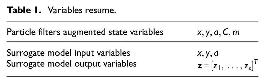
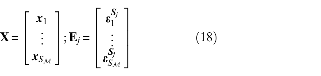
The process in equation (7) is repeated $N_{s}$ times ( $i = 1, \dots, N_{s}$ ) at each kth discrete time ( $N_{s}$ being the number of state-space samples, i.e. particles). In a model-based framework, this means running a simulation each time a new likelihood assessment is required, which is often not feasible if no analytical closed form solution exists for $g (\cdot)$ , as this would lead to very high computational effort, preventing the real-time application of the method. Here, we propose to replace the high-fidelity model $M$ with a surrogate model $F$ , obtaining the approximated response $F (x)$ . Surrogate modelling relies on the offline (i.e. a priori) computation and storage of input-output pairs from the model $M$ aiming at replacing this last with a more time-efficient data-driven model (the surrogate model $F$ ) during the analysis (online). In the application considered here, the model $M$ links the system state $x$ ( $n_{s}$ crack features identifying the system degradation, i.e. crack length and location) to the $s$ strain observations in $z$ (the system response), taken as degradation indicators ( $s$ sensors sampling the strain field at each inspection time $k$ ). Note that the input features in $x$ enter the PF augmented state; in Table 1, a summary of the variables involved is provided. Therefore, the input–output pairs are obtained by evaluating the original model $M$ for $S_{M}$ state samples $x_{i}$ , given $i = 1, \dots, S_{M}$ and $x_{i} \in R^{n_{s}}$ ; therefore, for each input $x_{i}$ , the relative output $M (x_{i})$ is computed, and the input-output pair ${x_{i}; M (x_{i})}$ is stored. This results in an input-output database consisting of an $S_{M} \times n_{s}$ input matrix $X$ and an $S_{M} \times s$ output matrix $E$ , that is, $T = {X; E} = {x_{i}; M (x_{i})}_{i = 1}^{S_{M}}$ is called the training data set. The aim of surrogate modelling is to exploit the stored data to predict the outputs $M (x_{i})$ for new input samples $x_{*}$ ( $x_{*} \notin T$ ) without requiring to evaluate the original model $M$ ; instead the surrogate model $F$ is used, $F (x_{*}) \approx M (x_{*})$ . From a machine learning perspective, a variety of algorithms can be used to infer the input-output mapping by exploiting the training data set in a way that a given function of the error quantity $M (x) - F (x)$ is minimized over test data. In practice, a surrogate model shall recognize and learn the pattern hidden in the training data set, providing a manageable function $F$ replacing the model $M$ , at the expense of reduced accuracy and precision. It is worth mentioning that within this study both the training set and the test set for the surrogate modelling training and testing are generated by uniformly sampling the system state-space domain $D_{x}$ .

Table 1.

Variables resume.

Particle filters augmented state variables	$x, y, a, C, m$
Surrogate model input variables	$x, y, a$
Surrogate model output variables	$z = {[z_{1}, \dots, z_{s}]}^{T}$

From a machine learning perspective, several techniques are at disposal in order to infer the aforementioned input–output mapping, such as linear/polynomial regression, Gaussian processes, neural networks and support vector machines just to mention a few.^28–33 Here, we selected ANNs, as these are known to be universal function approximators and generally give good results on unseen data and are relatively computationally inexpensive to evaluate. Therefore, after evaluating the FEM $M$ at the selected training points $x_{i}$ and having stored the resulting input-output pairs, it is possible to define the ANN architecture. Due to the independence of the output features, two surrogate modelling strategies have been considered as follows

The training data set $T$ is exploited as it is, and one multi-output ANN is obtained, which predicts the set of $s$ strain values for the new input state $x_{*} \notin T$ , $F (x_{*}) \approx M (x_{*})$ .

The data set $T$ is sliced into $s$ subsets $T_{j}$ , where $j = 1, \dots, s$ , and $T_{j} = {X; E_{j}}$ , where $E_{j}$ is the jth column of the matrix $E$ , comprising the response of the jth sensor to the input set $X$ . By adopting this approach, we get $s$ training data sets, and therefore, $s$ single-output ANNs (which we call $F_{z}^{j}$ , where $j = 1, \dots, s$ ) are to be expected, each one predicting the strain for the relative sensor, that is, $F_{z}^{j} (x_{*}) \approx M^{j} (x_{*})$ , where $M^{j} (x_{*})$ is the jth entry of the vector $M (x_{*})$ .

The second approach has been selected here, due to the following reasons: (1) a multi-output ANN would typically require a larger training data set with respect to a single-output ANN (all other parameters being equal); (2) a multi-output ANN would typically require a larger hidden layer (in terms of neurons); and (3) given the same training data set, the bank of $s$ single-output ANNs outperforms the multi-output ANN for this specific task in terms of prediction accuracy. Therefore, $s$ ANN surrogate models $F_{z}^{j}, j = 1, \dots, s$ , are trained, each one estimating the feature measured by the jth sensor as a function of the input sample $x_{k}$ , allowing to compute the observation likelihood as in equation (7), substituting $M^{j}$ with $F_{z}^{j}$ . Details concerning the training and architecture of the ANNs are given into their dedicated section.

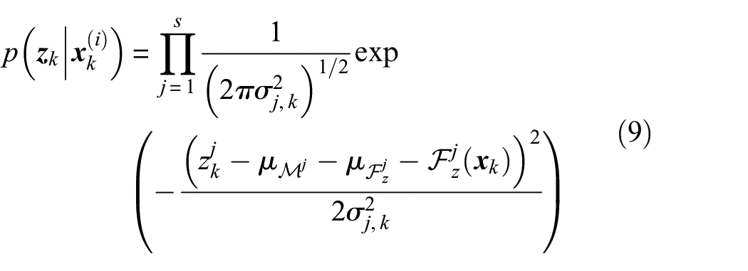
Replacing the model $M$ with the collection of $s$ surrogate models $F_{z}$ , with $F_{z} = [F_{z}^{1}, \dots, F_{z}^{j}, \dots, F_{z}^{s}]^{T}$ , requires the error function variance $σ_{j, k}^{2}$ in equation (7) to be updated, accounting also for the surrogate models error $n_{F_{z}} = [n_{F_{z}^{1}}, \dots, n_{F_{z}^{j}}, \dots, n_{F_{z}^{s}}]^{T}$ , where $n_{F_{z}^{j}}$ is the error related to the jth surrogate model prediction $F_{z}^{j} (x_{k})$ . Indeed, recalling equation (6), we can write the measurement equation as

z_{k} = F_{z} (x_{k}) + n_{F_{z}} + n_{M} + η_{k}

(8)

where it is made clear that $M (x_{k}) = F_{z} (x_{k}) + n_{F_{z}}$ . The error $n_{F_{z}}$ is assumed to be independent of the system state; furthermore, we assume that its probability distribution is Gaussian, that is, $n_{F_{z}} ~ N (μ_{F_{z}}, Σ_{F_{z}})$ , where the covariance matrix $Σ_{F_{z}}$ is diagonal due to the independency of the $n_{F_{z}}$ elements. We can thus easily derive the variance of the random variable constituted by the summation of the error terms, that is, $n = n_{F_{z}} + n_{M} + η_{k}$ , where $n ~ N (μ_{M} + μ_{F_{z}}, σ_{η, k}^{2} I + Σ_{M} + Σ_{F_{z}})$ . The resulting covariance matrix is still diagonal allowing to write equation (7) in its final form

\begin{matrix} p (z_{k} | x_{k}^{(i)}) = Π_{j = 1}^{s} \frac{1}{{(2 π σ_{j, k}^{2})}^{1 / 2}} \exp \\ (- \frac{{(z_{k}^{j} - μ_{M^{j}} - μ_{F_{z}^{j}} - F_{z}^{j} (x_{k}))}^{2}}{2 σ_{j, k}^{2}}) \end{matrix}

(9)

where the model $M$ has been replaced with the collection of $s$ surrogate models $F_{z}$ . The variance $σ_{j, k}^{2}$ is the jth entry of the resultant covariance matrix $σ_{η, k}^{2} I + Σ_{M} + Σ_{F_{z}}$ , while $μ_{F_{z}^{j}}$ is the jth entry of the vector $μ_{F_{z}}$ .

A thorough explanation on how the error terms distribution parameters are computed is provided in section ‘PF implementation’.

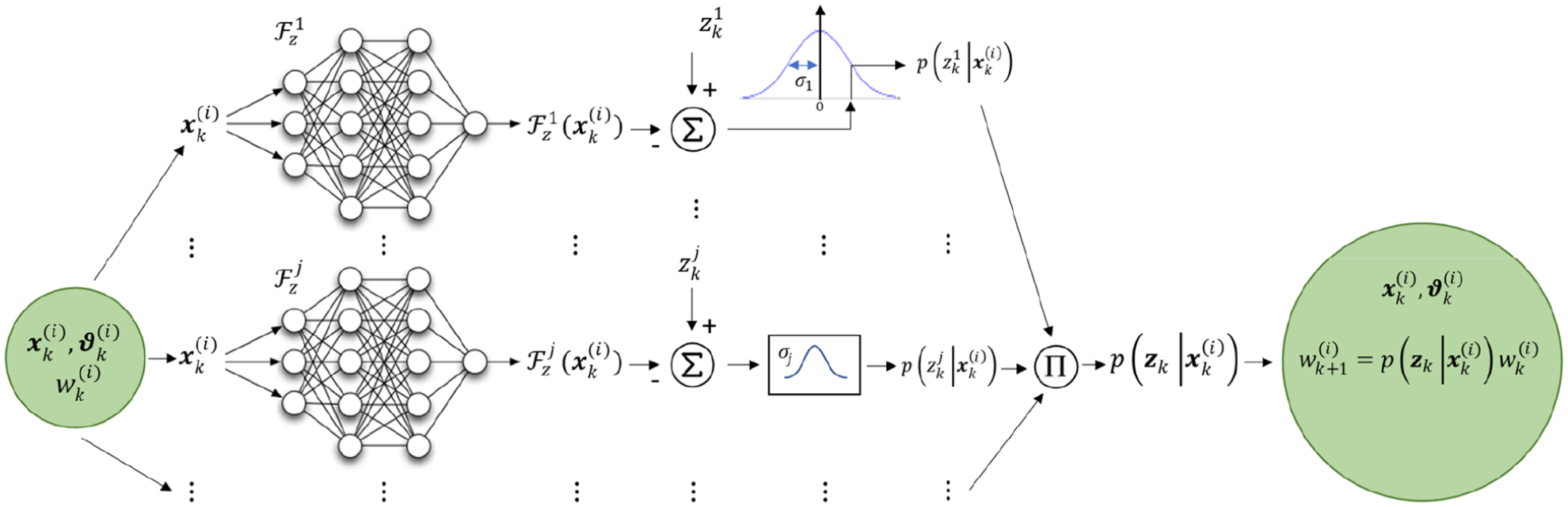
The procedure for the weight updating of samples (particles) is schematically summarized in Figure 1, where the process in equation (9) is broken down into a diagram showing the surrogate models $F_{z}^{j}$ role. The system state corresponding to the ith sample $x_{k}^{(i)}$ is fed to each one of the $s$ surrogate models; the jth surrogate model $F_{z}^{j}$ returns the system response estimate at the corresponding jth sensor location, that is, $F_{z}^{j} (x_{k}^{(i)})$ . The estimate $F_{z}^{j} (x_{k}^{(i)})$ is then compared to the jth sensor measurement $z_{k}^{j}$ , and the discrepancy $z_{k}^{j} - F_{z}^{j} (x_{k}^{(i)})$ is rated via an error function which indicates the likelihood of the state sample $x_{k}^{(i)}$ with respect to the measurement of the jth sensor $z_{k}^{j}$ , that is, $p (z_{k}^{j} | x_{k}^{(i)})$ ; the higher the discrepancy, the lower the likelihood of the state sample. The likelihood of the state sample with respect to the entire sensor network is then gathered as the product of the $s$ likelihoods, providing the sample unnormalized weigh updating factor $p (z_{k} | x_{k}^{(i)})$ .

Figure 1.

Surrogate modelling–based likelihood assessment scheme.

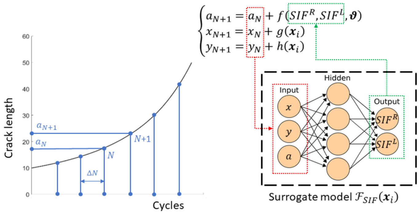
Another problem the PF algorithm may encounter is the projection of the particles trajectories ahead in time for the RUL estimate. The issue arises from the fact that the evolution model driving term, that is, SIF $Δ K$ in equation (10), is state dependent ( $SIF = f (x)$ ) and this dependency is not usually available in a closed form. Again, one might think of using the FEM $M$ , but this would lead to the computational burden pitfall. Notice that at the kth time index the single particle RUL estimate requires that the $SIF$ is simulated as many times as the number of increments the RUL has been segmented into for the crack numerical integration,³⁵ usually leading to an unmanageable number of simulations. Thus, following the same approach as before, we build an SIF ANN surrogate relating the state-space domain $D_{x} \subseteq R^{n_{s}}$ with the space of the SIFs $D_{SIF} \subseteq R^{2}$ , that is, $F_{SIF} : R^{n_{s}} \to R^{2}$ . The training data set for $F_{SIF}$ can benefit from the same database which has been generated for the training of the strain estimating surrogate models $F_{z}^{j}$ . The training data set for $F_{SIF}$ is the subset comprising the $S_{M} \times n_{s}$ input matrix $X$ and the $S_{M} \times 2$ output sub-matrix $Φ$ (note that, in general, the two crack tips are characterized by two different SIFs). A thorough description of the training process and ANN architecture is provided in the dedicated section.

Application to FCG

The deterministic degradation model

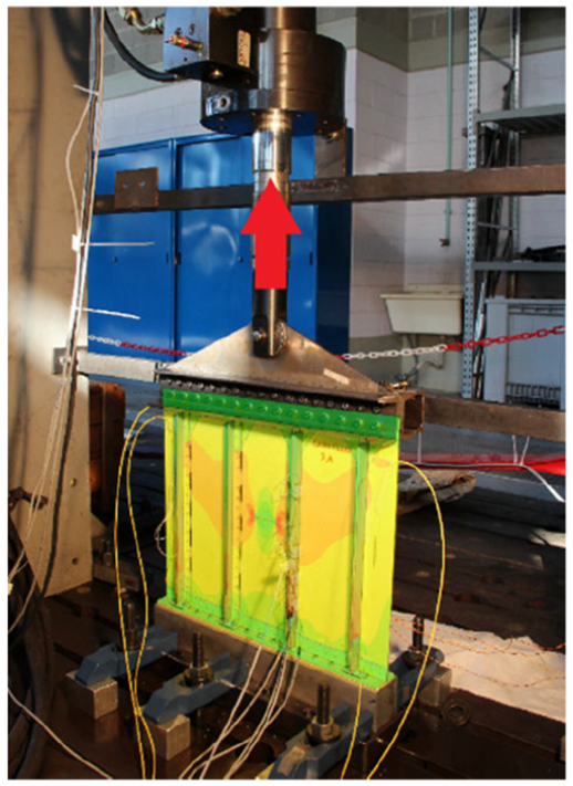
In this study, a realistic structure consisting of an aluminium alloy stiffened panel, replicating a sample of the rear fuselage of a medium–heavy weight helicopter (Figures 2 and 3), is considered. The panel specimen is constituted of a skin stiffened with four riveted stringers and some additional reinforcements in the upper and lower edges regions, specifically designed to obtain a stress field consistent with that experienced by the real structure, by distributing the applied load along the whole specimen width. The skin is made of Al2024T6 alloy, being 600 mm wide, 500 mm tall and 0.81 mm thick. The four L-shaped stringers are made of Al7075-T76 alloy, being 435 mm long and 1.2 mm thick and evenly spaced over the specimen skin surface.

Figure 2.

Fatigue testing facilities and specimen test setup.

Figure 3.

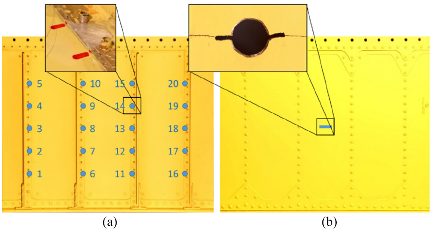
(a) Front and (b) rear view of the stiffened panel specimen. FBG strain gauges are installed on the stringers, in between rivets, after primer removal. A cut is machined at the middle of the central bay to initiate FCG.

The stiffened panel specimen is provided with an artificial notch located in the middle of the central skin bay, as illustrated in Figure 3(b), in a way that the fatigue crack initiation is favoured. This sort of damage can be considered representative of a generic impact causing a defect with subsequent nucleation of a skin crack and is also adopted for damage tolerance certification.¹ The specimen is subjected to constant amplitude sinusoidal loading along the stringers length direction (Figure 1), being characterized by 12-Hz frequency, 35-kN peak load and 0.1 load ratio $R$ , that is, the ratio between the minimum and the maximum load values within one load cycle. The panel is equipped with a network of $s = 20$ fibre Bragg grating (FBG) strain gauges located on the stringers as shown in Figure 3(a) and measuring the strain along their length direction. Sensor layout has been defined based on practical considerations and previous experience by the authors, in view of a real on-board application. Also, stringer strain field displays adequate sensitivity to changes in the skin panel, such as cracks propagating in the bay, allowing the degradation state identification.

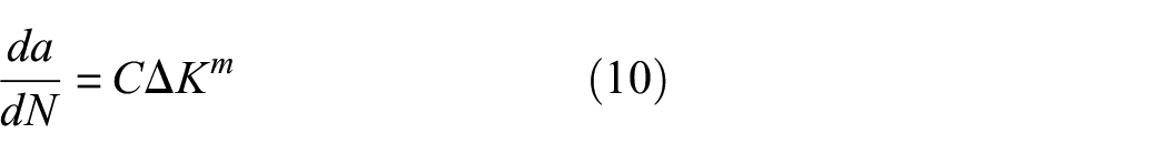
Although in our test case $R \neq 0$ , for simplicity, the state equation in equation (1) is chosen to be the Paris’ model,²⁵ where only the stable FCG phase will be considered, that is, the Paris’ region or region II in the FCG rate versus $Δ K$ (SIF range) curve

\frac{da}{dN} = C Δ K^{m}

(10)

where the left side represents the increase in the semi-crack length per cycle (FCG rate) and $Δ K = K_{\max} - K_{\min}$ is the SIF range within a loading cycle. The parameters $C$ and $m$ are usually obtained by fitting the curve to experimental data or found in the literature.

Equation (10) can be solved analytically only in a few simple cases, for instance, infinite plate with crack under mode I loading, where the crack location has practically no influence on the SIFs; in real case scenarios, one has to pursue the numerical integration route. Note that the crack state variables are the following: $x = {[x, y, a]}^{T}$ , where $x$ and $y$ are the crack centre coordinates and $a$ is the semi-crack length. If the crack state variable dependencies in equation (10) are made explicit, it is possible to obtain the following form: $\overset{\cdot}{a} = f (x, y, a)$ , which shows that the FCG rate is a function of the crack state variables only. The aim is to predict the crack length one-time increment (i.e. one load cycle) ahead, that is, at time $N + 1$ , given that the crack state variables at current time $N$ are known.

The simplest numerical integration method addressing the current problem is the explicit forward Euler method, where a linear approximation is being made across time increments, thus resulting in the following relation: $a_{N + 1} = a_{N} + f (x_{N}) Δ N$ , where $f (x_{N}) = {da / dN |}_{N}$ . In practice, equation (10) is rearranged into the following format

a_{N + 1} = a_{N} + C {(Δ K_{N})}^{m} Δ N

(11)

Note that the parameters $C$ and $m$ are independent of the index $N$ , while the SIF varies with $N$ . Also note that the assumption which is inherent to equation (11) is that the SIF is constant across the time increment $Δ N$ ; this, combined with the monotonic behaviour of the a–N curve, leads to an under estimation of the semi-crack length. To increase the accuracy of the prediction, $Δ N$ is set to unity in this work. For the sake of clarity, the SIF subscript will be omitted.

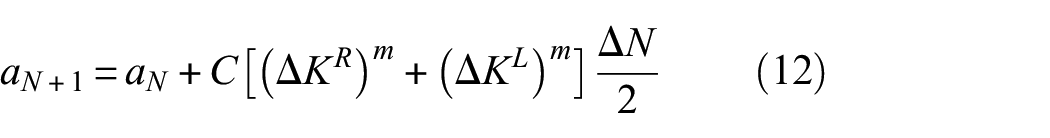
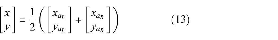
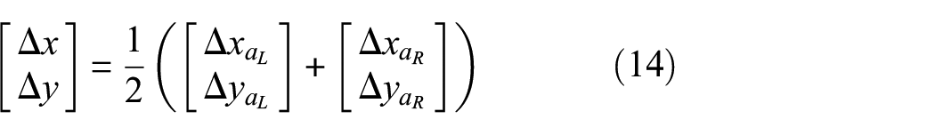
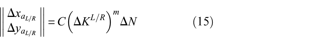
When considering a crack in a generic location of the bay, the stress field symmetry assumption might no longer be verified; the crack tips might be featured by different SIFs and crack propagation should contemplate them separately; as a consequence, the primary state space $x = [x, y, a]^{T}$ should be augmented with an additional variable: $x = [x, y, a_{R}, a_{L}]^{T}$ , where $a_{R}$ defines the right-hand side semi-crack length, while $a_{L}$ refers to the left-hand side. Therefore, two equations in the form of equation (11) are needed to describe the crack propagation, one for each crack tip. However, the FCG laws usually require the semi-crack length, meaning that the asymmetrical splitting of the crack makes little sense. Therefore, we manipulate the problem to get back to the original state-space variables, by simply considering an averaged semi-crack length

a_{N + 1} = a_{N} + C [{(Δ K^{R})}^{m} + {(Δ K^{L})}^{m}] \frac{Δ N}{2}

(12)

where $Δ K^{R}$ refers to the right-hand side SIF, while $Δ K^{L}$ refers to the left-hand one.

The crack centre location with respect to the updated crack tips can be expressed in a vector format as

[\begin{matrix} x \\ y \end{matrix}] = \frac{1}{2} ([\begin{matrix} x_{a_{L}} \\ y_{a_{L}} \end{matrix}] + [\begin{matrix} x_{a_{R}} \\ y_{a_{R}} \end{matrix}])

(13)

where $[\begin{matrix} x \\ y \end{matrix}]$ represents the crack centre location, while $[\begin{matrix} x_{a_{L}} \\ y_{a_{L}} \end{matrix}]$ and $[\begin{matrix} x_{a_{R}} \\ y_{a_{R}} \end{matrix}]$ refer to the left- and right-hand side crack tip positions, respectively.

The crack centre displacement across two subsequent observations can be quantified as follows:

[\begin{matrix} Δ x \\ Δ y \end{matrix}] = \frac{1}{2} ([\begin{matrix} Δ x_{a_{L}} \\ Δ y_{a_{L}} \end{matrix}] + [\begin{matrix} Δ x_{a_{R}} \\ Δ y_{a_{R}} \end{matrix}])

(14)

where $[\begin{matrix} Δ x_{a_{L / R}} \\ Δ y_{a_{L / R}} \end{matrix}]$ is the increase in the crack length between two consecutive observations at the left/right-hand side crack tip. The relation between these vector format quantities and the quantities in equation (12) is as follows

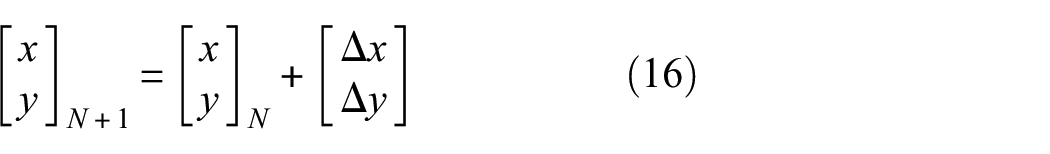
‖ \begin{matrix} Δ x_{a_{L / R}} \\ Δ y_{a_{L / R}} \end{matrix} ‖ = C {(Δ K^{L / R})}^{m} Δ N

(15)

The crack centre position evolution in time can be written as follows

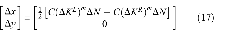
{[\begin{matrix} x \\ y \end{matrix}]}_{N + 1} = {[\begin{matrix} x \\ y \end{matrix}]}_{N} + [\begin{matrix} Δ x \\ Δ y \end{matrix}]

(16)

In Figure 4, the updating scheme described above is shown based on SIFs surrogate models. The equations written above are valid over a wide range of applications; indeed, the established framework can deal with a crack located anywhere in the bay and propagating along an inclined straight line. However, cracks loaded in mixed mode tend to propagate in mode I, meaning that, according to the present specimen features, a crack nucleating in the bay tends to propagate horizontally (observed experimentally). When the central crack scenario, prescribed by Department of USA Defense,¹ is analyzed, the following simplifying assumptions can be made: (a) due to the specimen symmetry with respect to a vertical plane passing through the central bay middle section, the stress field turns out to be symmetric; (b) due to the stress field symmetry with respect to the artificial notch, the crack is assumed to develop symmetrically; and (c) the crack position states are redundant in the prognostic stage, since the crack centre is assumed not to move. Based on these considerations, it is possible to write a simplified version of equations (13)–(16). Indeed, if the crack only propagates straight and horizontally, the crack centre coordinates can be updated as follows

[\begin{matrix} Δ x \\ Δ y \end{matrix}] = [\begin{matrix} \frac{1}{2} [C {(Δ K^{L})}^{m} Δ N - C {(Δ K^{R})}^{m} Δ N] \\ 0 \end{matrix}]

(17)

where, as expected, the state $y$ does not play any role. Equation (17) is referred to the panel specimen reference system, where the x–y plane lies on the skin plane, and the x-axis is horizontal and pointing towards the right-hand panel edge when looking from the stringers face side (Figure 5).

Figure 4.

Surrogate modelling–based FCG simulation according to forward Euler method of integration.

Figure 5.

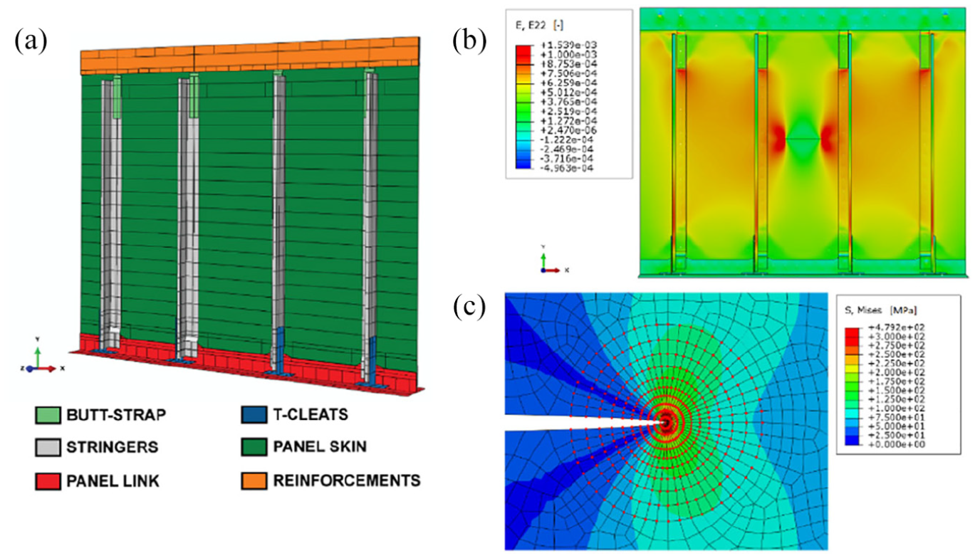
(a) High-fidelity model of the stiffened panel, (b) the presence of a skin crack is highlighted by the strain contour plot and (c) optimized mesh pattern for SIF calculation at the crack tip.

The high-fidelity model and the training data set

The high-fidelity model of the panel specimen consists of an FEM, built with the ABAQUS^® 6.14-5 software, establishing a relationship between the state-space vector $x$ and the specimen strain field (Figure 5), under the application of some axial load. Both stringers and skin were modelled with quadratic shell elements (S9R5), while rivets were represented as preloaded springs with proper stiffness values. The boundary conditions were opportunely chosen to replicate the experimental fixtures, as shown in Figure 2. More specifically, the load is applied to the specimen top edge, while the specimen bottom edge is clamped to ground through the lower panel link. Both specimen top and bottom edges are reinforced so that the load is uniformly distributed along the whole panel width. Crack damage was modelled with the SEAM command in ABAQUS, duplicating nodes at the two sides of the crack edge and allowing mode I crack opening.

The FEM has been optimized and validated in a previous work by the authors,³⁸ comparing the strain observations at sensors locations in presence of a crack damage with the simulated strain field values. To refine SIF calculations, an array of singular elements following the stress field singularity at the crack tip has been used (Figure 5(c)).

An example of the strain field sensitivity to skin damage is shown in Figure 5(b), as highlighted by the strain contour plot. When a skin crack grows, it causes a modification of the load paths within the skin, increasing the load carried by stringers. This load transfer effect is higher in the proximity of the crack so that, if a sufficient number of sensors is adopted, strain field features can be adopted to identify damage characteristics (i.e. crack centre coordinates $[x, y]$ and semi-crack length $a$ ) based on strain observations. In the Bayesian framework described in section ‘Theoretical background’, this translates in setting $n_{s} = 3$ state variables to be identified based on $s = 20$ strain observations.

The FEM has thus been parametrised in terms of crack centre coordinates and semi-crack length, and a combination of MATLAB^® and Python scripts has been used to generate a database of strain patterns relative to 1700 damage cases, increased to $S_{M} = 3400$ , if the symmetry with respect to the vertical plane is taken into account. In particular, 17 crack lengths have been simulated, ranging from 20 to 100 mm, with a 5-mm step. The maximum crack length (100 mm) is defined based on practical considerations; thus, the EoL or end of prediction (EoP) is reached as soon as the crack length reaches 100 mm. A total of 100 crack centre positions have been considered for each crack length, randomly sampling the $[x, y]$ coordinates of the crack centre within the skin area to favour a more homogeneous scanning of the state-space domain $D_{x}$ . The strain pattern at $s = 20$ sensor positions and the SIFs at the two crack tips have been calculated for each case.

Surrogate models for strain estimates

Intending to alleviate the computational burden associated with the high-fidelity models being run several times, a set of strain-predicting surrogate models has been exploited, taking advantage of the power of multilayer perceptron (MLP) ANNs. We recall here that a bank of $s$ surrogate models $F_{z}^{j}$ , $j = 1, \dots, s$ , based on $s$ MLP ANNs, is used in place of the original FEM $M$ , as described in section ‘Theoretical background’, whereas the burdensome model $M$ is exploited offline to build the corresponding training data sets $T_{j} = {X; E_{j}} = {x_{i}; ε_{i}^{S_{j}}}_{i = 1}^{S_{M}}$ , where $j = 1, \dots, s$ and $ε_{i}^{S_{j}} = M^{j} (x_{i})$ , letting $M^{j} (x_{i})$ represents the jth element of the response vector $M (x_{i})$ . Each training data set comprises an $S_{M} \times n_{s}$ input matrix $X$ and an $S_{M} \times 1$ output vector $E_{j}$ ; note that all training data sets share the same input matrix $X$ . The input matrix ith row $x_{i} = [x_{i}, y_{i}, a_{i}]$ features the ith degradation state sample, while the output vector $E_{j}$ ith element shows the jth sensor strain prediction for the ith degradation state sample $x_{i}$ , that is, $ε_{i}^{S_{j}} = M^{j} (x_{i})$ , so that

X = [\begin{matrix} x_{1} \\ ⋮ \\ x_{S_{M}} \end{matrix}]; E_{j} = [\begin{matrix} ε_{1}^{S_{j}} \\ ⋮ \\ ε_{S_{M}}^{S_{j}} \end{matrix}]

(18)

Note that the system measured response is here denoted with the letter $ε$ instead of $z$ to emphasize its nature; the two notations are interchangeable. Thus, after training, when fed with a new degradation state sample $x_{*} \notin T_{j}$ , each surrogate model shall predict the strain for the corresponding sensor, that is, ${\hat{z}}^{j} = F_{z}^{j} (x_{*})$ , so that $F_{z}^{j} (x_{*}) \approx M^{j} (x_{*})$ . The MATLAB Deep Learning Toolbox™ has been used for the implementation of the ANN surrogate models. Specifically, the Neural Fitting app (‘nftool’) has been employed along this work.

The ANN architecture is made up of a three neuron input layer, a 70 neuron hidden layer and a single neuron output layer; the first layer activation function is a hyperbolic tangent ( $f^{1}$ ), whereas the second-layer activation function is linear $(f^{2})$ . The representative equation of the jth ANN is shown in equation (19), where the weights are collected in the matrices $W$ and the biases in the vectors $b$

\hat{z} = f^{2} (W_{2, 1} f^{1} (W_{1, 1} x + b_{1}) + b_{2})

(19)

Note that all the $s$ ANNs share the same architecture; the number of hidden neurons has been selected by testing the accuracy of the predictions with varying the hidden layer size for a subset of randomly selected sensors and then selecting the size providing the overall highest accuracy, that is, 70 hidden neurons. The loss function ruling the backpropagation is the mean square error (MSE). Quasi-Newton optimization algorithm is selected for the weights and biases updating. To improve generalization, early stopping is adopted, where training data are divided into three subsets. The first subset is the training subset (used for computing the gradient and for updating the weights). The second subset is the validation set, which is used to monitor overfitting. When the validation error consecutively rises for a specified number of iterations, training is stopped, and weights at the minimum of the validation error are kept. The test set is used to compare different models or to consolidate the validation set, spotting poor data set separation. Training, validation and test subsets feature a 70%–15%–15% proportions, respectively, stopping the training when the validation error increases for eight consecutive training epochs.

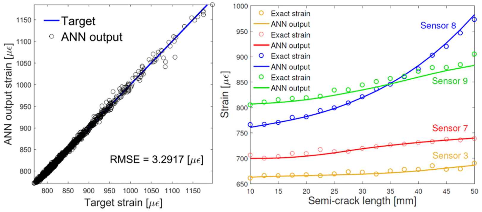
The strain prediction performances of the $j = 7$ ANN are shown in Figure 6 (left), where the regression plot between target and predicted strains refers to a test set not included in the training set, and made up of cracks with different lengths randomly spread over the area enclosed by the sensors grid. The strain sensitivity of sensor IDs 3, 7, 8, and 9 to a propagating crack centred in the middle bay is illustrated in Figure 6 (right), which also shows the ANNs prediction errors.

Figure 6.

Regression plot for ANN performance assessment under a test data set (left); strain sensitivity for sensor IDs 3, 7, 8, 9 (right).

Surrogate models for SIF prediction

The SIFs surrogate model leverages again on an MLP ANN, given the same $S_{M} \times n_{s}$ input matrix $X$ and the $S_{M} \times 2$ output matrix $Φ$ comprising the crack SIFs (left and right). Therefore, the output matrix ith row, $ϕ_{i} = [{SIF}_{i}^{R}, {SIF}_{i}^{L}]$ comprises the right and left-hand side SIFs for each crack state sample $x_{i}$ . The ANN for the SIFs estimates relies on the same architecture of the ANNs used for the strain prediction, except the output layer, which has two neurons.

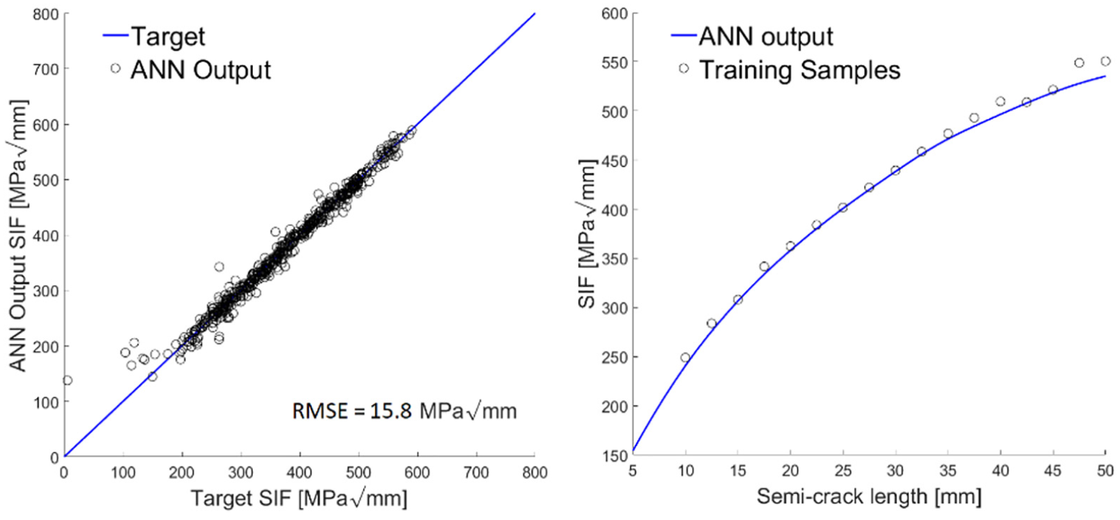
The training performance of the surrogate model is shown in Figure 7 (left), obtained with the same procedure used for Figure 6. The SIF sensitivity to a propagating crack centred in the middle bay is illustrated in Figure 7 (right), along with prediction errors.

Figure 7.

Regression plot for ANN performance assessment under a test data set (left); SIF sensitivity with respect to crack size – centre bay crack is used – (right). Note that the left and right SIFs are equal due to the crack centre position.

PF implementation

The proposed PF algorithm is an SIR with systematic resampling.³⁹ The PF tasks are (1) estimating the system degradation states, that is, the fatigue crack location ( $x, y$ ) and size ( $a$ ) collected in $x$ and (2) predicting the degradation evolution and the panel specimen RUL, on the basis of indirect time-spaced observations of the hidden degradation state variables. This last task implies the identification of the degradation model parameters ( $C$ and $m$ ), which, due to the inter-specimen variability, are not known a priori, thus motivating the augmented state formulation ( $y_{k} = [x_{k}, ϑ_{k}]^{T}$ ).³⁷ This strategy provides additional flexibility to the PF, allowing to capture more complicated dynamics, for example, variable load ratio, without the need of more sophisticated degradation models.^40,41

The RUL is computed based on the EoP, which coincides here with a crack length of 100 mm, independently of the crack centre location; from now on, the EoL will be used in place of the EoP.

The PF predictive stage is described by the evolution function reported in equation (1), which requires the transition density function of the state variables, $p (x_{k} | x_{k - 1}, ϑ_{k - 1})$ , as well as the transition density function of the parameters ruling the deterministic degradation model, $p (ϑ_{k} | ϑ_{k - 1})$ . The transition kernel $p (x_{k} | x_{k - 1}, ϑ_{k - 1})$ , given the parameters $ϑ_{k - 1} = [C_{k - 1}, m_{k - 1}]^{T}$ , is obtained by adding to the degradation model states the process noise $u_{k} = [v_{k}, q_{k}]^{T}$ , which accounts for the inherent stochasticity of the degradation process. Equations (12), (16) and (17) describe the state variables $x = [x, y, a]^{T}$ deterministic evolution in time: the averaged semi-crack size prediction across two subsequent inspection times is unveiled in equation (12), while the crack centre coordinates updating is described in equations (16) and (17). The crack state variables vector $x$ is split in a way that the crack centre coordinates are merged, that is, $x = [c, a]^{T}$ , since variables are treated differently when performing the transition from deterministic to stochastic evolution models. A log-normal distribution is selected for the process noise $q_{k}, q_{k} ~ e^{N (- σ_{q}^{2} / 2, σ_{q}^{2})}$ , polluting the crack size growth equation; the log-normal distribution assures that $q_{k}$ is always positive, while the normal distribution mean value, that is, $- σ_{q}^{2} / 2$ , makes sure that the crack size projection in time is non-biased⁴²

a_{k}^{(i)} = f (x_{k - 1}^{(i)}, ϑ_{k - 1}^{(i)}) \cdot q_{k}

(20)

where the function $f$ is representing the deterministic degradation model in equation (12). The process noise components affecting the crack centre coordinates are collected in the vector $v_{k}$ , where $v_{k}$ is sampled from $N (0, d \cdot Σ [c]_{k - 1})$ , where $Σ [c]_{k - 1}$ is the covariance matrix of the collection of coordinate samples at the previous step ( $c = [x, y]^{T}$ ). This approach allows the noise variance to reduce as far as the particles cluster around the true crack centre position, at the expense of an additional parameter $d$ weighting the covariance matrix. Therefore, the crack centre evolution in time is driven by the following equation

c_{k}^{(i)} = t (x_{k - 1}^{(i)}, ϑ_{k - 1}^{(i)}) + v_{k}

(21)

where the function $t$ is representing the deterministic model governing the crack centre coordinates stated in equation (17). The transition density function of the parameters, $p (ϑ_{k} | ϑ_{k - 1})$ , which drives the generation of new particles samples $ϑ_{k}^{(i)}$ , is based on a Kernel smoothing approach³⁷

ϑ_{k}^{(i)} = \sqrt{1 - h^{2}} ϑ_{k - 1}^{(i)} + (1 - \sqrt{1 - h^{2}}) E [ϑ_{k - 1}] + r

(22)

where $r$ is sampled from $N (0, h^{2} \cdot Σ [ϑ]_{k - 1})$ , where $Σ [ϑ]_{k - 1}$ is the covariance matrix of $ϑ_{k - 1}$ , and $E [ϑ_{k - 1}]$ is the expected value of $ϑ$ computed at the previous step $k - 1$ .

The system state updating is driven by equation (9), which operates the likelihood assessment taking into consideration all the error sources affecting the measurement equation; these sources sum up into the cumulative error term $n$ , that is, $n = n_{F_{z}} + n_{M} + η_{k}$ , where $n ~ N (μ_{M} + μ_{F_{z}}, σ_{η, k}^{2} I + Σ_{M} + Σ_{F_{z}})$ . We recall that the measurement noise $η_{k}$ is zero-mean normally distributed, and its components are independent and identically distributed (i.i.d.), that is, $η_{k} ~ N (0, σ_{η, k}^{2} I)$ , where $I$ is the identity matrix. Note that the observation noise variance has been derived by analysing samples of the measurements during the experimental activities (the noise level can also be inferred during operation); since no significant noise level variations have been observed in time, the time dependency is cancelled out, that is, $η ~ N (0, σ_{η}^{2} I)$ .

The jth surrogate model prediction error $n_{F_{z}^{j}}$ distribution is inferred fitting the test-set error histogram with a normal pdf, that is, $n_{F_{z}^{j}} ~ N (μ_{F_{z}^{j}}, σ_{F_{z}^{j}}^{2})$ , with $j = 1, \dots, s$ . This method collapses the information relative to the state-space variables, that is, the error $n_{F_{z}^{j}}$ dependency on the state $x_{k}$ . In our study, the surrogate models biases $μ_{F_{z}^{j}}$ approach zero ( $\forall j = 1, \dots, s$ ), while their error variances $σ_{F_{z}^{j}}^{2}$ were comparable: the surrogate model error $n_{F_{z}}$ has a pdf which is similar to the one featuring the measurement noise $η$ , that is, $n_{F_{z}} ~ N (0, σ_{F_{z}}^{2} I)$ .

Recalling the relation elapsing between the approximated system response prediction $M (x_{k})$ and the ground truth represented by $g (x_{k})$ , that is, $g (x_{k}) = M (x_{k}) + n_{M}$ , it is clear that both $M (x_{k})$ and $g (x_{k})$ are needed to infer the pdf of $n_{M}$ . The response $g (x_{k})$ can be readily computed from equation (1), observing that the system measured response stands as $z_{k} ~ N (g (x_{k}), σ_{η}^{2} I)$ . Therefore, it is possible to compute $g (x_{k})$ as the expectation of a sufficiently large sample of the system response, that is, $g (x_{k}) = 1 / N \sum_{i}^{N} z_{k}^{i}$ , where $z_{k}^{i}$ is the ith sample of the system measured response. However, this would require that several experimental tests are run to check a representative sample of the state space, which is not feasible. Within this work, we assume that the error $n_{M}$ does not depend on the system state $x_{k}$ ; under this assumption, it is possible to estimate $n_{M}$ by testing the healthy structure and then comparing its response with the response predicted by the FEM, $n_{M} = g (x_{- 1}) - M (x_{- 1})$ , where $x_{- 1}$ indicates the healthy state. This approach makes $n_{M}$ deterministic: $n_{M} ~ N (μ_{M}, 0_{s, s})$ , where $μ_{M} = g (x_{- 1}) - M (x_{- 1})$ and $0_{s, s}$ indicates a null covariance matrix. It is worth mentioning that accounting for $n_{M}$ has the same effect as calibrating the FEM, since we are removing the model prediction bias.

Based on the above considerations, the cumulative error pdf is defined as follows $n ~ N (μ_{M}, Σ_{n})$ , where $Σ_{n} = (σ_{η}^{2} + σ_{F_{z}}^{2}) I$ . Therefore, equation (9) evolves into the following form

\begin{matrix} p (z_{k} | x_{k}^{(i)}) = \frac{1}{{(2 π σ^{2})}^{s / 2}} \exp \\ (- \frac{1}{2 σ^{2}} \sum_{j = 1}^{s} {(z_{k}^{j} - μ_{M^{j}} - F_{z}^{j} (x_{k}))}^{2}) \end{matrix}

(23)

where $σ = σ_{η}^{2} + σ_{F_{z}}^{2}$ is the jth entry of $Σ_{n}$ . It is worth noting that it is common practice to adopt a larger value for $σ^{2}$ to compensate for the increased uncertainty deriving from the assumption which are made about the error sources and to maintain sample variety.

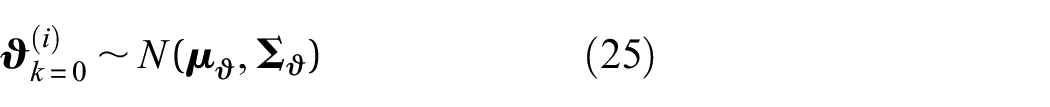
The PF algorithm has to be initialized based on any available prior information about the degradation state and the degradation model parameters, sampling the particles accordingly (Table 2). In the absence of any specific prior knowledge on the degradation state, we set the state variables prior distribution to be uniform, with bounds enclosing the physical domain of the problem, as stated in equation (24)

x_{k = 0}^{(i)} ~ U (a_{x}, b_{x}); y_{k = 0}^{(i)} ~ U (a_{y}, b_{y}); a_{k = 0}^{(i)} ~ U (a_{a}, b_{a})

(24)

Table 2.

The sequential importance resampling particle filters algorithm.

Sample

y_{1}^{(i)}

with

i = 1, \dots, N_{s}

according to equations (24) and (25)
For

k = 1 : N_{obs}

k = 1

Evaluate the likelihood

L_{1}^{(i)}

for each sample

y_{1}^{(i)} = [x_{1}^{(i)}, ϑ_{1}^{(i)}]

where

x_{1}^{(i)} = [a_{1}^{(i)}, x_{1}^{(i)}, y_{1}^{(i)}]

L_{1}^{(i)} = p (z_{1} | x_{1}^{(i)})

Assign weights to particles:

{\bar{w}}_{1}^{(i)} = L_{1}^{(i)}

Normalize particles weights:

w_{k}^{(i)} = \frac{{\bar{w}}_{k}^{(i)}}{\sum_{j = 1}^{N_{s}} {\bar{w}}_{k}^{(j)}}

Resample the particles based on their weights
Sample

ϑ_{1}^{(i)}

according to the bivariate normal

ϑ_{1}^{(i)} ~ N (μ_{ϑ}, σ_{ϑ}^{2})

k > 1

Project crack size

a_{k - 1}^{(i)}

one step ahead according to equation (20)
Update crack centre

[x_{k - 1}^{(i)}, y_{k - 1}^{(i)}]^{T}

according to equation (21)
Evaluate the likelihood

L_{k}^{(i)}

for each sample

y_{k}^{(i)} = [x_{k}^{(i)}, ϑ_{k}^{(i)}]

L_{k}^{(i)} = p (z_{k} | x_{k}^{(i)})

Update particles weights:

{\bar{w}}_{k}^{(i)} = w_{k - 1}^{(i)} L_{k}^{(i)}

Normalize particles weights:

w_{k}^{(i)} = \frac{{\bar{w}}_{k}^{(i)}}{\sum_{j = 1}^{N_{s}} {\bar{w}}_{k}^{(j)}}

Resample the particles based on their weights
Compute the remaining useful life for each particle:

{RUL}_{k}^{(i)} = {EoL}_{k}^{(i)} - N_{k}

Parameters updating:

ϑ_{k}^{(i)} = \sqrt{1 - h^{2}} ϑ_{k - 1}^{(i)} + (1 - \sqrt{1 - h^{2}}) E [ϑ_{k - 1}] + r

In real applications, a certain amount of prior knowledge might be available and can be exploited to define better priors and speeding the filtering process. $C$ and $m$ initializing mean values and associated uncertainties can be found in the literature. Here, prior relevant information about $C$ and $m$ distribution is gathered from the pioneering work of Virkler et al.²⁶ Note that $C$ and $m$ are not independent; it is therefore crucial to take into consideration their intrinsic correlation.^26,27,43 Specifically, a bivariate normal distribution is selected to represent their joint pdf

ϑ_{k = 0}^{(i)} ~ N (μ_{ϑ}, Σ_{ϑ})

(25)

PF benchmark scenario

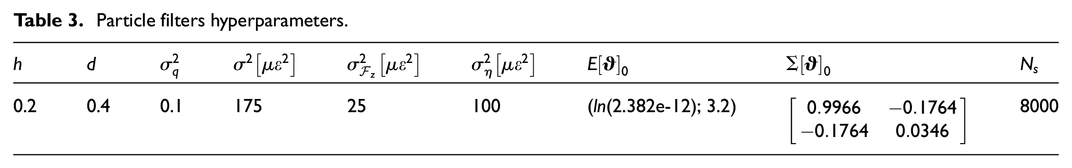
The proposed PF is first tested with a synthetic version of the middle-bay central-crack FCG scenario (FCG is symmetric). This scenario is described by an analytical–numerical hybrid approach, where the crack is iteratively propagated according to equation (11), while the SIF at the crack tip is updated according to a polynomial function relating the SIF to the crack size, which was made available by the NASA technical report repository.⁴⁴ Strain observations are numerically generated via the FEM described above, by simulating the strain field response in correspondence of discrete crack sizes, intentionally adopting a coarse increment size and then interpolating the resulting data points, to have continuous in time strain at the observation locations. Finally, strain observations are artificially polluted with zero-mean normally distributed measurement noise. The noise variance $σ_{η}^{2}$ is estimated analysing samples of the experimental measurement signals, yielding a value which is roughly 10 $μ ε^{2}$ . However, the value has been increased up to 100 $μ ε^{2}$ to simulate a heavily noisy environment. Variance associated with the surrogate model prediction error $σ_{F_{z}}^{2}$ is approximately equal to 25 $μ ε^{2}$ . The likelihood function variance $σ^{2}$ has been set to 175 $μ ε^{2}$ , with a 40% increase over its lower bound value of 125 $μ ε^{2}$ . It is worth mentioning that within this simulated scenario the error term $n_{M}$ associated with the FEM $M$ is clearly null. The PF hyperparameters are shown in Table 3.

Table 3.

Particle filters hyperparameters.

$h$	$d$	$σ_{q}^{2}$	$σ^{2} [μ ε^{2}]$	$σ_{F_{z}}^{2} [μ ε^{2}]$	$σ_{η}^{2} [μ ε^{2}]$	$E {[ϑ]}_{0}$	$Σ {[ϑ]}_{0}$	$N_{s}$
0.2	0.4	0.1	175	25	100	( $\ln$ (2.382e-12); 3.2)	$[\begin{matrix} 0.9966 & - 0.1764 \\ - 0.1764 & 0.0346 \end{matrix}]$	8000

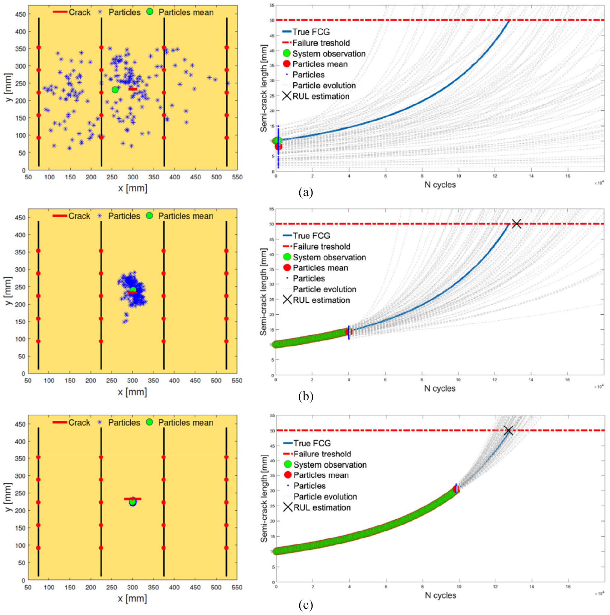
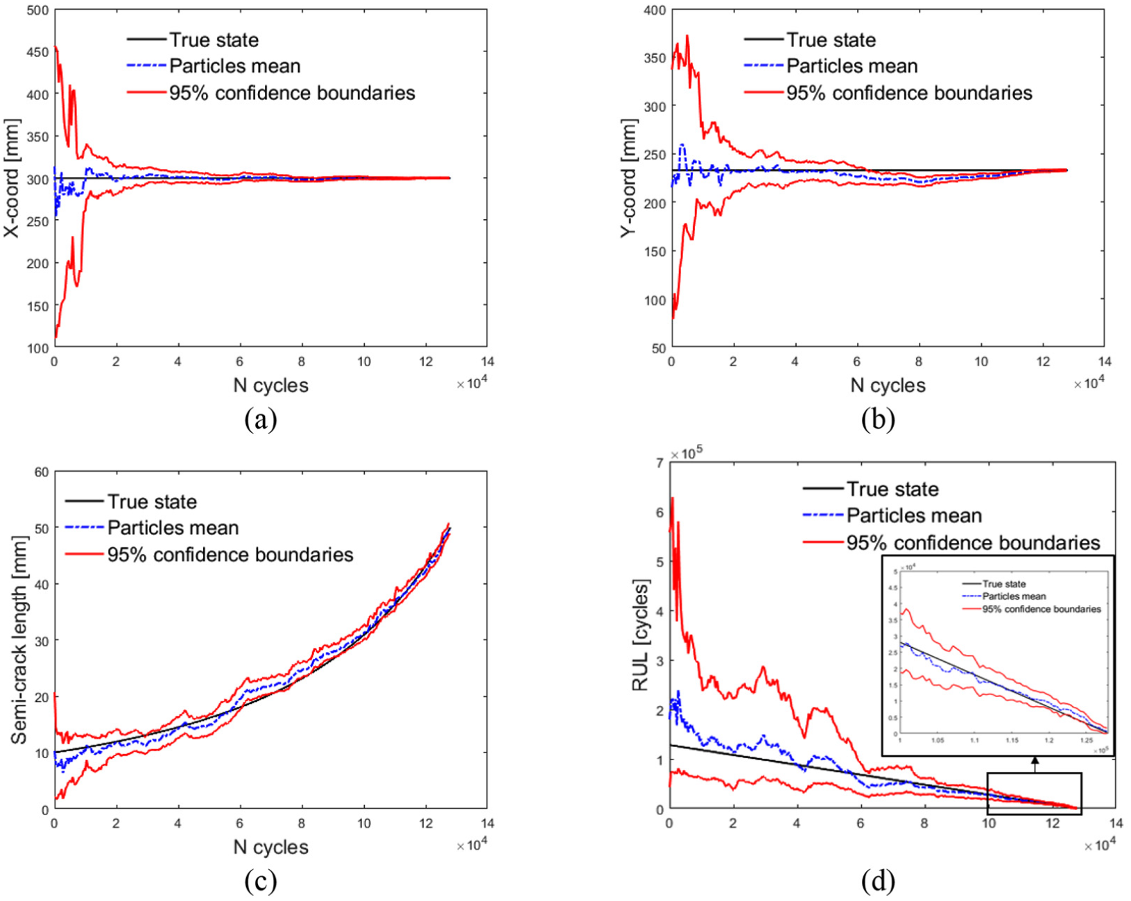
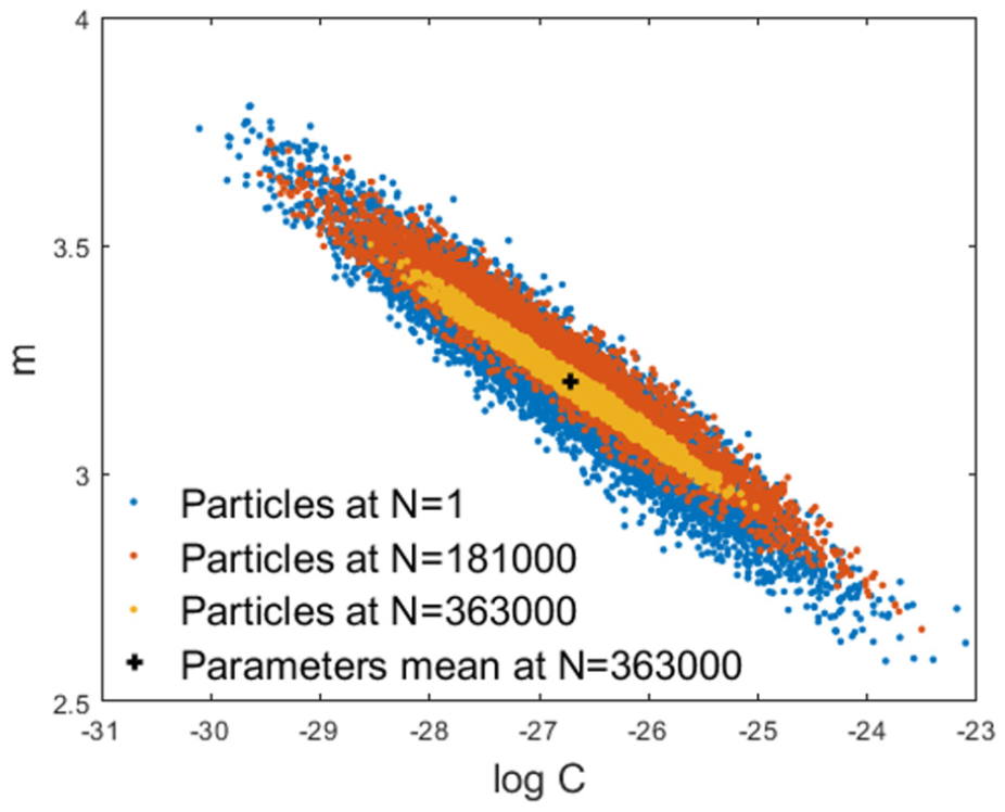
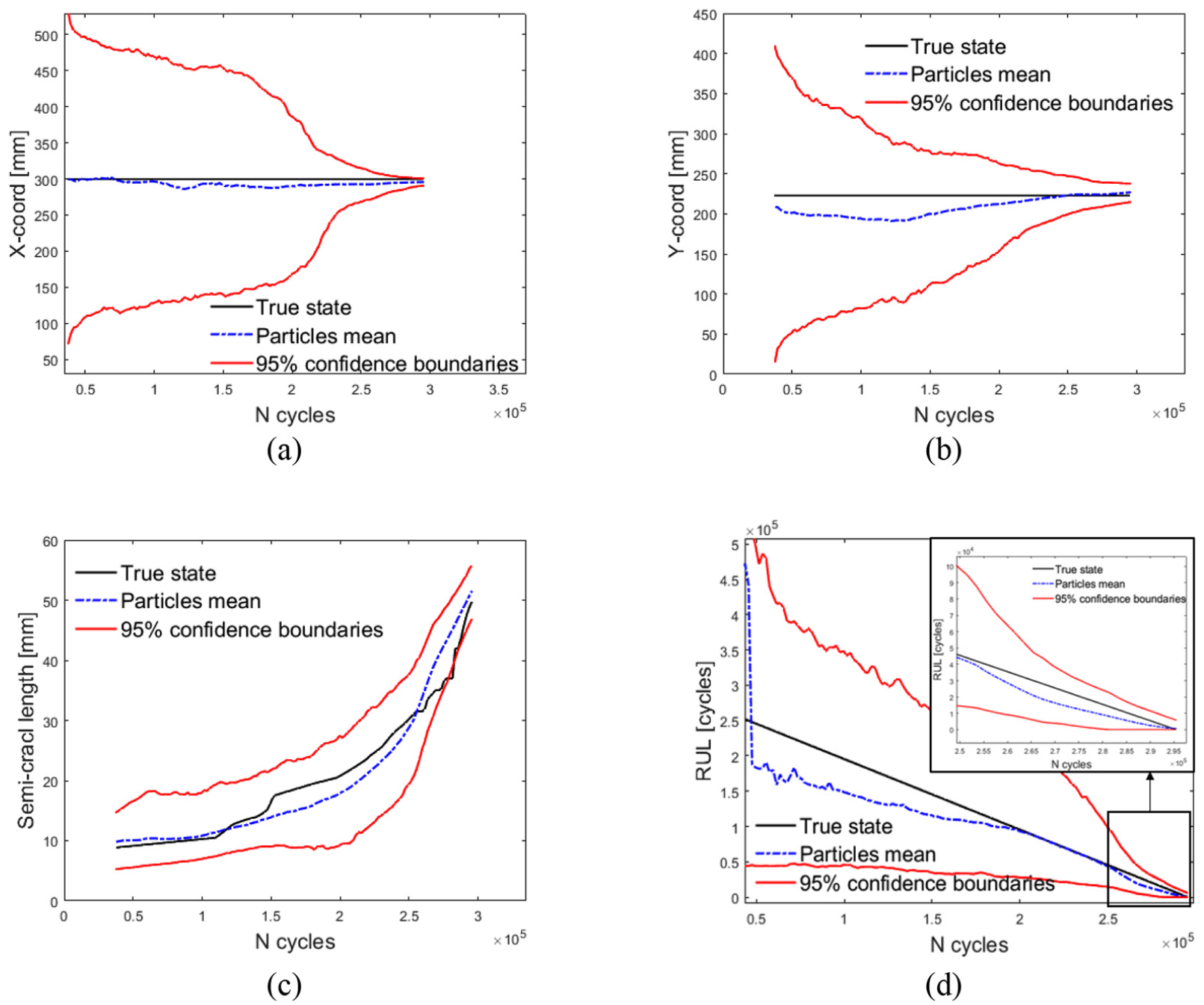
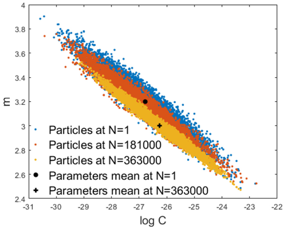
Figures 8 and 9 show the PF diagnostic and prognostic results; the particle state posterior pdf with respect to the benchmark scenario is shown; more specifically, Figure 8 shows the particles state variables distribution at different stages (number of load cycles) of the panel specimen life. It can be seen that the longer the stream of available observations, that is, $z_{1 : k - 1}$ , the lower the uncertainty affecting the knowledge about the degradation state and the parameters governing the dynamic behaviour. Figure 8(a) shows the state variables posterior pdf after one filtering stage and the corresponding particle trajectories projected into the future. Figure 8(b) and (c) shows a snapshot of the state variable posterior pdf after 40 and 100 observations, respectively. From a diagnostic point of view, one can observe that the cloud of particles tends to cluster around the true state as new observations are collected, whereas, from a prognostic point of view, the thickening of the particle trajectories about the reference FCG curve is seen to be dependent on the amount of available collected information in the form of observations. Consequently, the RUL prediction, that is, the mean of the posterior pdf of the particle RULs, approaches the true value as the number of available observations increases. The performances of the PF are shown in Figure 9, where one can assess the PF diagnostic performance in estimating the hidden degradation state variables, whereas the predictive performance in terms of system RUL is plotted in Figure 9(d). However, the prognostic performance is affected by the unknown evolution model parameters $ϑ_{k} = [C_{k}, m_{k}]^{T}$ , which are included in the augmented state vector $y_{k}$ . The parameter evolution, driven by a Kernel smoothing approach, is shown in Figure 10. Note that the distribution, which is initially a bivariate Normal, reduces its variance with increasing the number of observations, keeping a similar level of correlation and converging to the true parameter values.^26,27,43

Figure 8.

PF performance at different stages: (a) 1 observation, (b) 40 observations and (c) 100 observations.

Figure 9.

PF diagnostic and prognostic result as a function of time. (a)–(c) Diagnostic performance in the degradation states estimation as a function of time. (d) RUL estimates as a function of time.

Figure 10.

C and m parameters’ distribution at different observation times.

PF experimental data set scenario

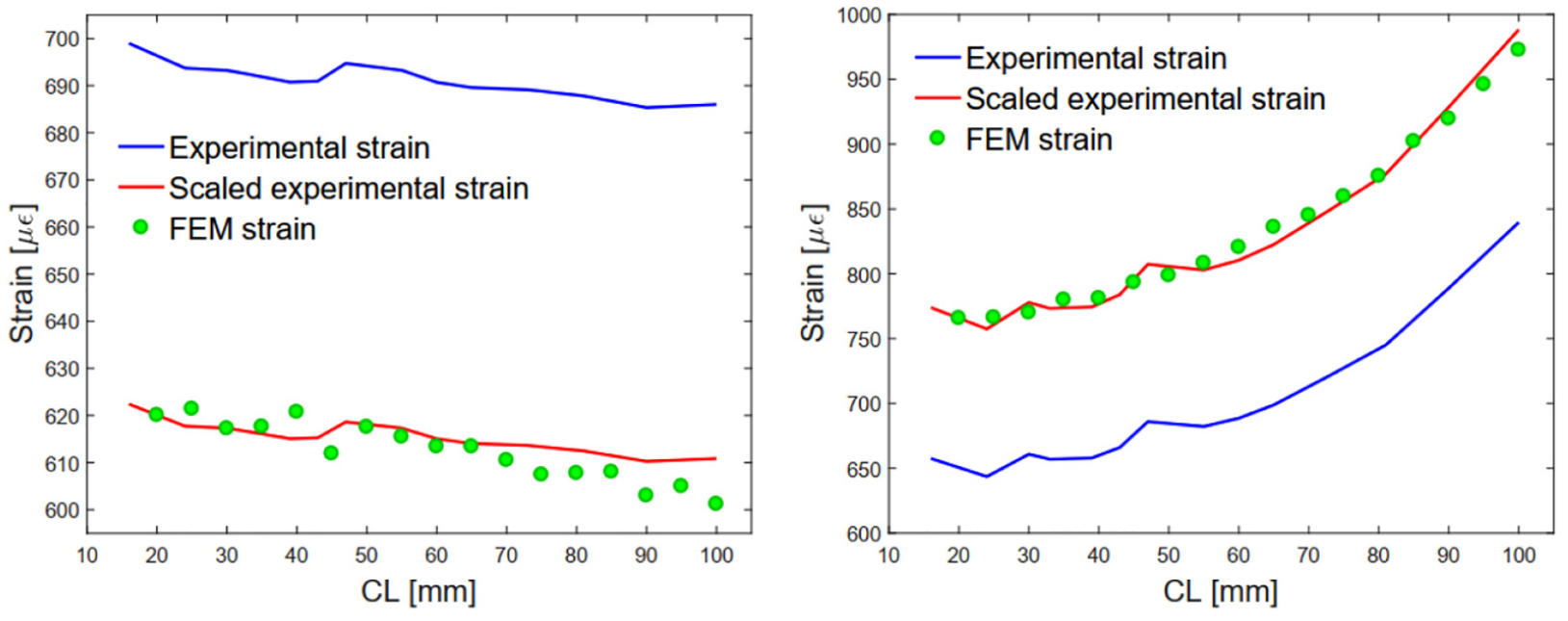
The experimental FCG tests have been performed on a batch of four identical panel specimens, collecting the sensor network strain measurements every 10³ loading cycles. The experimental data set PF shares the same hyperparameters used in the benchmark scenario (Table 3). However, the measurement noise level is substantially lower ( $σ_{η}^{2} = 10 μ ε^{2}$ ), while the error term $n_{M}$ associated with the FEM $M$ prediction of the system response has been accounted for by subtracting $n_{M}$ to the measured system response $z_{k}$ . The likelihood variance has been kept at the same value as in the simulated scenario, that is, 175 $μ ε^{2}$ . This substantial increase with respect to the lower bound value has been dictated by the fact that the error term $n_{M}$ has proved state dependent; evidence was uncovered by comparing the FEM prediction of the system response against the observed system response for the FCG scenario experimentally tested, as shown in Figure 11. Another reason prompting a considerable increase in the likelihood function variance lies in the uncertainty affecting FCG. Indeed, deviations from the expected trajectory (according to the evolution model) are to be expected; although the augmented state formulation addresses the issue, an increased likelihood function variance favours sample variety.

Figure 11.

FE model and experimental strain versus crack length (CL) error and scaling.

Figure 12 shows, for the sake of brevity, only the results related to one panel specimen. The differences between the experimental FCG and the simulated one are significant; for instance, the experimental RUL is almost three times the simulated one. In spite of the differences, the PF performances are satisfactory, always converging to the true degradation states. However, the RUL prediction (Figure 12(d)) seems to be more distant from the true state than in the simulated benchmark. The increased uncertainty of the PF state estimates with respect to the simulated scenario is substantial; this can be explained by recalling the fact that the error term related to the FEM prediction of the system response is not constant, as it is assumed (see Figure 11). The PF, via the augmented state formulation, demonstrates its ability in determining the parameters $C$ and $m$ which better describe the FCG, extending the Paris’ model validity out of the $R = 0$ boundary. Figure 13 shows the degradation model parameters ( $C, m$ ) at different observation times; as for the simulated scenario, the sample variances becomes smaller for an increasing number of observations, thickening around the values which make the FCG model closer to the experimental data.

Figure 12.

PF diagnostic and prognostic result as a function of time. (a)–(c) Diagnostic performance in the degradation states estimation as a function of time. (d) RUL estimates as a function of time.

Figure 13.

C and m parameters’ distribution at different observation times.

It is worth to examine the performance of the proposed framework in terms of analysis time, so that the ‘real-time’ requirement is quantitatively evaluated, providing evidence supporting the surrogate modelling strategy superiority over the high-fidelity FEM. To provide a fair comparison for the analysis time, all the computational tasks are implemented on a desktop PC equipped with a six-core 3.7 GHz Intel Core^™ i7-8700K processor. The PF analysis time required to process one set of observations ranges from 0.4 up to 1.8 s approximately, depending on how close is EoL to the current system crack length mean value; indeed, computing time strongly depends on the average RUL, since state samples need to be projected ahead in time up to EoL. By comparison, if we used the high-fidelity FEM in place of surrogate models of the same, the analysis time required to process one set of observations would be of a few days at best (supposing an FEM analysis of 15 s), due to the large number of simulation calls which are necessary.

The prognostic performances of the PF algorithm are measured by the following accepted metrics.

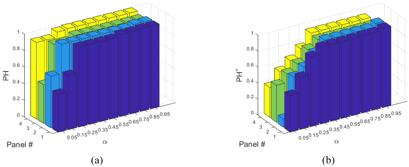
The prognostic horizon (PH) is the time elapsing between the first time $t_{k}^{*}$ the estimated RUL ( ${\bar{r}}_{k}$ ) enters a given band surrounding the ground truth RUL ( $r_{k}$ ) and the specimen end of life, that is, $EoL$ : $PH = EoL - t_{k}^{*}$ . Bandwidth amplitude $α$ is defined by the user as a $EoL$ percentage, mainly based on practical considerations tailored to the specific context. PH results are shown in Figure 14(a), where the prognostic metric is evaluated for each panel specimen and with varying the value of $α$ . What emerges is that the PH might not be meaningful in many practical situations in which the estimated RUL ${\bar{r}}_{k}$ , in the early stage of the PF, jumps in and out of the band-limited region, triggering the $t_{k}^{*}$ . This situation is here caused by the high mobility characterizing the embryonic stage of the algorithm. It might be thus valuable to trade some of the ‘ease of use’ inherent to the PH original definition with an increase of generality. The authors have addressed the issue by slightly drifting from the PH strict interpretation, defining $t_{k}^{*}$ as the first observation time after which the estimated RUL does not leave the band until it reaches the $EoL$ . The results are shown in Figure 14(b); the modified PH (i.e. PH^*) is normalized over the $EoL$ , making easier the comparison between panel specimens. Moreover, one can observe that the PH^* proves to be more sensitive to the bandwidth $α$ , monotonically increasing when the bandwidth is widened.

Figure 14.

(a) Specimens normalized prognostic horizon ( $PH$ ) with varying $α$ and (b) specimens modified normalized prognostic horizon ( $P H^{*}$ ) with varying $α$ .

Provided that relevant information about the prognostic performance cannot be gathered from the PH^* only, a more enlightening prognostic metric is provided by the authors, sharing some common ground with the $α - λ$ metric.^45,46 This metric, which we call the $α - γ$ , settles a variable amplitude band around the ground truth RUL (as the $α - λ$ does), whose bandwidth is a percentage ( $α$ ) of the same RUL; the band thus shrinks as the RUL decreases, unveiling a triangular region around the ground truth RUL line, which we call the $α$ -region. The parameter $γ$ indicates the time window amplitude as a percentage of the $EoL$ ; the window is always ending at the $EoL$ , starting forth in time as $γ$ requires ( $γ = EoL - t_{k}$ ). The $α - γ$ prognostic performance is gathered by computing the ratio of the predictions falling inside the $α$ -region over the totality of predictions, within the $γ$ -window. For instance, given $α$ , if $γ = 0.1$ , the window encompasses the last 10% of the predictions, meaning that $t_{k} = EoL - γ EoL = 0.9 EoL$ . Therefore, the $α - γ$ performance is given by the following ratio: $α - γ = n_{α} / N_{γ}$ , where $n_{α}$ is the number of predictions falling inside the $α$ -band and $N_{γ}$ is the overall number of predictions within the $γ$ -window. As a result, one can quantitatively keep track of the predictive abilities of the algorithm from a given point in time up to the $EoL$ . The $α - γ$ metric results are shown in Figure 15; in Figure 15(a), one can observe the $α - γ$ performance for the panel specimen #1 with varying the parameters $α$ and $γ$ , while in Figure 15(b), $α$ is fixed ( $α = 0.25$ ) and performance is shown for each panel specimen with varying $γ$ . The power of this metric lies in the amount of information which is delivered; indeed, instead of providing a utter local measure of the prediction accuracy, it brings knowledge on the predictive ability of the algorithm ahead in time. Properly set prognostics show an $α - γ$ performance index which monotonically increases as $γ$ decreases; more often, after an initial increase in the performance index, follows a decrease being caused by the shrinkage of the bandwidth, which in proximity of the $EoL$ is unlikely to host predictions.

Figure 15.

(a) $α - γ$ metric for panel specimen #1 and (b) panel specimens $α - γ$ metric with $α = 0.25$ .

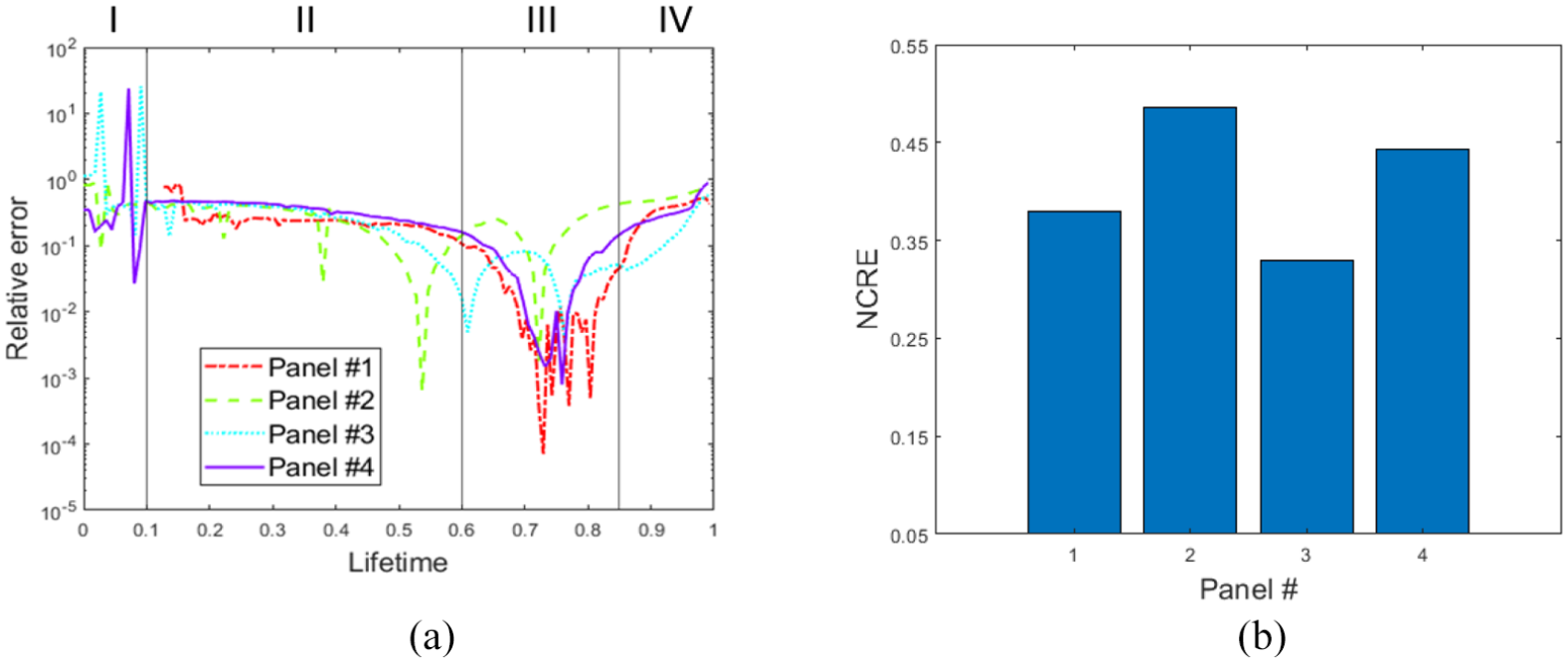
Finally, the relative error $re$ , which is the RUL prediction absolute error normalized by the ground truth RUL, that is, $r e_{k} = | {\bar{r}}_{k} - r_{k} | / r_{k}$ , is computed. Normalizing the prediction error with the ground truth RUL has the effect of increasingly weighting the prediction error as the $EoL$ is approached – one should, however, beware that the final weights approaches infinity, since absolute error is being divided by values nearing zero. In Figure 16(a), the relative error for each panel is illustrated; it can be noticed that all plots share some common features. Indeed, four time-dependent regions can be recognized as follows (a) region I is characterized by high $re$ values featuring the embryonic phase in which the RUL estimates are far from the ground truth value; (b) region II shows the RUL estimates to smoothly approach the ground truth value, which indicates that the evolution model parameters are being correctly filtered; (c) in region III, RUL estimates get abruptly closer to the ground truth values, which is both a consequence of the crack state variables clustering around the true values and the evolution model parameters reaching their target values; and (d) in region IV, the relative accuracy decreases, which might be due to inconsistencies in the evolution model and a because of the normalizing value approaching zero. In Figure 16(b), the normalized cumulative relative error is showing which specimen predicted RUL better fits the ground truth RUL. The cumulative error is calculated from a time value $t_{k} = 0.2 EoL$ onwards, discarding the initial wavy transient. The integral of the relative error is then normalized over the remaining lifetime.

Figure 16.

(a) Relative error of panel specimens RUL estimate and (b) normalized cumulative relative error (NCRE) of panel specimens RUL estimate.

Conclusion

An SIR PF is proposed, being able to simultaneously perform the diagnostic and prognostic tasks relating with FCG in a complex metallic specimen subjected to cyclic loading. Specifically, aluminium alloy stiffened panels, representative of a mid-size helicopter fuselage, are tested. Surrogate models are embedded within the algorithm, enhancing the likelihood assessment as well as the samples projection up to EoL, enabling the algorithm real-time operation. The opportunity for the algorithm online operation is guaranteed by a distributed sensing network measuring the system response. The degradation state estimates involve the crack localization (crack centre coordinates) and assessment, that is, crack size, while the prognostic mission targets the RUL of the specimen, according to a degradation model describing the damage progress in time.

The inherent randomness of FCG is addressed by an augmented state formulation, which allows the tracking of degradation paths which deviates from the algorithm evolution model driving the samples projection ahead in time (i.e. Paris’ law).

The algorithm has been first tested with strain simulated data, which have been polluted with noise to mimic real measurements, showing no difficulties in assessing the crack and comfortably tracking the FCG. Also, the algorithm has demonstrated the ability to update the evolution model parameters, converging to the hidden parameters which were used to generate synthetic FCG patterns. The algorithm has been finally challenged with real data gathered from experimental testing activities involving a set of four identical units, proving to be well suited for the diagnostic and prognostic tasks. In the end, prognostic performance metrics have been employed to provide the user objective tools to evaluate the RUL estimates.

In summary, SMC-based techniques have the potential to satisfy the growing requirements which the modern industry is putting forward. However, despite the promising result which in recent years has been pushing these techniques, there is still much to do. For instance, the authors described how to address the single straight-propagating crack problem; it would be of great interest to develop a framework able to deal with multiple cracks growing simultaneously. It would be equally interesting to analyse crack which do not propagate straightly, as well as crack propagating in solids. Another fundamental issue concerns the selection of the features to be observed in order to maximize the sensitivity to the system degradation. Also, it would be of great interest to analyse the algorithm performance in case of limited sensing, that is, when the sensor network is not fully operational, or one or more sensors stop working. One might also wonder if the algorithm tuning, that is, the hyperparameters setting, can be automated, extending the range of use to non-experienced user; this also avoid the bias which might be induced by the user subjective judgement. These are only a few of the question which arises from the problem, and, as far as the authors know, are not still completely clear.

Footnotes

Declaration of conflicting interests

The author(s) declared no potential conflicts of interest with respect to the research, authorship and/or publication of this article.

Funding

The author(s) received no financial support for the research, authorship and/or publication of this article.

ORCID iD

Demetrio Cristiani

References

Department of USA Defense. Joint service specification guide: aircraft structures (JSSG-2006), 1998, http://everyspec.com/USAF/USAF-General/JSSG-2006_10206/

Bond

Underwood

Adams

, et al. Structural health monitoring–based methodologies for managing uncertainty in aircraft structural life assessment. Struct Heal Monit 2014; 13(6): 621–628.

Jardine

AKS

Lin

Banjevic

A review on machinery diagnostics and prognostics implementing condition-based maintenance. Mech Syst Signal Process 2006; 20(7): 1483–1510.

Kim

Choi

JH.

Practical options for selecting data-driven or physics-based prognostics algorithms with reviews. Reliab Eng Syst Saf 2015; 133: 223–236.

Sikorska

Hodkiewicz

Prognostic modelling options for remaining useful life estimation by industry. Mech Syst Signal Process 2011; 25(5): 1803–1836.

Baraldi

Cadini

Mangili

, et al. Model-based and data-driven prognostics under different available information. Probabilistic Eng Mech 2013; 32: 66–79.

Youn

Wang

, et al. Ensemble of data-driven prognostic algorithms for robust prediction of remaining useful life. Reliab Eng Syst Saf 2012; 103: 120–135.

CC.

Probabilistic models of fatigue crack propagation and their experimental verification. Probabilistic Eng Mech 2004; 19(3): 247–257.

Wang

, et al. Remaining useful life estimation: a review on the statistical data driven approaches. Eur J Oper Res 2011; 213(1): 1–14.

10.

Daigle

Goebel

Model-based prognostics under limited sensing. In: 2010 IEEE aerospace conference proceedings, Big Sky, MT, 6–13 March 2010.

11.

Sankararaman

Ling

Mahadevan

Uncertainty quantification and model validation of fatigue crack growth prediction. Eng Fract Mech 2011; 78(7): 1487–1504.

12.

Gustafsson

Particle filter theory and practice with positioning applications. IEEE Aerosp Electron Syst Mag 2010; 25(7): 53–81.

13.

Doucet

Godsill

Andrieu

On sequential Monte Carlo sampling methods for Bayesian filtering. Stat Comput 2000; 10(3): 197–208.

14.

Arulampalam

Maskell

Gordon

, et al. A tutorial on particle filters for online nonlinear/non-Gaussian Bayesian tracking. IEEE Trans Signal Process 2002; 50(2): 174–188.

15.

Gordon

Salmond

Smith

AFM

. Novel approach to nonlinear/non-Gaussian Bayesian state estimation. IEE Proc F 1993; 140(2): 107–113.

16.

Leser

Hochhalter

Warner

, et al. Sequential Monte Carlo: enabling real-time and high-fidelity prognostics. In: Annual conference of the prognostics and health management society, Philadelphia, PA, 24 September 2018.

17.

Banerjee

Karpenko

Udpa

, et al. Prediction of impact-damage growth in GFRP plates using particle filtering algorithm. Compos Struct 2018; 194: 527–536.

18.

Qian

Yan

Remaining useful life prediction of rolling bearings using an enhanced particle filter. IEEE Trans Instrum Meas 2015; 64(10): 2696–2707.

19.

Cadini

Zio

Avram

Monte Carlo-based filtering for fatigue crack growth estimation. Probabilistic Eng Mech 2009; 24(3): 367–373.

20.

Orchard

Vachtsevanos

GJ.

A particle-filtering approach for on-line fault diagnosis and failure prognosis. Trans Inst Meas Control 2009; 31(3–4): 221–246.

21.

Eftekhar Azam

Bagherinia

Mariani

. Stochastic system identification via particle and sigma-point Kalman filtering. Sci Iran 2012; 19: 982–991.

22.

Tatsis

Tiso

, et al. State estimation of geometrically non-linear systems using reduced-order models. In: Frangopol

Caspeele

Taerwe

(eds) Life-cycle analysis and assessment in civil engineering: towards an integrated vision: proceedings of the 6th international symposium on life-cycle civil engineering (IALCCE 2018). Boca Raton, FL: CRC Press, 2018, pp. 219–227.

23.

Sen

Bhattacharya

Progressive damage identification using dual extended Kalman filter. Acta Mech 2016; 227: 2099–2109.

24.

Mylonas

Abdallah

Chatzi

Surrogate modelling for fatigue damage of wind-turbine blades using polynomial chaos expansions and non-negative matrix factorization. IABSE Symp Rep 2017; 109: 801–808.

25.

Paris

Erdogan

A critical analysis of crack propagation laws. J Fluids Eng Trans ASME 1963; 85(4): 528–533.

26.

Virkler

Hillberry

Goel

PK.

The statistical nature of fatigue crack propagation. J Eng Mater Technol Trans ASME 1979; 101(2): 148–153.

27.

Wang

GS.

Intrinsic statistical characteristics of fatigue crack growth rate. Eng Fract Mech 1995; 51(5): 787–803.

28.

Dubourg

Sudret

Deheeger

Metamodel-based importance sampling for structural reliability analysis. Probabilistic Eng Mech 2013; 33: 47–57.

29.

Vega

Madarshahian

Todd

. A neural network surrogate model for structural health monitoring of miter gates in navigation locks. In: Barthorpe

(ed.) Conference proceedings of the society for experimental mechanics series. Cham: Springer, 2020, pp. 93–98.

30.

Leser

Hochhalter, Warner

, et al. Probabilistic fatigue damage prognosis using surrogate models trained via three-dimensional finite element analysis. Struct Heal Monit 2017; 16(3): 291–308.

31.

Warner

Hochhalter

Leser

, et al. A computationally-efficient inverse approach to probabilistic strain-based damage diagnosis. In: Proceedings of the annual conference of the prognostics and health management society (PHM 2016), Denver, CO, 3–6 October 2016, pp. 55–69. Prognostics and Health Management Society.

32.

Keprate

Ratnayake

RMC

Sankararaman

Comparison of various surrogate models to predict stress intensity factor of a crack propagating in offshore piping. J Offshore Mech Arct Eng 2017; 139(6): 061401.

33.

Hombal

Ling

Wolfe

, et al. Surrogate modeling of crack growth. In: Safety, reliability, risk and life-cycle performance of structures and infrastructures proceedings of the 11th international conference on structural safety and reliability, ICOSSAR 2013, New York, NY, 16–20 June 2013, pp. 3237–3244. Taylor & Francis Group, https://www.taylorfrancis.com/books/9780429227950

34.

Ocampo

Millwater

. Probabilistic damage tolerance for small airplanes using a linear-elastic crack growth fracture mechanics surrogate model. In: 54th AIAA/ASME/ASCE/AHS/ASC structures, structural dynamics, and materials conference, Boston, MA, 8–11 April 2013.

35.

Pais

Viana

FAC

Kim

NH.

Enabling high-order integration of fatigue crack growth with surrogate modeling. Int J Fatigue 2012; 43: 150–159.

36.

Gao

Guo

XF.

Crack identification based on Kriging surrogate model. Struct Eng Mech 2012; 41(1): 25–41.

37.

Liu

West

Combined parameter and state estimation in simulation-based filtering. In: Doucet

de Freitas

Gordon

(eds) Sequential Monte Carlo methods in practice. New York: Springer, 2001, pp. 197–223.

38.

Sbarufatti

Manes

Giglio

Application of sensor technologies for local and distributed structural health monitoring. Struct Control Heal Monit 2014; 21(7): 1057–1083.

39.

Hol

Schon

Gustafsson

. On resampling algorithms for particle filters. In: 2006 IEEE nonlinear statistical signal processing workshop, Cambridge, 13–15 September 2006, pp. 79–82. New York: IEEE.

40.

Walker

. The effect of stress ratio during crack propagation and fatigue for 2024-T3 and 7075-T6 aluminum. In: Rosenfeld

(ed.) Effects of environment and complex load history on fatigue life. West Conshohocken, PA: ASTM International, 1970, pp. 1–14.

41.

Beden

Abdullah

Ariffin

AK.

Review of fatigue crack propagation models for metallic components. Eur J Sci Res 2009; 28(3): 364–397.

42.

Corbetta

Sbarufatti

Giglio

, et al. Optimization of nonlinear, non-Gaussian Bayesian filtering for diagnosis and prognosis of monotonic degradation processes. Mech Syst Signal Process 2018; 104: 305–322.

43.

Annis

Probabilistic life prediction isn’t as easy as it looks. J ASTM Int 2004; 1(2): 1–12.

44.

Poe

Jr.

Stress- intensity factor for a cracked sheet with riveted and uniformly spaced stringers. NASA Technical Report R-358, 1971.

45.

Saxena

Celaya

Saha

, et al. On applying the prognostic performance metrics. In: Annual conference of the prognostics and health management society (PHM 2009), 2009.

46.

Saxena

Celaya

Saha

, et al. Metrics for offline evaluation of prognostic performance. Int J Progn Heal Manag 2010; 1(1): 1–20.