A review on diagnostic and prognostic approaches for gears

Abstract

Prognostics and health management has become a significant part of component life-cycle in modern industries. The prognostics and health management framework is implemented in the industries to identify the fault type, assess fault severity, and predict the future state or remaining useful life to optimize the maintenance activities. Three significant aspects of a prognostics and health management framework are diagnostics, prognostics, and decision making. This article presents a review of different types of diagnostic and prognostic approaches (i.e. physics-based, data-driven, and hybrid approaches) developed for the gears. The flow of information between diagnostics and prognostics parts of the framework is briefly discussed. Regarding the physics-based approaches, this article discusses different physics-based diagnostic and prognostic models developed for different types of gear failure modes such as crack, pitting, and wear. In the data-driven approaches, the article attempts to summarize the data processing techniques used for extracting fault-related information from the recorded raw vibration signal, health indicators developed for different kinds of gear failure modes, processing/selection approaches for best health indicators, fault classification, and fault prognostic models particularly developed for the gear. The article discusses how a hybrid approach can be developed by the integration of a data-driven diagnostics approach and a physics-based prognostics approach. Finally, uncertainty quantification of prognostic approaches, performance evaluation metrics, decision-making strategies, and future research and development perspectives are discussed. This article focuses on the diagnostic and prognostic approaches developed for gears, given the fact that these approaches for other components such as bearing and batteries are reviewed in the past.

Keywords

Gear vibration diagnostics prognostics condition monitoring

Introduction

The power transmission (e.g. speed and torque conversion) from one shaft to another shaft can be achieved using a gearbox, chain-sprocket mechanism, belt-pulley mechanism, and so on. Compared to the gearbox, the belt-pulley and chain-sprocket arrangements are cost-effective and easy to use. However, these mechanisms have many disadvantages such as less service life, low load capacity, and less velocity ratio, and mostly preferred when power needs to be transmitted between shafts with large center distance. Comparatively, the gearbox is most widely used for power transmission due to large and constant velocity ratio, compact construction, higher transmission efficiency, large power transmission, longer service life, and so on. Considering its wider use in the industry, the uninterrupted and quiet operation of the gearbox is of paramount importance.

In a survey,¹ it is found that 74.7% of time gears fail due to service-related causes (user) and 25.3% of the time they fail due to design errors, incorrect manufacturing processes leading to material defects, heat treatment errors, manufacturing defects, and so on. The reasons for service-related failure are continuous overloading, higher levels of speed and torque fluctuations, improper assembly/alignment, impact loading, improper lubrication, ingress of foreign material in the tooth contact area, incorrect handling, operator error, and so on. The failure statistics in several key application areas are a pointer to a need for a systematic and concerted effort on the diagnostics and prognostics approaches. In helicopter transmission system failure, 19.1% of the failures are found due to gears.² In some applications, even if the gear failures are relatively less frequent, the downtime and associated costs are relatively higher. For example, in a survey on wind power systems, it was found that although the gears have only 9.8% of the total failure, they add up to 19.4% of the complete downtime of a wind turbine.³ In addition, the unexpected or unplanned shutdown of the gearbox may lead to loss of human life in some applications. For example, in April 2009, 16 people lost lives due to the catastrophic failure of the gearbox of the North Sea helicopter.⁴ In summary, the failure/degradation of a geared system increases unplanned outages, reduces productivity, increases operating and maintenance costs, and so on. Hence, it is critical to have a good condition monitoring (CM) system in order to reduce gear failure. Prognostics and health management (PHM) is an emerging discipline for gear condition assessment. The implementation of the PHM framework allows a cost-effective maintenance practice as it can give indications and warning prior to collateral damages and help in improvement in availability and reliability.⁵

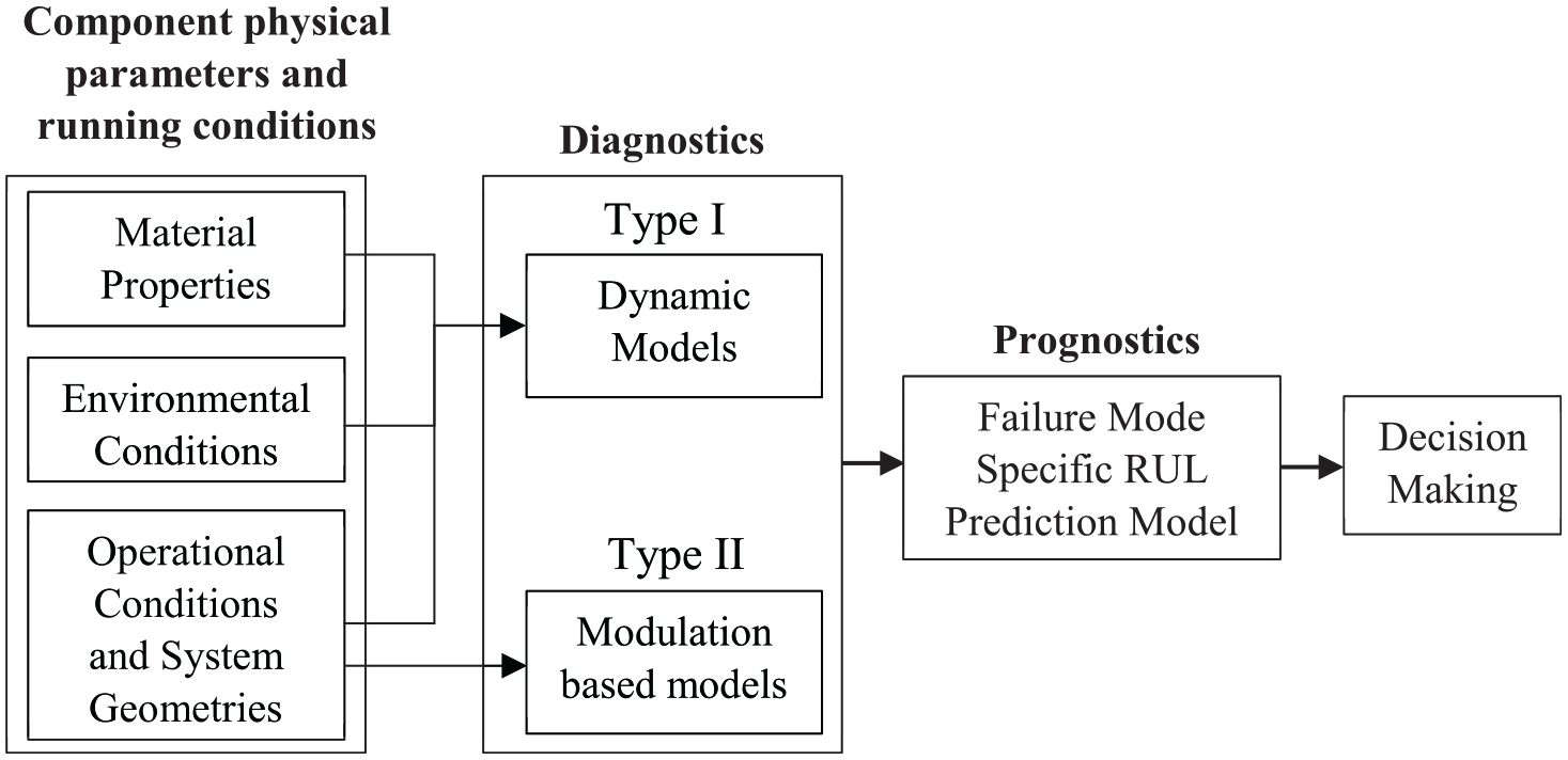
Diagnostics, prognostics, and decision making/health management are three main parts of a PHM framework. The diagnostic process deals with fault detection, identification, classification, and so on and provides the current health stage (e.g. zero pitting, initial pitting, medium pitting, severe pitting on the gear tooth surface) information of the gear. Prognostics is the remaining useful life (RUL) prediction of a gear based on their current and historical health condition. More specifically, based on the current loading condition and expected future operational and environmental conditions, prognostic approaches predict the RUL by estimating the development of a fault on the gear tooth surface given the present level of degradation.⁶ The prognostic approaches in a PHM framework can be implemented in three different ways using physics-based approaches, sensor data-driven approaches, and hybrid approaches (a combination of sensor data-driven and physics-based approaches). The decision making/health management process involves the actions implemented based on the estimate of the current health state and the predicted RUL. The decision-making step ensures a reduction in life-cycle costs, safe operation or reducing the catastrophic failures, increases system availability by expanding the maintenance cycles, reduction in inspections, timely repair actions, and improves design and logistical support.⁶ The same decision-making procedure can be implemented for any type of PHM framework, that is, physics-based, data-driven, or hybrid.

Some researchers^7,8 believe that diagnostics and prognostics need to be considered as an integrated process, whereas others^9–13 are of the view that diagnostics and prognostics can be achieved separately. However, it is indeed true that the performance of prognostic approaches depends on the type and accuracy of the diagnostics output (i.e. type of health indicators (HIs), fault types/severity, and its progression rate), especially for components that have multiple failure behaviors/modes. In fact, diagnostic can be independent of prognostic, not the vice versa. Different failure modes have different dynamics of initiation and rate of propagation. Hence, prognostics approach developed for one kind of failure mode may not work for different kinds of failure modes. If a component has a single failure mode, then prognostics might be performed independently without the need for diagnostics output. Hence, for the prognostics, regardless of the type of approach (physics-based, data-driven, or hybrid), diagnostics is the first and critical step.

Some researchers have already reviewed some aspects of the PHM framework for gear. For example, Liang et al.¹⁴ have reviewed dynamic modeling of the gear faults while a review on the physics-based prognostic approaches for many of the gear failure modes is presented by Cubillo et al.¹⁵ The data-driven prognostic approaches implemented for rotating machinery are summarized in previous studies,^{11,12,16–19} wherein the review work is more aligned with the bearings instead of gears. Many of the time domain-based HIs developed for gear fault diagnostics are summarized in previous studies.^20–25 The existing review articles on gear diagnostics and prognostics have a specific and limited scope and many aspects are not elaborately discussed. In light of the existing research articles mentioned above, the following significant contributions are made in this article:

This article presents a comprehensive review of diagnostic and prognostic approaches developed for different types of PHM framework for gears: from physics-based, data-driven, to hybrid approaches.

In the physics-based PHM framework (section “Physics-based approaches”), a description of different gear failure modes, an overview of modulation-based and dynamic models used for gear fault diagnostics is given. In addition, the prognostic approaches developed for most reported gear failure modes such as crack, pitting, and wear are reviewed. The model parameter updating algorithms developed for improvement in accuracy of the physics-based prognostic approaches are also discussed.

Although this review paper is more aligned in the direction of approaches developed based on vibration signal, the pros and cons of different types of sensors used for gear CM are discussed in the data-driven PHM framework section (section “Data-driven approaches”). In addition, in this section, a variety of data processing methods for gear raw vibration signal, time domain, frequency domain, and time-frequency domain-based HIs developed based on the processed/raw vibration signal, techniques used for processing/selection of best HIs, machine learning and deep learning approaches developed for gear fault severity/type classification, and fault prognostics are briefly reviewed.

The hybrid prognostic approaches developed for different kinds of gear failure modes are reviewed (section “Hybrid approaches”). It has been noticed that not many hybrid prognostic approaches are developed for gears. The present review attempts to cover all the major reported hybrid approaches developed so far.

An overview of uncertainty quantification of prognostic approaches (section “Uncertainty quantification of prognostic approaches”), performance evaluation metrics (section “Performance evaluation metrics”) used for classification and prognostic approaches, and post prognostics decision process (section “Post prognostics decision making/health management process”) is also given. Future research possibilities and challenges in the direction of gear diagnostics and prognostics are discussed (section “Concluding remarks”).

Majority of the diagnostic and prognostic approaches for gears are developed based on the vibration signal. In general, it is observed that the vibration signal contains most of the information related to the gear dynamics and the changes in the dynamic response due to gear tooth degradation. Hence, this work focuses on the review of the vibration signal–based diagnostic and prognostic approaches developed so far.

Physics-based approaches

In the physics-based approaches, component health is assessed by solving a set of equations based on the physical laws and the knowledge of engineering and science.¹¹ The physics-based approaches are very important if accuracy is a critical factor and testing is restricted.¹⁵ The physics-based approaches are failure mode-specific. A gear may fail in various modes and these failure modes in the order of decreasing frequency can be divided into four groups: fatigue, impact, wear, and stress rupture.^1,26

Fatigue: The repeating cyclic stresses lower than ultimate tensile strength cause cracking of the surface, which results in fatigue failure. The fatigue failure can be divided mainly into two categories: tooth bending fatigue and surface contact fatigue.

Tooth bending fatigue: It results from a crack originating in the root section of the gear tooth. Non-metallic inclusions near the surface, imperfections in the root section of gear tooth, and so on. are reasons for the bending fatigue. The subsequent progression of crack originated at the root section causes fracture of the gear tooth surface.

Surface contact fatigue: When two surfaces roll or roll and slide against one another with sufficient contact force, the maximum shear stress is developed slightly below the contacting surface. The surface contact fatigue is initiated by this maximum shear stress and causes the cracking of the surface. These cracks propagate at a shallow angle and form a pit when the contact stresses exceed the surface fatigue strength of the material.²⁷

Impact: Due to sudden shock load, the tooth gets fractured within a few cycles and results in impact failure. This kind of failure is random and hence not many physics-based diagnostic and prognostic studies are reported for this category of gear failures.

Wear: Metal-to-metal contact due to lack of oil film, ingress of abrasive particles in oil, and so on cause removal of material more or less uniformly from the active gear tooth surface and results in wear failure.

Stress rupture: The internal residual stresses build to a magnitude beyond the strength of the material cause rupture of the gear tooth.

The failure modes discussed above have several subcategories.^1,26 Among the gear failure modes, a majority of gear failures appear as tooth crack/fracture, pitting, and wear failure mode. Hence, most of the diagnostic and prognostic approaches are developed for these failure modes. In this article, physics-based diagnostic and prognostic methodologies developed for these failure modes are reviewed.

Physics-based diagnostic approaches

The diagnostics cannot be pure physics-based as the physical sensor data is always required to assess the gear condition. For example, a cracked or broken tooth might excite a gear-pair natural frequency every time it meshes, increasing the harmonics of shaft speed in the vicinity of the resonance.²⁸ The gear pair natural frequency can be estimated theoretically using physics-based model. However, to know whether the frequency is indeed excited and appears in the actual vibration signal in the geared system, the vibration sensor data is required. Most of the physics-based diagnostic approaches build a virtual dynamic system that models and mimics the complete gearbox system based on the physical understanding of that system. For diagnostics, the output of the physics-based model is compared with the sensor data output and a fault is detected. The physics-based diagnostic models can be divided into two categories: modulation-based models and dynamic models.¹⁴ In the modulation-based models,^29,30 amplitude, frequency, and phase modulation characteristics of the gear vibration signal are analyzed. The dynamic models are based on the lumped parameter model of the elements of the gearbox, the gear mesh, and associated elements. The development of both modulation-based and dynamic models is discussed hereunder.

Modulation-based models

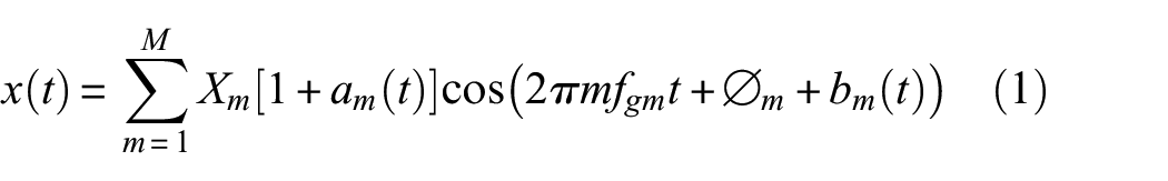
The vibration signal obtained from a healthy geared rotor system comprises shaft rotational frequency, gear mesh frequency (GMF), and their harmonics due to deviations from the ideal tooth profile, residual rotor unbalance, transmission error, and so on.^29,31,32 The amplitude modulation (AM) and frequency modulation (FM) of gear carrier signal generate the sidebands around GMF and its harmonics in a healthy geared rotor system. Figure 1 shows a typical healthy geared pair vibration signal obtained from a gearbox test rig.³² The frequency spectra in Figure 1(c) and (d) show the sidebands, GMF and its harmonics, and sidebands around the GMF. In the healthy stage, the gear carrier signal is modulated due to reasons such as fluctuation in load/speed, riding of the gear on an eccentric gear or on a misaligned shaft and so on.³³ Hence, the vibration signal $x (t)$ for a gear can be expressed as^30,34

x (t) = \sum_{m = 1}^{M} X_{m} [1 + a_{m} (t)] \cos (2 π m f_{gm} t + Ø_{m} + b_{m} (t))

(1)

where, $f_{gm} = N f_{s}$ is the GMF, m = 1, 2, 3, …, M represents the number of the harmonic, $f_{s}$ is the rotating speed, $N$ is the number of teeth, $Ø_{m}$ is the initial phase angle of the $m th$ meshing harmonic, $X_{m}$ is the amplitude of the $m th$ harmonic, and $a_{m} (t)$ and $b_{m} (t)$ are the AM and FM functions, respectively.

Figure 1.

A typical gear vibration signal in (a) time domain, (b) time domain zoomed view, (c) frequency domain, and (d) frequency domain zoomed around the fundamental GMF.

The gear vibration of varying AM, FM, and phase angle can be simulated/generated using equation (1). In general, the signal simulated using a modulation-based model helps in the understanding of the gear vibration signal obtained in a healthy stage and particular fault severity stage. These models highlight the key characteristics of the gear vibration signal expected in the experimental measurements or field data. The gear mesh stiffness changes due to the presence of a defect on the gear tooth surface. Depending on the type of defect, these changes can be seen as changes in the amplitude of the GMF and its harmonics or change in the AM and FM, and phase effect on the gear mesh vibrations.

For example, the presence of wear on either side of the pitch point tends to affect the tooth meshing frequency and its harmonics. The type of profile error generated because of the surface wear distorts the gear meshing stiffness cycle. The effect of tooth wear is more noticeable at the higher harmonics of GMF compared to the fundamental GMF itself. Thus, at least the first three harmonics of the GMF should be considered for wear detection in early stages.²⁹ Similarly, defects such as pitting cause a non-uniformity in tooth spacing leading to the changes in the gear angular velocity as a function of the rotation. This effect may causes the FM of the gear mesh carrier signal. In addition, non-uniform tooth spacing also increases the fluctuation in torque and hence increases the AM. The sidebands are thus produced as a combined effect of AM and/or FM, both resulting from the same fault.²⁹ The increase in the amplitude of the sidebands and their families are often used for gear pitting detection.³² Due to phase relations on either side of the carrier frequency, sidebands may combine to give reinforcement on one side and cancelation on the other, depending on the initial phase relationships of the AM and FM. Because of this reason, the sidebands structure in gear spectra is often unsymmetrical.²⁹ In addition, the presence of pitting reduces the GMF amplitude due to increase in the FM of the gear carrier signal. However, GMF amplitude is not affected due to increase in the AM.³² McFadden³⁰ showed the importance of modulation for early detection of the defect such as fatigue crack. A very high-phase lag in the signal due to variation in the mesh point is observed when the affected part of the gear comes under load. In summary, the studies reported by McFadden,³⁰ Randall,²⁹ and Kundu et al.³² can be referred for a better understanding of the modulation-based models developed for analyzing the gear vibration generated because of failure modes such as crack, wear, and pitting, respectively.

Dynamic models

The dynamic models use physical law such as equilibrium, conservation of energy, and Newton’s laws of motion to simulate gearbox vibration response in different health conditions.¹⁴ In the dynamic models, various health conditions of the gear can be mathematically simulated. The dynamic models for the geared system are developed using many different ways. Lumped parameter modeling (LPM) and finite element modeling (FEM) are the most popular among them. In LPM, components (e.g. shaft, bearing, gear) in a geared system are considered to be solid and modeled as a combination of lumped mass, stiffness, and damping parameters. In FEM, a similar analogy is used in which mass, stiffness, and damping parameters are distributed on mesh elements and assemble them to form a complete mass, stiffness, and damping matrices for each component. Both kinds of modeling give similar results if boundary conditions and degree of discretization are properly defined.¹⁴ However, the FEM is much computationally expensive compared to the LPM.

The time-varying mesh stiffness is one of the main sources of vibration in a gear transmission system. Based on the change in the gear mesh stiffness and its variation for a faulty gear, the gearbox vibration response changes. The dynamic model involves the time-dependent gear mesh stiffness, which can be modeled following a square waveform method, potential energy method, finite element method, experimental method, and so on.¹⁴

Square waveform method for gear mesh stiffness evaluation: This approach is the easiest to model the gear mesh stiffness. The gear mesh stiffness is approximated using a square waveform periodic function. The time duration for one revolution divided by the number of teeth represents the period of the square waveform.

Potential energy method for gear mesh stiffness evaluation: The gear mesh stiffness is approximated by assuming the gear tooth as a cantilever beam. The gear mesh stiffness is estimated based on the solid mechanics of the beam. In this method, the contribution of bending, shear, axial compressive, and Hertzian contact is usually analyzed for stiffness evaluation.

Finite element method for gear mesh stiffness evaluation: This approach numerically estimates the gear mesh stiffness by discretization of the gear pair. The finite element method is a time-consuming and computationally expensive method. The accuracy of these methods depends on the degree of discretization, mesh density, and choice of element type.

The experimental method for gear mesh stiffness evaluation: Methods such as photo elasticity,³⁵ dynamic speckle photography,³⁶ and strain gauge³⁷ are used for experimental estimation of gear mesh stiffness.

The dynamic models help in simulating the response of the geared system being monitored. The indicator extracted based on the dynamic response can be used for gear fault diagnostics. If properly modeled, the model can simulate the component failure condition under any given speed and load profile.¹⁸ Hence, the dynamic model reduces the time and expenses associated with seeding the physical damage/fault on the actual component (gear). However, the dynamic model has two major drawbacks. First, some factors such as misalignment, gear surface quality, oil quality, and clearance are difficult to model. Hence, the experimental and the simulated vibration response from the dynamic model seldom match exactly. Second, the dynamic models are expensive in terms of modeling efforts and computational time, particularly for complex gearing systems.¹⁶Åkerblom³⁸ and Liang et al.¹⁴ have given a detailed description of dynamic models for geared systems and hence is not covered in detail in the present review.

Physics-based prognostic approaches

Based on the mathematical modeling of the degradation process for a particular failure mode, the physics-based prognostic approaches predict when the damage in gear crosses a predefined threshold of failure. The description of prognostic approaches used for different kinds of gear failure mode is given in the subsequent sections.

Crack

The fatigue crack in a gear tooth is mainly caused by high cycle fatigue. The Paris power law equation describes the crack growth that can be used for estimating the RUL. The Paris power law equation for modeling the crack growth is given by³⁹

\frac{da}{dN} = C Δ K^{m}

(2)

where $a$ is the crack size, $N$ is the number of cycles, $C and m$ are the model parameters that are estimated based on the available crack growth data, and $Δ K$ is the stress intensity factor (SIF). The SIF is given by

Δ K = Y Δ σ {(π a)}^{0.5}

(3)

where $Y$ is the correction factor that depends on the geometry, flaw size, and shape and $Δ σ$ is the stress range. The SIF determines the stress distribution near the crack tip and accurate calculation of SIF is very important for accurate assessment of crack propagation or RUL prediction. Different techniques are used by different researchers^40–45 for SIF estimation. For calculation of the RUL of the gear tooth based on initial crack length $(a_{o})$ and threshold crack length $(a_{th})$ , equation (2) can be written for number of cycles of failure as⁴⁶

N = \frac{2}{(m - 2) C Y^{m} {(Δ σ)}^{m} {(π)}^{\frac{m}{2}}} ({a_{o}}^{1 - \frac{m}{2}} - {a_{th}}^{1 - \frac{m}{2}})

(4)

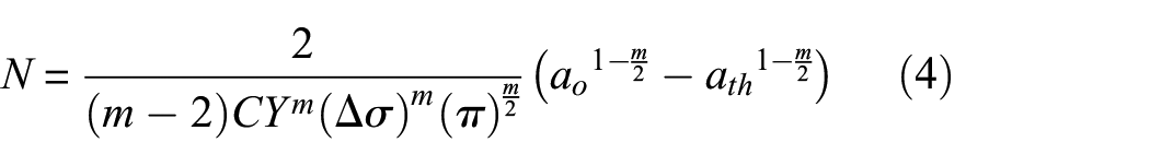
The Paris power law equation is the most widely used for estimation of crack propagation in gear tooth. For example, in the literature,^45,47 the tooth crack growth was estimated using this equation. For a particular crack length, gear mesh stiffness was estimated using the potential energy method and the stiffness is input to the gear dynamic model for estimating the stress variation. Based on this variation, the SIF was estimated using equation (3) and then the fracture mechanics-based model (equation (4)) was used for the RUL prediction. Li and colleagues^45,47 give an overview of a combined physics-based diagnostic and prognostic approach developed for gear subjected to crack failure mode. Endeshaw et al.⁴⁸ proposed an approach for crack propagation in gears considering uncertainties in loading and material properties. The uncertainties in loading and material properties are incorporated in the gear dynamic model. Based on the gear dynamic model, it was found that an increase in crack length reduces gear mesh stiffness and, as a result, increases the dynamic force on the gear tooth. The calculated dynamic force is input to the finite element model for calculation of the SIF and gear crack propagation life was predicted using the Paris power law equation. Many researchers used the FEM-based software for estimation of the SIF used in the Paris power law equation instead of developing a dynamic model. For example, Glodež et al.⁴⁹ used the FEM program in FRANC2D software for simulating the fatigue crack growth in the gear tooth root. The virtual crack extension method was used for simulating the crack propagation path. Chen et al.⁵⁰ analyzed the propagation path and failure behavior of cracked gears under different initial angles. A decrease in gear mesh stiffness was observed with an increase in the initial crack angle. The crack propagation path through the gear rim was found more serious as compared to the crack propagation path through the teeth. In addition, in this study, a relationship between the gear crack propagation process and degradation level is established. For a particular initial crack angle, crack propagation path and the crack length were predicted using FEM. Based on the predicted path and length, the gear vibration response was simulated using a gear dynamic model. The degradation parameters such as root mean square (RMS) and kurtosis were extracted using the simulated vibration response. Subsequently, the relation between the extracted parameters and crack propagation path and length was established.

In most of the studies, crack is virtually initiated at a point and in the direction of maximum principal stress in the gear tooth root. Estimation of the number of cycles required for the fatigue crack initiation is important during the calculation of the total gear life. The strain life method based on FEM was used by Glodež et al.⁴⁹ to estimate the number of stress cycles required for the fatigue crack initiation. However, Lin et al.⁵¹ used the power density method for estimation of the fatigue crack initiation life.

These works are further extended for a more comprehensive analysis of gear fatigue crack propagation. For example, Lewicki et al.⁵² considered the effect of moving gear tooth load for the prediction of crack propagation. Podrug et al.⁴³ considered the effect of gear rim thickness, crack closure, and change in forces during rotation while the prediction of gear tooth cracks propagation life. Agarwal et al.⁵³ studied the phenomena of fatigue crack propagation in the presence of inclusion in the gear tooth root. For the hard inclusions near to the original crack paths, the crack propagation was observed to be slower. The finite element model using the Paris power law equation, gear crack path, and fatigue life was predicted. In order to reduce the computational requirement of the FEM-based gear crack life prediction methodology, Gueye et al.⁵⁴ proposed a pseudo evolutionary structural optimization approach. Čular et al.⁵⁵ proposed a strain-life approach that differs from the above studies for gear bending (crack) fatigue life prediction.

The Paris power law equation only holds when the crack growth rate is significant and not valid when the crack growth is not significant or become unstable. Alternate models such as Foreman law,^56–58 which are the extended version of the Paris power law equation, can also be used for gear crack growth prediction. Studies on the development of various fatigue crack growth models are detailed in Pugno et al.⁵⁹

Pitting

The subsurface crack propagation under cyclic loading allows the material to break from its surface and results in pit formation.^60–64 Hence, the Paris power law equation (equation (2)) used for modeling the crack growth can also be utilized to estimate the propagation of the surface-breaking crack, which results in a pit formation. Blake and Cheng⁶⁴ used such a model for predicting the initiation of pitting. As discussed earlier, the surface fatigue failure/pitting is initiated by the maximum shear stress acting below the gear tooth surface.⁶⁵ Hence, instead of using the normal stress (mode I crack propagation), the shear stress is used in equation (2) for predicting the subsurface breaking crack propagation, which is also termed as mode II crack propagation. This study was further extended by Blake and Cheng,⁶⁶ in which a predictive pit growth model was proposed for estimating the failure probabilities and service life for gears. Aslantaş and Taşgetiren⁶⁷ considered both mode I and mode II crack propagation SIF for predicting the initiation of pitting. Based on the finite element model developed in FRANC2D simulation software, the linear elastic fracture mechanics approach is used for gear life prediction with pitting failure mode. Glodež et al.⁶⁸ proposed a new model in which a finite element-based virtual crack extension method was used for predicting the initiation of pitting on gear tooth surface. The conventional pitting life prediction model is developed based on assumptions that gear tooth surface are ideally smooth without lubrication. Fajdiga et al.⁶² proposed a numerical computational model in which the influence of lubricant pressure acting on the subsurface crack faces, which ultimately results in pitting, is studied. The effect of lubricant pressure within the crack is very important because it refers to mode I crack opening. In addition, in this study, the effect of Hertzian contact pressure, friction between contact surfaces, elastohydrodynamic lubrication (EHL) condition, the fluid trapped in the crack, and residual stresses due to heat treatment of the material on the gear pitting life is investigated. Zhu et al.⁶⁹ proposed the pitting life prediction model based on a three-dimensional (3D) line contact mixed EHL analysis and subsurface Von Mises stress calculation. The fatigue life prediction proposed by Zaretsky⁷⁰ was used for gear pitting life estimation. Li and Kahraman⁷¹ extended these studies and developed a complex physics-based model for predicting the gear pitting initiation. In this study, the effect of tooth force, rotational speed, lubricant properties, lubricant temperature, surface roughness, residual stress, and material fatigue strength on gear pitting initiation is evaluated. In addition, in this study, a micro-pitting severity index is proposed for defining the pitting severity level. Li et al.⁷² also developed a similar model for gear pitting initiation prediction.

Correlation between gear dynamics and gear tribology is very important for the gear life prediction. The close correlation between gear tribology and gear dynamics is also called as gear tribo-dynamics. Li and Anisetti⁷³ proposed a turbo-dynamic contact fatigue model for gear pitting initiation prediction. The governing equations of motion developed based on gear dynamic model and mixed EHL model are coupled together. Based on the coupled equations, normal pressure and tangential shear stresses are estimated below the surface and incorporated into the fracture mechanics model for life estimation. Multiaxial fatigue criterion was used for predicting the contact fatigue crack initiation life (pitting initiation). Depending on the gear contact ratio, the load is shared between multiple gear teeth. Moallem et al.²⁷ introduced this load-sharing concept in gear pitting life estimation. Yin et al.⁶¹ developed a 3D dynamic finite element analysis model for gear pitting life prediction in ANSYS workbench. In this work, the plastic deformation of each element near the subsurface crack is used for subsurface crack propagation. This accumulated plastic strain is replaced with SIF in the Paris power law equation for pitting initiation prediction for gear under heavily loaded lubricated contacts.

Although models for predicting the initiation of pitting are proposed, a model for predicting the growth of existing pit on the gear tooth surface is not yet available. The model developed for representing the bearing spall growth can also be adapted/extended to represent the pit growth rate on the gear tooth surface, both being surface fatigue phenomena. The spall growth in the rolling element bearing can be represented with a small modification in the Paris power law crack growth equation as^74,75

\frac{dD}{dN} = C D^{m}

(5)

The above equation indicates that the rate of growth of the defect is related to the instantaneous defect area D under constant operating condition.⁷⁴

Wear

Apart from a fatigue surface crack, tooth contact surface wear (occurs due to sliding contact) may be modeled. A very thin lubrication film separates the contact surfaces of the gear teeth while in the mesh. However, this film is insufficient to avoid the direct asperity contact between two gear mating surfaces that results in the wear on the mating surfaces. Due to continuous wear, the gear tooth becomes thinner and increases the vibration level. Zhu et al.⁷⁶ presented a summary of the empirical and theoretical wear laws developed for wear rate progression estimation. The wear progression on the gear tooth surface is usually modeled by Archard’s law.⁷⁷ According to this law, the accumulated wear at a particular point on the gear tooth surface under rubbing dry, mixed, or boundary lubricated surface can be expressed by integrating the following equation⁷⁸

\frac{dh}{ds} = f (p, v, T, materials, lubrication, \dots)

(6)

where $h$ is the wear depth, $s$ is the sliding distance, $p$ is the local contact pressure on mating surfaces, $v$ is the sliding speed, and $T$ is the local surface temperature. For a local point on one of the gear tooth mating surfaces, equation (6) can be expressed as⁷⁸

\frac{dh}{ds} = kp

(7)

where $k$ is the dimensionless wear coefficient that determines the wear rate. The wear coefficient parameter depends on the type of material and is usually estimated based on wear rate progression experiments for the particular material and lubrication conditions. In equation (6), the sliding distance can be calculated by gear geometry calculations based on the involute profile.⁷⁹ Different methods are used to estimate the local contact pressure on the gear tooth mating surfaces. For example, Shifeng and Cheng⁸⁰ and Zhao et al.⁷⁹ used the Hertz theory and Flodin and Andersson⁷⁸ used the Winkler surface model for contact pressure estimation.

The wear on the gear tooth surface is highly affected by the lubrication condition and in most of the case studies on gear wear, partial-EHL condition is considered. For exact determination of wear rate progression on the gear tooth surface, equation (6) can be modified. For example, Wu and Cheng⁸¹ considered the thermal desorption and oxidative wear mechanism at low and elevated asperity contact temperature, respectively, during the determination of wear rate progression in a spur gear under partial-EHL lubrication condition. This study was further extended by Shifeng and Cheng⁸⁰ in which a gear tooth profile was analyzed by consideration of gear dynamics. The equivalent wear rate and tooth wear profile along the line of action were analyzed in this study. In both addendum and dedendum portion of the gear tooth surfaces, the material was removed. However, the highest wear was found at the beginning of gear engagements. Bajpai et al.⁸² combined the finite element-based gear contact mechanics model and Archard’s wear model for predicting the wear evolution on the spur and helical gear tooth surfaces. This study is focused on developing the wear prediction model considering the manufacturing and assembly imperfections and intentional surface modifications. Liu et al.⁸³ developed a comprehensive contact fatigue wear model in which the effect of loading condition, lubrication condition (mixed-EHL modeling), initial surface roughness, residual stress, and hardness on gear wear life is investigated.

In the above studies, the wear coefficient parameter $k$ was assumed to be constant for a particular material. However, the surface and lubrication conditions change with the evolution of the wear and hence the fixed value of the wear coefficient does not consider the uncertainty in the wear evolution process. Zhao et al.⁷⁹ overcome this problem by considering the wear coefficient as a random variable. In this study, for the exact estimation of the wear evolution process, the wear coefficient was changed according to wear progression data obtained specific to the component of interest and operating condition. Hong et al.⁸⁴ presented a nonlinear dynamic model of the wear process for life estimation of gear subjected to surface wear.

After a number of cycles, fatigue wear leads to the development of subsurface crack on the gear tooth surface. This subsurface crack propagation develops into pitting.^15,83 Ghosh et al.⁸⁵ developed a correlation between wear and subsurface crack propagation

\log (N) = alog (Q) + b

(8)

where N is the number of cycles to failure in pitting, Q is the contact shear stress, which depends on the coefficient of friction and wear rate, and a and b are constants obtained based on experimental data.

In summary, Table 1 lists the issues addressed by various researchers on the development of physics-based prognostic approaches for different kinds of failure modes in gear.

Table 1.

Physics-based approaches implemented by various researchers for gear damage growth rate estimation.

Failure mode	Reference	Specific issue addressed
Crack	45,47	Integrate physics-based diagnostic (potential energy-based dynamic model) and prognostic approach (Paris power law)
	48	Uncertainties in loading and material properties
	49	Proposed virtual crack extension method; strain-life approach for estimation of fatigue crack initiation life
	50	Effect of initial crack angle on gear life and crack propagation path
	51	Approach for fatigue crack initiation life prediction using power density method
	52	Effect of moving gear tooth load on gear life
	43	Effect of gear rim thickness, crack closure effect, and change in forces during rotation on gear life
	53	Effect of inclusions on gear crack propagation path and life
	54	A pseudo evolutionary structural optimization approach for reducing the computation time in FEM-based gear tooth crack modeling
	55	Strain-life approach for gear life prediction
Pitting	64,66	Mode II subsurface crack propagation study for pitting initiation and failure probability estimation model
	67	FEM-based study considering mode I and mode II subsurface crack propagation for pitting initiation life prediction
	68	Virtual crack extension method for pitting initiation life prediction
	62	Effect of lubricant pressure on pitting initiation
	69	3D line contact mixed EHL analysis and subsurface Von Mises stress calculation for pitting initiation life prediction
	71,72	Effect of tooth force, rotational speed, lubricant properties, lubricant temperature, surface roughness, residual stress, and material fatigue strength on gear pitting initiation
	73	Combined effect of tribology and gear dynamics on gear pitting initiation
	27	The load-sharing concept during gear pitting life estimation
	61	3D dynamic finite element model for gear pitting initiation
Wear	78	A mild wear simulation model
	80	A sliding wear simulation model
	79	Studied uncertainty in the wear evolution process
	81	Considered the thermal desorption and oxidative wear mechanism during the determination of wear rate progression
	82	Finite element–based gear contact mechanics model
	83	Investigated effect of loading condition, lubrication condition (mixed-EHL modeling), initial surface roughness, residual stress, hardness on gear wear life
	84	Studied nonlinear behavior of gear dynamics with wear evolution
	85	Establish correlation between wear propagation and pitting initiation

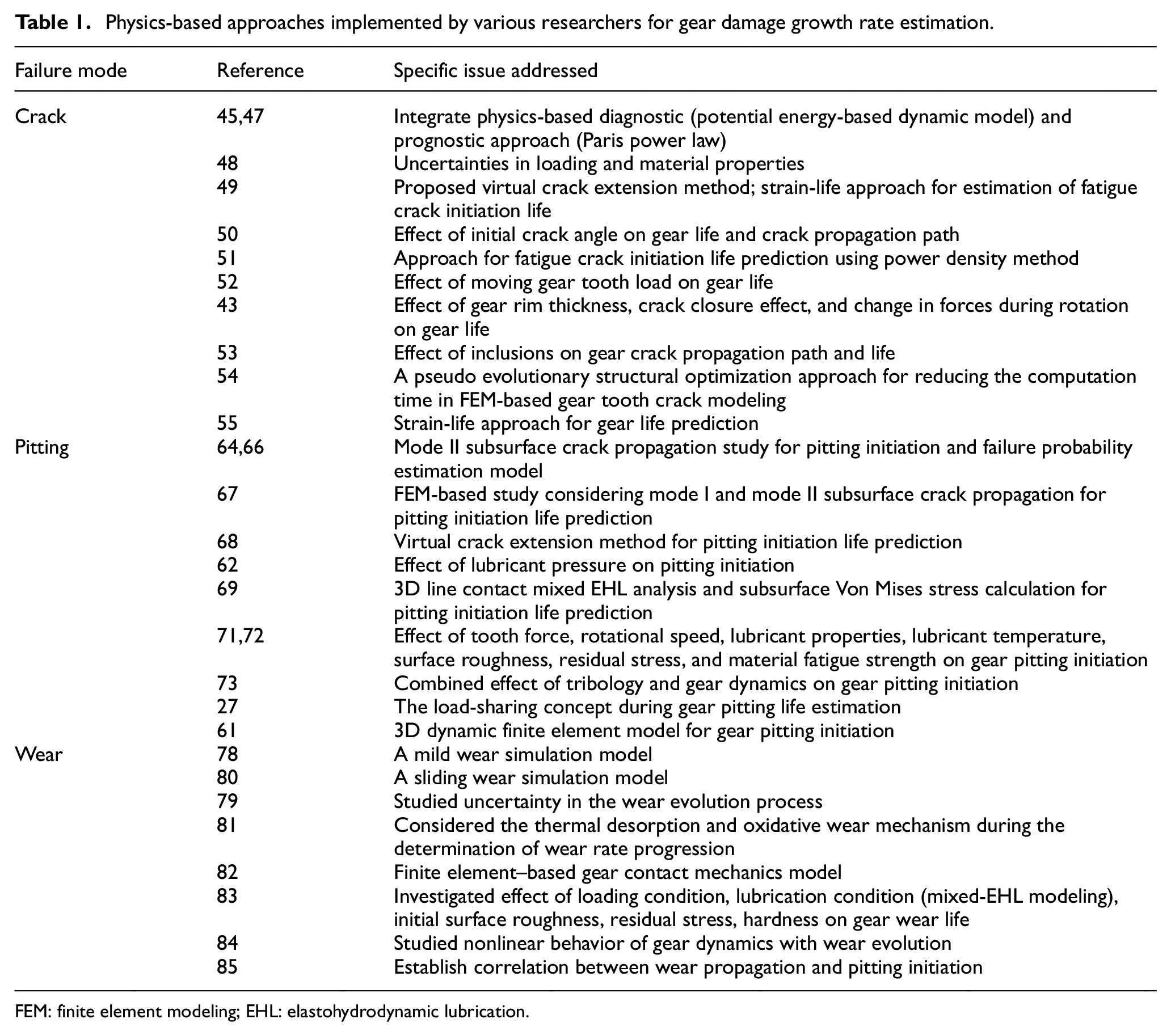
FEM: finite element modeling; EHL: elastohydrodynamic lubrication.

In summary, Figure 2 represents a typical physics-based framework for fault diagnostics and prognostics. The observed damage level and location can be modeled into the dynamic system model that can give the vibratory response using the dynamic model. This helps in the process of diagnostics based on a physics-based approach. Based on fault diagnostics information, the physics-based prognostic approaches can provide good prediction results if properly modeled. However, the physics-based prognostic approaches have a few major drawbacks that need to be addressed. First, much effort is required to estimate the fatigue model parameters, for example, $C$ and $m$ in equations (2) and (5) and $k$ in equation (7). In addition, the accuracy of the physics-based prognostic approaches depends on the exact estimate of the current health state of the gear. If the current health state is not accurately assessed, it may result in a higher error in the prediction of the evolution of the particular gear fault. Combinations of failure modes may sometimes appear in a practical situation, and the complexity of the physics-based approaches can be challenging in such scenarios.

Figure 2.

Physics-based framework for fault diagnostics and prognostics.

The physics-based prognostics model calculates the time to reach a future predefined threshold value of the damage area based on constant fatigue parameters, for example, $C$ and $m$ in equations (2) and (5) and $k$ in equation (7). However, constant parameters cannot model the stochastic nature of the damage growth on the gear tooth surface. In addition, the values of these constants derived from the quantification (measurement) of the damage area may be affected by process and measurement noise. Additional factors such as environmental condition, characteristic, and relationship between all the related parameters are difficult to model. All these factors make the prediction made by the mathematical or empirical model highly error-prone. Uncertainty and error in prediction can be reduced if the model parameters are updated based on the current health condition.

Parameters updating of the physics-based prognostic models

Due to the complexity of the mechanical systems, inherent uncertainty due to underlying modeling assumptions, process noise, and measurement noise, the prediction made by the physics-based prognostic models is always error-prone.¹⁶ The parameter updating approaches such as Kalman filter (KF), extended Kalman filter (EKF), linear Kalman filter (LKF), particle filter (PF) and so on help to overcome these uncertainties in the prognostic models. Table 2 lists some of the parameter updating approaches that can be used for updating the physics-based prognostics model parameter.

Table 2.

Model parameters updating approaches.

Reference	Approach
74,86	Least square
87,88	Linear Kalman filter
89 –98	Particle filter
99 –103	Extended Kalman filter

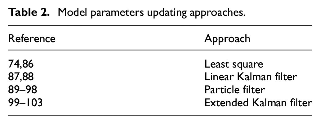
Most of these parameter updating approaches are based on the Bayesian inference. Using the Bayes theorem, these approaches estimate and update the model parameters in the form of probability density function (PDF)

p (Ø | D) = L (D | Ø) \times p (Ø)

(9)

where Ø is the vector of the unknown physical model parameters, $D$ is the vector of the observed damage data, $p (Ø | D)$ is the posterior PDF of Ø conditional on $D$ , $L (D | Ø)$ is the likelihood value of $D$ conditional on the given Ø, and $p (Ø)$ is the prior PDF of Ø. A Monte-Carlo simulation methodology is used to update the model parameters in these Bayesian inference-based approaches.^89–91 The state transition function $f$ and the measurement function $h$ are required for parameter updating. In general, the state transition function can be given as

x_{k} = f (x_{k - 1}, θ_{k}, v_{k})

(10)

where $x_{k}$ is the damage state, $k$ is the measurement cycle, $θ_{k}$ is the vector of model parameters, and $v_{k}$ is the process noise. For the measurement function $h$ , it is assumed that the $k th$ measurement $D_{k}$ is the same as $x_{k}$ with the inclusion of some measurement noise $w_{k} ~ N (0, σ)$ with standard deviation $σ$

D_{k} = h (x_{k}, w_{k})

(11)

For the implementation of the updating algorithms, it is assumed that the model parameters follow some distribution, that is, normal with their initially known mean and standard deviation given as

x_{0} ~ N (μ, std), Ø_{0} ~ N (μ, std)

(12)

Initially, based on an a priori known distribution in the parameters, $n$ samples of the parameters are drawn, which is $p (Ø)$ . The likelihood of the measurement data $L (D | Ø)$ is also assumed to follow some distribution. Now, the prior distribution $p (Ø)$ and the likelihood $L (D | Ø)$ are used to estimate the posterior distributions of the model parameters using equation (9). Finally, a resampling method is employed for duplicating the samples with high weight in the posterior distributions and eliminating the samples with low weight. After elimination, the mean of the posterior distribution of the model parameters can be considered as an updated physics-based model parameter value.

Data-driven approaches

The data-driven framework for fault diagnostics and prognostics is built based on the historical run to failure CM data. The key elements for a data-driven framework are suitable sensor selection and data acquisition, data processing, HIs construction for fault diagnostics, indicators processing/selection, fault classification, and fault prognostics. Broadly, a typical data-driven framework for fault diagnostics and prognostics is outlined in Figure 3.

Figure 3.

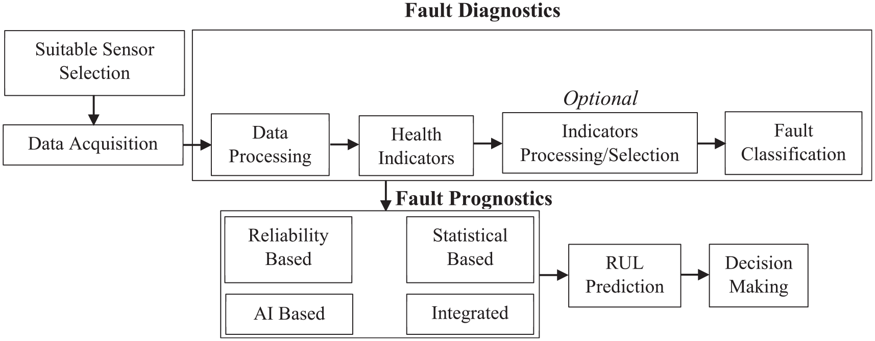
Data-driven framework for fault diagnostics and prognostics.

Sensor selection and data acquisition

Several sensors can be installed at various locations on the gearbox to monitor its condition. Typical sensors for monitoring the health of the gear include accelerometers for measuring vibration, acoustic emission (AE) sensor for measuring AE stress waves, wear debris sensor for measuring the amount of material removed on the gear tooth surface, a thermocouple for measuring oil temperature, sound microphone for measuring noise, torque sensor for measuring torque fluctuation, and so on. The sensor selection depends on the constraints such as accuracy, cost, location, size, frequency range, amplitude range, and working and environmental conditions. However, the most important parameter for the selection of a sensor is the ability of the sensor to effectively capture a small change in the gear tooth health condition. From the literature, it is observed that the vibration, AE, and wear debris sensor most effectively capture changes in gear tooth and mostly used for gear CM. Table 3 shows the pros and cons of these sensors used for gear CM. In general, as compared to other sensors for gear CM, it is observed that the vibration sensor signal contains most of the information related to the gear dynamics and is quite responsive to the most types of gear tooth degradation. The vibration sensor is also cost-effective and convenient to use. Hence, this work mainly emphasizes the data-driven framework based on vibration signal. The acquisition of the data from all the sensors is carried out using an appropriate data acquisition system. It converts the typical input analog signal from the sensors into a set of discrete digital values that can be further processed for extracting the HIs relating the gear health information. Using the changes in the gear pair dynamics as elaborated above, a number of HIs can be extracted for the gear fault diagnostics and are discussed in the next section.

Table 3.

Pros and cons of sensors used for gear condition monitoring.

Condition monitoring sensor	Pros	Cons
Vibration	Vibration signal can be better correlated with gear dynamicsResponsive to gear tooth degradationPossible to detect the type, location of the defect, and defective component in a gearboxEasily amenable to wireless capturing of the vibration signalCost-effective compared to wear debris and acoustic emission sensor	Expert knowledge is required for extracting the HIs from the signalThe signal may be affected by structural resonance and mechanical background noiseDirection dependent
Acoustic emission	Very good signal-to-noise ratioNot affected by the structural resonance and other kinds of noisesLargely independent of directionGood sensitivity to incipient fault	Compared to the vibration sensor, acquisition hardware and associated accessories are very costly for acoustic emission sensorNeed to acquire at a higher sampling rateExpert and domain knowledge is essential for better correlation of AE signal with gear dynamicsThe signal is significantly affected by electromagnetic interferenceSignal analysis needs high computational requirement compared to the vibration sensor
Wear debris	Easy to useExpert knowledge is not essential for signal analysisGives a strong correlation with physical damage on the gear tooth surface	Can’t be useful to detect all kind of fault, for example, crackHard to use in some gear applications where grease is used instead of oil for lubricationSensor data may be affected by the degradation of other mechanical components inside a gearboxExpensive compared to vibration and acoustic emission sensorUnable to distinguish between different kinds of failure modes

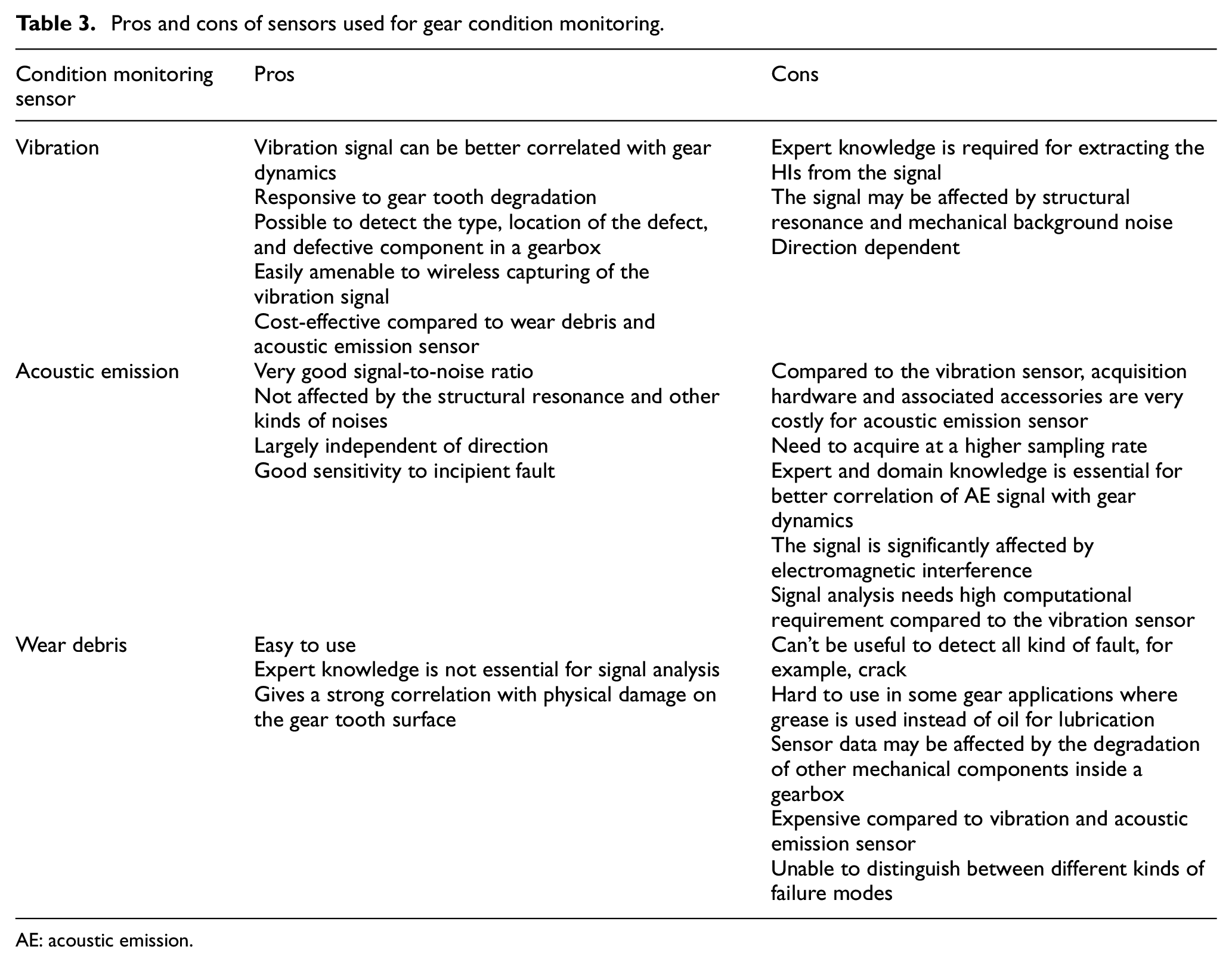
AE: acoustic emission.

Gear fault diagnostics

Gear fault diagnostics is a combination of sequential steps such as sensor data processing, HIs construction, HIs processing/selection, and gear fault type/severity classification. This stage is designed to generate a vector of HIs, which can be used to infer the current health status of a monitored system. The generation of an appropriate HI vector is typically application dependent and is one of the most important stages in a PHM framework. For a robust and more reliable correlation of the signal with the gear tooth condition, pre-processing of raw vibration data is usually necessary, which is discussed in the next section.

Data processing

The raw vibration signal generated in the gearbox has three main components (1) periodic components due to interactions between the pair(s) of gear teeth during meshing, (2) transient components due to short-duration impact because of tooth fault, and (3) broadband background noise.¹⁰⁴ In addition, the signal captured by the accelerometers over the gearbox housing is usually affected by the interference signal such as vibrations from shafts, bearings, and so on. The signal may also be contaminated by other disturbances such as electrical and electromagnetic.

One of the various ways in which various frequency components or a family of frequency components related to gear can be isolated/extracted from the raw vibration signal is the time synchronous averaging (TSA). The TSA approach allows separation of rotation speed synchronous components related to the gear of interest from other non-synchronous components, including the random broadband noise present in the raw vibration signal. In TSA, the raw vibration signal in the time domain is averaged over a large integer number of cycles synchronous with rotation of the particular gear shaft with the help of the tachometer sensor (reference) signal.^105,106 The noise and contribution of the signals from other machine components are significantly decreased using the TSA. Hence, the TSA time domain waveform is cleaner/purer compared to the original signal.¹⁰⁷ Some signal processing techniques are developed^108–110 in which tachometer signal information can be extracted from the vibration signal itself and hence TSA can also be performed without the need of a separate tachometer sensor.

The TSA signal gives direct visualization of the gear vibration signal and only localized tooth fault is easily discernible in the TSA signal, at least when fault becomes larger in size.²⁹ Many times, the TSA signal is further processed for diagnosing different kinds of gear faults which are difficult to diagnose using the bare TSA signal. Figure 4 shows different ways of processing the raw time domain data for diagnosing different kinds of gear faults.

Figure 4.

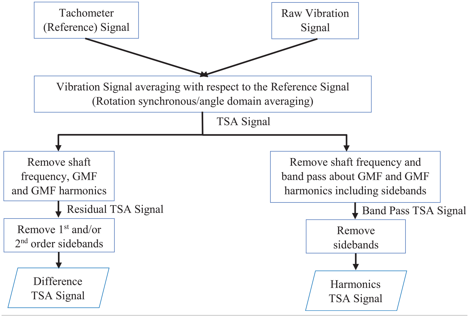
Data processing of raw vibration signal.

The residual TSA vibration signal is obtained by removing the shaft rotational speed components, GMF and GMF harmonics components from the original TSA signal. Thus, the residual TSA vibration signal only contains sideband information. As discussed earlier in section “Modulation-based models,” the increase in sidebands amplitude and families can be used for gear pitting detection. Hence, the residual TSA vibration signal, which only contains the sideband, is helpful for diagnosing the pitting fault.^32,105,111 For a tooth fault such as crack, it was observed that first- and/or second-order sidebands around each of the GMF harmonics produce large modulation effects that are not related to the local faults.¹¹² The researchers^113,114 have observed that gear tooth crack diagnostic-related information are more pronounced in the difference signal compared to the residual vibration signal. The band pass TSA signal is obtained by removing the rotational shaft frequency components and then band pass filtering of the remaining signal around the GMF and GMF harmonics. During filtering around each of the GMFs, up to fourth-order sidebands can be included in the filtered signal. If sidebands are removed from the band pass TSA, then the obtained signal is called a harmonics TSA signal. The harmonics TSA signal is helpful in diagnosing the presence of wear on the gear tooth surface. The processing of the raw vibration signal is reviewed in detail in previous studies.^21,23,24 For gear fault diagnostics, the most commonly used HIs extracted based on the processed/unprocessed vibration signal are discussed in the next section.

Construction of the HIs

The gear vibration signal is, in general, too complex to interpret directly and hence to map the degradation trend in the component health with the fault severity development, a HI is usually constructed.^115,116 Based on this HI, fault severity classification and prognostic approaches are implemented whose success depends heavily on the performance metrics of the HI, such as monotonicity, trendability, and robustness. This HI extraction process for the gear fault diagnostics can be done using processed/unprocessed vibration signal data in three different domains: time domain (TD), frequency domain (FD), and time-frequency domain (TFD). Different failure modes have different dynamics of initiation and rate of propagation. Hence, different indicators may need to be used to track different kinds of failure modes.³² Table 4 lists the most widely used HIs for different kinds of failure mode diagnosis in gear. A definition of these HIs is given in the subsequent sections.

Table 4.

Summary of the HIs used for diagnostics of various types of gear failure modes.

Type	Reference	Indicator name	Fault identified	Data processing
Time	117	RMS	General fault progression	Raw vibration signal
	21,117	Kurtosis	Tooth breakage, wear
	117	Crest factor (CF)	Localized tooth fault
	20,23	Energy operator	Scuffing, severe pitting
	118	Matched filtered RMS	Wear
	117,119	FM0	Tooth breakage and heavy distributed wear	TSA
	117,119 –121	NA4	Both single teeth pitting and multiple tooth pitting, progressing damage	Residual TSA
	23,117,122	NA4*	Progressing damage
	32	CCR	Pitting progression
	117,119 –121	FM4	Localized pitting or small crack on one or two teeth	Difference TSA
	114	M6A	Surface damage	Difference TSA
	117	Energy ratio	Heavy uniform wear	Difference and harmonics TSA
	123	NB4	Localized fault	Band pass TSA
Frequency	29	GMF harmonics amplitude	Wear	Raw vibration signal
	29	Sidebands amplitudes	Pitting	Raw vibration signal
	124	Side band ratio	Pitting	TSA signal
	125 –127	ALR	Crack
	34	ALR	Wear
	29,119,128	Cepstrum	For all kinds of fault	Raw vibration signal, TSA signal
	129,130	Spectral kurtosis	Pitting, crack	Residual signal, raw vibration signal
	30	Phase modulation	Crack	Band pass TSA signal
Time-frequency	131,132	NP4	For all kinds of fault	Raw vibration signal
	133 –146	Wavelet	For all kinds of fault
	147 –150	Empirical mode decomposition	For all kinds of fault
	151	CEEMD	For all kinds of fault
	152 –154	VMD	For all kinds of fault
	155	OEMD	For all kinds of fault
	156	Short-time Fourier transform (STFT)	Early-stage fault diagnostics	TSA
	157	Winger-Ville Distribution (WVD)	Early-stage fault diagnostics	TSA

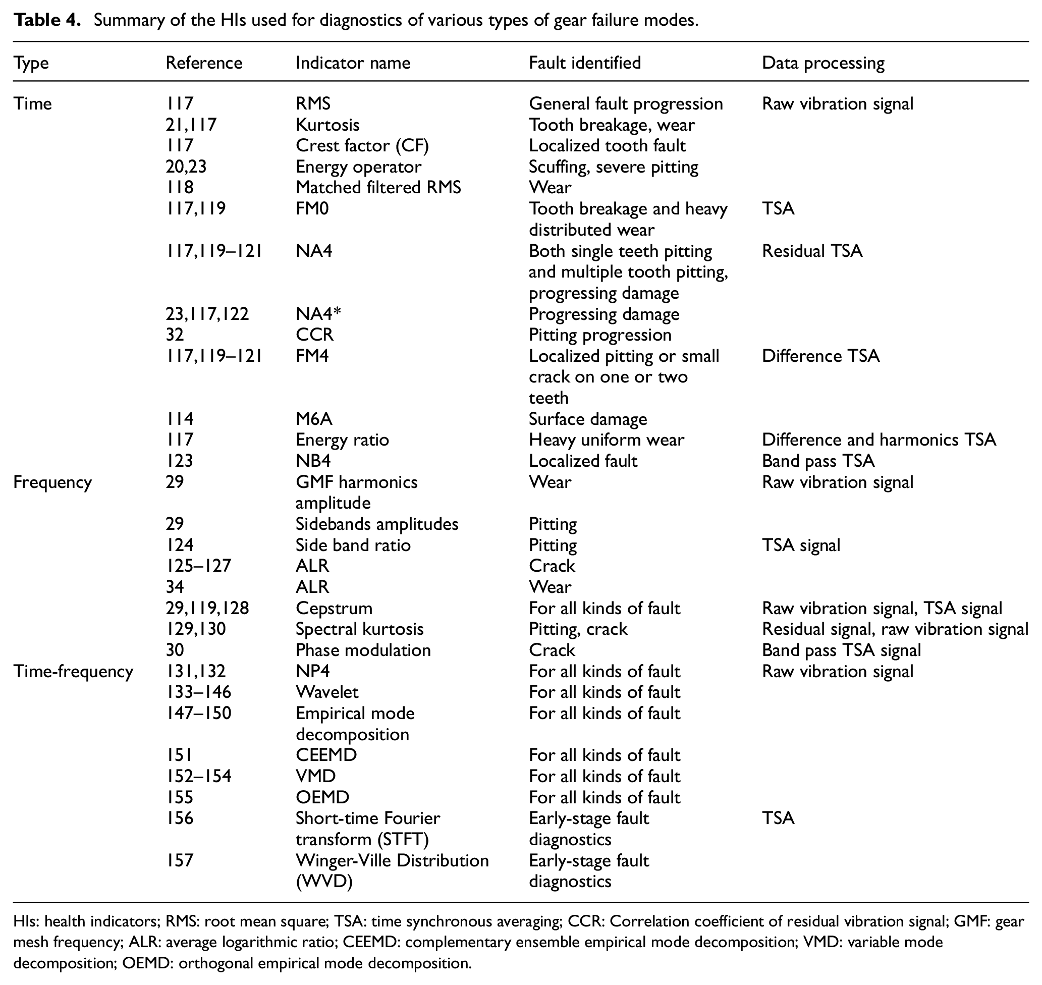
HIs: health indicators; RMS: root mean square; TSA: time synchronous averaging; CCR: Correlation coefficient of residual vibration signal; GMF: gear mesh frequency; ALR: average logarithmic ratio; CEEMD: complementary ensemble empirical mode decomposition; VMD: variable mode decomposition; OEMD: orthogonal empirical mode decomposition.

Time domain–based HIs

The TD-based HIs analyze the amplitude information or compare the vibration signal in a time series obtained in healthy and faulty stage for gear fault diagnostics. Based on the different types of signal pre-processing, various TD-based indicators can be extracted for gear fault diagnostics. The definition of the most widely used TD-based indicators is given in Table 5. The detailed description of many of these indicators can be seen in previous studies.^{20–25,117,158} In Table 5, $i$ is the data point number in the time record, $x_{i}$ represents $i th$ element of the raw vibration signal record, $d_{i}$ represents the $i th$ element of the difference vibration signal, $r_{i}$ represents the $i th$ element of the residual vibration signal, $j$ is the time record number in run ensemble, N represents the total number of data points/samples in a vibration signal, M is the current time record in a run ensemble, $\bar{x}$ is the mean of the raw vibration signal, $\bar{d}$ is the mean of the difference signal, $\bar{r}$ is the mean of the residual vibration signal, $f_{i}$ is the amplitude of the GMF or meshing harmonics, n is the number of GMF harmonics including GMF, and $var (r_{good})$ is the variance for a gear residual vibration signal in healthy condition.

Table 5.

Common TD-based indicators used for gear fault diagnostics.

Indicator name	Indicator definition
RMS	Although the mean square value is related to the overall signal energy, the indicator RMS is often used in practice to represent the vibration signal energy defined as the square root of the average of the sum of squares of N sample values of the signal. $RMS = \sqrt{\frac{1}{N} [\sum_{i = 1}^{N} {x_{i}}^{2}]}$
Kurtosis	The indicator Kurtosis is the normalized fourth moment of a signal and measures the peakedness of the signal. In a good condition, a gear vibration signal emulates a Gaussian distribution. The Kurtosis value of a Gaussian distribution is three and a value greater than three may indicate a gear in fault condition. For identification of gear faults such as tooth root cracks or large local spalls, Kurtosis is a good indicator. $Kurtosis = \frac{N \sum_{i = 1}^{N} {(x_{i} - \bar{x})}^{4}}{{(\sum_{i = 1}^{N} {(x_{i} - \bar{x})}^{2})}^{2}}$
CF	The indicator CF is the ratio of the maximum peak of the signal to the RMS value. For a localized tooth fault, the signal has sparse high amplitude peaks and this indicator is good for the identification of such faults. In general, for the fault in the initial stage, the CF shows higher sensitivity compared to either Kurtosis or RMS. $CF = \frac{{(x)}_{peak}}{{(x_{i})}_{rms}}$
Energyoperator	The indicator energy operator is calculated by modifying the input signal as follows $y_{i} = {x_{i}}^{2} - (x_{i - 1} \times x_{i + 1})$ For a sharp peak $x_{i - 1} & x_{i + 1}$ will be smaller than $x_{i}$ , $y_{i}$ will be improved with sharper peaks. The normalized kurtosis of the modified signal $y_{i}$ is termed as an energy operator. The impulse generated due to faults such as scuffing and severe pitting are more supported by this indicator.
FM0	The indicator FM0 is proposed by Stewart¹⁵⁹ and defined as the ratio of signal peak to peak value of the signal and the sum of amplitudes of meshing harmonics. $FM 0 = \frac{{(x)}_{peak - peak}}{\sum_{i = 1}^{n} (f_{i})}$ For a defect such as tooth breakage, the FM0 indicator value increases due to an increase in the peak to peak level of the signal. For defect such as distributed wear, although the peak to peak level of the signal remains constant, the modulation decreases the amplitude of the meshing harmonics components resulting in an increase in the FM0 level.¹¹⁹
FM4	For localized faults such as pitting or a small crack on one or more teeth, a series of peaks in the difference vibration signal increases.¹¹⁹ The kurtosis value calculated from this difference vibration signal can be a good indicator for diagnosing such localized fault, which is termed as FM4 $FM 4 = \frac{N \sum_{i = 1}^{N} {(d_{i} - \bar{d})}^{4}}{{(\sum_{i = 1}^{N} {(d_{i} - \bar{d})}^{2})}^{2}}$
NA4	The indicator FM4 was found to be insensitive to the distributed fault or less sensitive if damage progresses in both number and severity.¹¹⁷ Hence, a new indicator NA4 is proposed that is sensitive to progressive damage.¹²⁰ This indicator is calculated by the ratio of the fourth moment of a residual vibration signal to the square of the average variance of all previous data records in the run ensemble of the residual vibration signal. If gear damage spreads from one tooth to another tooth, the value of the average variance increases slowly compared to the numerator and allows the NA4 indicator to grow.²³ $NA 4 = \frac{N \sum_{i = 1}^{N} {(r_{i} - \bar{r})}^{4}}{{(\frac{1}{M} \sum_{j = 1}^{M} \frac{1}{N} (\sum_{i = 1}^{N} {(r_{i} - \bar{r})}^{2}))}^{2}}$
NB4	The NB4 indicator is similar to the NA4 indicator, with the only difference is that NB4 uses the quasi-normalized kurtosis of the envelope of the band pass TSA signal instead of the residual vibration signal. The signal envelope represents the AM due to transient variations in the loading. Transient load fluctuations caused by few damaged teeth can be seen in the signal envelope and this indicator quantifies those fluctuations.¹²³
M6A	The indicator M6A was developed for detecting the surface damage.¹¹⁴ Similar to the FM4 indicator, the only difference is that it uses the sixth-order moment normalized by the third power of the variance and is more sensitive to the peak in the difference signal. $M 6 A = \frac{N \sum_{i = 1}^{N} {(d_{i} - \bar{d})}^{6}}{{(\sum_{i = 1}^{N} {(d_{i} - \bar{d})}^{2})}^{3}}$
NA4*	The variance for the run ensemble keeps on increasing when the damage becomes distributed from localized. This results in a decrease in the NA4 indicator value in the advance pitting fault stage of the gear. Hence, the NA4 indicator is modified and termed as NA4, which continues to grow with the increase in the gear damage level. The NA4 indicator is a modified version of the NA4 in which normalizing is done by squared variance for gear in good condition. Minimum initial 30 data points can be considered for calculation of the variance of gear residual signal in good condition.^{23,117,122,123} $NA 4^{*} = \frac{N \sum_{i = 1}^{N} {(r_{i} - \bar{r})}^{4}}{{(var (r_{good}))}^{2}}$
EnergyRatio (ER)	The indicator ER is the ratio of RMS of difference TSA signal to RMS of the harmonics TSA vibration signal. This indicator is used for detecting the heavy uniform wear in gear.¹⁶⁰ The theory behind this indicator is that with wear progression, energy transfers from harmonics TSA signal to the difference TSA signal.¹¹⁷ $ER = \frac{{(RMS)}_{difference}}{{(RMS)}_{harmonics}}$

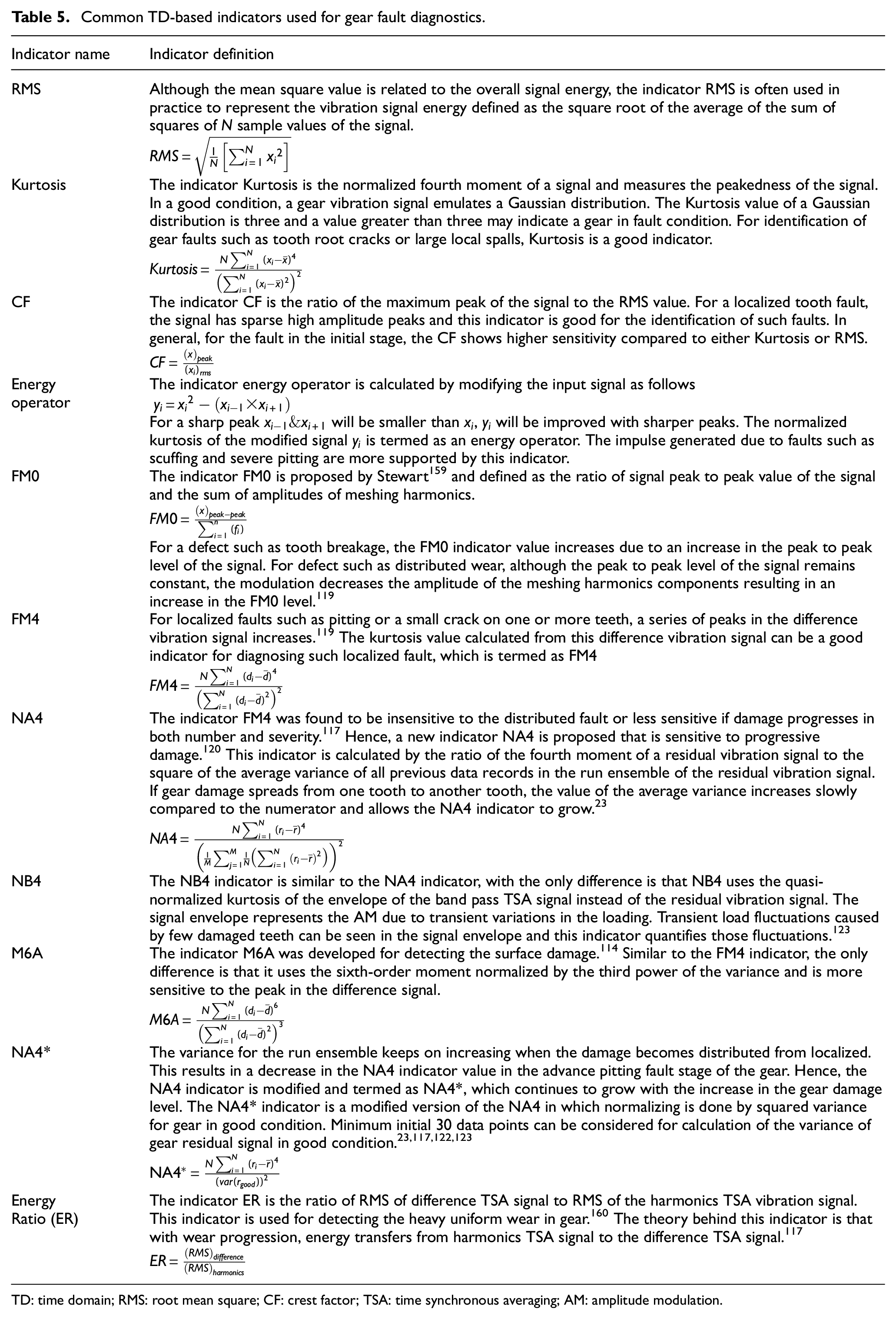
TD: time domain; RMS: root mean square; CF: crest factor; TSA: time synchronous averaging; AM: amplitude modulation.

Like kurtosis, the indicators FM4, NA4, and NB4 are dimensionless. For healthy gear conditions, the value of these indicators nearly three and a value of these indicators greater than three may indicate a faulty gear condition. A threshold may be defined for these indicators for the identification of different damage severity levels on the gear tooth surface.

In addition to the indicators discussed in Table 5, some other TD-based indicators were also extracted for gear fault diagnostics. For example, Mathew and Stecki¹¹⁸ developed an indicator named matched filtered RMS for detecting the wear progression. The matched filtered RMS is the logarithmic value of the average power ratio between the current health state vibration signal and a reference vibration signal. The sensitiveness of this indicator is found to be better than the traditional indicators such as RMS and peak. Wang¹⁶¹ used the resonance modulation technique for gear crack fault diagnostics. It is found that a crack in the gear tooth generates impacts that excite structural resonances. The residual TSA signal is band pass filtered around the structural resonance. The kurtosis of the envelope of the band pass filtered signal is found to be better than the kurtosis value of the raw signal for crack diagnostics. Kundu et al.³² proposed an indicator CCR for monitoring the natural pitting progression on the gear tooth surface. The indicator CCR compares the correlation of residual TSA vibration signal in the healthy/reference stage with the signal obtained in the current/pitted stage. The signal correlation is found to decrease with an increase in the pitting severity level on the gear tooth surface. In this study, the performance of the CCR indicator is compared with other indicators such as RMS, peak, CF, FM4, NA4, M6A, ER, and ALR in different pitting severity stages of the gear. It is shown that the indicator CCR value changes significantly in consecutive pitting stages of the gear compared to other indicators.

Frequency domain–based HIs

The indicators developed in this category are based on the changes in the frequency content of the vibration signals. In the FD, the mixture of different periodicities is easier to interpret compared to the TD.²⁹ Most of the gear fault diagnostic indicators developed based on this domain involve filtering the sidebands, GMF, or GMF harmonics from the raw/TSA signal and then analyzing them in the time domain using indicators discussed in the previous section. The relationship between the energy at different frequencies and gear damage is not well established. Hence, fewer studies are available for fault diagnostics based on the spectrum of the gear vibration signal. For example, Randall²⁹ observed that the presence of uniform tooth wear leads to an increase in the amplitude of the GMF harmonics amplitude and hence higher amplitude of the GMF harmonics can be used for detecting the uniform wear at an early stage. For defect such as pitting, increase in the sideband families and sideband amplitudes may indicate the presence of pitting on the gear tooth surface.²⁹

For defects such as crack, McFadden³⁰ observed that the phase modulation of the TSA signal band pass filtered around the dominating GMF harmonics can be used for early-stage gear crack diagnosis. The cracked tooth was detected by studying the phase angle and amplitude of the signal. Based on the sidebands information in the spectrum of the current stage and reference stage vibration signal, an indicator ALR has been used for detecting the crack on the spur gear tooth.^125–127

Combet and Gelman¹²⁴ proposed a side band ratio (SBR) indicator for differentiating the local tooth fault such as pitted gear from the healthy gear. The indicator SBR was calculated as the ratio of the sum of the amplitudes of sideband components of the envelope spectrum of a filtered signal around mesh harmonics to the measured power of the mesh harmonics. The first two harmonics were considered for pitting detection. Hu et al.³⁴ updated this indicator for monitoring the wear progression. The updated indicator was developed by the average logarithmic ratio of the current state SBR value to the reference state SBR value by considering all GMF harmonics in the signal. The logarithmic ratio was taken to deemphasize any substantial changes in the SBRs of any particular meshing harmonics.¹²⁵ Combet and Gelman¹²⁹ used the technique spectral kurtosis (SK) for the diagnosis of an early-stage pitting in gear. The SK technique was used to capture the small transients in the vibration signals. A similar technique was used by Barszcz and Randall¹³⁰ for crack fault identification in a wind turbine gear. Wang et al.¹⁶² describe the usage of the SK technique for gear fault diagnostics.

In addition to the spectrum analysis, some researchers^29,119,128 have used the cepstrum analysis for gear fault diagnostics, which detects the periodic structure in the spectrum. Cepstrum analysis is useful for separating overlapping side band families. The cepstrum represents a spectrum of the spectrum plot on a logarithmic scale. The cepstrum $C_{x} (τ)$ of a signal $x (t)$ can be defined as

C_{x} (τ) = {| F^{- 1} {\ln {| F {x (t)} |}^{2}} |}^{2}

(13)

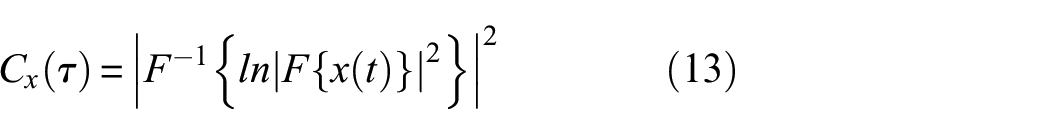
where $τ$ is the time-valued argument of the cepstrum (similar to $t$ for time series and $ω$ in spectrum).¹¹⁹

For surface wear diagnosis, Randall²⁹ observed that cepstrum analysis helps in distinguishing the family of harmonics with the family of equally spaced sidebands. Similarly, Ziaran and Darula¹²⁸ observed a larger change in harmonics amplitude of the cepstrum compared to the harmonics of the spectrum for a pitted gear. Sometimes cepstrum approach suppresses the useful fault diagnostic information available in the gear spectrum. Hence, it is advised that the cepstrum can be utilized to help in the understanding of the spectrum, instead of replacing it.²⁹

Many times, a local tooth fault such as initial pitting or crack generates small-amplitude short-duration transients in the vibration signal. In the normal spectrum, these changes may be submerged in the dominating components of the signal as all sections of the TD signal contribute to the normal Fourier spectrum. Hence, the global basis function does not effectively capture localized transient features. The Fourier spectrum is therefore insensitive to small localized temporal changes.¹⁵⁶ Hence, the FD-based HIs are not useful for the non-stationary vibration signal and fail to describe the evolution of the frequency content of the signal with time. It is therefore worthwhile to analyze the signal in TFD¹³⁴ in situations where short-duration transients are excited.

Time-frequency domain–based HIs

Multiple types of TD- and FD-based indicators are well established and explored for their effectiveness in gear fault diagnostics. However, it is reported that many times these techniques are unable to diagnose the fault in its early stages as these techniques are based on analysis of the signal assuming stationarity of the gear vibration signals. The periodic components present in the gear vibration signal show up readily in the frequency spectrum while the impulsive content is more appropriately descramble in TD. To capture both the information, the TFD analysis can be a good alternative.^21,133 The approaches such as short-time Fourier transform (STFT), wavelet transform (WT), empirical mode decomposition (EMD), and Wigner-Ville distribution (WVD) are commonly used TFD analysis approaches for gear fault diagnostics. The STFT represents the signal energy distribution over the frequency spectrum as it changes with time. It reflects changes in the short duration in the signal. Due to the application of a window function, the local damage on a tooth of the gear can be easily detected.¹⁵⁶ However, the approach has a disadvantage of a lack of simultaneous high resolution in both TD and FD.¹⁶³

WT that gives an improvement over the STFT technique is an adaptive multi-resolution analysis technique and is ideally suited to detect the non-stationary, non-periodic, and transient features in the vibration signal efficiently.¹³⁴ The WTs-based fault diagnostic methodologies may be categorized into a continuous wavelet transform (CWT), discrete wavelet transform (DWT), and wavelet packet transform (WPT). In CWT, the information on a series of wavelet coefficients at different scales is used for gear fault diagnosis. Polar wavelet maps were used by Meltzer and Dien¹³⁹ to improve the fault detection capability of a faulty gear operating under non-stationary rotating speeds. Various HIs were extracted using the wavelet coefficients of the CWT-based polar wavelet maps for the diagnostics. Similarly, Zhu et al.¹⁴⁰ mapped the wavelet coefficients into a polar diagram to enhance the periodic transients caused by gear faults such as pitting and crack. Morlet wavelet was used by Vernekar et al.¹³⁴ for diagnosing the missing tooth fault in the gear of an engine. The GMF amplitude in CWT was used to detect the presence of gear fault. Rafiee and Tse¹⁴¹ extracted the HI for diagnosing the various gear faults such as slight-worn, medium-worn, and broken teeth by approximating the autocorrelation function of the wavelet coefficients as a simple sinusoidal function. Zuo et al.¹⁴² used the WT to obtain multiple data series at different scales. These multiple data series were then used as an input to an independent component analysis (ICA) algorithm for the detection of an impulse generated due to broken tooth fault. Öztürk et al.¹⁴³ used the mean frequency of a scalogram to detect the presence of the pitting faults. Similarly, Wang et al.¹⁴⁴ proposed an HI from the amplitude of the wavelet coefficients of a CWT for a quantitative assessment of crack fault severity level under the varying operating conditions.

The CWT techniques are time-consuming and not suitable for large size of data set. It therefore becomes inconvenient for implementation of online fault diagnosis. The DWT is a fast computation version of the WTs. It is easy to implement and requires less computational resources in cost and time. In DWT, the signal is divided into approximation and detail coefficients depending on the level of decomposition. Saravanan and Ramachandran¹⁴⁵ used the DWT to represent all possible types of transients generated due to the presence of faults such as crack, wear, and broken tooth. Li et al.¹⁴⁶ used the DWT technique to denoise the raw vibration signal and diagnosed the gear faults such as crack, wear, and broken tooth, based on the autoregressive (AR) model and principal component analysis (PCA) approach. The WPT can be used as an alternative in applications wherein the DWT does not provide good fault diagnosis results. In WPT, the signal division takes place in each level of the approximated and detailed signals.¹³⁵ Hong et al.¹⁶⁴ identified the best sub-frequency band for classifying the condition such as normal, cracked, and broken teeth for a bevel gear based on the WPT technique. A detailed review of the application of different types of WT for fault diagnostics of rotating machinery elements such as bearings and gears is given in previous studies.^136–138

An alternative form of a TFD technique that is mostly used nowadays for fault diagnosis is an EMD. The EMD decomposes the non-stationary vibration signal into intrinsic mode functions (IMFs) that are nearly orthogonal. The IMFs represent the natural oscillatory mode embedded in the signal. Parey and colleagues^147,148 observed that the kurtosis value of the selected IMF was more sensitive to the incipient crack fault propagation compared to the kurtosis value of the raw original signal. Similarly, Li et al.¹⁴⁹ diagnosed a tooth crack in gear based on the marginal spectrum obtained using the EMD. Mode mixing is a major disadvantage of the EMD process, especially when the amplitude of the high-frequency component is smaller than the corresponding low-frequency component.^115,165 To counter the mode mixing and enable separation of the high-frequency component, Zhang et al.¹⁶⁶ used a frequency-modulated EMD technique. Zhao et al.¹⁵⁵ proposed an orthogonal empirical mode decomposition (OEMD) approach to reduce the effect of mode mixing, the influence of false frequency, and noise in the EMD approach. Liu et al.¹⁶⁷ used the ensemble empirical mode decomposition (EEMD) technique to counter the mode mixing problem. Although the EEMD technique has efficiently solved the mode-mixing problem, it takes a lot of time for decomposition. Zhao et al.¹⁵¹ proposed a complementary ensemble empirical mode decomposition (CEEMD) technique for gear fault diagnosis, which has less reconstruction error and is computationally more efficient compared to the EEMD technique. The poor performance of EEMD techniques is observed in the environment of strong noise present in the vibration signal. Recently, variable mode decomposition (VMD) technique is proposed for gear fault diagnosis due to high signal-to-noise ratio and better adaptability compared to EEMD.¹⁵² The selection of an optimum number of decomposition layers is one of the critical challenges during the implementation of the VMD technique. Algorithms such as particle swarm optimization (PSO),¹⁶⁸ grasshopper optimization,¹⁶⁹ ant colony optimization (ACO),¹⁷⁰ and artificial fish swarm optimization¹⁷¹ are used for optimizing the number of decomposition layers in the VMD technique. Lei et al.¹¹⁵ give a detailed review of EMD-based technique for fault diagnostics of rotating machinery.

Alternate time-frequency techniques are also used for gear fault diagnosis. For example, Wong¹⁵⁷ used the WVD technique for early-stage crack diagnosis in gear. Polyshchuk et al.¹³² proposed an indicator NP4 for gear fault detection based on WVD of the raw vibration signal. This indicator takes the kurtosis of the instantaneous power calculated using the WVD for gear fault diagnosis.^131,132 Feng et al.¹⁷² presented a review on the time-frequency domain-based HIs.

Processing/selection of the HIs

The accuracy of the classification and prognosis output of the models depend on the quality and sensitivity of indicators utilized to evaluate the condition of the faults. The HI processing step is optional while implementing the data-driven framework since its implementation depends on the correlation of the HI space with actual damage on the gear tooth surface. Figure 5 shows different ways of processing/selecting the HI space.

Figure 5.

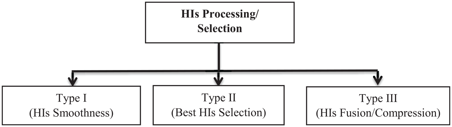
The HIs processing/selection for prognosis/classification model.

HIs smoothness

The HI value extracted from the vibration signal exhibits fluctuations with time. This variation is usually observed due to inherent complexity in the correlation between physical damage level and the corresponding HI value as well as due to the unpredictable balance between self-healing of the damage area and subsequent secondary degradation from primary damage sources. In some cases, there are other unexplained practical reasons. The actual measured data also has an inherent measurement noise. To avoid/reduce these fluctuations, the HI value is smoothened before it is used. For example, Tian and Zuo¹⁷³ smoothened the RMS-based HI using the Weibull hazard rate function for gear RUL prediction. A moving average method was used by Shao et al.¹⁷⁴ for reducing the fluctuations in the RMS-based HI value obtained from the vibration signal. For better fitting, some researchers have used the logarithm of HIs.^175–177 The main advantage of the indicator smoothness step is that it helps in removing the outliers present in the HI values and hence helps in improving the accuracy of prediction.

Best HIs selection

Most of the existing gear tooth fault diagnostic HIs are not equally sensitive at different damage levels. Some indicators are sensitive for the early-stage fault diagnostic and some are more sensitive for advanced stage gear fault diagnostic. The performance of an indicator depends on the fault characteristics, that is, type and location of the damage and whether the damage is distributed or localized.¹⁷⁸ Hence, the researchers usually extracted multiple indicators that are either sensitive in the early stage of gear fault or in the advanced stage of the gear fault. However, if all these indicators are used as inputs in the development of an RUL prediction or classification model, there is a strong probability that this input data may tend to describe the random error or noise apart from an underlying relationship. This is called overfitting of the model and in such cases, the performance of the model may be good during training but is likely to be significantly worse during testing. In addition to the effect on the performance, a large HI space increases the model learning time. Generally, two types of approaches are used to reduce the HI space dimensionality. The first approach involves the generation of a new HI with a lower dimension from the extracted HI space. This is done with the help of dimensionality reduction techniques that are discussed in section “Processing/selection of the HIs.” The second approach involves the elimination of the non-sensitive HIs from the HI space based on certain benchmarks that are discussed below.

In general, the indicators used for prognosis and classification should have the following three characteristics:^8,179

Monotonicity: represents an overall positive or negative trend in time.

Robustness: reflects the tolerance of the HI to outliers.

Trendability/correlation: the correlation of the entire history of the evolution of the HI with the fault progression.¹⁸⁰

The mathematical formulation of the metrics quantifying the characteristics described above can be found in Kundu et al.³² and Zhang et al.¹⁷⁹ In addition to these characteristics, other characteristics such as sensitivity and early detection for the HI can also be investigated. These characteristics of fault diagnostics are investigated by Shakya et al.¹⁸¹ for comparing the performance of various HIs. Instead of using a separate HI selection methodology, some prognosis models such as general log-linear Weibull (GLLW)^98,116 and random forest (RF)^105,182,183 have an inbuilt best HI selection capability. In the GLLW model, the backward stepwise regression procedure is followed for eliminating the least significant HIs and re-estimating the model parameters. This model provides statistical information in the form of p-values. The higher p-value (usually more than 0.05) indicates a poorer fit for the model. In addition, the RF approach that can be used for both classification and prognostics has the inbuilt best HI selection capability.

Other methods for best HI selection include Taguchi’s method used in Alkhadafe et al.¹⁸⁴ for classification of fault into the slight, moderate, and severe category in gear. The distance evaluation criterion for best indicator selection has been used in previous studies,^{167,175,178,185} whereas Lei et al.¹⁸⁶ and Cerrada et al.¹⁸⁷ used the genetic algorithm (GA) for best HI space selection. Shakya et al.¹⁸⁸ explored the use of Mahalanobis–Taguchi–Gram–Schmidt method and used gain values to remove/select appropriate indicators before the indicator fusion process. HIs processing/selection techniques discussed above can be implemented individually or together for improvement in the classification/prognosis accuracy, depending on the problem in hand.

HIs fusion/compression

Another way for HI space selection is to fuse all the indicators in such a way that it reduces the dimensionality of the extracted indicator space and at the same time retains the sensitivity or variability of all the indicators. Algorithms such as PCA,^{107,189–195} ICA,¹⁹¹ and Mahalanobis distance (MD)¹⁹⁶ are widely used for indicator fusion/compression.

Fault classification

Based on the identified HI space, the fault classification approaches classify different classes of faults in gear such as wear, pitting, crack, and tooth chipping. In addition, for a particular fault type such as pitting, the classification approaches can be used to classify the severity or the state of the gear pitting condition such as initial pitting, medium pitting, and severe pitting. The classification approaches separate the different fault classes based on some statistical criteria or hyper plane construction. Input from this step is very important while developing a prognosis model. For each type of failure mode, the evolution/trend of a particular fault indicator may be different. Hence, usually, a different prognosis model may need to be developed for each kind of failure in the component. Table 6 summarizes various classification approaches used for gear fault classification. Some of the most widely used approaches are discussed in the following subsection.

Table 6.

Fault classification models implemented by various researchers for gear fault severity classification.

Reference	Classification algorithm	Type of faults	Type of gear	HIs (HI processing techniques)
145	Neural network	Crack, wear, and tooth breakage	Bevel	Wavelet
184		Tooth breakage severity	Helical	A total of 25 TD-, FD-, and TFD-based HIs (Taguchi’s)
197		Tooth breakage, pitting, crack, and wear	Planetary	A total of eight TD- and FD-based HIs
198		Slightly worn, medium worn, and tooth breakage	Spur	Wavelet
199		Worn, broken, and missing tooth	Bevel	EMD
200	Fuzzy rule	Broken and worn tooth	Spur	Decision tree
201	Neuro-fuzzy	Crack and chipped tooth	Spur	Wavelet, beta kurtosis, phase modulation
202		Crack and chipped tooth	Spur	Wavelet, beta kurtosis, phase modulation
203		Crack, scoring, and pitting	Spur	Wavelet, beta kurtosis, phase modulation
204	SVM	Pitting of different severity level (slight, medium, and severe)	Planetary	A total of 34 TD- and FD-based HIs (feature ranking)
189		Spot damaged and pitted gear	Spur	Amplitude ratios of the frequency band (PCA)
107		Pitting of different severity level	Spur	RMS, peak, average signal CC, kurtosis, skewness, % energy of frequency band (PCA)
166		Crack and tooth breakage	Compound	% Energy of IMF of EMD
205		Missing tooth and chipping	Spur	Bee colony
167	RVM (Ant Colony)	Worn, broken, missing, chipped, pitted	Bevel	EEMD (distance evaluation criteria)
206	SVM and ANN	Pitting	Spur	GA
207		Tooth break, crack, and face wear	Bevel	Wavelet (decision tree)
208	SVM and KNN	Crack and missing tooth	Planetary	A total of 136 TD- and FD-based HIs (feature ranking)
209	LDA and SVM	Pitting of different severity level	Planetary	A total of 34 TD- and FD-based HIs (feature ranking)
210	Ordinal ranking	Pitting of different severity level	Planetary	A total of 34 TD- and FD-based HIs (correlation coefficient)
149	Euclidean distance	Crack of different severity level	Compound	EMD
186	Multiple classifier (MLPNN, RBFNN, KNN)	Chipped and missing tooth	Spur	A total of 29 TD-, FD-, and TFD-based HIs (GA)
211	KNN	Crack	Spur	A total of 25 TD- and FD-based HIs (weighting technique and Euclidean distance)
195	KNN	Crack	Spur	WPT (PCA)
212	Random forest	Crack, spall, and tooth breakage	Not specified	A total of 29 TD- and FD-based indicators
187		Pitting, wear, tooth breakage, and misaligned gear	Spur	A total of 39 TD-, FD-, and TFD-based indicators (GA)
213	Deep learning	Wear, pitting, and broken tooth	Spur	Mean, standard deviation, skewness, kurtosis in TD; RMS in FD
214		Crack severities	Spur	Time-frequency spectra
215		Wear, pitting, and broken tooth	Spur	Mean, standard deviation, skewness, kurtosis in TD; RMS in FD
216		Chipped and broken tooth	Spur	A total of 45 TD-, FD-, and TFD-based indicators
217		Chipped, worn, and broken tooth	Spur and helical	A total of 27 TD-, FD-, and TFD-based indicators
218		Pitting, chipped, crack, and missing tooth	Planetary	Frequency spectrum
219		Crack, broken tooth, and wear	Spur	Wavelet signal
220		Pitting, worn, and crack	Planetary	TD-, FD-, and TFD-based indicators
221		Wear, pitting, broken tooth, and chafing	Spur	TD- and FD-based indicators
222		Crack and missing tooth	Spur	Time-frequency plot
223		Tooth breakage	Helical	Raw vibration signal
224		Pitting, broken tooth, and wear	Not specified	Frequency spectrum

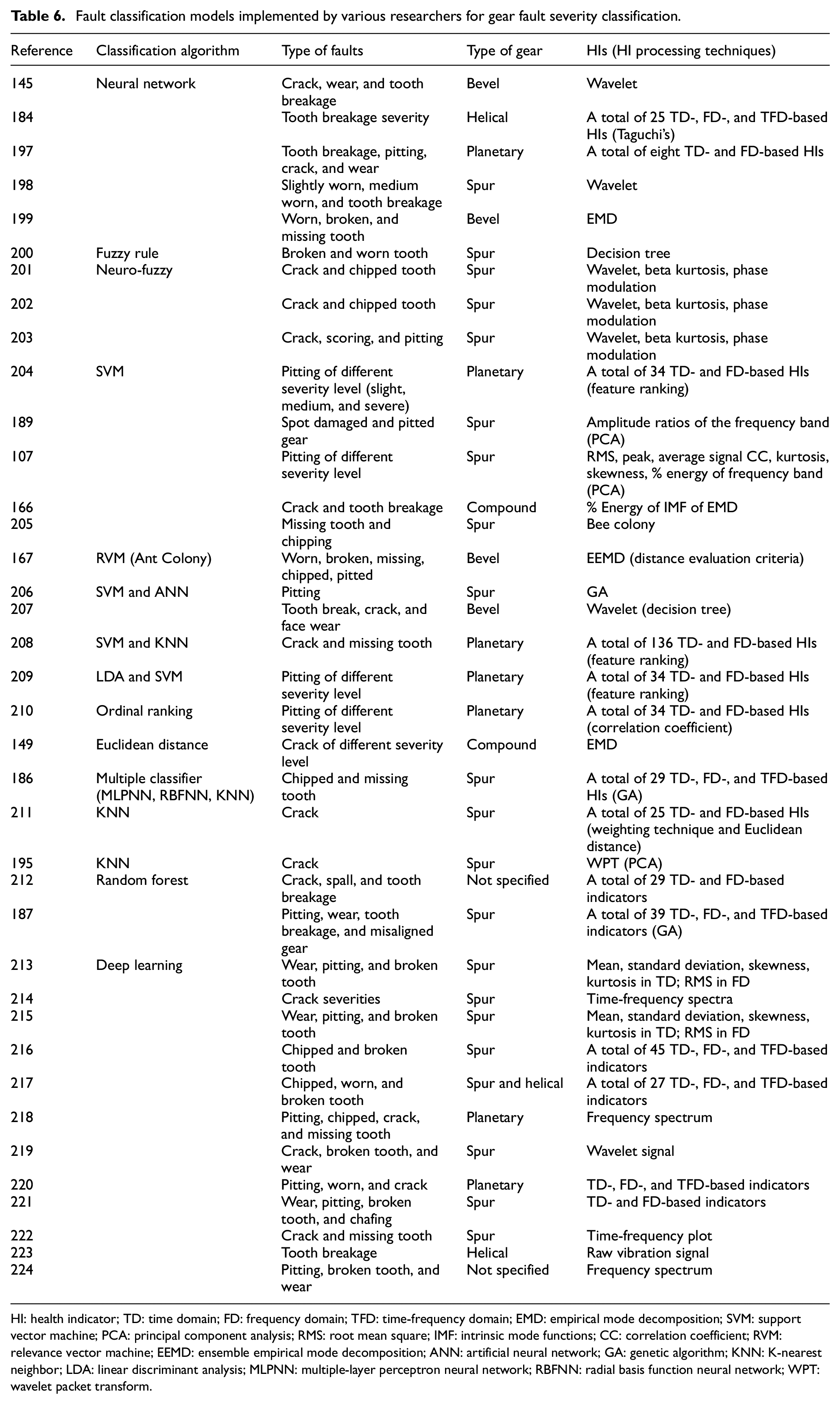
HI: health indicator; TD: time domain; FD: frequency domain; TFD: time-frequency domain; EMD: empirical mode decomposition; SVM: support vector machine; PCA: principal component analysis; RMS: root mean square; IMF: intrinsic mode functions; CC: correlation coefficient; RVM: relevance vector machine; EEMD: ensemble empirical mode decomposition; ANN: artificial neural network; GA: genetic algorithm; KNN: K-nearest neighbor; LDA: linear discriminant analysis; MLPNN: multiple-layer perceptron neural network; RBFNN: radial basis function neural network; WPT: wavelet packet transform.

Neural network

The idea of an artificial neural network (ANN) is inspired by the biological nervous system and is the most popular methodology used for classification problems due to its prediction capability. The ANN model learns from the training in a way similar to the biological neural network learns from the experience.²²⁵ Different structures and types of ANN models are trained by various researchers for gear fault severity classification. For example, Saravanan and Ramachandran¹⁴⁵ used the back propagation neural network approach to identify different kinds of faults such as crack, wear, and tooth breakage in a bevel gear. Wavelet-based HIs were extracted from the wavelet coefficients obtained using the Daubechies wavelets “db1” to “db15.” The HIs generated from the wavelet that gives the highest potential to identify different types of faults in gear is used as inputs for classifying a different kind of fault in gear. The accuracy of the ANN model was tested with the number of neurons between 2 and 30. The number that resulted in the minimum classification error was selected for building the structure of the ANN for fault classification. Alkhadafe et al.¹⁸⁴ used multiple sensors such as vibration, acoustic, speed, and torque for classification of the pitting fault severity into initial, medium, and severe pitting in a helical gear. Various TD-, FD-, and TFD-based HIs were extracted from the sensor signals. Taguchi’s method was used to select the best indicators that are sensitive to different fault types in gear and are then used as inputs to the neural network. Two types of neural networks, namely, back propagation and radial basis, were used in this study for fault severity classification. Rafiee et al.¹⁹⁸ used the multi-layer perceptron neural network for classifying the gear faults such as slight-worn, medium-worn, and broken-tooth. A self-organized map (SOM) neural network was presented by Cheng et al.¹⁹⁹ for identifying the gear faults such as a worn, broken, and missing tooth.

The neural network-based models have two critical disadvantages. First, it is difficult to determine the optimum network structure and number of nodes.^226,227 Second, the neural network training algorithms may not give the same results for each run during training with the same input, output, and model structure.²²⁸ To overcome the first disadvantage, researchers have attempted some optimization algorithms for finding out the optimum number of hidden layers and neurons in the network. For example, Samanta²⁰⁶ optimized the number of nodes in the hidden layer of an ANN model using GA.

Fuzzy rule

In the fuzzy rule-based approaches, the rule set is usually learned from the knowledge of the expert or prior system knowledge for fault classification. Jolandan et al.²⁰⁰ used a fuzzy-based approach for the classification of faults such as a broken and worn tooth. For developing the rules, the decisions tree approach was used. A major issue with the fuzzy approaches is the correctness of the rules developed from the expert knowledge or requirement of a separate algorithm for defining the rules. Hence, some researchers^201–203 integrate the fuzzy approaches with the neural network for automatically defining the rules. The integration overcomes the interpretability issue of the ANN and rule defining issue of the fuzzy approach.

Support vector machine

The support vector machine (SVM) is a nonlinear approximation approach and can give better classification accuracy even with a small sample size.²²⁹ It maps the input data x in a nonlinear fashion into a higher-dimensional HI space via kernel functions.^178,191 Each instance in the input HI space is assigned with a class label of +1 or −1. For example, if $x_{i}$ is the input vector and $d_{i}$ is the desired value, then the SVM considers the data set as $(x_{1}, d_{1})$ , $(x_{2}, d_{2})$ , …, $(x_{n}, d_{n})$ , where, $d_{i} \in {- 1, + 1}$ . The SVM classifies the dataset by constructing a hyper plane and attempts to find the optimum boundary in such a way that the margin between two classes is maximum.²³⁰ The nearest data point used for determining the margin is called support vectors.²³¹

A basic SVM classifier can only be used for two-class classification problems. For solving the multi-class classification problems using SVM, many classifier architectures such as one-against-one, one-against-all, and direct acyclic graph have been developed.^189,232,233 Qu et al.²⁰⁴ used the multi-class SVM approach for the classification of different levels of pitting severity (initial, medium, and severe pitting) in a planetary gear. A total of 134 TD- and FD-based HIs were extracted from the raw vibration signals. Based on this HI space, an SVM classifier was built and different damage severity levels were classified. Zhang et al.¹⁶⁶ observed that the energy distribution of the IMF extracted using the EMD process can be used to recognize the dynamic state and fault type of gear. With the multi-class SVM approach, gear health stages such as healthy, crack, and broken teeth were identified. For multi-class classification, Liu et al.¹⁶⁷ proposed a Kernel-based approach similar to the SVM called relevance vector machine (RVM) and obtained better accuracy compared to that from the SVM.

As discussed earlier, the accuracy of the SVM-based approaches depends on the values of the kernel parameters and there is no precise basis to determine suitable kernel parameters for a given problem.²³⁴ Some optimization algorithms are required to find the optimum kernel parameters. Liu et al.¹⁶⁷ obtained the optimum kernel parameters using the ACO algorithm. Higher accuracy was observed with the ACO-RVM approach compared to that from the RVM approach. In this work, 14 TD-based HIs and 13 FD-based HIs were extracted from the first three IMFs extracted from the EEMD process.²³⁵ Based on the distance evaluation criteria, dominant HIs were selected for the HI space to the RVM model for improving the fault classification accuracy. Similarly, Samanta²⁰⁶ used the GA for optimizing the SVM kernel parameters. The SVM classifier is less influenced by the HI space dimensionality and is less prone to the overfitting problems as observed with the neural networks.²³⁶ Hence, some researchers^206,207 have observed that the SVM outperforms the ANN-based models in terms of classification accuracy.

Random forest

Recently, RF methodology is used by various researchers^{182,183,187,212} for fault severity level classification. The RF methodology has fewer hyper-parameters and easy to interpret. Compared to the algorithms such as ANN and SVM, it provides a higher or at least comparable classification accuracy. The RF is an ensemble learning methodology that integrates the multiple weak and diverse decision tree classifiers and reaches a final decision by majority of votes from the multiple decision trees.²¹² Han et al.²¹² compare the performance of RF, ANN, and SVM models for classifying faults such as spalling, crack, and broken tooth. Compared to the SVM and ANN algorithms, the performance of the RF algorithm was found superior, especially when the number of training samples was limited and noise in the signal is high. Cerrada et al.¹⁸⁷ used the RF algorithm with the integration of GA for classification of gear faults such as pitting, wear, broken tooth, and misaligned gear. In this work, many TD-, FD-, and TFD-based indicators were extracted from the raw vibration signal and the GA was applied on these indicators for selecting the best indicators. The best indicators were used as inputs to the RF model for gear faults classification. The RF methodology has an inbuilt best HI selection capability. The separate GA used in the above work for selecting the best HIs is not required if RF is used as a fault classification model. The best HI selection capability inbuilt in the RF model is demonstrated in previous studies.^182,183

K-nearest neighbor

The K-nearest neighbor (KNN) is a type of instance-based learning algorithm that works based on the principle that the instances within a dataset lie in close proximity to the other instances with similar properties.²³⁷ The KNN is more stable and has a good classification performance compared to other algorithms such as ANN and SVM. For example, Wang¹⁹⁵ identified five crack severity levels on gear tooth using the KNN algorithm based on HIs extracted from WPT. The highest classification accuracy was observed with the KNN algorithm compared to algorithms such as linear discriminant analysis (LDA), quadratic discriminant analysis (QDA), classification and regression tree (CART), and Naïve Bayes classifier (NBC). Similarly, Liu et al.²⁰⁸ observed the comparable performance of the KNN with the SVM algorithm for the identification of crack and missing teeth in a planetary gear train.

Deep learning

The performance of the conventional machine learning approaches depends on the sensitivity of the HI value to the fault progression. The extraction of appropriate HI requires domain knowledge and understanding of signal processing techniques. In recent years, deep learning-based neural network models have become popular for fault classification. They reduce the manual processing and analysis of the data. The deep learning models learn features from the raw data. Their deep architecture contains many layers of nonlinear data processing units.²³⁸ Each layer learns a higher level of raw vibration data representation from the output of its preceding layer. Hence, deep learning models automatically extract multiple complex features/indicators from the raw vibration data without the use of human expertise, domain knowledge, and signal processing techniques.²³⁹ Different types of deep learning architectures such as convolution neural network (CNN),^{214–216,219,222} stacked auto encoder (SAE),^{218,220,224,240} deep belief network (DBN),^213,223,241 and deep Boltzmann machine (DBM)²²¹ are applied for gear faults classification. Some architectures were applied to the HIs extracted from the raw vibration signal,^{182,184–186,189,190} whereas some architectures were applied to the raw vibration data in the time domain,^{223,242–244} frequency domain,^218,224 and time-frequency domain.^214,219,222

For example, a local-global deep neural network (LGDNN) was proposed by Zhao and Jia²²³ for diagnosing different kinds of bearing faults and different fault severity levels for gear using raw vibration data in the time domain. In the local layer of the LGDNN model, an improved convolutional deep belief network (CDBN) based on the Fisher parameter optimization criterion (called Fisher-CDBN) is used to efficiently extract local discriminant information from the raw vibration data. In the secondary global layer of the network, the kernel PCA is used to reduce the redundancy attribute of the data. Jia et al.²¹⁸ used an auto encoder-based deep neural network (DNN) model for classifying different kinds of gear faults using frequency spectra of the machinery. Different types of faults such as pitting on sun gear, cracked sun gear, chipped planetary gear in the first stage, chipped sun gear, a missing tooth sun gear in the second stage, and an inner race bearing fault of planetary gear in the first stage was classified in this work. Wang et al.²¹⁴ used the CNN model for classification of gear fault severity levels such as slight crack, medium crack, and broken teeth. The time sequences in this work were converted to time-frequency images by wavelet analysis. The CNN model learns the underlying features in the signal from the time-frequency domain spectral images and performs fault classification.

The conventional classification algorithms are suitable for one operating condition. If the operating conditions change for the system, then the historical data for the changed value of the operating condition is required and the model needs to be retrained to accommodate the additional operating condition. This issue is overcome by deep transfer learning approaches developed recently. For example, Li et al.²⁴³ proposed a deep transfer learning network (DTLN) to diagnose different pitting severity levels. The parameters of the DTLN model in this work were optimized using PSO algorithm. Han et al.²⁴⁴ used the CNN model for diagnosing multiple fault types in the gear, bearing and shaft for a compound gearbox. In the source domain, the CNN model was trained on a large dataset to learn hierarchical features from the raw vibration data. The architecture and weights of this CNN model in the source domain were fine-tuned for classifying the fault severity level/types in the target domain (for different operating conditions). Different types of architectures developed in the deep transfer learning category for gear fault diagnosis can be referred in previous studies.^242,245,246

Compared to conventional machine learning approaches, designing a deep learning architecture is still a challenge. The deep learning model has so many hyper-parameters and each hyper-parameter has a substantial effect on the model performance. More standard methods need to develop for the selection of the optimal hyper-parameters for a particular fault diagnosis problem.²³⁹ A detailed description of deep learning–based models for machinery fault diagnosis can be seen in previous studies.^{239,247–249}

Miscellaneous

In addition to the major approaches discussed above, other approaches have also been tried for gear fault classification. For example, Cheng et al.²⁵⁰ proposed a gray relational analysis approach for the identification of the different level of pitting severity in gears. In this work, the best HIs were selected based on their correlation to the damage severity level. Based on the selected best HIs, the relational analysis of gear in the healthy stage is carried out with the gear in different pitting severity levels. Zhao et al.²¹⁰ classified the artificially created pitting surface damage using an ordinal ranking/classification methodology. A total of 63 TD- and FD-based HIs were extracted from each vibration sensor data. Vibration sensors at four different positions were used for health monitoring of the gear and hence total 252 HIs were available for gear pitting severity level classification. The correlation coefficient of each HI vector with the pitting severity level is estimated and indicators with high correlation coefficient value were considered for pitting severity classification.

The detailed mathematical and graphical description of classifier models for machinery fault diagnosis is given in Liu et al.²³⁷

Fault prognostics

In contrast to the wide variety of fault diagnostic approaches available for gears, fault prognostic approaches are limited in the open literature. This may be due to the non-availability of the run to failure data for gears. The data-driven methodologies used for gear fault prognostics are tabulated in Table 7. A detailed description of each of these RUL prediction methodologies is not given here, as many reviews^{9,11–13,19,237,248,251–255} are already available on general data-driven prognostic methodologies and hence some of the common RUL prediction methodologies that are used specifically for gears are discussed in this section.

Table 7.

Data-driven prognostic models implemented by various researchers for gear RUL prediction.

Reference	Prognostics model	Type of fault	Gear type	HIs (HI processing techniques)
256	ANN	Wear	Compound	Sideband index
173		Broken tooth	Compound	RMS
257	Neuro-fuzzy	Pitting	Spur	CWT
258	Deep neural network	Wear	Bevel	RMS, ER RMS, FM0, narrowband kurtosis, AM kurtosis, and FM RMS
259	ANFIS and SVR	Worn, chipped, crack, and pitting	Spur	CWT, normalized kurtosis, and shaft frequency spectrum
260	ANFIS and NARX	Not specified	Planetary	Transient analysis algorithm and wavelet denoising
261	PF	Pitting	Bevel	Cholesky decomposition-based whitening transform
262		Wear	Compound	Special frequency band energy data
263		Not specified	Compound	Specific band energy
264	ANFIS and PF (current signature)	Wear	Compound	PSD of the current signature
265	State space	Wear	Planetary	Backlash, vibration, and wear
266		Wear	Spur	PSD amplitude at GMF
267		Wear	Helical compound	Not given
268	Stochastic filtering	Not specified	Not specified	RMS, CF, clearance factor, and shape factor
269	HMM	Wear	Spur	WT
270	HMM and PF	Not specified	Helical	HI developed using HMM
191	Proportional hazard model, SVR, and exponential extrapolation	Wear	Spur	TD-, FD-, and TFD-based indicators (ICA)
105	RFR	Pitting	Spur	CCR (MD)

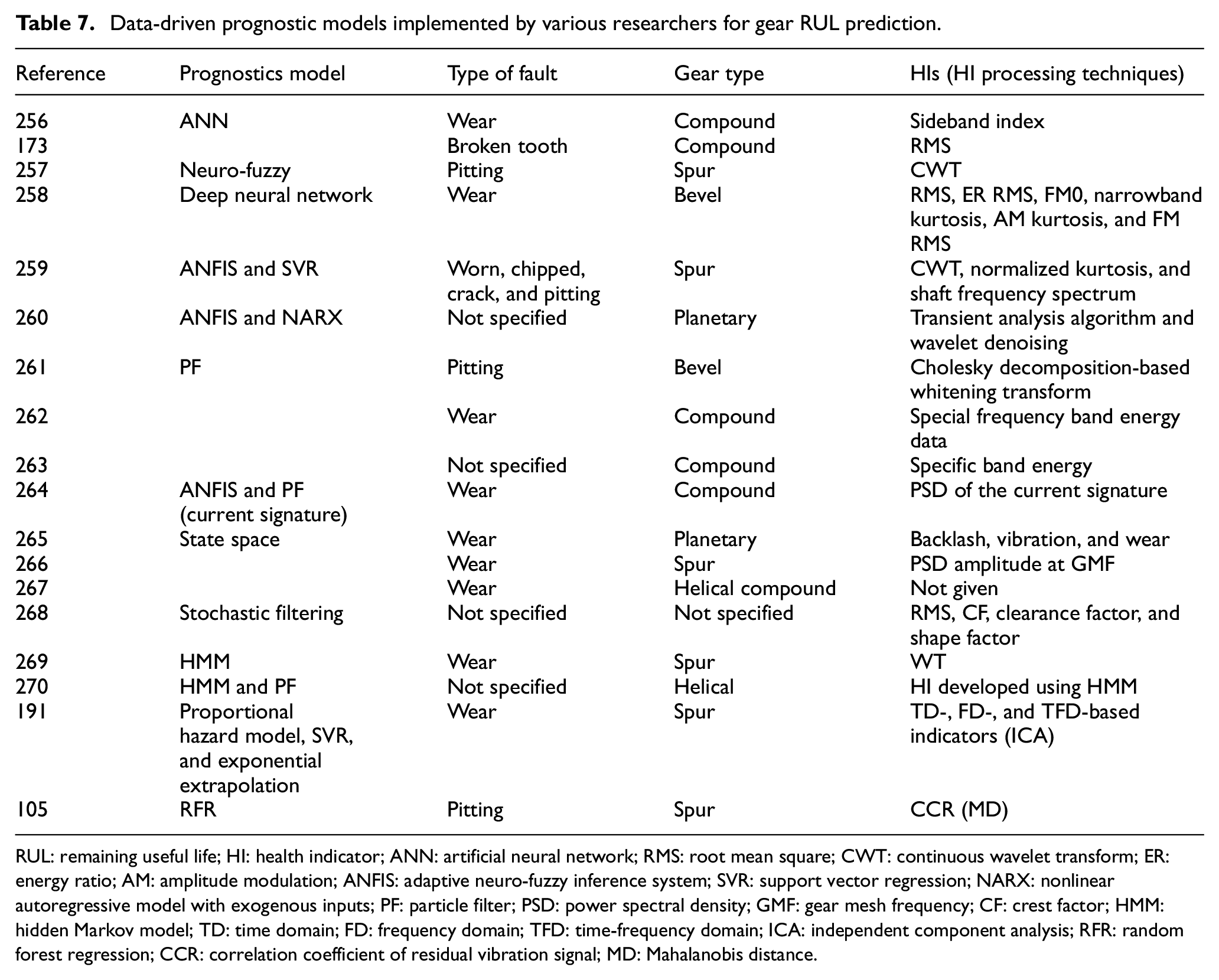
RUL: remaining useful life; HI: health indicator; ANN: artificial neural network; RMS: root mean square; CWT: continuous wavelet transform; ER: energy ratio; AM: amplitude modulation; ANFIS: adaptive neuro-fuzzy inference system; SVR: support vector regression; NARX: nonlinear autoregressive model with exogenous inputs; PF: particle filter; PSD: power spectral density; GMF: gear mesh frequency; CF: crest factor; HMM: hidden Markov model; TD: time domain; FD: frequency domain; TFD: time-frequency domain; ICA: independent component analysis; RFR: random forest regression; CCR: correlation coefficient of residual vibration signal; MD: Mahalanobis distance.

Neural network

The architecture of the ANN model discussed in section “Neural network” for gear fault classification is the same for fault prognosis with the exception of the target variable. The state of the gear fault in the form of 1, 0, −1, and so on was output in the ANN classification model, whereas the output variable in the prognostic model is the RUL. In all the reported work for the gear RUL prediction based on the ANN model, a nonlinear mapping between the subset of the past HI values and future HI values is considered. For RUL prediction, all these models extrapolate the HI value based on the past HI values. Zhang et al.²⁵⁶ used a back propagation ANN model for estimating the degradation trend of the sideband-based HI developed for a gear subjected to wear failure mode. The ANN model is combined with the change point detection method and the window adjusting method for enhancing the RUL prediction capability of the model. The recurrent neural network (RNN) model can better process and extrapolate the time series compared to the feed-forward neural network.²⁷¹ Hence, Tian and Zuo¹⁷³ used RNN for multi-step-ahead prediction of RMS-based HI for gear RUL prediction. In this work, the RMS indicator was fitted with the Weibull hazard rate in order to reduce the fluctuation in the HI value and hence improve the accuracy of the RUL prediction.

For further improvement in the accuracy of the neural network model, the ANN model is combined with some other artificial intelligence (AI)-based model. For example, Wang et al.²⁵⁷ used a neuro-fuzzy (NF) network to estimate the RUL one step ahead. Significant accuracy in prediction was observed with the NF network compared to the RNN model when trained with a large amount of training data. Deutsch and He²⁵⁸ used a deep belief feed-forward NN algorithm for RUL prediction of the bevel gear subjected to pitting. Six HIs, namely, residual RMS, energy operator RMS, FM0, narrowband kurtosis, AM kurtosis, and FM RMS were extracted from the raw vibration signal and used as inputs to the neural network for gear RUL prediction. The advantage of the DNN model over the conventional ANN is that it reduces the manual processing and analysis of the data by human experts. These methods are therefore suitable for automatic data processing and HI extraction for big data.

Particle filter

The PF is a Monte-Carlo approximation method that can monitor dynamic systems. The PF-based approach first creates the analytical/mathematical model that describes the component degradation process, and later, this degradation model is used to predict the future evolution of the component state and hence predict the RUL. Based on the past and present values of the available degradation data, the PF approach is used to calibrate the model parameters by assuming a probabilistic measurement model that links the measurement data with the component degradation.²⁷² He et al.²⁶¹ and Jia et al.²⁶² used the PF algorithm for predicting the RUL for a gear subjected to pitting and wear, respectively.

The PF approach can’t be directly implemented if the current state of the gear is not available.²⁷² Hence, some researchers integrated the PF model with some AI-based approaches; the later can be used for estimating the current state of the gear. For example, Cheng et al.²⁶⁴ combined the adaptive neuro-fuzzy inference system (ANFIS) and PF algorithm for RUL prediction of a wind turbine gear subjected to wear failure mode. Based on the learned state transition function from ANFIS, the RUL was predicted using the PF algorithm.

If multiple observation indicators/sensors such as vibration, noise, and acoustics are used for the RUL prediction, then the conventional PF cannot be used as it deals with a single observation indicator. Hence, Ni et al.²⁶⁵ used an adaptive state-space model for the RUL estimation of a planetary gear. Using different types of sensor data such as wear, vibration, and backlash, three RUL prediction models were developed: (a) considering the wear and backlash data, (b) considering the wear and vibration data, and (c) considering wear, backlash, and vibration data. The highest accuracy was observed with the third model, as this model was developed using the data from three different kinds of sources.

Working on similar lines to the PF algorithm, other nonlinear state-space models have also proposed for the gear RUL prediction in the past.^{266–270,273}

Miscellaneous

Most of the approaches for gear prognosis in the literature are either state space-based or ANN-based. A few other possible prognostic models were tried for gear RUL prediction. Roulias¹⁹¹ compared the performance of three RUL prediction models: (1) proportional hazards model, (2) ε-support vector regression (ε-SVR), and (3) exponential extrapolation based on bootstrap sampling. The TD-, FD-, and wavelet packet (WP) energy-based HIs extracted from AE and vibration data were fused using ICA. The ε-SVR was highlighted as the highly efficient method for gear fault prognosis if sufficient training data was available. It was observed that the exponential extrapolation method works best for the gear RUL prediction in the absence of sufficient training data. Samanta and Nataraj²⁵⁹ compared the performance of two AI-based techniques, that is, SVR and ANFIS, for extrapolating the trend of different HIs developed for different kinds of gear faults, that is, worn, chipped, cracked, and pitting. The performance of the SVR model was found better than the ANFIS model. Hussain and Gabbar²⁶⁰ compared the performance of the ANFIS model with the nonlinear autoregressive model with exogenous inputs (NARX) model for predicting the trend of the HI developed for planetary gearbox health monitoring. Comparable prediction performance from both algorithms was observed. However, the performance of the NARX model was observed slightly higher than the ANFIS model.

The data-driven prognostic models such as ANN and PF have been extensively studied while the random forest regression (RFR), one of the better-known algorithms for performing regression tasks, is relatively unexplored in the area of gear fault prognosis. The RFR methodology builds multiple weak and diverse decision trees and ensembles them together to get a more accurate and stable RUL prediction.²⁷⁴ Kundu et al.¹⁰⁵ presented the RFR approach for RUL prediction of a spur gear subjected to natural pitting progression. HIs such as CCR, RMS, peak, CF, M6A, FM4, NA4, and ER were used as inputs to the prognostic model. As mentioned earlier, the RFR approach has an inbuilt best HI selection capability, and using this model, the CCR was found to be the best HI for estimating the RUL. Based on the best HI (CCR), the RUL of the gear was predicted. In addition, the fusion of the CCR indicators extracted from the vibration sensor signals drawn from different sensor locations using the MD approach has been shown to be more effective in the RUL prediction compared to the RUL prediction using a single sensor-based CCR indicator. Elforjani²⁷⁵ proposed a combined diagnostic and prognostic model for health monitoring of a wind turbine gearbox. The RUL was predicted using four different models such as ANN, decision tree, SVM, and Gaussian process. The highest prediction accuracy was obtained with the Gaussian process model and the lowest accuracy with the ANN model.

Hybrid approaches

It is well known that data-driven prognostic models give better accuracy provided a large amount of training data is available. Such a kind of extensive data may not be readily available in practice. In addition, this approach is time-consuming as one has to wait for the failure to happen while the data from the sensors are collected over a long period of time. In addition, if one wishes to develop a data-driven model based on lab-scale test data instead of the field failure data (that may take a longer time), the cost of performing the experiments is high. Hence, for prognostics, a physics-based degradation model that gives a close and accurate relationship between the extent of the damage on the gear tooth and time can be a preferred alternative. However, the accuracy of the prediction by a physics-based prognostic model depends on how accurate the model captures the physics of the system and the exact role of multiple variables that influence the damage progression. Even if the model is built with reasonable accuracy, the prediction is influenced by the current stage fault diagnosis information (exact information of the type of failure mode and its severity). It is difficult to assess the current physical health condition of the component without interrupting the machine operation. Researchers have developed the dynamic models discussed in section “Dynamic models” to simulate response due to such kind of failure mode in gear. However, these simulation models are not validated with the actual field data. In addition, the physics-based diagnostic models may also give a high error in prediction if the parameters used in the model do not represent the physical system accurately. Data-based models discussed in section “Gear fault diagnostics” are very good in diagnosis compared to the physics-based diagnostic model. Hence, the physics-based prognostic models assume that the current health condition could be estimated from the sensor data.¹⁶

The hybrid prognostic model exploits the benefits of both physics and data-driven models. They are expected to give a better prediction, effectively harnessing the diagnosis accuracy benefits of the data-driven approaches and prognosis accuracy benefits of the physics-based approaches. Figure 6 shows a possible architecture for a hybrid framework for fault diagnostics and prognostics. A very few works dealing with the hybrid prognostic model for gear are reported and are mainly restricted to a tooth crack failure mode only.

Figure 6.

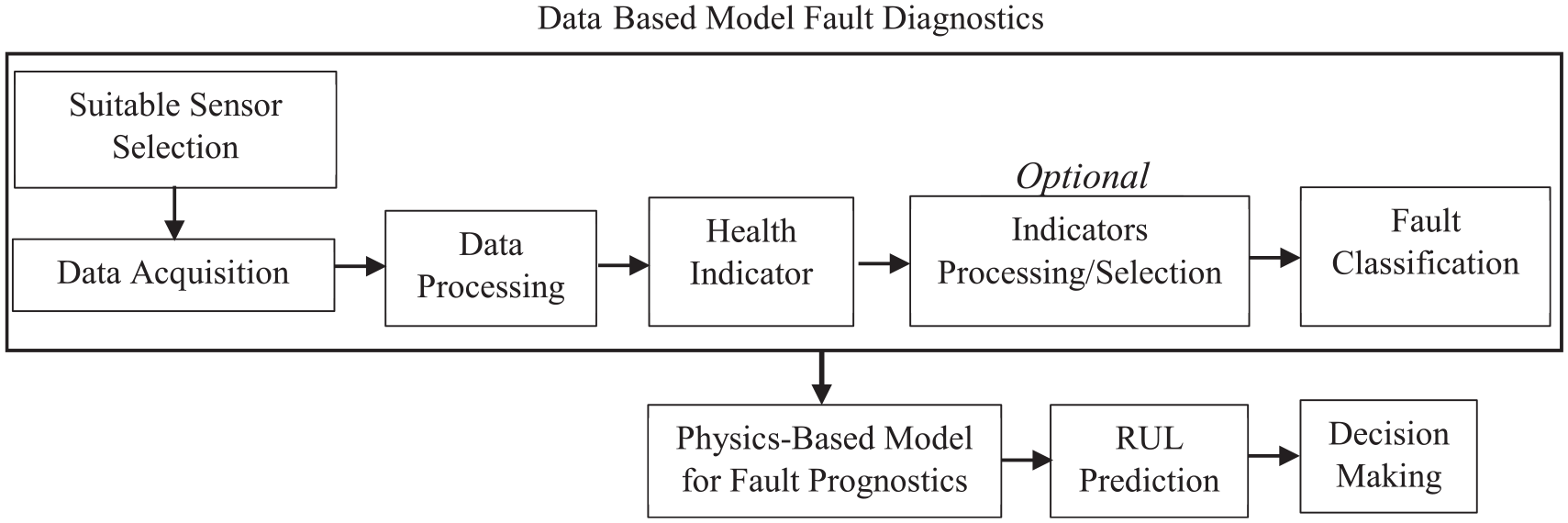
A hybrid framework for fault diagnostics and prognostics.

Zhao et al.²⁷⁶ proposed a hybrid model for estimating the gear life subjected to the gear tooth crack failure mode. The hybrid model in this work is divided into several parts: a gear FE model for gear stress analysis, a gear dynamic model for dynamic load calculation, and then a Paris power law equation for RUL estimation as was proposed by Li and Choi⁴⁵ and Li and Lee⁴⁷ discussed in section “Crack.” Using the HI extracted from the CM data, the current crack length on the gear tooth was predicted. Based on predicted crack length, the fatigue model parameters were updated using the Bayesian inference and RUL was estimated. Uncertainty and error in prediction was found to decrease with the availability of more crack length data and corresponding updating of Paris power law equation model parameters using Bayesian inference. In this study, simulated degradation data is used to show the effectiveness of the proposed methodology. Later, the same work is extended by Zhao et al.,²⁷⁷ in which a polynomial chaos expansion approach was used to evaluate the uncertainty in RUL prediction and likelihood function of Bayesian inference. The same work was further extended by Zhao et al.,²⁷⁸ in which a hybrid prognostics model was developed for gear under time-varying operating conditions. In practical cases, a sudden shock on the gear tooth surface may suddenly increase the damage size and creates a jump in the degradation path that reduces the gear life. In a further extension of the work proposed in Zhao et al.,²⁷⁶ Zhao et al.²⁷⁹ address this problem by proposing a hybrid prognostics model which considers the uncertainty of crack initiation time and random shock.

Similar to the above-mentioned studies, Kacprzynski et al.²⁸⁰ proposed a hybrid prognostics model for a spiral bevel pinion gear of a helicopter gearbox under gear tooth crack failure mode. Based on the fusion of some of the vibration-based indicators, gear crack severity level was predicted and then using physics-based model, propagation of crack size till a threshold crack length was estimated. Choi and Li²⁸¹ also proposed the hybrid prognostics model for a spur gear subjected to tooth crack failure mode. The feed-forward neural network model was used for estimating the crack size. The ANN model predicts the crack length based on HIs extracted using the raw vibration data. Based on the estimated crack length, the future evolution of the crack length was predicted for RUL prediction using the Paris power law equation. Zhao et al.⁷⁹ proposed a hybrid prognostic model for a spur gear subjected to surface wear failure mode. Based on the metal particle data, the mass loss from the gear tooth surface was estimated. Based on this estimated mass loss in the current state of the gear, the Archard’s wear model was used for predicting the future evolution of the wear on the gear tooth surface. The Bayesian inference approach was used to reduce the uncertainty and error in RUL prediction and to update the wear coefficient parameter in the Archard’s wear model. The posterior distribution of the wear coefficient parameter was found to become narrower and uncertainty and error in the RUL prediction is found to reduce with more availability of the mass loss data.

Basically, all the hybrid models for gear integrate material-level fatigue models, system-level data fusion algorithms, or data-based diagnostic and model parameter tuning techniques for the RUL prediction.

In general, due to a lack of insights/understanding of complex real-life conditions, it is often easy and convenient to neglect/overlook certain practical considerations while developing models in a laboratory environment.¹⁶ For the implementation of the PHM framework, for an industry environment, some PHM standards given by a different organization or researchers^282–286 can be referred. In addition, the 5S (streamline, smart processing, synchronize and see, standardize, and sustain) approach given by Lee et al.⁹ for systematic PHM design and implementation may also be referred.

Uncertainty quantification of prognostic approaches

The prognostic approaches should not only predict the RUL but also report the associated uncertainty of prediction or probability.²⁸⁷ The single point estimation of RUL is usually considered meaningless in industries. Hence, the decision making can be more convenient when the predicted RUL is reported with the associated uncertainty of the prediction. The importance of the uncertainty quantification during prognostics modeling is highlighted in Engel et al.²⁸⁸ and Saha and Goebel.²⁸⁹ Zhao et al.²⁷⁶ summarized the different sources of uncertainty and various uncertainty quantification activities. Shrestha and Solomatine²⁹⁰ gives an overview of uncertainty quantification for different approaches such as linear regression, nonlinear regression, decision tree, locally weighted regression, and fuzzy c-means clustering. In general, the uncertainty is expressed in the form of upper and lower quantiles of the underlying distribution of prediction errors.²⁹⁰ Figure 7 shows an example of the representation of uncertainty in RUL prediction. The upper and lower RUL prediction interval quantifies the model uncertainty and a narrower prediction interval width implies a lower model uncertainty. In the initial stage of gear life, the gear fault propagation-related information is less informative and loading conditions need to be assumed for a longer period of time. Hence, in the initial stage of gear life, RUL is predicted with a large amount of uncertainty. Whereas near to end of the gear life, the loading conditions need to be assumed for a shorter period of time and therefore uncertainty in prediction is less. In general, the uncertainty in prediction decreases with time.²⁷⁶

Figure 7.

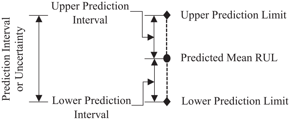
An example of uncertainty in RUL prediction.

The prognostic approaches estimate the RUL in the form of a PDF based on which model uncertainty is estimated. Using the central limit theorem, based on RUL prediction distribution mean and standard deviation parameters, the uncertainty in RUL prediction can be obtained¹⁰⁵

RU L_{upper, lower} = μ_{RUL} \pm Z_{α / 2} \frac{σ}{\sqrt{n}}

(14)

where $RU L_{upper, lower}$ represents the upper RUL and lower RUL values around the mean $μ_{RUL}$ , $Z_{α / 2}$ is the standard normal variate corresponding to the α-confidence interval, $n$ is the total number of samples used for estimating the RUL distribution, and $σ$ is the RUL distribution standard deviation parameter value.

Different methods have been used for quantifying the uncertainty in RUL prediction. According to Shrestha and Solomatine,²⁹⁰ the uncertainty of the prognostics model can be estimated using four ways:

Probabilistic-based methods: In the probabilistic-based methods, the model parameters are associated with uncertainty with some distribution parameters. The random samples of parameters are drawn from the distribution and based on which predictive distribution for model output, that is, RUL is obtained.^91,227,291 In the probabilistic-based methods, the Bayesian approach is the most widely used for interpreting the uncertainty in RUL prediction, especially in physics-based prognostic approaches.

Model error-based methods: In these methods, the model uncertainty is estimated through statistical properties of the error while producing the observed data.²⁹⁰ Many of the machine learning and statistical models used this method for prediction uncertainty estimation. The studies reported in previous studies^292–294 can be referred for a detailed study on these methods.

Resampling methods: The ensemble learning-based methods belong to this category. The RFR is the most widely method used in this category for estimation of the prediction uncertainty. In the resampling methods, out of the total available data set, “b,” random samples are bootstrapped/resampled each time to train a model. This process is repeated “B,” times and hence “B,” number of predictions are available for uncertainty quantification. The studies reported in Kundu et al.¹⁰⁵ and Kasiviswanathan et al.²²⁷ can be referred for resampling-based methods for uncertainty quantification.

Fuzzy-based: In the fuzzy-based methods, the model inputs and parameters are represented as a fuzzy number for defining the variability and to quantify the prediction uncertainty.²²⁷ The studies reported in Shrestha and Solomatine²⁹⁰ and Maskey et al.²⁹⁵ can be referred for fuzzy-based methods for uncertainty quantification.

Some prognostic approaches have inbuilt uncertainty quantification capability, whereas some approaches are integrated with uncertainty methods discussed above for quantification of uncertainty in predicted RUL. For example, Kundu et al.¹⁰⁵ used an ensemble decision tree-based RFR methodology for RUL prediction with associated uncertainty. The RFR methodology has an inbuilt uncertainty quantification capability. As discussed earlier, the RFR approach constructs $n$ number of decision trees for RUL prediction. Each individual decision tree gives different prediction of RUL. The mean and standard deviation obtained using the prediction from individual decision trees was used for quantifying the uncertainty of RUL prediction. The neural network-based models are working as a black-box. Hence, it is difficult to interpret the prediction and gauge the reliability of the predictions using neural network-based models.²⁹⁶ Few researchers overcome this issue by combining neural network-based approaches with uncertainty methods. For example, Kasiviswanathan et al.²²⁷ applied uncertainty methods such as bootstrap and Bayesian in ANN. The resampling method discussed above is used for uncertainty estimation using bootstrap methods. In the Bayesian neural network method, the weights are characterized by statistical distributions rather than constant values in a simple neural network. Vishnu et al.²⁹⁶ used the ensemble of long short-term memory (LSTM)-based deep learning networks integrated with deep ordinal regression models to estimate the uncertainty in RUL prediction. Similarly, Liu et al.²⁸⁷ integrate the LSTM approach with the Gaussian process regression model for estimating the uncertainty in RUL prediction. Trinchero et al. integrate the SVM model with the polynomial chaos approach for uncertainty quantification in the prediction made by the SVM approach. The above reported work highlighted the uncertainty quantification in data-driven prognostic approaches. The uncertainty quantification in physics-based prognostic approaches is mostly based on the Bayesian approach. One of the examples of the Bayesian approach for interpreting the RUL prediction uncertainty is discussed in section “Parameters updating of the physics-based prognostic models.” In addition, uncertainty quantification in the physics-based crack and wear growth prognostic problem is also discussed in section “Hybrid approaches.”

Performance evaluation metrics

The performance metrics are used to quantify the uncertainty and error of the prognostic/classification algorithms. The performance metrics allow the user to compare different models, understand the validity of a prognostic/classification estimation, and model performance characterization over different operating regimes.^297,298 The metrics for fault classification and fault prognosis are completely different due to the difference in the output of the two processes.

Metrics for evaluating the performance of the fault classification approaches

The confusion matrix is usually created for checking the correctness and accuracy of a classifier model. The confusion matrix is a table with its size based on the number of classes in both dimensions. Table 8 shows how a confusion matrix can look like for a two-class problem. In Table 8, the true positives (TP), false negatives (FN), false positives (FP), and true negatives (TN) stand for the number of instances the model predicts a healthy class as healthy, a healthy class as faulty, a faulty class as healthy, and a faulty class as faulty, respectively. The FP are also termed as a Type-I error and the FN are termed as Type-II error. The confusion matrix itself is not a performance measure as such. Still, most of the performance metrics for a classifier model are based on the confusion matrix and its values.

Table 8.

A confusion matrix.

		Predicted
		Healthy	Faulty
Actual	Healthy	True positives	False negatives
	Faulty	False positives	True negatives

Some of the performance metrics commonly used are as follows:

TP Rate: It is the rate at which the classification model correctly classifies the healthy class into a healthy class. It is the ratio of TP to the sum of TP and FN. It is also called sensitivity, recall, or hit rate.

TN Rate: It is the rate at which the classification model correctly classifies the faulty class into a faulty class. It is the ratio of TN to the sum of TN and FP. It is also called specificity or selectivity.

FN Rate: It is the rate at which the classification model incorrectly classifies the healthy class into a faulty class. It is the ratio of FN to the sum of TP and FN.

FP Rate: It is the rate at which the classification model incorrectly classifies the faulty class in a healthy class. It is the ratio of FP to the sum of TN and FP.

Metrics for evaluating the performance of the fault prognosis approaches

Performance metrics for prognostics should quantify factors like sensitivity to small changes, resistance to outliers, and usefulness for decision making. There is no single metric that can capture all these factors. The four major parameters such as uncertainty with some confidence bound, accuracy, precision, and timeliness are used for checking the RUL prediction model performance. The prognosis output should have two components: RUL or an estimated time to failure (ETTF) and the associated uncertainty. As discussed earlier in section “Uncertainty quantification of prognostic approaches,” subsequent to knowing the RUL value, the decision-making activity is more adaptive and effective if the RUL value is provided with the associated uncertainty rather than only a single predicted value.¹¹ Without uncertainty estimation, the prediction loses its significance.¹⁰⁵ The accuracy measures the closeness of the actual value to the predicted value. The precision measures the narrowness of the interval in which RUL falls and checks how close the predictions are clustered together. For every model, high accuracy and precision are required, but the same level of accuracy and precision in RUL is difficult to obtain in all the models. Hence, model selection is a key parameter for accurate RUL prediction. Timeliness measures the relative position of the PDF of the predicted model along the time axis.

The most widely used prognosis performance metrics in literature are mean square error (MSE)^{180,228,299,300} and mean absolute percentage error (MAPE).¹⁹⁰ However, these metrics are scale-dependent. The other performance metrics proposed include prognostics horizon, relative accuracy, convergence, α-λ performance, and so on. The development of performance metrics for a prognostic model is discussed in Saxena and colleagues.^297,301

Post prognostics decision making/health management process

Most of the gear failures take time to grow and reach a threshold of failure. In that scenario, using the RUL prediction results, the decision-making process provides the economic benefits, by exploiting the gear service life, adjusting the gear maintenance cycles, improving safety by adjusting the operating conditions, and so on, reduces life cycle costs, and reduces catastrophic failures.^6,302 In addition, the decision making step may also involve optimum allocation of resources/inventory, managing the logistic chain, an extension of production, and so on.³⁰³ The utilization of prognostic results in the decision-making process has not matured as yet. The decision-making strategies specific to gear health management is not available in the literature. However, in general, a few strategies are presented in the literature to optimize the maintenance activities based on the predicted RUL. For example, based on the predicted RUL, Lei and Sandborn³⁰⁴ proposed a real options analysis approach to determine the optimum predictive maintenance opportunity for a subsystem in a wind turbine. Skima et al.³⁰² addressed the post prognostics decision-making process for a micro-electro-mechanical system (MEMS). In this work, the decision-making problem is solved for distributed MEMS systems in which a set of autonomous equipment communicate and interact with each other to achieve a common mission. Camci et al.³⁰⁵ integrate the PHM information into maintenance and logistic infrastructure in order to reduce development, production, and ownership costs for the next-generation fighter aircraft. In the absence of precise RUL information, industries usually suffered from production loss and material wastage due to unplanned failure of the machine in the middle of the operation. To overcome this, Asmai et al.³⁰⁶ designed a framework for production scheduling based on the predicted RUL.

Based on multiple case studies conducted in different industries, Tiddens et al.³⁰⁷ presented a generalized framework to implement prognostics technologies for maintenance decision making. Chebel-Morello et al.³⁰³ presented many concepts of decision making based on expert knowledge of the system and predicted RUL. Based on the RUL prediction results, an example of reducing the predictive maintenance-related costs via appropriate planning is also discussed in this work. A bibliographic overview of different decision-making approaches is given in this work. Hence, for a detailed study on post prognostics decision-making process, this work may be referred. Based on the above discussion, for mechanical components such as gear, the decision-making process can be broadly divided into two categories: maintenance optimization and mission reconfiguration. For a detailed study, previous works^308–311 may be referred for the former category, whereas the work by Asmai et al.³⁰⁶ may be referred for the latter category.

Concluding remarks

The present work reviews different diagnostic and prognostic approaches, which encompass major activities of the PHM related to gears. A wide variety of sensors and its associated data processing approaches have been explored in developing diagnostic and prognostic approaches in the geared system. However, this review has, in particular, focused on the vibration sensor-based approaches.

Substantial investigations have been undertaken in major aspects of the fault identification, fault modeling, and fault propagation models of different fault categories in gears. Based on the literature reviewed, challenges and future directions in different aspects of the gear diagnostics and prognostics are enlisted as follows:

1. Fault diagnostics

• Hybrid faults

Researchers have investigated the dynamic response and developed physics-based and data-driven diagnostics and prognostics model for individual failure modes such as pitting, crack, and wear separately. These studies can be further extended for investigating the hybrid faults on the gear tooth surface. Since the combination of failure modes may sometimes appear in a practical situation, the complexity of the model can be very challenging in such scenarios.

HI development

A very few HIs exist that are sensitive for the entire range of gear life cycle. Some indicators are sensitive in the early stage of the gear fault, while others are sensitive in the advanced stage of the gear fault. Similarly, since most of the studies are based on the discrete amount of seeded gear fault size, it is still not clear which way many of these proposed indicators would behave during the gradual changes in the different health stages of the gear or during a complete life cycle for a particular kind of failure mode. Some of the recent signal processing approaches obliviate the need of a reference signal and the corresponding sensor (as required in many of the TSA-based techniques) during development of these HIs.

Definition of health stage division

Most of the gear failure modes are progressive in nature. With the development of a particular fault size, the trend of HI value varies. The degradation process of the gear can be divided into various stages based on the change in the value of physical damage or HI. Different quantification criterion is considered by various researchers to define the health stage division. However, no standard method is available in the literature to establish the division of these health stages for the gear.

2. Fault prognostics

Mainly due to the non-availability of enough run to failure test data for the gears, fewer studies exist for data-driven gear fault prognostics in contrast to the many for bearing, battery, and so on. Although there are many fault diagnostic approaches developed for gears, extensive studies on prognostic approaches, particularly with different operating parameters, may be pursued to increase confidence in the proposed prognostic approaches. The future prognostic approaches may involve further work on the stochastic nature of the lubrication, surface quality, hardening/heat treatment, and so on.

Change in operating condition

The data-driven prognostics and fault severity classification models are designed for particular operating conditions. Hence, if the operating conditions change for a system, then the historical data for that particular value of operating conditions is required. This leads to developing new prognostic and classifier models, which is costly both in terms of time and extensive experimentation. However, recently deep transfer learning-based classifier models are being developed. Such models use data obtained from one operating condition as a historical dataset for model training and predict fault severity level/types for other operating condition datasets. Similarly, the transfer learning-based developed models for gear fault severity/types classification can be used to develop a transfer learning-based gear RUL prediction model.

Prediction of the RUL in the field based on data obtained from the laboratory environment

Most of the data-driven prognostic models for gears have been developed based on the data obtained from specific test rigs at research laboratories. In most of the field applications, run-to-failure data may not be available to develop the prognostics model for a different size/capacity of the field gearbox vis-à-vis laboratory test setup. In such scenarios, the approaches to extrapolate the knowledge base on the prognostics model from research laboratories to the field application should be developed and explored for its accuracy, repeatability, and practicality. In literature, deep transfer learning models are being demonstrated to classify the fault severity level in the field based on the model trained using the laboratory test data. The idea can be further explored to predict the RUL in the field, based on the lab test data.

3. Definition of failure threshold

The failure threshold is typically defined based on the limiting value of damage or HI. Based on the size of the physical damage, the failure threshold for most of the gear failure modes is defined subjectively, not quantitatively. Some ISO standards are available to determine the failure threshold based on the value of HIs such as RMS and peak. In many of the studies reported in the literature, it was found that these HIs may not exhibit good sensitivity to monitor the damage progression in gear. Suitable guidelines to define the failure threshold for other HIs as well as based on the damage area may be desirable.

4. Integration of different approaches for a composite prognostics framework

Future research may need to be more focused on the integrated development of a prognostics framework involving alternate types, harnessing the strengths of the individual approaches. For example, the data-driven fault prognostic and fault severity classification models heavily rely on historical failure data. For a newly installed gearbox, the historical failure data may not be available. In such scenarios, integration of the dynamic models used in a physics-based framework and data-driven fault prognostics/classification model can improve the overall performance of the PHM activities. The fault prognostics/classifier models trained on simulated vibration data (obtained from the physics-based framework) can be used to predict the RUL/fault severity level for newly installed gears. For further improvement in the prediction accuracy, the trained classifier and prognostic models can be updated with data available from the actual field.

Footnotes

Declaration of conflicting interests

The author(s) declared no potential conflicts of interest with respect to the research, authorship, and/or publication of this article.

Funding

The author(s) received no financial support for the research, authorship, and/or publication of this article.

ORCID iD

Pradeep Kundu

References

Davis

JR.

Gear materials, properties, and manufacture. Materials Park, OH: ASM International, 2005.

Astridge

DG.

Helicopter transmissions-design for safety and reliability. Proc IMechE, Part G: J Aerospace Engineering 1989; 203: 123–138.

Ribrant

Bertling

LM.

Survey of failures in wind power systems with focus on Swedish wind power plants during 1997-2005. IEEE Trans Energy Convers 2007; 22: 167–173.

Department for Transport Air Accidents Investigation Branch. Aircraft accident report 2/2011, https://assets.publishing.service.gov.uk/media/5422f86aed915d13710006cb/2-2011_G-REDL.pdf (2011, accessed 10 May 2018).

Yoon

, et al. Gearbox tooth cut fault diagnostics using acoustic emission and vibration sensors—a comparative study. Sensors 2014; 14: 1372–1393.

Pecht

Kang

Prognostics and health management of electronics: fundamentals, machine learning, and the internet of things. Chichester: John Wiley, 2018.

Aye

Thiart

CJH

. A review of slow speed bearing diagnostics and prognostics. Int J Eng Sci Technol 2014; 6: 726–739.

Zio

. Prognostics and health management of industrial equipment. In: Kadry

(ed.) Diagnostics and prognostics of engineering systems: methods and techniques. Hershey, PA: IGI Global, 2013, pp. 333–356.

Lee

Zhao

, et al. Prognostics and health management design for rotary machinery systems—reviews, methodology and applications. Mech Syst Signal Pr 2014; 42: 314–334.

10.

Jardine

AKS

Lin

Banjevic

A review on machinery diagnostics and prognostics implementing condition-based maintenance. Mech Syst Signal Pr 2006; 20: 1483–1510.

11.

Sikorska

Hodkiewicz

Prognostic modelling options for remaining useful life estimation by industry. Mech Syst Signal Pr 2011; 25: 1803–1836.

12.

Peng

Dong

Zuo

MJ.

Current status of machine prognostics in condition-based maintenance: a review. Int J Adv Manuf Technol 2010; 50: 297–313.

13.

Atamuradov

Medjaher

Dersin

, et al. Prognostics and health management for maintenance practitioners—review, implementation and tools evaluation. Int J Progn Heal Manag 2017; 8: 1–31.

14.

Liang

Zuo

Feng

Dynamic modeling of gearbox faults: a review. Mech Syst Signal Pr 2018; 98: 852–876.

15.

Cubillo

Perinpanayagam

Esperon-Miguez

A review of physics-based models in prognostics: application to gears and bearings of rotating machinery. Adv Mech Eng 2016; 8: 1–21.

16.

Heng

Zhang

Tan

ACC

, et al. Rotating machinery prognostics: state of the art, challenges and opportunities. Mech Syst Signal Pr 2009; 23: 724–739.

17.

Dragomir

Gouriveau

Dragomir

, et al. Review of prognostic problem in condition-based maintenance. In: 2009 European control conference, Budapest, 23–26 August 2009, pp. 1587–1592. New York: IEEE.

18.

Ahmadzadeh

Lundberg

Remaining useful life estimation: review. Int J Syst Assur Eng Manag 2014; 5: 461–474.

19.

Condition monitoring in engineering asset management. In: 12th Asia-Pacific vibration conference, Sapporo, Japan, 6–9 August 2007, pp. 1–16.

20.

Sharma

Parey

A review of gear fault diagnosis using various condition indicators. Procedia Eng 2016; 144: 253–263.

21.

Sait

Sharaf-Eldeen

. A review of gearbox condition monitoring based on vibration analysis techniques diagnostics and prognostics. In: Conference proceedings of the society for experimental mechanics series, 2011, pp. 307–324. DOI: 10.1007/978-1-4419-9428-8_25.

22.

Aherwar

An investigation on gearbox fault detection using vibration analysis techniques: a review. Aust J Mech Eng 2012; 10: 169–183.

23.

Večeř

Kreidl

Šmíd

Condition indicators for gearbox condition monitoring systems. Acta Polytech 2005; 45: 35–43.

24.

Lebold

Mcclintic

Campbell

, et al. Review of vibration analysis methods for gearbox diagnostics and prognostics. In: Proceedings of the 54th meeting of the society for machinery failure prevention technology, 2000, pp. 623–634. DOI: 10.1017/CBO9781107415324.004.

25.

Aherwar

Khalid

Vibration analysis techniques for gearbox diagnostic: a review. Int J Adv Eng Technol 2012; 3: 4–12.

26.

McCall

JL.

Systematic analysis of gear failures. Metals Park, OH: American Society for Metals, 1986.

27.

Moallem

Akbarzadeh

Ariaei

Prediction of micropitting life in spur gears operating under mixed-lubrication regime using load-sharing concept. Proc IMechE, Part J: J Engineering Tribology 2016; 230: 591–599.

28.

Institute

Gearbox: cracked or broken tooth, https://www.mobiusinstitute.com/site2/item.asp?LinkID=8061&iVibe=1&sTitle=Gearbox (2019, accessed 19 August 2019).

29.

Randall

RB.

A new method of modeling gear faults. Trans ASME J Mech Des 1982; 104: 259–267.

30.

McFadden

PD.

Detecting fatigue cracks in gears by amplitude and phase demodulation of the meshing vibration. J Vib Acoust Stress Reliab Des 1986; 108: 165–170.

31.

Rzeszucinski

Sinha

Edwards

, et al. Amplitude of probability density function (APDF) of vibration response as a robust tool for gearbox diagnosis. Strain 2012; 48: 510–516.

32.

Kundu

Darpe

Kulkarni

MS.

A correlation coefficient based vibration indicator for detecting natural pitting progression in spur gears. Mech Syst Signal Pr 2019; 129: 741–763.

33.

Kundu

Darpe

Kulkarni

MS.

Gear pitting severity level identification using binary segmentation methodology. Struct Control Heal Monit 2020; 27: e2478.

34.

Smith

Randall

, et al. Development of a gear vibration indicator and its application in gear wear monitoring. Mech Syst Signal Pr 2016; 76–77: 319–336.

35.

Pandya

Parey

Experimental investigation of spur gear tooth mesh stiffness in the presence of crack using photoelasticity technique. Eng Fail Anal 2013; 34: 488–500.

36.

Tian

Measurement of gear tooth dynamic deformation using dynamic speckle photography. Chinese Sci Bull 1998; 43: 514–518.

37.

Raghuwanshi

Parey

Experimental measurement of gear mesh stiffness of cracked spur gear by strain gauge technique. Measurement 2016; 86: 266–275.

38.

Åkerblom

Gear noise and vibration: a literature survey, http://www.diva-portal.org/smash/get/diva2:139878/FULLTEXT01.pdfinput (2001, accessed 19 August 2019).

39.

Paris

Erdogan

A critical analysis of crack propagation laws. J Fluids Eng Trans ASME 1963; 85: 528–533.

40.

Cai

Han

Hua

, et al. Study on stress intensity factors for crack on involute spur gear tooth. Adv Mech Eng 2015; 7: 1–12.

41.

Jelaska

Glodez

Kramberger

, et al. Numerical modelling of gear tooth root fatigue behaviour. In: Fatigue Crack Paths (FCP 2003), Parma, Italy, 18–20 September 2003.

42.

Aberšek

Flašker

Glodež

Review of mathematical and experimental models for determination of service life of gears. Eng Fract Mech 2004; 71: 439–453.

43.

Podrug

Glodež

Jelaska

Numerical modelling of crack growth in a gear tooth root. Stroj Vestnik/J Mech Eng 2011; 57: 579–586.

44.

Pehan

Hellen

Flasker

, et al. Numerical methods for determining stress intensity factors vs crack depth in gear tooth roots. Int J Fatigue 1997; 19: 677–685.

45.

Choi

Spur gear root fatigue crack prognosis via crack diagnosis and fracture mechanics. In: 56th Meet Soc Mech Fail Prev Technol, meeting of the society of mechanical failures prevention technology (MFPT), Virginia Beach, Virginia, 15–19 April 2002, pp. 311–320. Winchester, VA: Society for Machinery Failure Prevention Technology (MFPT).

46.

Karandikar

Kim

Schmitz

TL.

Prediction of remaining useful life for fatigue-damaged structures using Bayesian inference. Eng Fract Mech 2012; 96: 588–605.

47.

Lee

Gear fatigue crack prognosis using embedded model, gear dynamic model and fracture mechanics. Mech Syst Signal Pr 2005; 19: 836–846.

48.

Endeshaw

Ekwaro-Osire

Alemayehu

, et al. Evaluation of fatigue crack propagation of gears considering uncertainties in loading and material properties. Sustain 2017; 9: 2200.

49.

Glodež

Šraml

Kramberger

A computational model for determination of service life of gears. Int J Fatigue 2002; 24: 1013–1020.

50.

Chen

Jin

Liang

, et al. Propagation path and failure behavior analysis of cracked gears under different initial angles. Mech Syst Signal Pr 2018; 110: 90–109.

51.

Lin

Liu

Zhao

, et al. Fatigue life prediction of engaging spur gears using power density. Proc IMechE, Part C: J Mechanical Engineering Science 2018; 232: 4332–4341.

52.

Lewicki

Handschuh

Spievak

, et al. Consideration of moving tooth load in gear crack propagation predictions. J Mech Des Trans ASME 2001; 123: 118–124.

53.

Agarwal

Zagade

Khan

, et al. Fatigue crack propagation in a gear tooth in the presence of an inclusion. Int J Comput Methods Eng Sci Mech 2014; 15: 247–252.

54.

Gueye

Shao

Chen

Prediction of gear tooth crack propagation path based on pseudo evolutionary structural optimization. Int J COMADEM 2017: 20.

55.

Čular

Vučković

Žeželj

, et al. Analytical approach for low and high cycle bending fatigue life prediction of carburized gear steel specimens. Eng Fail Anal 2020; 108: 104328.

56.

Forman

Kearney

Engle

RM.

Numerical analysis of crack propagation in cyclic-loaded structures. J Basic Eng 1967; 89: 459–463.

57.

Mínguez

Foreman’s crack growth rate equation and the safety conditions of cracked structures. Eng Fract Mech 1994; 48: 663–672.

58.

Kacprzynski

Roemer

Modgil

, et al. Enhancement of physics-of-failure prognostic models with system level features. In: Proceedings, IEEE aerospace conference, Big Sky, MT, 9–16 March 2002, pp. 6-2919–6-2925. New York: IEEE.

59.

Pugno

Ciavarella

Cornetti

, et al. A generalized Paris’ law for fatigue crack growth. J Mech Phys Solids 2006; 54: 1333–1349.

60.

Ding

Rieger

NF.

Spalling formation mechanism for gears. Wear 2003; 254: 1307–1317.

61.

Yin

Chen

Y-X

Liu

Lifetime prediction for the subsurface crack propagation using three-dimensional dynamic FEA model. Mech Syst Signal Pr 2017; 87: 54–70.

62.

Fajdiga

Flašker

Glodež

, et al. Numerical modelling of micro-pitting of gear teeth flanks. Fatigue Fract Eng Mater Struct 2003; 26: 1135–1143.

63.

Rycerz

Olver

Kadiric

Propagation of surface initiated rolling contact fatigue cracks in bearing steel. Int J Fatigue 2017; 97: 29–38.

64.

Blake

Cheng

HS.

A surface pitting life model for spur gears: part I—life prediction. J Tribol 1991; 113: 712–718.

65.

Budynas

Nisbett

JK.

Shigley’s mechanical engineering design. 9th ed. New Delhi, India: Tata McGraw Hill Education Private Limited, 2015.

66.

Blake

Cheng

HS.

A surface pitting life model for spur gears: Part II-failure probability prediction. J Tribol 1991; 113: 719–724.

67.

Aslantaş

Taşgetiren

A study of spur gear pitting formation and life prediction. Wear 2004; 257: 1167–1175.

68.

Glodež

Ren

Flašker

Surface fatigue of gear teeth flanks. Comput Struct 1999; 73: 475–483.

69.

Zhu

Ren

Wang

QJ.

Pitting life prediction based on a 3D line contact mixed EHL analysis and subsurface von Mises stress calculation. J Tribol 2009; 131: 041501.

70.

Zaretsky

EV.

Fatigue criterion to system design, life, and reliability. J Propuls Power 1987; 3. DOI: 10.2514/3.22955.

71.

Kahraman

A micro-pitting model for spur gear contacts. Int J Fatigue 2014; 59: 224–233.

72.

Kahraman

Klein

A fatigue model for spur gear contacts operating under mixed elastohydrodynamic lubrication conditions. J Mech Des Trans ASME 2012; 134: 041007.

73.

Anisetti

A tribo-dynamic contact fatigue model for spur gear pairs. Int J Fatigue 2017; 98: 81–91.

74.

Billington

Zhang

, et al. Adaptive prognostics for rolling element bearing condition. Mech Syst Signal Pr 1999; 13: 103–113.

75.

Kurfess

Liang

SY.

Stochastic prognostics for rolling element bearings. Mech Syst Signal Pr 2000; 14: 747–762.

76.

Zhu

Martini

Wang

, et al. Simulation of sliding wear in mixed lubrication. J Tribol 2007; 129: 544–552.

77.

Archard

JF.

Contact and rubbing of flat surfaces. J Appl Phys 1953; 24: 981–988.

78.

Flodin

Andersson

Simulation of mild wear in spur gears. Wear 1997; 207: 16–23.

79.

Zhao

Tian

Liang

, et al. An integrated prognostics method for failure time prediction of gears subject to the surface wear failure mode. IEEE Trans Reliab 2018; 67: 316–327.

80.

Shifeng

Cheng

HS.

Sliding wear calculation in spur gears. J Tribol 1993; 115: 493–500.

81.

Cheng

HS.

A sliding wear model for partial-EHL contacts. J Tribol 1991; 113: 134–141.

82.

Bajpai

Kahraman

Anderson

NE.

A surface wear prediction methodology for parallel-axis gear pairs. J Tribol 2004; 126: 597–605.

83.

Liu

Zhu

, et al. Study on gear contact fatigue failure competition mechanism considering tooth wear evolution. Tribol Int 2020; 147: 106277.

84.

Hong

Wang

Tomovic

, et al. A novel indicator for mechanical failure and life prediction based on debris monitoring. IEEE Trans Reliab 2017; 66: 161–169.

85.

Ghosh

Paulson

Sadeghi

A fracture mechanics approach to simulate sub-surface initiated fretting wear. Int J Solids Struct 2015; 58: 335–352.

86.

Coppe

Pais

. Identification of equivalent damage growth parameters for general crack geometry. In: Annual conference of the prognostics and health management society, 2010, pp. 1–10, https://www.phmsociety.org/sites/phmsociety.org/files/phm_submission/2010/phmc_10_061.pdf

87.

Simani

Identification and fault diagnosis of a simulated model of an industrial gas turbine. IEEE T Ind Inform 2005; 1: 202–216.

88.

Peel

. Data driven prognostics using a Kalman filter ensemble of neural network models. In: 2008 international conference on prognostics and health management, Denver, CO, 6–9 October 2008, pp. 1–6. New York: IEEE.

89.

Orchard

Vachtsevanos

GJ.

A particle filtering approach for on-line failure prognosis in a planetary carrier plate. Int J Fuzzy Log Intell Syst 2007; 7: 221–227.

90.

Zio

Peloni

Particle filtering prognostic estimation of the remaining useful life of nonlinear components. Reliab Eng Syst Saf 2011; 96: 403–409.

91.

Choi

Kim

NH.

Prognostics 101: a tutorial for particle filter-based prognostics algorithm using Matlab. Reliab Eng Syst Saf 2013; 115: 161–169.

92.

Choi

Kim

A tutorial for model-based prognostics algorithms based on Matlab code. Ann Conf Progn Heal Manag Soc 2012; 2012: 1–9.

93.

Corbetta

Sbarufatti

Manes

, et al. Sequential Monte Carlo sampling for crack growth prediction providing for several uncertainties. In: Second European conference of the prognostics and health management society, 2014, pp. 1–13, https://core.ac.uk/download/pdf/55253841.pdf

94.

Oppenheimer

Loparo

Physically based diagnosis and prognosis of cracked rotor shafts. Aerosense 2002; 4733: 122–132.

95.

Saha

Goebel

Christophersen

Comparison of prognostic algorithms for estimating remaining useful life of batteries. Trans Inst Meas Control 2009; 31: 293–308.

96.

Zio

Baraldi

Cadini

, et al. Prognostics under different available information. Chem Eng Trans 2013; 33: 163–168.

97.

Jouin

Gouriveau

Hissel

, et al. Particle filter-based prognostics: review, discussion and perspectives. Mech Syst Signal Pr 2016; 72–73: 2–31.

98.

Kundu

Nath

Palani

, et al. Integrating GLL-Weibull distribution within a Bayesian framework for life prediction of shape memory alloy spring undergoing thermo-mechanical fatigue. J Mater Eng Perform 2018; 27: 3655–3666.

99.

Baraldi

Mangili

Zio

A Kalman filter-based ensemble approach with application to turbine creep prognostics. IEEE Trans Reliab 2012; 61: 966–977.

100.

Ray

Tangirala

Stochastic modeling of fatigue crack dynamics for on-line failure prognostics. IEEE Trans Control Syst Technol 1996; 4: 443–451.

101.

Simon

A comparison of filtering approaches for aircraft engine health estimation. Aerosp Sci Technol 2008; 12: 276–284.

102.

Wagner

Shoureshi

A robust failure diagnostic system for thermofluid processes. Automatica 1992; 28: 375–381.

103.

Laroche

Sedda

Durieu

Methodological insights for online estimation of induction motor parameters. IEEE Trans Control Syst Technol 2008; 16: 1021–1028.

104.

Al-arbi

Condition monitoring of gear systems using vibration analysis. University of Huddersfield, http://eprints.hud.ac.uk/17821/ (2012, accessed 9 August 2017).

105.

Kundu

Darpe

Kulkarni

MS.

An ensemble decision tree methodology for remaining useful life prediction of spur gears under natural pitting progression. Struct Heal Monit 2019; 19: 854–872.

106.

Sharma

Parey

Gear crack detection using modified TSA and proposed fault indicators for fluctuating speed conditions. Meas J Int Meas Confed 2016; 90: 560–575.

107.

Fan

Zhou

, et al. Gear tooth surface damage diagnosis based on analyzing the vibration signal of an individual gear tooth. Adv Mech Eng 2017; 9: 1–14.

108.

Combet

Gelman

An automated methodology for performing time synchronous averaging of a gearbox signal without speed sensor. Mech Syst Signal Pr 2007; 21: 2590–2606.

109.

Bechhoefer

Calculating a tachometer signal from onboard a smart vibration sensor. In: Proceedings of the annual conference of the prognostics and health management society PHM, 2018, https://www.phmpapers.org/index.php/phmconf/article/view/338

110.

Bonnardot

El Badaoui

Randall

, et al. Use of the acceleration signal of a gearbox in order to perform angular resampling (with limited speed fluctuation). Mech Syst Signal Pr 2005. doi:10.1016/j.ymssp. 2004.05.001

111.

Dempsey

PJ.

Integrating oil debris and vibration measurements for intelligent machine health monitoring. University of Toledo, https://ntrs.nasa.gov/archive/nasa/casi.ntrs.nasa.gov/20030056593.pdf (2003, accessed 9 August 2017).

112.

Randall

RB.

Vibration-based condition monitoring: industrial, aerospace and automotive applications. John Wiley & Sons, 2011. DOI: 10.1002/9780470977668.

113.

Mcclintic

Lebold

Maynard

, et al. Residual and difference feature analysis with transitional gearbox data. In: Proceedings of the 54th meeting of the society for machinery failure prevention technology, 2000. doi:10.1016/j.appet.2014.12.009

114.

Decker

Lewicki

DG.

Spiral bevel pinion crack detection in a helicopter gearbox. In: Proceeding 59th annual forum of the American helicopter society, Phoenix, AZ, 6–8 May 2003.

115.

Lei

Lin

, et al. A review on empirical mode decomposition in fault diagnosis of rotating machinery. Mech Syst Signal Pr 2013; 35: 108–126.

116.

Kundu

Chopra

Lad

BK.

Multiple failure behaviors identification and remaining useful life prediction of ball bearings. J Intell Manuf 2019; 30: 1795–1807.

117.

Decker

HJ.

Crack detection for aerospace quality spur gears, https://apps.dtic.mil/dtic/tr/fulltext/u2/a403008.pdf (2002, accessed 16 September 2018).

118.

Mathew

Stecki

Comparison of vibration and direct reading ferrographic techniques in application to high-speed gears operating under steady and varying load conditions. Lubr Eng 1987; 43: 646–653.

119.

Limmer

JD.

Model-based condition index for tracking gear wear and fatigue damage. Wear 2000; 241: 26–32.

120.

Zakrajsek

Townsend

Decker

HJ.

An analysis of gear fault detection methods as applied to pitting fatigue failure data. NASA Technical Memorandum 105950, Report No. 92-C–035, 1993.

121.

Zakrajsek

Handschuh

Lewicki

, et al. Detecting gear tooth fracture in a high contact ratio face gear mesh, 1995, https://ntrs.nasa.gov/archive/nasa/casi.ntrs.nasa.gov/19950012710.pdf (accessed 16 September 2018).

122.

Decker

Handschuh

Zakrajsek

. An enhancement to the NA4 gear vibration diagnostic parameter. NASA Technical Memorandum 106553, ARL-TR-389, 1994, 20 pp., https://ntrs.nasa.gov/archive/nasa/casi.ntrs.nasa.gov/19940033010.pdf

123.

Zakrajsek

Handschuh

Decker

HJ.

Application of fault detection techniques to spiral bevel gear fatigue data. NASA Technical Memorandum 106467, ARL-TR-345, 1994, 14 pp.

124.

Combet

Gelman

Novel adaptation of the demodulation technology for gear damage detection to variable amplitudes of mesh harmonics. Mech Syst Signal Pr 2011; 25: 839–845.

125.

Mark

Lee

Patrick

, et al. A simple frequency-domain algorithm for early detection of damaged gear teeth. Mech Syst Signal Pr 2010; 24: 2807–2823.

126.

Hines

Mark

WD.

Bending-fatigue damage-detection on notched-tooth spiral-bevel gears using the average-log-ratio, ALR, algorithm. Mech Syst Signal Pr 2014; 43: 44–56.

127.

Mark

Hines

JA.

Frequency-domain assessment of gear-tooth bending-fatigue damage-progression using the average-log-ratio, ALR, algorithm. Mech Syst Signal Pr 2014; 45: 479–487.

128.

Ziaran

Darula

Determination of the state of wear of high contact ratio gear sets by means of spectrum and cepstrum analysis. J Vib Acoust 2013; 135: 021008.

129.

Combet

Gelman

Optimal filtering of gear signals for early damage detection based on the spectral kurtosis. Mech Syst Signal Pr 2008; 23: 652–668.

130.

Barszcz

Randall

RB.

Application of spectral kurtosis for detection of a tooth crack in the planetary gear of a wind turbine. Mech Syst Signal Pr 2009; 23: 1352–1365.

131.

Polyshchuk

Choy

Braun

MJ.

Gear fault detection with time-frequency based parameter NP4. Int J Rotating Mach 2002; 8: 57–70.

132.

Polyshchuk

Choy

Braun

MJ.

New gear-fault-detection parameter by use of joint time-frequency distribution. J Propuls Power 2000; 16: 340–346.

133.

Zheng

Chen

Gear fault diagnosis based on continuous wavelet transform. Mech Syst Signal Pr 2002; 16: 447–457.

134.

Vernekar

Kumar

Gangadharan

KV.

Gear fault detection using vibration analysis and continuous wavelet transform. Procedia Mater Sci 2014; 5: 1846–1852.

135.

Deekshit

KKC

Chaitanya Kumar

Supraja

, et al. Comparison of DWT & WPT to detect bearing faults in 3 phase induction motor using current signature analysis. J Electr Eng 2015, http://www.jee.ro/covers/art.php?issue=WY1429270565W5530f02593afc

136.

Sun

, et al. Multiwavelet transform and its applications in mechanical fault diagnosis—a review. Mech Syst Signal Pr 2014; 43: 1–24.

137.

Chen

Pan

, et al. Wavelet transform based on inner product in fault diagnosis of rotating machinery: a review. Mech Syst Signal Pr 2016; 70–71: 1–35.

138.

Yan

Gao

Chen

Wavelets for fault diagnosis of rotary machines: a review with applications. Sig Process 2014; 96: 1–15.

139.

Meltzer

Dien

NP.

Fault diagnosis in gears operating under non-stationary rotational speed using polar wavelet amplitude maps. Mech Syst Signal Pr 2004; 18: 985–992.

140.

Zhu

Wang

, et al. Synchronous enhancement of periodic transients on polar diagram for machine fault diagnosis. Int J Wave Multiresol Inf Pr 2009; 7: 427–442.

141.

Rafiee

Tse

PW.

Use of autocorrelation of wavelet coefficients for fault diagnosis. Mech Syst Signal Pr 2009; 23: 1554–1572.

142.

Zuo

Lin

Fan

Feature separation using ICA for a one-dimensional time series and its application in fault detection. J Sound Vib 2005; 287: 614–624.

143.

Öztürk

Sabuncu

Yesilyurt

Early detection of pitting damage in gears using mean frequency of scalogram. J Vib Control 2008; 14: 469–484.

144.

Wang

Makis

Yang

A wavelet approach to fault diagnosis of a gearbox under varying load conditions. J Sound Vib 2010; 329: 1570–1585.

145.

Saravanan

Ramachandran

KI.

Incipient gear box fault diagnosis using discrete wavelet transform (DWT) for feature extraction and classification using artificial neural network (ANN). Expert Syst Appl 2010; 37: 4168–4181.

146.

Yan

Yuan

, et al. Virtual prototype and experimental research on gear multi-fault diagnosis using wavelet-autoregressive model and principal component analysis method. Mech Syst Signal Pr 2011; 25: 2589–2607.

147.

Parey

Tandon

Impact velocity modelling and signal processing of spur gear vibration for the estimation of defect size. Mech Syst Signal Pr 2007; 21: 234–243.

148.

Parey

El Badaoui

Guillet

, et al. Dynamic modelling of spur gear pair and application of empirical mode decomposition-based statistical analysis for early detection of localized tooth defect. J Sound Vib 2006; 294: 547–561.

149.

Zhao

Zhang

, et al. Gear crack level classification based on EMD and EDT. Math Probl Eng 2014; 2015: 1–10.

150.

Sharma

Parey

Frequency domain averaging based experimental evaluation of gear fault without tachometer for fluctuating speed conditions. Mech Syst Signal Pr 2017; 85: 278–295.

151.

Zhao

Yan

Gearbox fault diagnosis using complementary ensemble empirical mode decomposition and permutation entropy. Shock Vib 2016; 2016: 3891429.

152.

Sharma

Parey

Extraction of weak fault transients using variational mode decomposition for fault diagnosis of gearbox under varying speed. Eng Fail Anal 2020; 107: 104204.

153.

Xiao

A novel detrended fluctuation analysis method for gear fault diagnosis based on variational mode decomposition. Shock Vib 2018; 2018: 7045127.

154.

Xiao

Ding

, et al. Gear fault diagnosis based on kurtosis criterion VMD and SOM neural network. Appl Sci 2019; 9: 5424.

155.

Zhao

Huang

Qin

Fault diagnosis for gearbox based on improved empirical mode decomposition. Shock Vib 2015; 2015: 215806.

156.

Wang

McFadden

PD.

Early detection of gear failure by vibration analysis—I calculation of the time-frequency distribution. Mech Syst Signal Pr 1993; 7: 193–203.

157.

Wong

. Vibration-based helicopter gearbox health monitoring—an overview of the research program in DSTO. In: International Conference on Health and Usage Monitoring, 2001, pp. 1–12, http://www.humsconference.com.au/Papers2001/5-14.pdf

158.

Samuel

Pines

DJ.

A review of vibration-based techniques for helicopter transmission diagnostics. J Sound Vib 2005; 282: 475–508.

159.

Stewart

. Some useful data analysis techniques for gearbox diagnostics. Mach Heal Monit Group, Inst Sound Vib Res Univ Southampton, MHM/R/10/7, 1977.

160.

Swansson

. Application of vibration signal analysis techniques to condition monitoring. In: Lubrication friction and wearing in engineering, Melbourne, Australia, 1980, pp. 262–267. Barton, ACT, Australia: Institution of Engineers.

161.

Wang

Early detection of gear tooth cracking using the resonance demodulation technique. Mech Syst Signal Pr 2001; 15: 887–903.

162.

Wang

Xiang

Markert

, et al. Spectral kurtosis for fault detection, diagnosis and prognostics of rotating machines: a review with applications. Mech Syst Signal Pr 2016; 66–67: 679–698.

163.

Safizadeh

Lakis

Thomas

Using short-time Fourier transform in machinery diagnosis. In: 4th WSEAS international conference on electronic signal processing and control, 25–27 April 2005, pp.1–7. Stevens Point, Wisconsin: World Scientific and Engineering Academy and Society (WSEAS).

164.

Hong

Y-S

Ahn

S-H

Song

C-K

, et al. Component-level fault diagnostics of a bevel gear using a wavelet packet transform. Proc IMechE, Part E: J Process Mechanical Engineering 2011; 225: 1–12.

165.

Zhang

Brownjohn

Frequency modulated empirical mode decomposition method for the identification of instantaneous modal parameters of aeroelastic systems. J Wind Eng Ind Aerodyn 2012; 101: 43–52.

166.

Zhang

Peng

Chen

, et al. A gearbox fault diagnosis method based on frequency-modulated empirical mode decomposition and support vector machine. Proc IMechE, Part C: J Mechanical Engineering Science 2018; 232: 369–380.

167.

Liu

Guo

Tang

, et al. Multi-sensor data fusion using a relevance vector machine based on an ant colony for gearbox fault detection. Sensors 2015; 15: 21857–21875.

168.

Dang

A fault diagnosis scheme for rolling bearing based on particle swarm optimization in variational mode decomposition. Shock Vib 2016; 2016: 9372691.

169.

Zhang

Miao

Zhang

, et al. A parameter-adaptive VMD method based on grasshopper optimization algorithm to analyze vibration signals from rotating machinery. Mech Syst Signal Pr 2018; 108: 58–72.

170.

Zhou

Qiu

Dynamic strategy based parallel ant colony optimization on GPUs for TSPs. Sci China Inf Sci 2017; 60: 068102.

171.

Shen

Guo

, et al. Forecasting stock indices using radial basis function neural networks optimized by artificial fish swarm algorithm. Knowledge-based Syst 2011; 24: 378–385.

172.

Feng

Liang

Chu

Recent advances in time-frequency analysis methods for machinery fault diagnosis: a review with application examples. Mech Syst Signal Pr 2013; 38: 165–205.

173.

Tian

Zuo

MJ.

Health condition prediction of gears using a recurrent neural network approach. IEEE Trans Reliab 2010; 59: 700–705.

174.

Shao

Liang

, et al. Fault prognosis and diagnosis of an automotive rear axle gear using a RBF-BP neural network. J Phys Conf Ser 2011; 305: 012063.

175.

Kim

Machine prognostics based on health state probability estimation. Queensland University of Technology, 2010, https://eprints.qut.edu.au/41739/1/Hack-Eun_Kim_Thesis.pdf

176.

Liao

Qiu

Lee

, et al. A predictive tool for remaining useful life estimation of rotating machinery components. In: Proceedings of the ASME international design engineering technical conferences and computers and information in engineering conference—DETC2005, Long Beach, CA, 24–28 September 2005.

177.

Wang

. Rolling bearing reliability estimation based on logistic regression model. In: 2013 international conference on quality, reliability, risk, maintenance, and safety engineering (QR2MSE), Chengdu, China, 15–18 July 2013, pp. 1730–1733. New York: IEEE.

178.

Siegel

Lee

. Evaluation of vibration-based health assessment and diagnostic techniques for helicopter bearing components. In: 14th Australian international aerospace congress, Melbourne, VIC, Australia, 28 February–3 March 2011.

179.

Zhang

Degradation feature selection for remaining useful life prediction of rolling element bearings. Qual Reliab Eng Int 2016; 32: 547–554.

180.

Chen

, et al. Reliability estimation for cutting tools based on logistic regression model using vibration signals. Mech Syst Signal Pr 2011; 25: 2526–2537.

181.

Shakya

Darpe

Kulkarni

MS.

Vibration-based fault diagnosis in rolling element bearings: ranking of various time, frequency and time-frequency domain data-based damage identification parameters. Int J Cond Monit 2013; 3: 53–62.

182.

Patel

Giri

VK.

Feature selection and classification of mechanical fault of an induction motor using random forest classifier. Perspect Sci 2016; 8: 334–337.

183.

Aldrich

Auret

Fault detection and diagnosis with random forest feature extraction and variable importance methods. IFAC Proc 2010; 43: 79–86.

184.

Alkhadafe

Al-Habaibeh

Lotfi

Condition monitoring of helical gears using automated selection of features and sensors. Meas J Int Meas Confed 2016; 93: 164–177.

185.

Yang

Han

JL.

ART–KOHONEN neural network for fault diagnosis of rotating machinery. Mech Syst Signal Pr 2004; 18: 645–657.

186.

Lei

Zuo

, et al. A multidimensional hybrid intelligent method for gear fault diagnosis. Expert Syst Appl 2010; 37: 1419–1430.

187.

Cerrada

Zurita

Cabrera

, et al. Fault diagnosis in spur gears based on genetic algorithm and random forest. Mech Syst Signal Pr 2016; 70–71: 87–103.

188.

Shakya

Kulkarni

Darpe

AK.

Bearing diagnosis based on Mahalanobis–Taguchi–Gram–Schmidt method. J Sound Vib 2015; 337: 342–362.

189.

Fan

Ikejo

Nagamura

, et al. Gear damage diagnosis and classification based on support vector machines. J Adv Mech Des Syst Manuf 2014; 8: JAMDSM0021.

190.

Mosallam

Medjaher

Zerhouni

Data-driven prognostic method based on Bayesian approaches for direct remaining useful life prediction. J Intell Manuf 2016; 27: 1037–1048.

191.

Roulias

AD.

Methodologies for remaining useful life estimation with multiple sensors in rotating machinery. University of Patras, 2014, https://nemertes.lis.upatras.gr/jspui/handle/10889/8258

192.

Wang

A two-stage prognosis model in condition based maintenance. Eur J Oper Res 2007; 182: 1177–1187.

193.

Lin

Banjevic

Jardine

AKS

. Using principal components in a proportional hazards model with applications in condition-based maintenance. J Oper Res Soc 2006; 57: 910–919.

194.

Qiu

Djurdjanovic

, et al. Feature signature prediction of a boring process using neural network modeling with confidence bounds. Int J Adv Manuf Technol 2006; 30: 614–621.

195.

Wang

K-nearest neighbors based methods for identification of different gear crack levels under different motor speeds and loads: revisited. Mech Syst Signal Pr 2016; 70–71: 201–208.

196.

Shakya

Kulkarni

Darpe

AK.

A novel methodology for online detection of bearing health status for naturally progressing defect. J Sound Vib 2014; 333: 5614–5629.

197.

Seo

Kim

, et al. Classification of damage for planetary gear of wind turbine simulator. In: Internoise 2014, 2014, pp. 3119–3125, http://www.acoustics.asn.au/conference_proceedings/INTERNOISE2014/papers/p451.pdf

198.

Rafiee

Arvani

Harifi

, et al. Intelligent condition monitoring of a gearbox using artificial neural network. Mech Syst Signal Pr 2007; 21: 1746–1754.

199.

Cheng

Shen

, et al. Gear fault identification based on Hilbert-Huang transform and SOM neural network. Meas J Int Meas Confed 2013; 46: 1137–1146.

200.

Jolandan

Mobli

Ahmadi

, et al. Fuzzy-rule-based faults classification of gearbox tractor. WSEAS Trans Appl Theor Mech 2012; 7: 69–82.

201.

Wang

Kanneg

An integrated classifier for gear system monitoring. Mech Syst Signal Pr 2009; 23: 1298–1312.

202.

Wang

Ismail

Golnaraghi

A neuro-fuzzy approach to gear system monitoring. IEEE Trans Fuzzy Syst 2004; 12: 710–723.

203.

Wang

An intelligent system for machinery condition monitoring. IEEE Trans Fuzzy Syst 2008; 16: 110–122.

204.

Liu

Zuo

, et al. Feature selection for damage degree classification of planetary gearboxes using support vector machine. Proc IMechE, Part C: J Mechanical Engineering Science 2011; 225: 2250–2264.

205.

Yang

Liu

, et al. Gear fault diagnosis based on support vector machine optimized by artificial bee colony algorithm. Mech Mach Theory 2015; 90: 219–229.

206.

Samanta

Gear fault detection using artificial neural networks and support vector machines with genetic algorithms. Mech Syst Signal Pr 2004; 18: 625–644.

207.

Saravanan

Siddabattuni

VNSK

Ramachandran

KI.

Fault diagnosis of spur bevel gear box using artificial neural network (ANN), and proximal support vector machine (PSVM). Appl Soft Comput J 2010; 10: 344–360.

208.

Liu

Zuo

Fault diagnosis for planetary gearboxes using multi-criterion fusion feature selection framework. Proc IMechE, Part C: J Mechanical Engineering Science 2013; 227: 2064–2076.

209.

Liu

Zuo

, et al. Classification of gear damage levels in planetary gearboxes. In: 2011 IEEE international conference on computational intelligence for measurement systems and applications (CIMSA) proceedings, Ottawa, ON, Canada, 19–21 September 2011, pp. 86–90. New York: IEEE.

210.

Zhao

Zuo

Liu

, et al. Diagnosis of artificially created surface damage levels of planet gear teeth using ordinal ranking. Meas J Int Meas Confed 2013; 46: 132–144.

211.

Lei

Zuo

MJ.

Gear crack level identification based on weighted K nearest neighbor classification algorithm. Mech Syst Signal Pr 2009; 23: 1535–1547.

212.

Han

Jiang

Zhao

, et al. Comparison of random forest, artificial neural networks and support vector machine for intelligent diagnosis of rotating machinery. Trans Inst Meas Control 2018; 40: 2681–2693.

213.

Chen

Sánchez

RV.

Multi-layer neural network with deep belief network for gearbox fault diagnosis. J Vibroengineering 2015; 17: 2379–2392.

214.

Wang

Ananya P

Yan

Gao

. Virtualization and deep recognition for system fault classification. J Manuf Syst 2017; 44: 310–316.

215.

Chen

Sanchez

RV.

Gearbox fault identification and classification with convolutional neural networks. Shock Vib 2015; 2015: 390134.

216.

Jing

Zhao

, et al. A convolutional neural network based feature learning and fault diagnosis method for the condition monitoring of gearbox. Meas J Int Meas Confed 2017; 111: 1–10.

217.

Sanchez

Zurita

, et al. Multimodal deep support vector classification with homologous features and its application to gearbox fault diagnosis. Neurocomputing 2015; 168: 119–127.

218.

Jia

Lei

Lin

, et al. Deep neural networks: a promising tool for fault characteristic mining and intelligent diagnosis of rotating machinery with massive data. Mech Syst Signal Pr 2016; 72–73: 303–315.

219.

Sun

Yao

Zeng

, et al. An intelligent gear fault diagnosis methodology using a complex wavelet enhanced convolutional neural network. Materials (Basel) 2017; 10: 790.

220.

A selective deep stacked denoising autoencoders ensemble with negative correlation learning for gearbox fault diagnosis. Comput Ind 2019; 108: 62–72.

221.

Chen

, et al. Vibration-based gearbox fault diagnosis using deep neural networks. J Vibroengineering 2017; 19: 2475–2496.

222.

Grezmak

Wang

Sun

, et al. Explainable convolutional neural network for gearbox fault diagnosis. Procedia CIRP 2019; 80: 476–481.

223.

Zhao

Jia

A new local-global deep neural network and its application in rotating machinery fault diagnosis. Neurocomputing 2019; 366: 215–233.

224.

Yang

Xie

Yang

, et al. Deep model integrated with data correlation analysis for multiple intermittent faults diagnosis. ISA Trans 2019; 95: 306–319.

225.

Anderson

Mcneill

Artificial neural networks technology. Data Anal Cent Softw 1992; 0082: 87.

226.

Mahamad

Saon

Hiyama

Predicting remaining useful life of rotating machinery based artificial neural network. Comput Math with Appl 2010; 60: 1078–1087.

227.

Kasiviswanathan

Sudheer

Quantification of prediction uncertainty in artificial neural network models. In: Shanmuganathan

Samarasinghe

(eds) Artificial neural network modelling. Studies in computational intelligence. Cham: Springer, 2016, pp. 145–159.

228.

Tian

An artificial neural network method for remaining useful life prediction of equipment subject to condition monitoring. J Intell Manuf 2012; 23: 227–237.

229.

Yuan

S-F

Chu

F-L.

Support vector machines-based fault diagnosis for turbo-pump rotor. Mech Syst Signal Pr 2006; 20: 939–952.

230.

Yang

Cheng

A fault diagnosis approach for roller bearing based on IMF envelope spectrum and SVM. Measurement 2007; 40: 943–950.

231.

Vapnik

VN.

Statistical learning theory. Technometrics 1999; 41: 377.

232.

Qiao

Zhang

, et al. An integrated method of independent component analysis and support vector machines for industry distillation process monitoring. J Process Control 2010; 20: 1133–1140.

233.

Shen

Chen

Zhang

, et al. A novel intelligent gear fault diagnosis model based on EMD and multi-class TSVM. Meas J Int Meas Confed 2012; 45: 30–40.

234.

Widodo

Yang

B-S

Han

Combination of independent component analysis and support vector machines for intelligent faults diagnosis of induction motors. Expert Syst Appl 2007; 32: 299–312.

235.

Liu

Cao

Chen

, et al. Multi-fault classification based on wavelet SVM with PSO algorithm to analyze vibration signals from rolling element bearings. Neurocomputing 2013; 99: 399–410.

236.

Ramesh Babu

Jagan Mohan

. Fault classification in power systems using EMD and SVM. Ain Shams Eng 2017; J8: 103–111.

237.

Liu

Yang

Zio

, et al. Artificial intelligence for fault diagnosis of rotating machinery: a review. Mech Syst Signal Pr 2018; 108: 33–47.

238.

Ahmad

Farman

Jan

. Deep learning methods and applications. In: SpringerBriefs in computer science, 2019, pp. 31–42. DOI: 10.1007/978-981-13-3459-7_3.

239.

Hoang

Kang

HJ.

A survey on deep learning based bearing fault diagnosis. Neurocomputing 2019; 335: 327–335.

240.

, et al. Semi-supervised gear fault diagnosis using raw vibration signal based on deep learning. Chinese J Aeronaut 2019; 33: 418–426.

241.

Yang

Gan

Unsupervised fault diagnosis of a gear transmission chain using a deep belief network. Sensors 2017; 17: 1564.

242.

Cao

Zhang

Tang

Preprocessing-free gear fault diagnosis using small datasets with deep convolutional neural network-based transfer learning. IEEE Access 2018; 6: 26241–26253.

243.

, et al. A domain adaptation model for early gear pitting fault diagnosis based on deep transfer learning network. Proc IMechE, Part O: J Risk and Reliability 2020; 234: 168–182.

244.

Han

Liu

Yang

, et al. Learning transferable features in deep convolutional neural networks for diagnosing unseen machine conditions. ISA Trans 2019; 93: 341–353.

245.

Han

Liu

, et al. An adaptive spatiotemporal feature learning approach for fault diagnosis in complex systems. Mech Syst Signal Pr 2019; 117: 170–187.

246.

Yao

Zhang

Yang

, et al. Learning attention representation with a multi-scale CNN for gear fault diagnosis under different working conditions. Sensors 2020; 20: 1233.

247.

Zhao

Yan

Chen

, et al. Deep learning and its applications to machine health monitoring. Mech Syst Signal Pr 2019; 115: 213–237.

248.

Khan

Yairi

A review on the application of deep learning in system health management. Mech Syst Signal Pr 2018; 107: 241–265.

249.

Zhang

Wang

, et al. Machine learning and deep learning algorithms for bearing fault diagnostics—a comprehensive review, http://arxiv.org/abs/1901.08247 (2019, accessed 23 August 2019).

250.

Cheng

, et al. Pitting damage levels estimation for planetary gear sets based on model simulation and grey relational analysis. Trans Can Soc Mech Eng 2011; 35: 403–417.

251.

Kan

Tan

ACC

Mathew

A review on prognostic techniques for non-stationary and non-linear rotating systems. Mech Syst Signal Pr 2015; 62: 1–20.

252.

Bailey

Sutharssan

Yin

, et al. Prognostic and health management for engineering systems: a review of the data-driven approach and algorithms. J Eng 2015; 2015: 215–222.

253.

Wang

, et al. Remaining useful life estimation—a review on the statistical data driven approaches. Eur J Oper Res 2011; 213: 1–14.

254.

Ren

. Fault diagnosis methods for advanced diagnostics and prognostics testbed (ADAPT): a review. In: 2015 12th IEEE international conference on electronic measurement & instruments (ICEMI), Qingdao, China, 16–18 July 2015, pp. 175–180. New York: IEEE.

255.

Lei

Guo

, et al. Machinery health prognostics: a systematic review from data acquisition to RUL prediction. Mech Syst Signal Pr 2018; 104: 799–834.

256.

Zhang

Xiao

Kang

Degradation prediction model based on a neural network with dynamic windows. Sensors 2015; 15: 6996–7015.

257.

Wang

Golnaraghi

Ismail

Prognosis of machine health condition using neuro-fuzzy systems. Mech Syst Signal Pr 2004; 18: 813–831.

258.

Deutsch

Using deep learning-based approach to predict remaining useful life of rotating components. IEEE Trans Syst Man, Cybern Syst 2017; 48: 11–20.

259.

Samanta

Nataraj

Prognostics of machine condition using soft computing. Robot Comput Integr Manuf 2008; 24: 816–823.

260.

Hussain

Gabbar

HA.

Vibration analysis and time series prediction for wind turbine gearbox prognostics. Int J Progn Heal Manag 2013; 4: 69–79.

261.

Bechhoefer

Dempsey

, et al. An integrated approach for gear health prognostics. In: AHS international 68th annual forum technology display, Fort Worth, TX, 1–3 May 2012, pp. 1–9.

262.

Jia

Sun

Lin

, et al. Application of Rao-Blackwellized particle filtering for estimating remaining useful life of gearbox. In: 2013 international conference on quality, reliability, risk, maintenance, and safety engineering (QR2MSE), Chengdu, China, 15–18 July 2013, pp. 1846–1850. New York: IEEE.

263.

Fan

Yang

, et al. A particle-filtering approach for remaining useful life estimation of wind turbine gearbox. In: International conference on chemical, material and food engineering (CMFE-2015), Kunming, China, 25–26 July 2015, pp. 198–200.

264.

Cheng

Qiao

Fault prognosis and remaining useful life prediction of wind turbine gearboxes using current signal analysis. IEEE T Sustain Energ 2017; 9: 157–167.

265.

Zhang

Sun

, et al. An adaptive state-space model for predicting remaining useful life of planetary gearbox. In: Proceedings of the 2016 Prognostics and system health management conference PHM-Chengdu), Chengdu, China, 19–21 October 2016, pp. 1–6. New York: IEEE.

266.

Gasperin

Juricic

Boskoski

. Prediction of the remaining useful life: an integrated framework for model estimation and failure prognostics. In: 2012 IEEE conference on prognostics and health management, Denver, CO, 18–21 June 2012, pp. 1–8. New York: IEEE.

267.

Jianmin

Tianle

. Remaining useful life prediction based on nonlinear state space model. In: 2011 Prognostics and system health management conference (PHM-Shenzhen), Shenzhen, China, 24–25 May 2011, pp. 1–5. New York: IEEE.

268.

Deng

Tang

, et al. Research on gear-box residual useful life prediction based on stochastic filtering model. In: QR2MSE 2013—proceedings 2013 international conference on quality, reliability, risk, maintenance, and safety, Chengdu, China, 15–18 July 2013, pp. 1804–1807. New York: IEEE.

269.

Zaidi

SSH

Aviyente

Salman

, et al. Prognosis of gear failures in DC starter motors using hidden Markov models. IEEE Trans Ind Electron 2011; 58: 1695–1706.

270.

Wang

Miao

Zhou

, et al. An intelligent prognostic system for gear performance degradation assessment and remaining useful life estimation. J Vib Acoust Trans ASME 2015; 137: 021004.

271.

Tse

Atherton

DP.

Prediction of machine deterioration using vibration based fault trends and recurrent neural networks. J Vib Acoust Trans ASME 1999; 121: 355–362.

272.

Baraldi

Compare

Sauco

, et al. Ensemble neural network-based particle filtering for prognostics. Mech Syst Signal Pr 2013; 41: 288–300.

273.

Gasperin Juricic

MĐ

Boskoski

Vizintin

. Model-based prognostics of gear health using stochastic dynamical models. Mech Syst Signal Pr 2011; 25: 537–548.

274.

James

Witten

Tibshirani

, et al. An introduction to statistical learning: with applications in R, 2013. DOI: 10.1007/978-1-4614-7138-7.

275.

Elforjani

Diagnosis and prognosis of real world wind turbine gears. Renew Energ 2020; 147: 1676–1693.

276.

Zhao

Tian

Zeng

Uncertainty quantification in gear remaining useful life prediction through an integrated prognostics method. IEEE Trans Reliab 2013; 62: 146–159.

277.

Zhao

Tian

Zeng

A stochastic collocation approach for efficient integrated gear health prognosis. Mech Syst Signal Pr 2013; 39: 372–387.

278.

Zhao

Tian

Bechhoefer

, et al. An integrated prognostics method under time-varying operating conditions. IEEE Trans Reliab 2015; 64: 673–686.

279.

Zhao

F-Q

Xie

M-J

Tian

Z-G

, et al. Integrated equipment health prognosis considering crack initiation time uncertainty and random shock. Chinese J Mech Eng 2017; 30: 1383–1395.

280.

Kacprzynski

Sarlashkar

Roemer

, et al. Predicting remaining life by fusing the physics of failure modeling with diagnostics. JOM 2004; 56: 29–35.

281.

Choi

CJ.

Practical gear crack prognosis via gear condition index fusion, gear dynamic simulator, and fast crack growth model. Proc IMechE, Part I: J Systems and Control Engineering 2007; 221: 465–473.

282.

Zhou

Wei

A review of current prognostics and health management system related standards. Chem Eng Trans 2013; 33: 277–282.

283.

Johns

Street

Sheppard

, et al. IEEE standards for prognostics and health management. System, 2008, pp. 8–11, https://www.cs.montana.edu/sheppard/pubs/auto-2008.pdf

284.

Cheng

Azarian

Pecht

MG.

Sensor systems for prognostics and health management. Sensors 2010; 10: 5774–5797.

285.

Vogl

Weiss

Donmez

. Standards for prognostics and health management (PHM) techniques within manufacturing operations. In: Annual conference of the prognostics and health management society 2014, Fort Worth, TX, 29 September–2 October 2014, pp. 1–13. Gaithersburg, MD: National Institute of Standards and Technology, U.S. Department of Commerce.

286.

Weiss

Donmez

MA.

Standards related to prognostics and health management (PHM) for manufacturing standards related to prognostics and health management (PHM) for manufacturing. In: Annual conference of the prognostics and health management society, Fort Worth, TX, 29 September–2 October 2014. DOI: 10.6028/NISTIR8012.

287.

Liu

Shang

Ouyang

, et al. A data-driven approach with uncertainty quantification for predicting future capacities and remaining useful life of lithium-ion battery. IEEE Trans Ind Electron. Epub ahead of print 18 March 2020. DOI: 10.1109/tie.2020.2973876.

288.

Engel

Gilmartin

Bongort

, et al. Prognostics, the real issues involved with predicting life remaining. In: IEEE aerospace conference proceedings (Cat. No.00TH8484), Big Sky, MT, 25 March 2000. New York: IEEE.

289.

Saha

Goebel

. Uncertainty management for diagnostics and prognostics of batteries using Bayesian techniques. In: IEEE aerospace conference proceedings, Big Sky, MT, 1–8 March 2008. New York: IEEE.

290.

Shrestha

Solomatine

DP.

Machine learning approaches for estimation of prediction interval for the model output. Neur Netw 2006; 19: 225–235.

291.

MacKay

DJC

. A practical Bayesian framework for backpropagation networks. Neural Comput 1992; 4: 448–472.

292.

Penny

Roberts

SJ.

Neural network predictions with error bars. IEEE Trans Neural Networks 1997; 1–16. http://www.fil.ion.ucl.ac.uk/∼wpenny/publications/nnerrors.ps

293.

Heskes

Practical confidence and prediction intervals. Adv Neural Inf Process Syst 1997, pp.176–182.

294.

Nix

Weigend

. Estimating the mean and variance of the target probability distribution. In: Proceedings of 1994 IEEE international conference on neural networks, Orlando, FL, 28 June–2 July 1994. New York: IEEE.

295.

Maskey

Guinot

Price

RK.

Treatment of precipitation uncertainty in rainfall-runoff modelling: A fuzzy set approach. Adv Water Resour 2004; 27: 889–898.

296.

Vishnu

Diksha, Malhotra

, et al. Data-driven prognostics with predictive uncertainty estimation using ensemble of deep ordinal regression models, http://arxiv.org/abs/1903.09795 (2019, accessed 23 September 2020).

297.

Saxena

Celaya

Saha

, et al. On applying the prognostic performance metrics. In: Proceedings of the annual conference of the prognostics and health management Society, Minneapolis, MN, 23–27 September 2009, pp. 1–16. New York: IEEE.

298.

Coble

JB.

Merging data sources to predict remaining useful life—an automated method to identify prognostic parameters. The University of Tennessee, http://trace.tennessee.edu/utk_graddiss/683 (2010, accessed 9 November 2017).

299.

Wang

Reliability model of mechanical components with dependent failure modes. Math Probl Eng 2013; 2013: 1–7.

300.

Zhang

Hua

A mixture Weibull proportional hazard model for mechanical system failure prediction utilising lifetime and monitoring data. Mech Syst Signal Pr 2014; 43: 103–112.

301.

Saxena

Celaya

Balaban

, et al. Metrics for evaluating performance of prognostic techniques. In: 2008 international conference on prognostics and health management, Denver, CO, 6–9 October 2008.

302.

Skima

Varnier

Dedu

, et al. Post-prognostics decision making in distributed MEMS-based systems. J Intell Manuf 2019; 30: 1125–1136.

303.

Chebel-Morello

Nicod

J-M

Varnier

From prognostics and health systems management to predictive maintenance 2. Hoboken, NJ: John Wiley, 2017.

304.

Lei

Sandborn

PA.

PHM-based wind turbine maintenance optimization using real options. Int J Progn Heal Manag 2016; 7: 1–4.

305.

Camci

Valentine

Navarra

. Methodologies for integration of PHM systems with maintenance data. In: IEEE aerospace conference proceedings, Big Sky, MT, 3–10 March 2007. New York: IEEE.

306.

Asmai

Hussin

Mohd Yusof

. A framework of an intelligent maintenance prognosis tool. In: 2nd international conference on computer research and development ICCRD 2010, Kuala Lumpur, Malaysia, 7–10 May 2010, pp. 241–245. New York: IEEE.

307.

Tiddens

Braaksma

AJJ

Tinga

The adoption of prognostic technologies in maintenance decision making: a multiple case study. Procedia CIRP 2015; 38: 171–176.

308.

Balaban

Alonso

JJ.

An approach to prognostic decision making in the aerospace domain. In: Proceedings of the annual conference prognostics and health management society 2012, PHM 2012, Minneapolis, MN, September 2012, pp. 396–415.

309.

Lei

Sandborn

Goudarzi

, et al. PHM based predictive maintenance option model for offshore wind farm O&M optimization. In: Proceedings of the annual conference prognostics and health management society PHM, San Diego, California, 19–24 October 2015, pp. 288–297.

310.

Besnard

Bertling

An approach for condition-based maintenance optimization applied to wind turbine blades. IEEE T Sustain Energ 2010; 1: 77–83.

311.

Haddad

Sandborn

Pecht

. A real options optimization model to meet availability requirements for offshore wind turbines. In: MFPT: The applied systems health management conference, Virginia Beach, Virginia, 10–12 May 2011.