
Abstract
Pipelines in critical engineered facilities, such as petrochemical and power plants, conduct important roles of fire extinguishing, cooling, and related essential tasks. Therefore, failure of a pipeline system can cause catastrophic disaster, which may include economic loss or even human casualty. Optimal sensor placement is required to detect and assess damage so that the optimal amount of resources is deployed and damage is minimized. This paper presents a novel methodology to determine the optimal location of sensors in a pipeline network for real-time monitoring. First, a lumped model of a small-scale pipeline network is built to simulate the behavior of working fluid. By propagating the inherent variability of hydraulic parameters in the simulation model, uncertainty in the behavior of the working fluid is evaluated. Sensor measurement error is also incorporated. Second, predefined damage scenarios are implemented in the simulation model and estimated through a damage classification algorithm using acquired data from the sensor network. Third, probabilistic detectability is measured as a performance metric of the sensor network. Finally, a detectability-based optimization problem is formulated as a mixed integer non-linear programming problem. An Adam-mutated genetic algorithm (AMGA) is proposed to solve the problem. The Adam-optimizer is incorporated as a mutation operator of the genetic algorithm to increase the capacity of the algorithm to escape from the local minimum. The performance of the AMGA is compared with that of the standard genetic algorithm. A case study using a pipeline system is presented to evaluate the performance of the proposed sensor network design methodology.
Introduction
Pipeline systems conduct important roles in a variety of private, governmental, and industrial settings by transporting fluids such as water, gas, or oil. Pipeline infrastructures are built at national and global scales, due to their efficiency in carrying large quantities of gas/liquids. Therefore, injuries such as leaks or rupture that occur in pipelines can lead to financial, environmental, and even human losses. To address pipeline problems, asset integrity management is required. 1
Damage detection approaches can be grouped into exterior methods, visual methods, and interior (or computational) methods. Exterior methods use acoustic sensing, 2 vibration signals, 3–7 and/or optical sensing. 8,9 Visual methods incorporate drones, trained dogs and humans, and/or visual-based bolted joint monitoring. Interior-based methods employ mass-volume, 10,11 and pressure data. 12–14 Among these approaches, only interior methods can cover a large area of damage. Hydraulic sensor data can be used to localize damage in a large-scale pipeline system. 15 However, low-quality data reduces the probability of correct damage detection. The quality of data in this approach is determined by the configuration of the sensor layout. Therefore, appropriate design of the sensor network is of great importance.
Optimal sensor placement (OSP) enhances data quality by building an optimal sensor network 16 ; it also offers advantages in terms of sensor installation cost. The OSP process can be divided into building the objective function and using optimization algorithms. The objective function can be formulated as employing damage detection methodologies with given constraints. Appropriate optimization algorithms can maximize or minimize the established objective function. Prior studies have examined optimization methodologies for damage detection in pipeline systems. 17–19 In the OSP, evolutionary algorithms have advantages in terms of modification, since the quantity of sensors and candidate positions are formulated as a problem. 16 Modified evolutionary algorithms, that is, problem-tailored algorithms, can enhance the optimization performance for a specific problem. 20–22
This paper presents a novel approach for an overall structural health monitoring (SHM) process, including the OSP problem, for improved health management of pipelines. Damage localization is probabilistically executed using a simulation model that includes uncertain parameters. The simulation model emulates a testbed that is a reduced-design of a pipeline. By addressing the OSP problem with the proposed optimization algorithm, high-quality data can be acquired with the minimum quantity of sensors. To enhance detectability, the proposed method was developed focusing on its ability to escape the local minimum.
The remaining sections of this paper are constructed as follows. Theoretical background presents a literature review of existing optimization algorithms. Proposed methodology for sensor network design describes the proposed methodology and evaluates the performance of the Adam-mutated genetic algorithm. Case study discusses the results of the optimal sensor placement using the case study. Conclusions provides the conclusions and future works.
Theoretical background
This section describes the theoretical background of the proposed algorithm for optimal sensor placement. Genetic algorithm and Adaptive moment optimizer provide an overview of the genetic algorithm (GA) and adaptive moment (Adam) estimation method, respectively.
Genetic algorithm
The genetic algorithm is an optimization technique inspired by biological evolution, that is, “survival of the fittest.” The basic idea starts with a set of initial designs that are randomly generated within an allowable range of design variables. Individual designs are evaluated with an objective function for so-called “fitness.” A subset of the current designs with high fitness is selected. Then, new designs are made using the selected subset of designs. Standard GAs are known to be useful to overcome challenges such as mixed design variables, irregular problem functions, and uncertainty in the model and the environment.
23
Standard GAs evaluate an objective function at a point within the range of the design variables. They do not require information about first-order derivatives or a Hessian matrix, which is one of their advantages over gradient-based methods, such as conjugate gradient and quasi-Newton methods. An optimization problem with a GA can be formulated as:

Design variables should be encoded as a gene before GAs are implemented. A simple way to encode design variables, where the number of the population is N
p
, is to represent each design variable as a binary number of m bits. For example, the genes of each individual can be represented as 000000, 000001, 000010, …, 111111. The number of possible gene combinations (i.e., the allowable range of an integer-type design variable) is 63 (= 26−1) when m equals six. As illustrated in Figure 1, the procedures for implementing GA are (1) create the initial population, (2) evaluate fitness, (3) check the criteria, (4) select the mating pool, (5) operate the crossover, and (6) operate the mutation.
24
For the first step, the initial population is randomly generated. Then, the fitness values of individuals are evaluated using the objective function (i.e., fitness function). After evaluating the fitness values, predefined stop criteria are checked. The stop criteria can be a maximum iteration number, fitness value, convergence rate, and so on. If the stop criteria are met, GA is stopped. Otherwise, the elite individuals with the best fitness values are kept in the next generation, and a mating pool is selected based on the evaluated fitness values. Some individuals in the mating pool are updated using the crossover operator. The remaining individuals are updated through the mutation operator. Finally, the design variables are updated and the fitness is evaluated. The procedures are repeated until the stop criteria are met. Among these six steps, mutation is a critical step that determines the performance of the GA. The main role of mutation is to explore unsearched space to promote escaping local minima. This role is one of the purposes of using evolutionary algorithms (EAs). As a simple example, mutation varies each gene individually by flipping binary digits. Mathematically, the mutation operation can be expressed as: Flowchart of the standard genetic algorithm (SGA) method.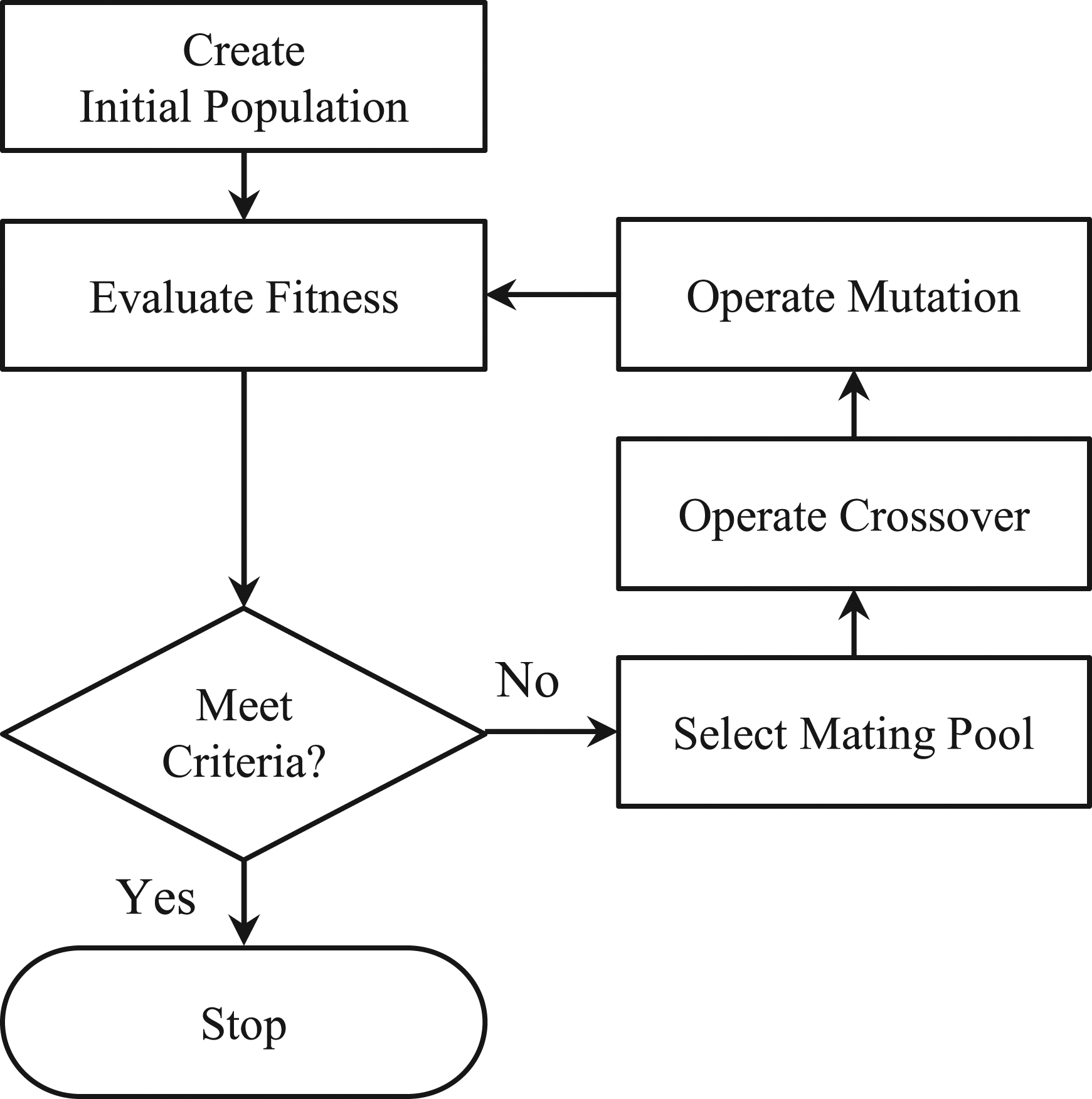

To date, several mutation operators were developed to improve the performance of GAs based on probability distributions. Deep et al. 26–29 proposed two new operators, including the Laplace crossover (LX) and the power mutation (PM), for real coded genetic algorithms. The idea of these operators is to assign a higher probability near the parent individuals when offspring are generated. Michalewicz et al. 30 presented a non-uniform mutation operator that restricts and inherently puts genes in the upper and lower bounds with a uniform distribution. Deb et al. 31 proposed dynamic random mutation, using a random perturbation vector under permissible bounds. On the other hand, gradient-based mutation operators also exist. Bhandari et al. 32 incorporated the simplest gradient information to mutation. Shukla 33 discussed gradient-based stochastic mutation operators. Furthermore, directed mutation was proposed by Quing et al. 34 with the concept of directed variation (DV). Ping–Hung et al. 35 modified DV to adaptive directed mutation for real-coded genetic algorithms. From a review of existing publications, it was observed that simple GAs offer the best performance for large-scale problems; whereas a particular GA with an optimal set of model parameters can provide better performance for mid-scale or small-scale problems. It is worth noting that a tradeoff between the accuracy and the computational cost is required for the optimization problem to be solved.
Adaptive moment optimizer
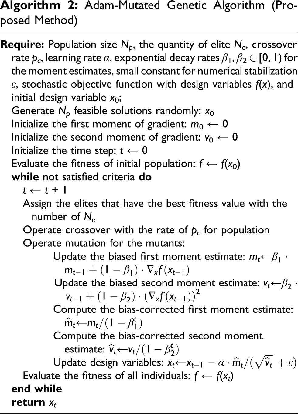
The adaptive moment (Adam) optimizer is a gradient-based optimization algorithm. Adam is devised to maximize performance by regulating the step size, using estimates of the first- and second-moments of the gradients. 36 It has been reported that Adam outperforms other optimizers, such as Adagrad, SGDNesterov, or RMSProp. 37 The pseudo code of the Adam optimizer is presented in Algorithm 1. First, the user should assign the values of the hyperparameters. In accordance with the reference 36 , the learning rate α can be 0.001; the exponential decay rates β 1 and β 2 can be 0.9 and 0.999, respectively; and the small constant for numerical stabilization ε can be 10−8 as a default. The initial values of the first and second moment of the gradients are typically set as zero, while the time step is also set to zero.
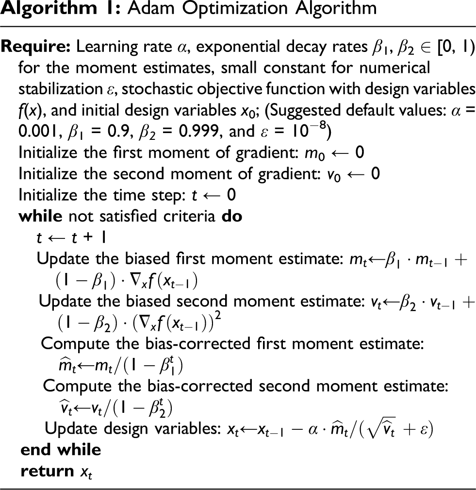
The estimate of the first moment (i.e., mean) is obtained from the exponential moving averages of the gradient. The hyperparameter β 1 determines the accumulating ratio between the previous and current gradient. This idea was inspired from the RMSProp optimizer in that historical search directions are accounted for in determining the current search direction. The estimate of the second moment (i.e., uncentered variance) is the accumulated elementwise-squared gradients that are used in the Adagrad optimizer. The hyperparameter β 2 determines the accumulating ratio between the previous and current squared gradients. The second moment estimate scales the individual dimensions so that design variables move faster for the flattened dimension and slower for the steep dimension. The step size always decreases as the number of iterations increases, since the second moment estimate results in squared positive values. Next, the biases of the two moment estimates are corrected. Finally, the design variables are updated using the bias-corrected first and second moment estimates.
Proposed methodology for sensor network design
This section presents a sensor placement methodology for pipeline systems whose goal is to maximize the detectability of damage. The optimal sensor placement problem can be formulated in a standard design optimization model: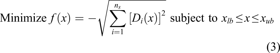
The optimization problem can be considered as a mixed integer non-linear programming (MINLP) problem since the design variables are node numbers in the simulation model. Evolutionary algorithms are one of the possible optimizers that can be used to solve MINLP problems. The quality of the sensor network design depends on the performance of the optimizer. In this paper, the proposed AMGA optimizer is used to solve the problem. The AMGA-based optimizer updates the design variables (i.e., sensor location) until the predefined criterion is met and a final sensor network design is obtained.
The proposed methodology consists of three key blocks, as presented in Figure 2, including statistical database construction, sensor network (SN) design analysis, and SN design update. In the first block, uncertainties in the simulation model are characterized. The probability distributions of pipeline pressures at individual nodes are computed. The computational responses for damage scenarios are recorded to construct a database. In the second block, an initial sensor network design is determined by the user. The predefined number of sensors are placed along the pipeline. The performance of the sensor network design is evaluated using the damage scenario classifier and the detectability metric. In the last block, the sensor placement is updated using the AMGA optimizer until the performance meets the criterion. The sensor network design is finalized when the predefined criterion is met. Details of the three blocks are described in the following subsections. Flowchart for sensor network design using the proposed AMGA optimizer approach.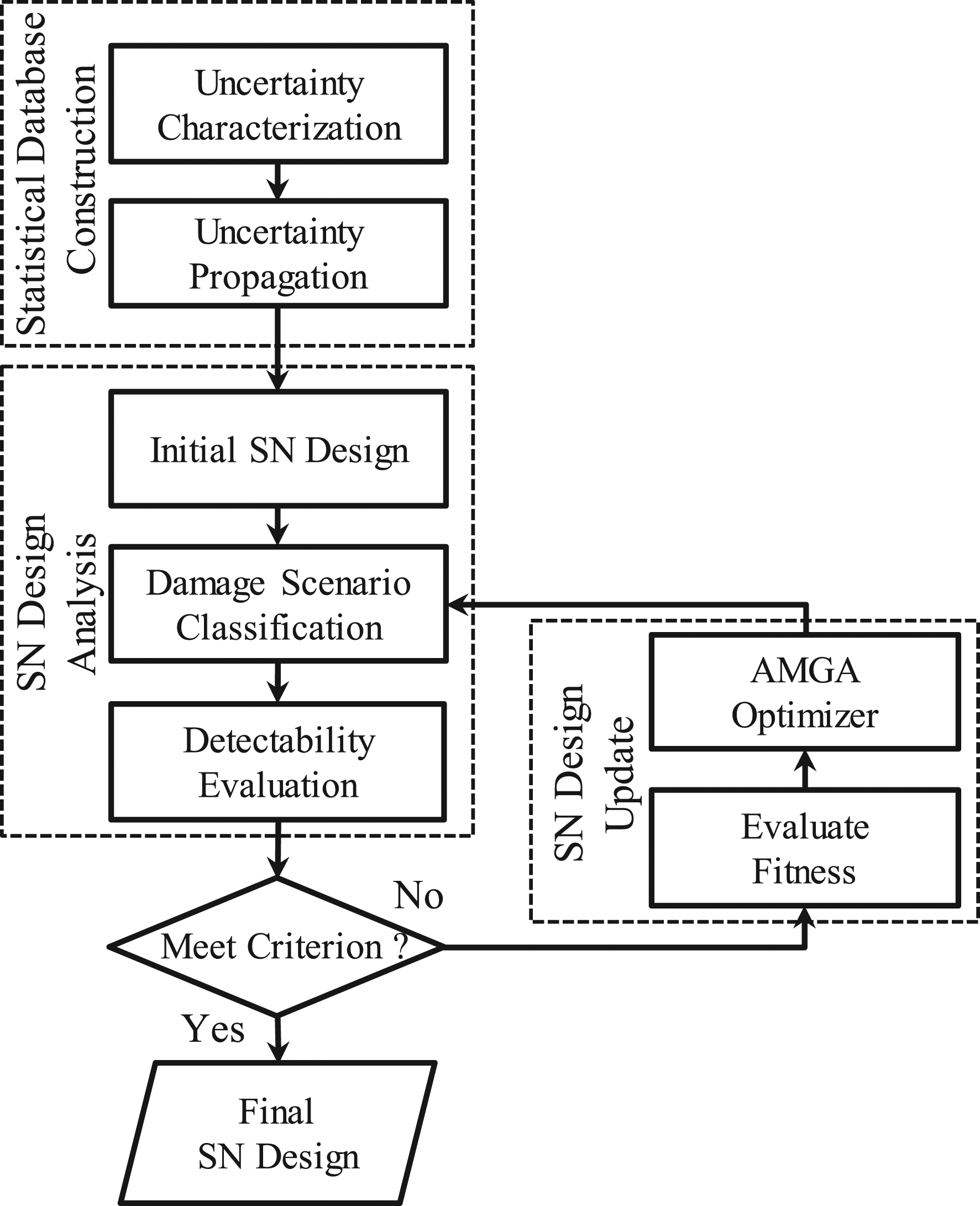
Statistical database construction
Optimal sensor network design is typically conducted for large and complex engineered structures, such as building, bridges, and oil tankers. For these structures, it is practically infeasible to determine the optimal location of sensors by repeated real-world testing (or experiments). With recent advances in computing power, virtual testing using computer simulations is preferred to predict the physical behavior of these structures. As an example, a virtual testing can be conducted to simulate the rupture damage of a fire main pipeline in a naval ship. Three dimensional CAD model of the pipeline system is described in Figure 3(a). A water tank (22 m3) is installed to keep the operating pressure (9 bar) of the pipeline. Two multistage centrifugal pumps (maximum flowrate: 114 m3/hr) are used. The size of the pipe is 150 A. Ten smart valves (SV1∼SV10) were deployed to autonomously detect rupture in the pipeline using two embedded pressure sensors and to isolate the ruptured section of the pipeline. Three damage valves were also installed to represent rupture at three different locations in the pipeline. As shown in Figure 3(b), a real pipeline system was built. It is infeasible to characterize physical behavior (e.g., flow rate and pressure) at any possible location of interest, since sensors cannot be attached due to physical restrictions, such as curved surfaces. To address this challenge, as depicted in Figure 3(c), a simulation model that emulates a real pipeline system was built with open-source software, EPANET, developed by United States Environmental Protection Agency (EPA). The pipeline system consisted of a tank, reservoirs, pumps, relief valves, pipes, and supports. The spots indicated by the nodes correspond to possible locations for sensor placement. Water in the tank is supplied to the pipeline system using the pumps. The relief valves prevent the hydraulic pressure of the pipeline system from exceeding a predefined value. The reservoir is used to save excess water. The pipe supports constrain the six degrees of freedom of the pipeline. Three sites indicated by A, B, and C were the sites for potential damage when external objects hit the pipeline system leading to rupture. The exact location of the rupture sites was determined by domain experts. Pipeline system: (a) 3D drawing, (b) testbed, and (c) simulation model.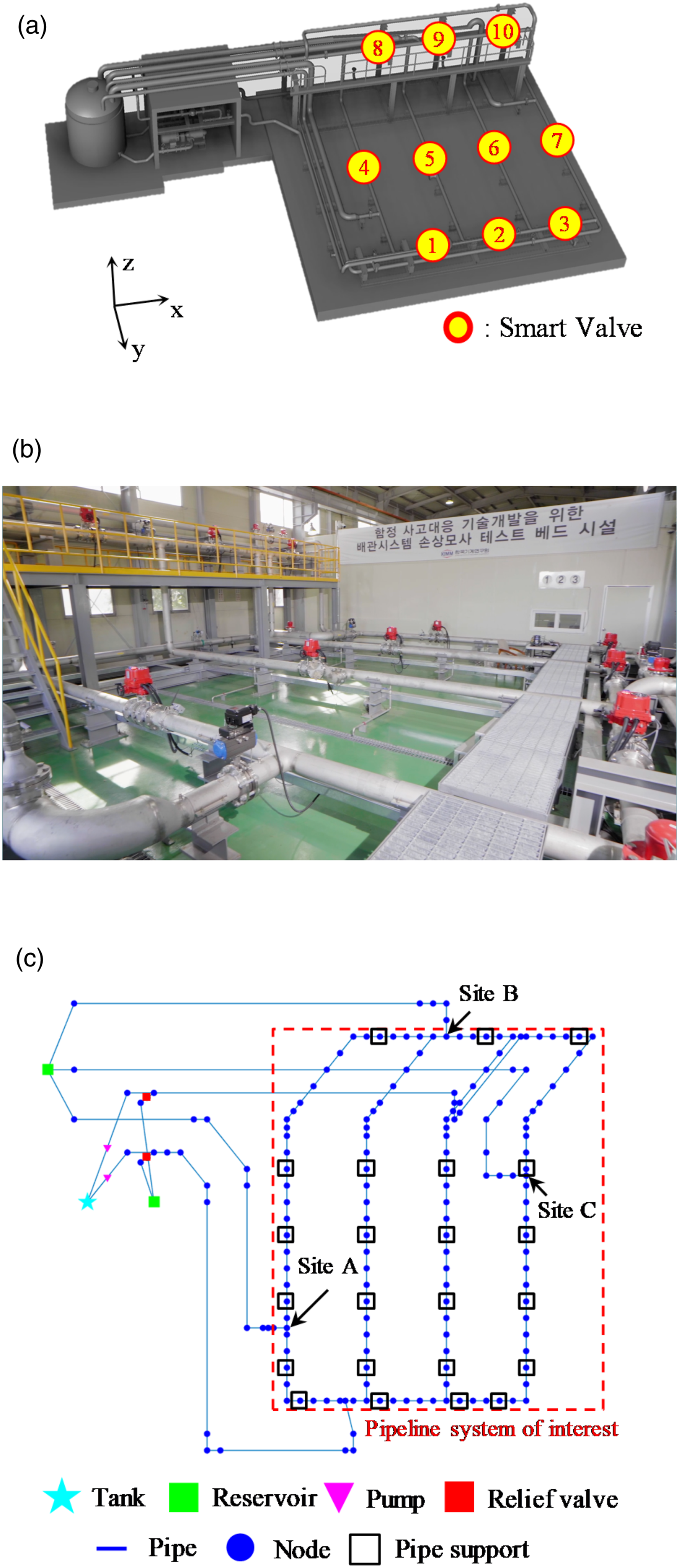
Computational responses from simulations are inherently deterministic; when a single set of deterministic inputs is given, the computer simulation provides a set of deterministic outputs. However, the simulation model can have uncertainty. The simulation model can suffer from model form uncertainty (e.g., the use of a linear model to emulate the nonlinear behavior of a system). The relationship between the true and simulation response can be expressed as:
The inputs can also have uncertainty. For example, physical uncertainty exists due to the manufacturing process (e.g., variations in pipe surface roughness), while statistical uncertainty can arise from insufficient samples (e.g., the use of only three samples to estimate hyperparameters of a normal distribution). The process of quantifying the physical and statistical uncertainty is called uncertainty characterization. The inputs can be expressed in the form of a probability distribution that reflects the physical and statistical uncertainty. Representative examples of uncertainty characterization methods include probability plots, goodness-of-fit (GOF) tests, and kernel density estimation.
The process of obtaining probabilistic simulation responses is referred to as uncertainty propagation. When the uncertainty in the inputs is incorporated during the computer simulations, simulation responses can be obtained in the form of a probability distribution. Uncertainty propagation methods include Monte Carlo simulation, first-order reliability methods, expansion methods, and approximate integration methods. We use the phrase “probabilistic simulation” to indicate the process of having probabilistic simulation responses given uncertain inputs. The outcome (e.g., pressure along the pipeline) from this probabilistic simulation will help estimate the true response from a real pipeline system. For example, as shown in Figure 4, the boxplot of the pipeline pressure at selected nodes can be obtained by uncertainty propagation, considering the physical and measurement uncertainties. Boxplot of pressures at two nodes in the pipeline simulation model.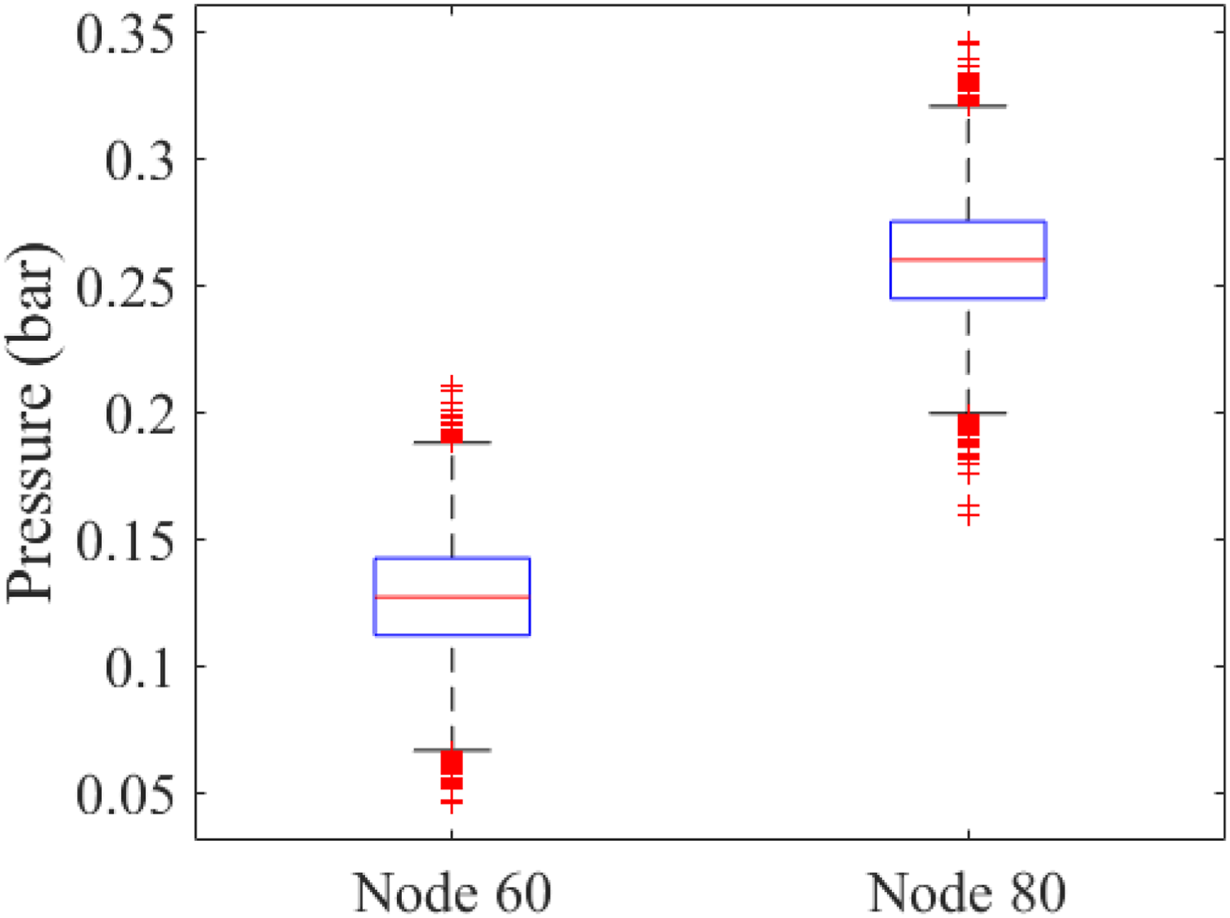
Model validation (or model updating) approaches can be employed to maximize the agreement between the simulation and experimental responses. The simulation and experimental responses are associated with the true responses as follows:
Sensor network design analysis
A sensor network typically requires multiple sensors, depending on the complexity of the target system. As discussed in Statistical database construction, sensor outputs (e.g., pressure) at any location can be calculated using computer simulations for different damage scenarios rather than conducting real experiments. As an example, the pipeline rupture can be attributed to missile attack at the warship front, deck, and end, which correspond to sites A, B, and C in Figure 3, respectively. Damage scenarios with high priority were determined by domain experts. Damage scenarios 1, 2, 3, and 4 were defined as no damage, and damage at sites A, B, and C, respectively. With the damage scenario 1 (i.e., no damage), the pressure in the pipeline was regulated to be nine bars. On the other hand, with the damage scenarios 2, 3, and 4, the pressure decreased from nine bars to the atmospheric pressure (i.e., zero bar for gauge pressure) since the water is drained out. Individual damage scenarios can be simulated by controlling the valves installed at nodes A, B, and C in the simulation model. For example, all the valves are closed for the damage scenario 1, whereas valve A is open instantaneously for the damage scenario 2. The pressure and flow rate at individual nodes of the pipeline can be computed using the pipeline simulation model.
The classification of different damage scenarios will be a trivial problem if the pressure distribution at all the nodes of the pipeline system is known. However, in reality, it is almost infeasible to measure the pressure distribution at all the nodes. Only a limited number of sensors can be placed to measure the pressure at particular nodes. To this end, with a limited number of measurements at particular nodes of the simulation model (e.g., pressure values at two nodes), the damage scenario should be determined. To solve a classification task with multiple damage scenarios, statistical- and machine-learning-based methods have been developed; for example, Mahalanobis distance (MD), 39–41 logistic regression, support vector machine (SVM), 42 artificial neural networks (ANN), 43,44 and convolutional neural networks (CNN). 45,46 In principle, any classifier listed above can be used. In this study, an MD classifier is employed because it is computationally efficient, while allowing consideration of the correlation between input variables with different scales.
MD is a measure of the distance between a point and a distribution. It quantifies how similar a point (i.e., test data) is against a distribution (i.e., training data). The point can be a vector that is defined in a multi-dimensional space. MD is different from Euclidean distance in that MD accounts for the correlation between elements in the vector. The mathematical form of MD is: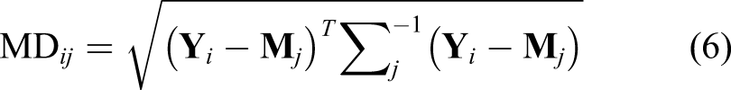
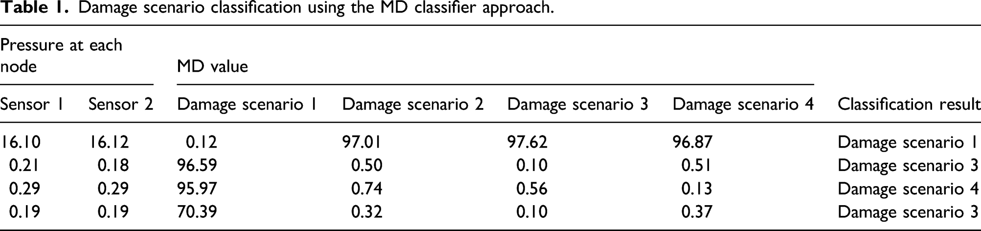
Damage scenario classification using the MD classifier approach.

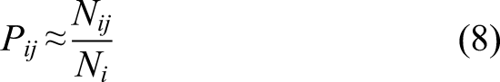
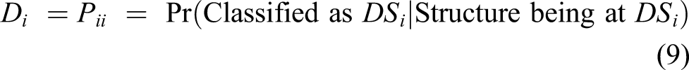
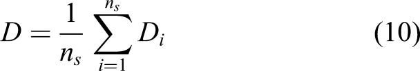
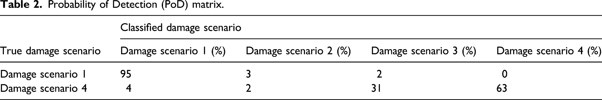
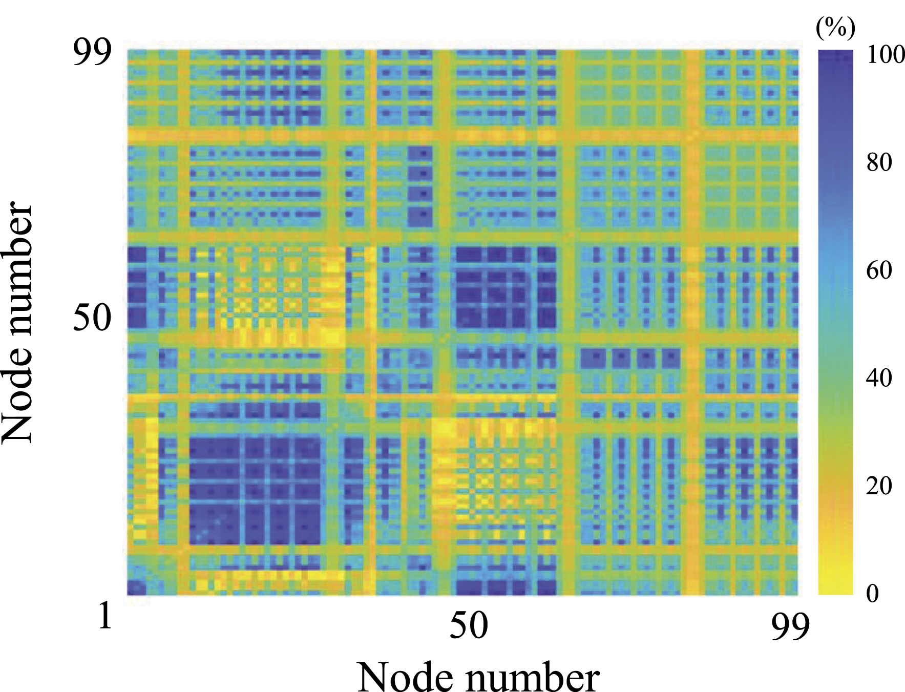
Probability of Detection (PoD) matrix.
Sensor network design update
This section describes the procedure for updating the sensor network design. As presented in Sensor network design analysis, the detectability of the current sensor network design is first evaluated. When the predefined criteria are not met, the current sensor network design should be updated. For updating, an optimization technique can be employed. The optimal sensor network design is a mixed integer nonlinear programming (MINLP) problem, since the sensor location is discretized in the hydraulic simulation model. Genetic algorithms (GAs) are a type of powerful optimizer for solving MINLP problems. In this study, a novel optimizer, namely Adam-mutated GA (AMGA), is proposed and employed. The initial sensor network design is updated with the proposed optimizer until the criterion is met. The details of the proposed AMGA optimizer are described below.
The overall procedure of AMGA consists of six steps, which are identical to those of the standard genetic algorithm (SGA) optimizer, as shown in Figure 1. Among the steps, the mutation operation step (Step 5) is substituted with the proposed method, that is, the Adam-mutation function. The basic concept of the Adam-mutation function is similar to that of the Adam optimizer. In AMGA, the mutation function f m (·) in equation (2) is governed by Adam. The parameter set Θ is defined as the hyperparameters of Adam and the GAs, specifically: (1) the learning rate α, (2) the ratio of accumulating the first moment estimate β 1, (3) the ratio of accumulating the second moment estimate β 2, (4) the small constant for numerical stabilization ε, (5) the population size N p , (6) the quantity of elite N e , and (7) the crossover rate p c . In mathematical expression, Θ = {α, β 1, β 2, ε, N p , N e , p c }. The Adam-mutation function determines the step size and search direction for a given set of parameters and current design variables.
The SN design is updated using AMGA, starting with the randomly generated initial population. The initial first and second moment estimates of gradient are also initialized as zeros. Before the SN design is updated, fitness (i.e., objective function) values for the initial population are evaluated. Among the population, a couple of elite individuals that have minimum fitness values are fixed with the number of N
e
. The crossover operation is implemented for the pairs of individuals selected from the population with the rate of p
c
. The remaining individuals are modified by the Adam-mutation function. The first and second moment estimates are computed using gradients. However, if the mutant individuals were selected as the crossover mates at the previous time step t-1, the two moments for the previous time step do not exist. To address the non-existence of these two moments, a modified gradient is incorporated into the Adam-mutation function. Non-existing gradients at time step t-1 are calculated as follows: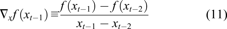
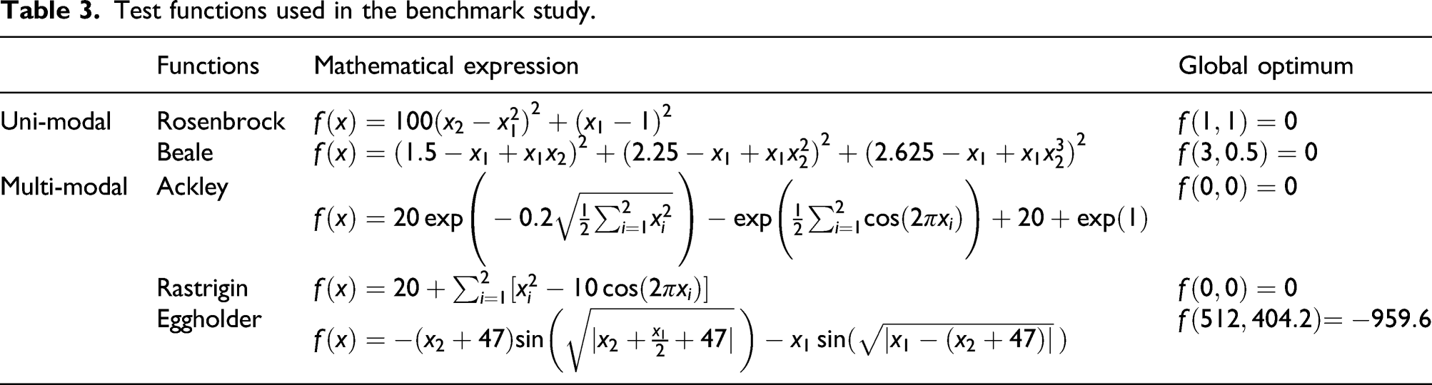
Test functions used in the benchmark study.
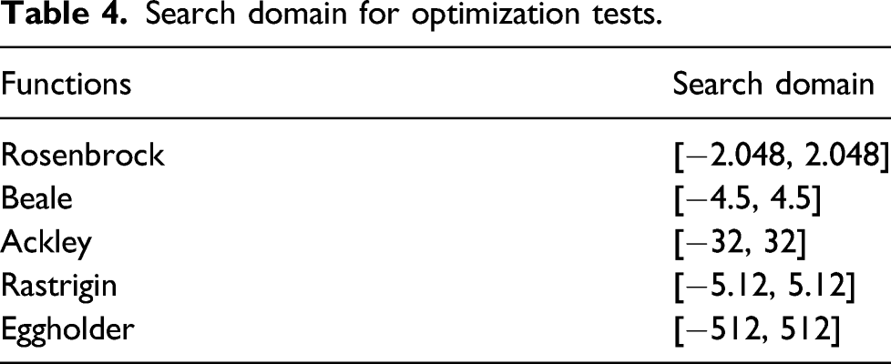
Search domain for optimization tests.
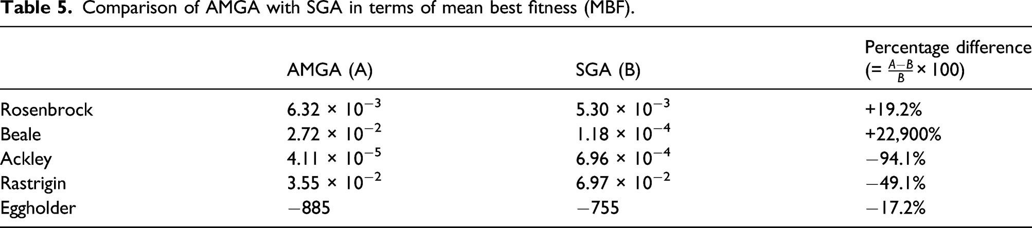
Comparison of AMGA with SGA in terms of mean best fitness (MBF).
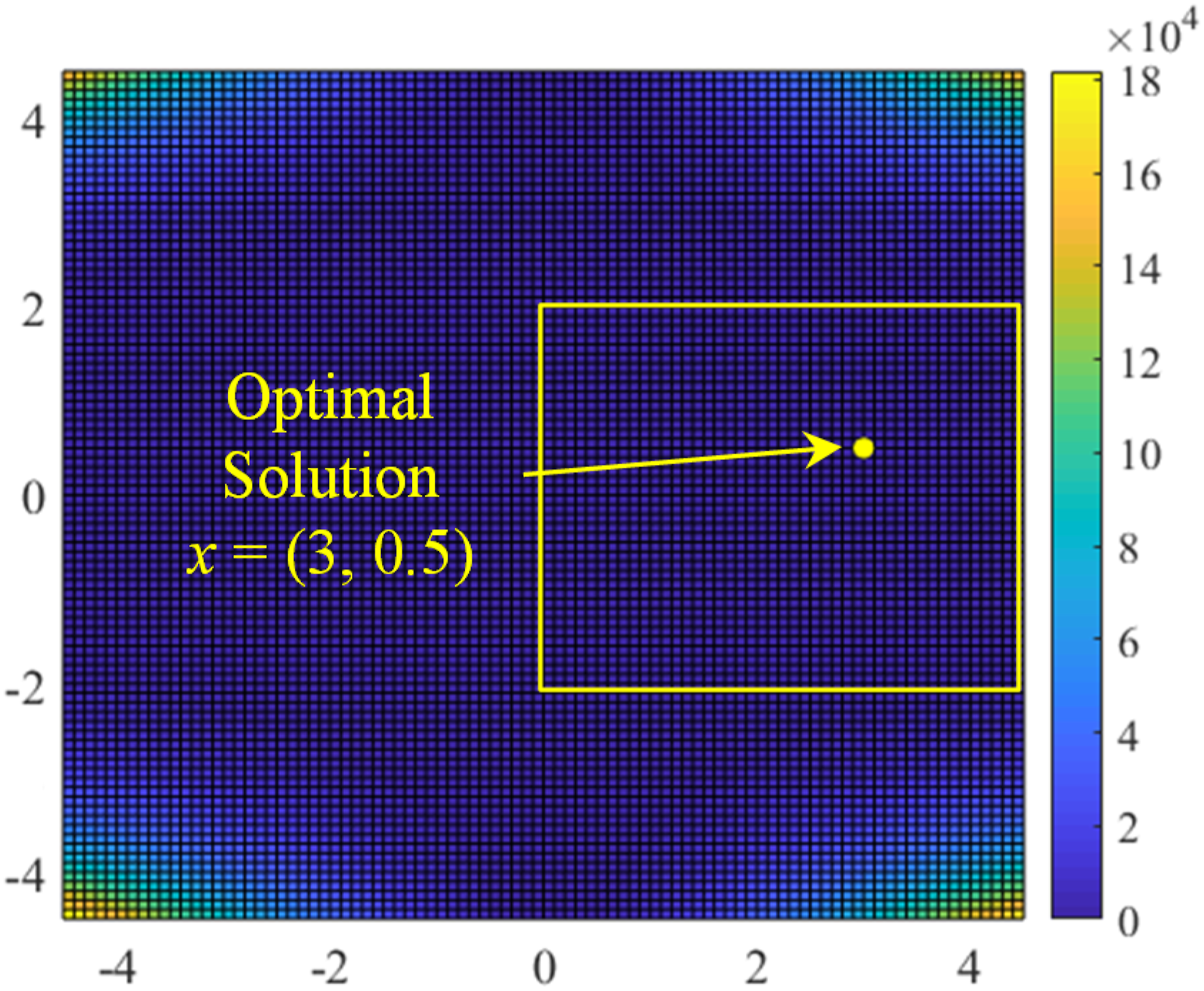
Surface plot of the Beale function with the search space.
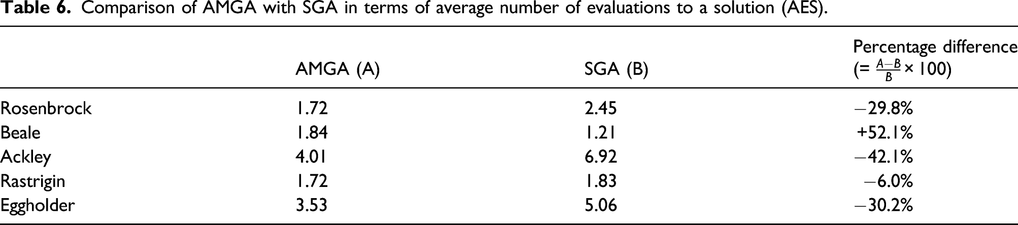
Comparison of AMGA with SGA in terms of average number of evaluations to a solution (AES).
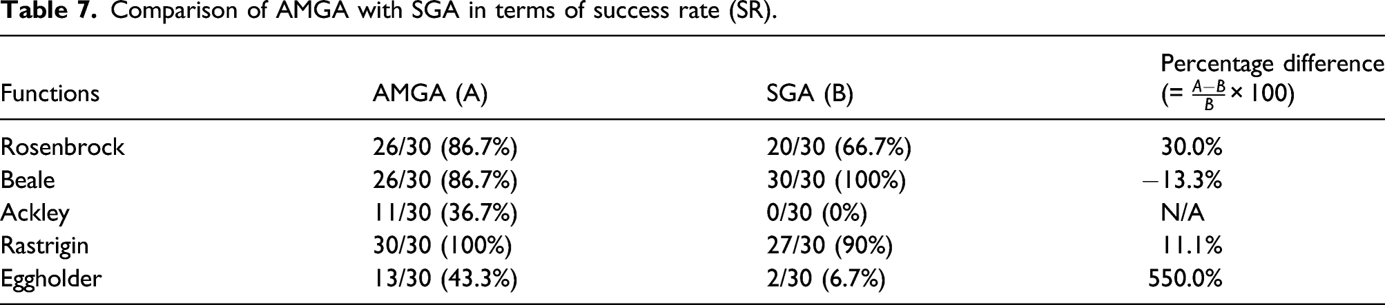
Comparison of AMGA with SGA in terms of success rate (SR).
The performance of the proposed AMGA optimizer was evaluated with unimodal and multimodal test functions in terms of three representative metrics. It was shown that the proposed AMGA optimizer achieved higher performance for the multi-modal functions than the SGA optimizer. Therefore, it was concluded that AMGA can be an effective approach to find optimal solutions to the multi-modal problem.
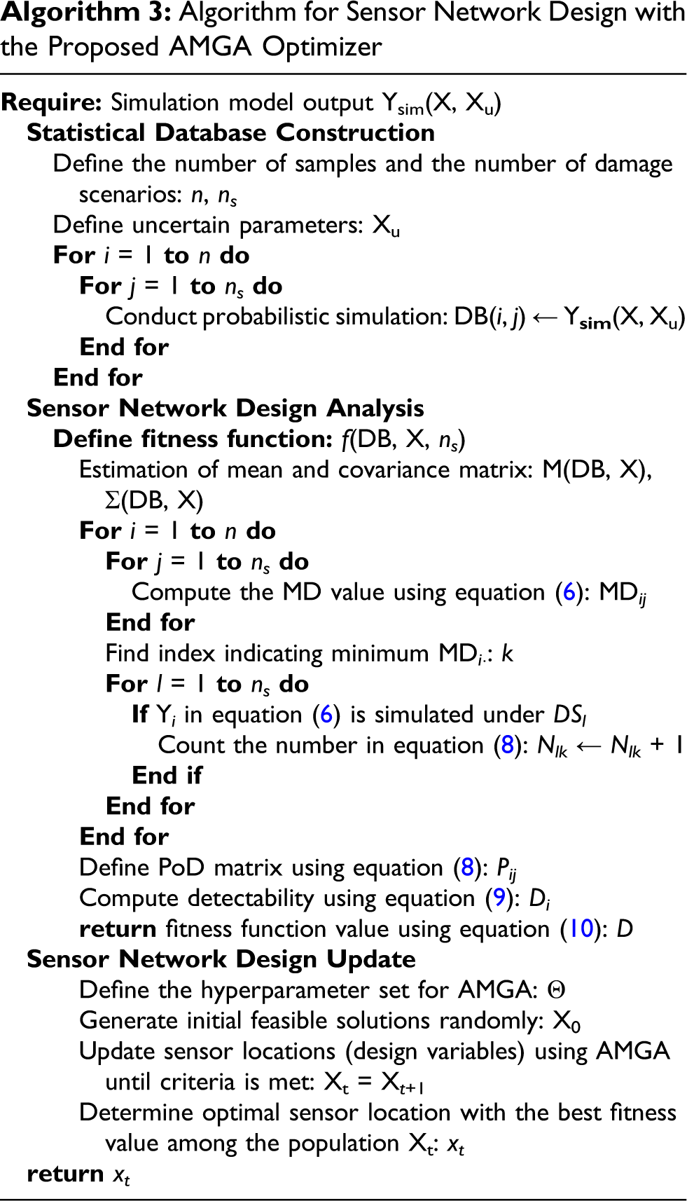
As discussed earlier, the overall procedure of the proposed methodology was summarized in Figure 2. The flowchart consists of three blocks: (1) statistical database construction, (2) sensor network design analysis, and (3) sensor network design update. The pseudo code of the proposed methodology is presented in Algorithm 3.
Case study
A sensor network design problem for pipeline systems is used to demonstrate the effectiveness of the proposed methodology and the AMGA optimizer proposed in this study. For this case study, a testbed was built to emulate a real pipeline system. Using the probabilistic simulation response from a hydraulic simulation model, a database was constructed. The proposed AMGA optimizer was used to find an optimal sensor network. The detectability of the optimal sensor network found by the AMGA optimizer was compared with that found by the SGA optimizer.
Simulation model validation
The simulation model was calibrated using experimental data from the real testbed. Surface roughness and the minor loss coefficient of the pipelines were assumed to be the dominant uncertainty sources. Thus, they were calibrated using a deterministic approach. Details of the calibration of the simulation model are not described, since these details are out of the scope of this paper. For details, see references Oh et al.
38
and Lee et al.
48
After model calibration, the error decreased from 0.0396 bar to 0.0072 bar on average, as shown in Figure 6. It should be noted that the error between the simulation and experimental responses for a smart valve (SV9) was large, compared to those of other smart valves, including SV2, SV5, and SV6. However, the absolute value of the error was 0.03 bar, which was almost negligible. Therefore, it was concluded that the simulation model can emulate the experimental responses. Comparison of simulation responses with experimental responses (a) before model calibration and (b) after model calibration.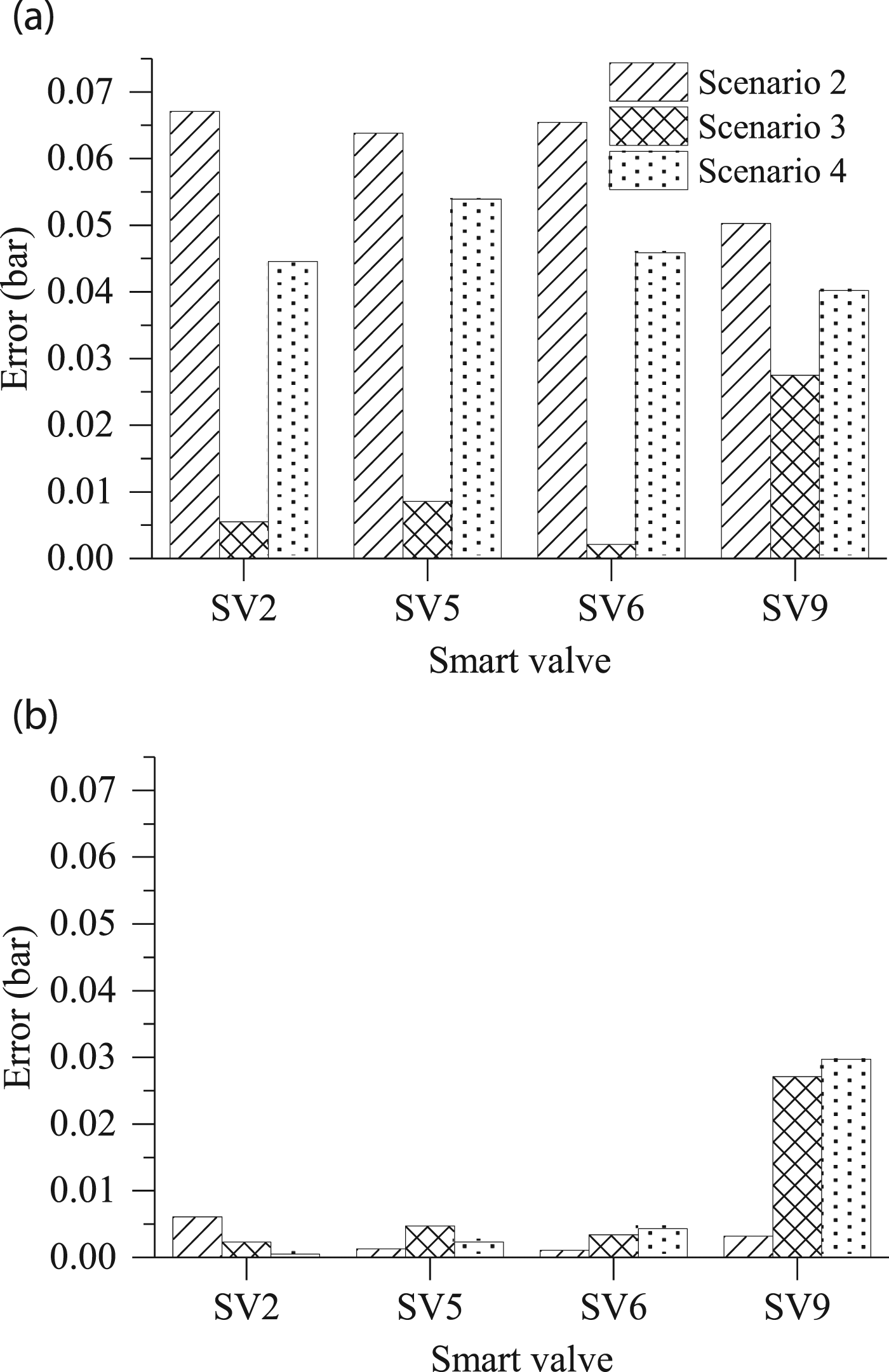
Sensor network design
The proposed methodology for sensor network design was implemented for the pipeline system in the case study. As illustrated in Figure 2, a statistical database of pressure values was constructed using the simulation model of the pipeline system. The simulation model had 99 nodes. The pipe roughness coefficient (R s ∼ N(0.05, 0.005)) and minor loss coefficient (ρ ∼ N(150, 15)) of the pipelines were assumed to be the sources of physical uncertainty, since pipelines are susceptible to corrosion and turbulent flow. The variability from low-cost sensor measurements was assumed to be measurement error. The measurement error was modeled using Gaussian distributions, with a mean of zero and a standard deviation of three different values. In this study, a non-intrusive pipe pressure monitoring sensor, which can be easily installed by clamping outside the pipe was employed. Due to the sensor’s prediction of internal pressure by measuring the diameter change of the pipe, it had different measurement errors, depending on the stiffness of the pipes, as well as the pipe supports. Thus, the standard deviations of the measurement errors were assigned to be 0.0049, 0.02, and 0.03 bar for pipelines with high, medium, and low stiffness, respectively. The stiffness was determined by the distance between the supports and candidate sensor node, as shown in Figure 3(c). For example, a large measurement error with a standard deviation of 0.03 was assigned when the distance between support and node was long.
The uncertainty propagation was conducted by Monte Carlo simulation with 20,000 samples for four individual damage scenarios; the data was divided into sets of 10,000 and 10,000 samples, respectively, for the training and test data. A statistical database with 80,000 sets of pressure values along the pipeline was divided into training data of 40,000 sets and test data of 40,000 sets. For individual scenarios, pressure values at nodes were recorded. As an example, for Damage Scenario 2, the pressure values for Nodes 60 and 80 can be visualized by a boxplot, as shown in Figure 4.
An initial SN design was determined by randomly selecting sensor nodes with the predefined quantity. Using the training set, pressure values for the selected nodes are used to calculate the mean and covariance matrix of the MDs for individual damage scenarios. Using the test set, MD values were computed for individual damage scenarios. For instance, when the initial sensor network was designed with Nodes 72 and 94, the PoD matrix was obtained as: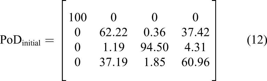
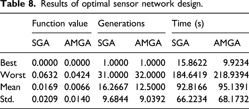
The optimization problem was formulated as an MINLP problem to account for the discretized sensor node selection. The quantity of candidate sensor nodes was 99, as depicted in Figure 3(c). Therefore, 99C N number of sensor network designs is possible, where N is the number of nodes for sensor placement. If N is two or three, the possible combinations of the sensor nodes are 4,851 and 156,849, respectively. The computational time increases exponentially as the number of nodes increases linearly. Exhaustive search is feasible when the number of the candidate sensor nodes is small. However, if a simulation model of a real scale with a large number of candidate sensor nodes is employed, it is almost infeasible to compute the detectability of all candidate sensor networks. To address this challenge, an evolutionary algorithm can be used. In this study, the proposed Adam-mutated genetic algorithm was used as an optimizer. The hyperparameters Θ = {α, β 1, β 2, ε, N p , N e , p c } were set as α = 0.001, β 1 = 0.9, β 2 = 0.999, ε = 1×10⁻⁸, N p = 50, N e = 3, and p c = 0.8 in this study. The quantity of sensors was set to be two. The termination criteria were the maximum generation of 100 and the maximum stall generation of 20. In the first step, 50 SN designs were selected randomly. The sensor network designs were updated over 12.5 generations and, on average, optimized by the AMGA optimizer 30 times.
Results and discussion
Different from the statistical approach described above, the deterministic approach does not consider uncertainty sources, such as physical variations and measurement errors. In the deterministic approach, the pressure values for individual damage scenarios were calculated using the EPANET hydraulic simulation model, as shown in Figure 7. The horizontal axis indicates sensor node numbers, while the vertical axis represents pressure values for individual nodes. It will be desirable to place a sensor at the nodes with the largest pressure differences between individual damage scenarios. As an example, when a sensor was placed at Node 29, damage scenarios 2 and 4 could be distinguished by setting a hard threshold. However, as expected, damage scenarios 2 and 4 are distinguished if the effect of measurement errors on true pressure values is large compared to the pressure difference. Using the deterministic approach, the two sensor locations were determined to be Nodes 29 and 65. However, the deterministic approach cannot account for uncertainty. As an alternative, the probabilistic approach is incorporated with the probabilistic performance measure, that is, detectability. Nominal pressure values along the pipeline.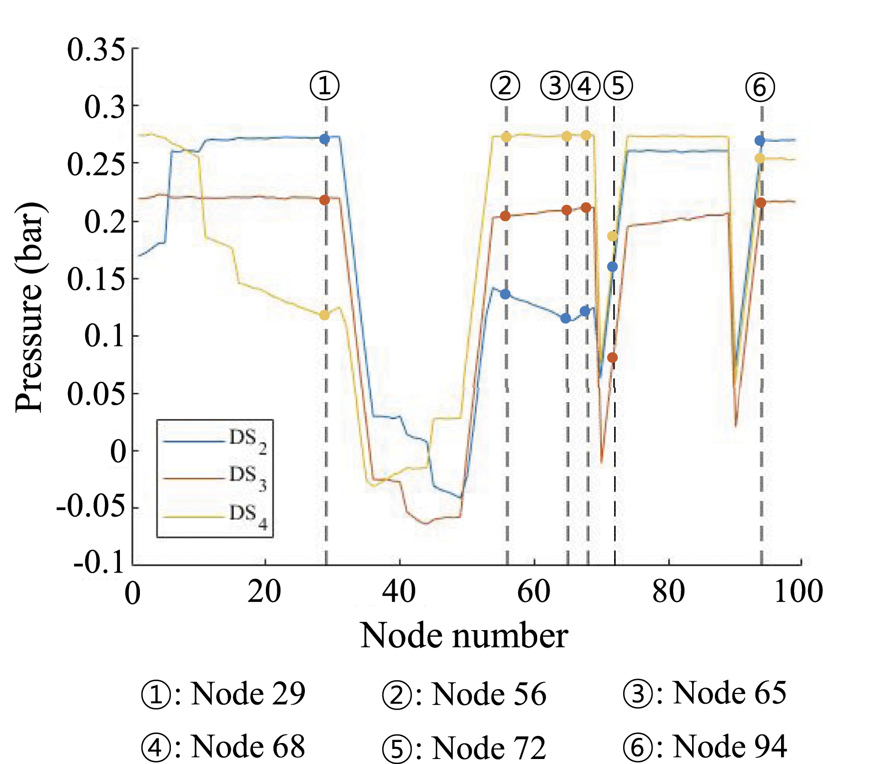
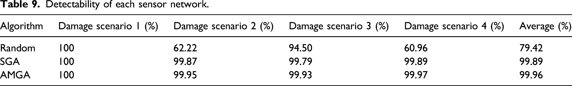
An optimal sensor network was designed using the proposed Adam-mutated genetic algorithm (AMGA). The pressure values acquired by sensor placement at Nodes 56 and 68 are described in Figure 8. As shown in Figure 8(a), when the pressure is measured at Node 56, pressure distributions can be calculated. For the individual damage scenario, the pressure values are distributed due to the uncertainty including physical variations and measurement errors. Nevertheless, three pressure distributions that correspond to damage scenarios 2, 3, and 4 do not overlap. This indicates that a potential damage scenario can be determined accurately, when a sensor is placed at Node 56. A single sensor placement can be sufficient to determine the damage scenario. When the number of sensors is increased, the classification accuracy can be improved. For the very reason, another sensor is placed at Node 68. As described in Figure 8(b), the pressure distributions do not overlap. To visualize the pressure distributions at Nodes 56 and 68 together, a two-dimensional scatter plot is used as presented in Figure 8(c). It is worth noting that damage scenarios 1, 2, 3, and 4 are plotted in the scatter plot. The clusters did not show any overlap for individual damage scenarios. When two sensors were placed at Nodes 56 and 68 with the proposed methodology in this study, the detectability of 99.96% was achieved on average. Optimally designed sensor network: (a) pressure distribution at Node 56, (b) pressure distribution at Node 68, and (c) 2D scatter plot at Nodes 56 and 68.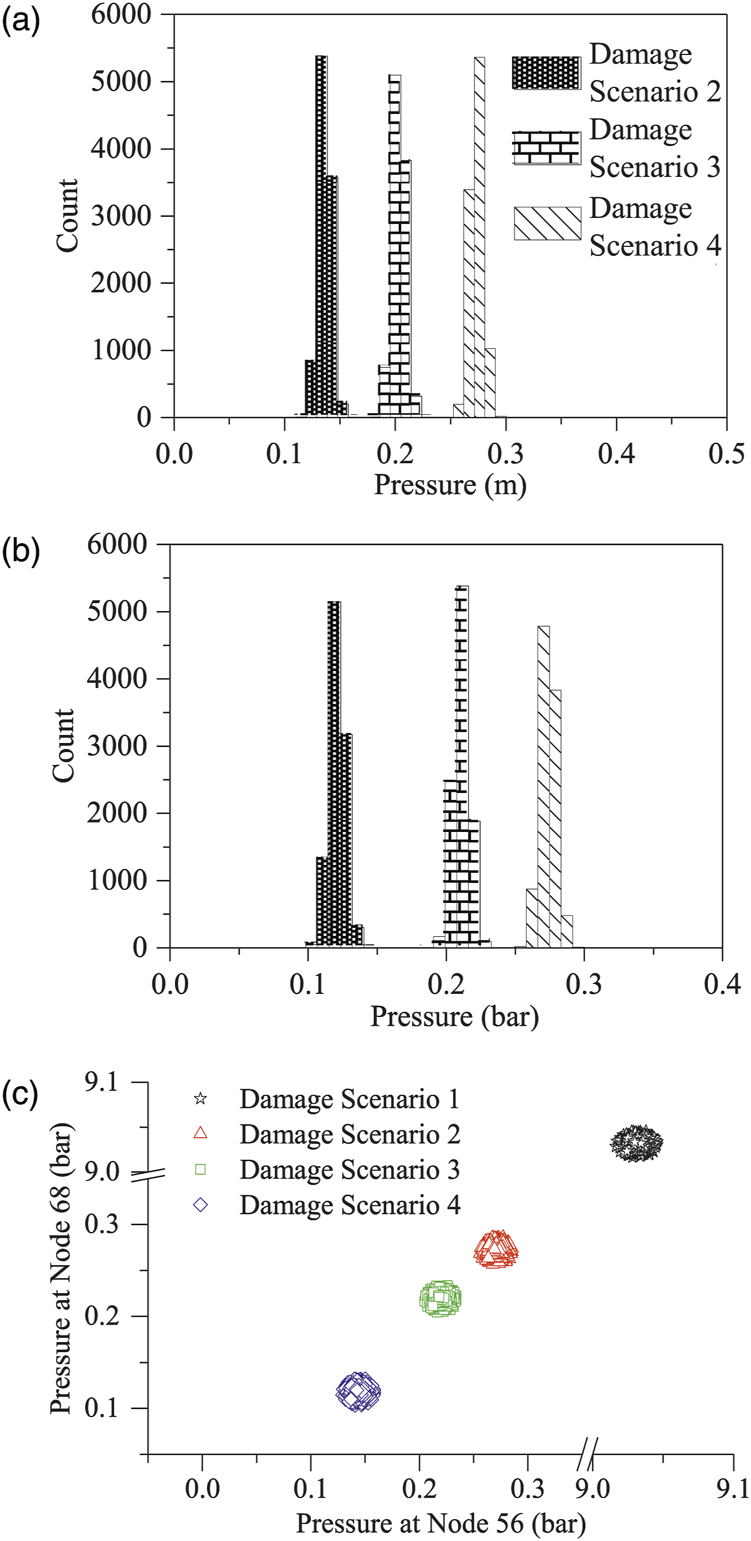
To compare the detectability, a sensor network was designed by selecting two nodes arbitrarily: Nodes 72 and 94. The detectability was as low as 79.42%. As presented in Figure 9(a), when the sensor is placed at Node 72, the pressure distributions overlap between damage scenarios 2, 3, and 4. The damage scenario 2 and 4 cannot be classified due to variations caused by the uncertainty. This is true when another sensor is placed at Node 94 as shown in Figure 9(b). When the sensor location was not optimal, additional sensor placement did not help increase the detectability. As presented in Figure 9(c), damage scenarios 2, 3, and 4 were still difficult to separate due to the overlap. Sensor network design with arbitrarily selected sensor nodes: (a) pressure distribution at Node 72, (b) pressure distribution at Node 94, and (c) 2D scatter plot at Nodes 72 and 94.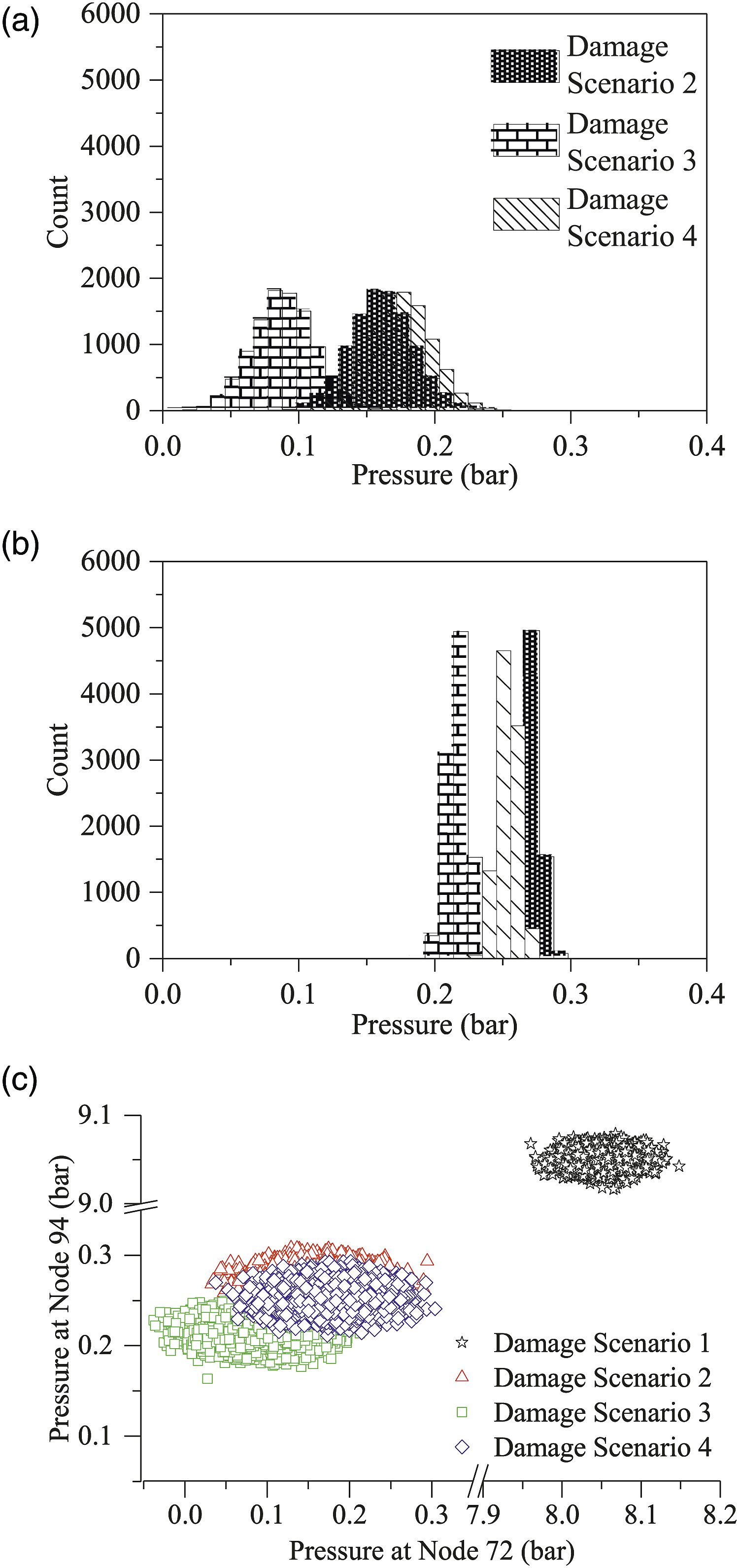
Results of optimal sensor network design.
Detectability of each sensor network.
Multi-modality spanned sensor network design optimization problem.
Conclusions
This paper presented a novel methodology that determines the optimal location of sensors in a pipeline network for real-time monitoring. The proposed methodology consists of three main steps: (1) statistical database construction, (2) sensor network design analysis, and (3) sensor network design update. In particular, for the sensor network design update, a new optimizer, that is, Adam-mutated genetic algorithm (AMGA), was proposed. The performance of AMGA was evaluated with unimodal and multimodal test functions. With the evaluation metric of mean best fitness (MBF), AMGA outperformed the standard generic algorithm (SGA) by 17.2%–94.1% for multimodal functions. The average number of evaluations to a solution (AES) of AMGA was superior to SGA by 6%–42.1%. The success rate of AMGA was 11%–550% higher than that of SGA. From the benchmark study, it was corroborated that the proposed AMGA optimizer was efficient and accurate to find optimal solutions for multimodal functions. Then, the new AMGA optimizer was incorporated into the proposed methodology for sensor network design. Finally, the proposed methodology was evaluated with the case study of the real pipeline system. When two sensors were placed with the proposed methodology, the detectability of 99.96% was achieved on average. With the SGA optimizer, the detectability was 99.89% which was comparable to that of the AMGA optimizer. However, the function value and generations of AMGA were superior to those of the SGA optimizer. The worst case scenario was also evaluated. When two sensors were placed randomly, the detectability was as low as 79.42%. The random placement of additional sensors did not necessarily increase the detectability.
This paper devised the new AMGA optimizer to solve sensor network design optimization problem formulated as a mixed integer nonlinear programming (MINLP). For the small-scale and multi-modal problem in the case study of this paper, it was corroborated that the AMGA optimizer performed as accurate as the SGA optimizer. It should be noted that AMGA outperformed in terms of function value and generations. From the observations, it is anticipated that the proposed methodology, which employed the AMGA optimizer, can be used for sensor network design of large-scale ships as well as infrastructures, such as petrochemical plant pipeline systems, for real-time monitoring.
This study has a couple of limitations that require future study. First, the computational costs of current methods can be very expensive when the search space is extremely large. The proposed methodology does not resolve the curse of dimensionality problem, although AMGA can relieve the problem by finding sub-optimal solutions. Second, the responses from the hydraulic simulation model used in this study, so called EPANET, can deviate from the experimental results. The validity of the simulation model should be improved further to obtain the accurate pressure and flowrate of water in the pipeline system.
Footnotes
Declaration of conflicting interests
The author(s) declared no potential conflicts of interest with respect to the research, authorship, and/or publication of this article.
Funding
The author(s) disclosed receipt of the following financial support for the research, authorship, and/or publication of this article: This study was supported by National Research Foundation of Korea, 2021R1A2C1008143; Korea Institute of Machinery and Materials, NK213E.