Synthesis of healthy-structure model responses for damage quantification

Abstract

Structural Health Monitoring faces several challenges. Among them, especially for the quantification of damage, are (1) the uncertainty in the boundary conditions, (2) the need for a calibrated numerical model, or measurements, of the structure in its healthy state, (3) the variability in the structure properties and boundary conditions due to environmental and operational conditions and (4) the possibility of damage in the virgin structure due to construction defects. Based on the sparsity condition of structural damage, this work presents a method that tackles these challenges simultaneously. The method consists in synthesising the response of a healthy-structure model, which is valid in the current environmental and operational conditions, only inside a region of interest (ROI) that excludes the boundaries and the rest of the full structure. This is accomplished by means of a robust regression of the solution of an analytical model of the healthy structure, and its loading, only using testing data of the (possibly) damaged structure in that ROI. Under ideal conditions, the method showed to be exact in detecting, locating and quantifying damage, in some cases much better than using measurements of the virgin structure. Finally, the method was tested by numerical simulations and using experimental data, under realistic conditions, which evidences its practical applicability.

Keywords

Damage quantification boundary conditions healthy state model synthesis robust regression damage sparsity

Introduction

Structures might silently accumulate damage throughout its life cycle. This damage can be a serious issue, especially when a partial or total unexpected collapse might occur. For its obvious importance, an enormous number of papers and books have addressed methods under the general term of Structural Health Monitoring. These methods can output different information. In this regard, Rytter¹ distinguishes four levels:

Level 1: Detection. The method gives a qualitative indication that damage might be present in the structure.

Level 2: Localisation. The method gives information about the probable location of the damage.

Level 3: Quantification (assessment). The method gives information about the size of the damage.

Level 4: Consequence. The method gives information about the actual safety of the structure given a certain damage state.

Usually, levels 1 and 2 can be reached using heuristic and/or meta-heuristic approaches, such as novelty detection,^2,3 local modal filters⁴ and natural frequency ratios.⁵ These methods are very attractive, especially for complex structures, since they do not rely on detailed mathematical models but on simple assumptions, for example, ‘the structure model behaves as linear’ or ‘the occurrence of damage and the change in environmental or operational conditions are not correlated’. Thus, the variability due to those conditions can be filtered out statistically² or using properties derived from linearity.^4,5

On the other hand, for reaching levels 3 and 4, two mathematical models, that of the (possibly)¹ damaged structure and that of the healthy structure, are usually required. This is because damage is commonly defined as a local reduction in stiffness, so current and reference stiffnesses must be compared. In the words of Rytter,¹ the healthy-structure model requires a virgin state calibration using virgin state measurements. The requirement for virgin state measurements is really problematic for several reasons, some of which are rarely mentioned in the literature. Starting with the obvious, the structure may have gone through much of its life cycle without performing measurements on it. It is also possible that virgin state measurements are available; however, boundary, environmental and/or operational conditions may have changed. The change in boundary conditions is a particularly important issue, since it can be the main damage, as studied by Park et al.,⁶ or a harmless environmental effect, for example, Alampalli⁷ reported that the relative eigenfrequency differences of a bridge due to freezing of the supports were an order of magnitude larger than changes due to damage. Other less noticed problems are the following.

Components of the measurement system are very likely to change during the life cycle of the structure, either by maintenance or obsolescence. Since noise-to-signal ratios and sensor alignments may have changed, current and virgin state measurements are not comparable directly. Other problem is behind the commonly accepted definition of virgin state measurements: that is, those performed ‘immediately after the ending of the construction work’.¹ Therefore, if construction defects are present, quantifying damage by taking the virgin state as reference can be misleading. This is easily overcome in mass-produced parts by carefully selecting the reference specimen; although such a selection is not possible in unique parts of many civil structures.

An alternative for quantifying damage without using virgin state measurements, usually called model updating, consists in solving an inverse problem where individual properties of small regions of the structure, for example, element stiffnesses in a Finite Element (FE) model, are calibrated taking measurements as reference. The direct statement of this inverse problem is usually ill-posed because of the number of unknowns, especially for large and complex structures. The traditional approaches to tackle this are assuming damage scenarios⁸ or using regularisation techniques.^9–11 Both are based on assuming the sparsity of damage. However, model updating is still computationally demanding. More importantly, the development of a model including damage scenarios can become very laborious if the structure is large and complex, and/or the available information is incomplete.

Other approach to deal with the ill-posedness of inverse problem-based damage quantification consists in isolating a region of the structure using, first, a damage detection and localisation technique. For example, He et al.¹² employed the gapped smoothing method to locate the edges of damage in beams from the vibrational curvature data, followed by an inverse method to determine the through-thickness location of delaminations.

For the case of simple structures with unknown boundary conditions, Pitchai et al.¹³ presented mechanics-based algorithms to quantitatively determine the current state of a bridge using quasi-static loading and strain measurement: one for determining end rotational restraints of a beam segment and other for determining its material properties. These algorithms are interesting as they are not based on optimisation problems; however, they are applicable to prismatic beams only instrumented with strain gauges.

Regarding measurement techniques, computer vision has shown to be a promising approach, particularly when combined with statistical analysis. For example, Zaurin and Catbas¹⁴ used correlated images and sensor data (strain, acceleration and tilt) to create a series of unit influence lines, which are used as input features to detect and localise damage in the structure. This method was also capable of quantifying damage but, as usual with statistical approaches, only in a relative sense.

Another attractive sensing technique involves the use of a scanning laser vibrometer. In this context, Zaurin and Catbas¹⁴ interrogated local operating deflection shapes by means of two-dimensional directional Gaussian wavelets for damage. Results showed that the method is capable of revealing directional features of small damage with high precision and strong robustness against noise. Interestingly, since the method has a local property, it requires no numerical or physical benchmark models for the entire structure in question nor any prior knowledge of either the material properties or the boundary conditions of the structure. However, damage quantification was not mentioned.

The important concept here is that virgin and healthy are not equivalent terms in general. Virgin is the state in which the structure was just after its construction, while healthy is the state in which the structure should be.

In order to overcome the problems related to the virgin state measurements, in this work, it is proposed not to use them at all. Instead, the healthy-structure model (HSM) is defined as ‘that presumably used to design the structure’ (rather than ‘that representing the structure as constructed’). That is, it is a model of a fictitious structure. In particular, the (geometry, material and load magnitude) parameters of the HSM are those satisfying some operational and environmental conditions such that the resulting internal forces are the same as those of the current structure (rather than those parameters satisfying the conditions of the structure just after its construction). Also, the HSM only needs to be defined in a region of interest (ROI) that excludes the boundaries of the full structure.

On the other hand, the healthy-structure model response (HSMR) is defined in this work as ‘the solution of the differential equation of the HSM with some new boundary conditions such that the resulting internal forces are the same as those of the current structure’ (rather than with the boundary conditions of the structure just after the construction). More important, to synthesise the HSMR, it is not necessary to know those new boundary conditions, knowing their corresponding integration constants is sufficient.

These two definitions are very convenient for three reasons: (1) construction defects can be addressed; (2) many complex structures can be piece-wise represented with simple analytical models, if they are healthy in the sense here defined; and (3) the inverse problem of finding the HSMR can be well-posed using little information.

All of this leads to the following simple and robust method for damage detection, localisation and, more importantly, quantification.

In the event that the healthy structure cannot be measured, the HSMR can be synthesised. The available tools to conduct such syntheses are (1) the measurements of the damaged structure and (2) the HSM in the ROI (including a representation for the loading) with n_ip unknown parameters called hereinafter internal parameters. On the other hand, the HSMR depends on those internal parameters but also on n_epexternal parameters, that is, the integration constants associated with the boundary conditions that the rest of the structure imposes to the ROI. All those n_ip + n_ep parameters can be found by means of robust regression on the response, using the damaged structure measurements as data points, if damage is assumed to be sparse. This is the key idea of the method here proposed. Details of this synthesis and how it is then used to quantify damage are given in the following sections.

Comparison of the proposed method with other similar methods

Before proceeding with the details of the method, it is convenient to remark the differences between this and similar ones found in the current literature.

The Gapped Smoothing Method (GSM), originally proposed by Ratcliffe,¹⁵ is a popular technique that relies on the assumption that the healthy structure has a smooth mode shape curvature that can be approximated by a low-order polynomial. Such a polynomial is fitted ‘for each element in turn, with the coefficients being determined from the data on either side of the current element, but excluding it’.¹⁵ Then, a damage indicator is constructed as the difference between the measured and fitted mode shape curvatures, which allows detecting and locating damage. This idea was later extended by Yoon et al.¹⁶ They presented the Global Fitting Method (GFM), which also defines the damage indicator as a difference of curvatures, but more points are used and the generic form of the mode shapes of a healthy beam is used as the fitting function. In the present work, a more general mechanics-based mathematical justification is given for the construction of the particular function to be fitted, and the way in which it is convenient to perform that fitting (robust regression instead of multiple fittings or least-squares global fitting). This allows defining a damage indicator that is not only capable of detecting and locating damage but also of quantifying it.

For its part, sparse identification was successfully used to establish a baseline (healthy) model for damage detection and characterisation in a recent work.¹⁷ However, a structure that behaved as undamaged (due to low excitation level) was used therein. Conversely, the present paper will show the important fact that a structure exhibiting damage in its response can also be used for synthesising an accurate baseline model, under the assumption that damage is sparse.

As stated in ref. 18: ‘the central difference approximation employed in most of existing studies needs appropriate spatial resolution to obtain accurate curvatures’. Therefore, the possibility of quantifying damage with independence of sensor separation is of major importance. Particularly, it is desirable to be able to quantify damage using few and separated sensors, since that relaxes measurement accuracy requirements before differentiation. Such a possibility was recently introduced in ref. 19 for simply supported beams. There, it was assumed that the bending moment remains approximately constant after damage (hence the simple support condition). Instead, the method here proposed assumes that there exists a fictitious healthy beam with exactly the same bending moment as the damaged beam. This new assumption extends the practical applicability of the method to one-dimensional structural members belonging to an arbitrary structure.

Finally, it is worth to say that the idea of solving the analytical model of a healthy beam, instead of using virgin state measurements, has been previously used by El-Gebeily and Khulief²⁰ for the identification of wall-thinning and cracks in pipes. In that work, the bending stiffness reduction was quantified with the quotient of two curvatures: (1) measured and (2) analytically solved assuming known boundary conditions and known nominal values of the beam. Moreover, only the case of a simple supported beam was discussed. On the contrary, the method proposed in the present paper achieves more broad applicability in practice since boundary conditions can be of any kind and need not to be known, which is ideal for beams and bars being part of complex structures. Besides, nominal values as stiffness and mass distribution need not to be known; only their (dimensionless) shapes along the member axis are required. This is particularly useful for materials with uncertainty in the global elastic modulus and global mass density (e.g. 3D printed plastics) and for structural members whose cross-section has undocumented and inaccessible inner-geometry.

Definitions

Definitions of internal deformation, -force and -stiffness

For simplicity, only one-dimensional structural members are addressed in this work, which can belong to a general structure as shown in Figure 1. The longitudinal axis is named as x; and the vector fields of displacements, axial and shear forces, and bending moments in the ROI are named as [u_x(x) u_y(x) u_z(x)], [F_x(x) F_y(x) F_z(x)] and [M_x(x) M_y(x) M_z(x)], respectively. The set of values of x belonging to the ROI is named as D_ROI.

Figure 1.

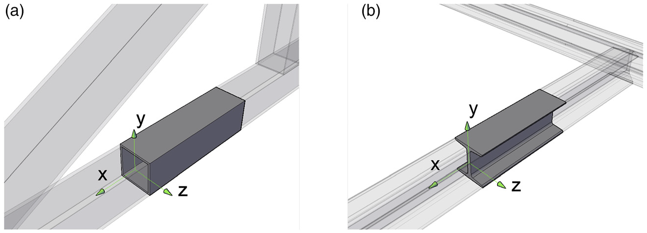
Coordinates for (a) bar and (b) beam segments, being part of a structure.

Here, the internal deformation d_i(x) is a generalisation defined as a size change that is related to the damage under consideration. For example, if damage is being assessed in a bar, internal deformation is the derivative of axial displacements, that is, the resultant of the axial strains $d_{i} (x) = u_{x}^{'} (x)$ . In the case of a beam², it is the curvature of one of the transverse displacements $d_{i} (x) = u_{y}^{''} (x)$ .

The internal force f_i(x) is a generalisation defined as the function that forms a conjugate pair with the internal deformation, that is, the product f_i(x)d_i(x) is the deformation energy per unit length associated to the damage under consideration. For the case of a bar, the internal force is the resultant of the axial stresses in the bar cross-section, that is, the normal force f_i(x) = F_x(x). For a beam, the internal force is the bending moment f_i(x) = M_z(x).

In this work, the internal stiffness is defined as the quotient

k_{i} (x) = \frac{f_{i} (x)}{d_{i} (x)}, x \in D_{ROI}

(1)

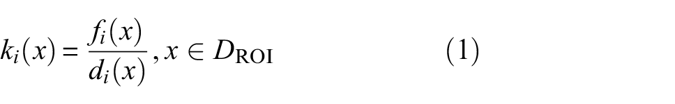
and it will be used to quantify damage. Note that k_i(x) is a generalisation of EA(x) (bar) and EI(x) (beam). Similar deductions can also be made for shear and torsion.

Definition and quantification of damage

For simplicity of notation, d_i(x), f_i(x) and k_i(x) refer to the (possibly) damaged structure, while d_ih(x), f_ih(x) and k_ih(x) refer to the healthy structure.

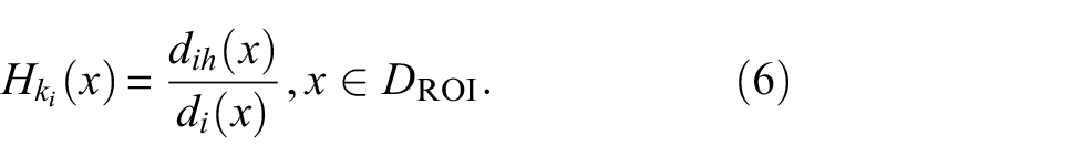
As in ref. 19, damage at x is quantified in this work using the health index

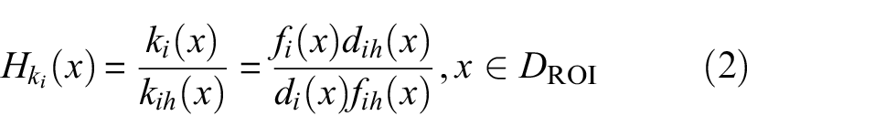
H_{k_{i}} (x) = \frac{k_{i} (x)}{k_{ih} (x)} = \frac{f_{i} (x) d_{ih} (x)}{d_{i} (x) f_{ih} (x)}, x \in D_{ROI}

(2)

which ranges from 0 (total loss of stiffness) to 1 (healthy case).

Assumptions

As any other damage identification method, this also relies on assumptions. The purpose of this section is to explicitly put them in sight for the convenience of potential users.

Invariability of the internal force

The proposed method relies on the assumption that there exist some new fictitious operational and boundary conditions surrounding the ROI, thus forming a HSM, such that

f_{i} (x) = f_{ih} (x), x \in D_{ROI}

(3)

The possibility of finding such operational and boundary conditions depends on the available information. In section Application examples, this possibility is analysed for each use case.

For a statically loaded ROI (bar or beam segment) without geometric non-linearity, the internal force (normal force or bending moment) is found simply by successive integration of the load function (i.e. the operational conditions), where the integration constants depend on the boundary conditions of the ROI.

In such a static case, the assumption of equation (3) holds exactly if the HSM is statically determinate and the new operational and boundary conditions are appropriate; because stiffness is not involved in the calculations of its internal force. Note that the method does not assume that the internal force remains invariant when the virgin structure is damaged (as it was assumed in ref. 19). It only assumes that an isolated healthy version of the ROI can have the same internal force as the damaged ROI.

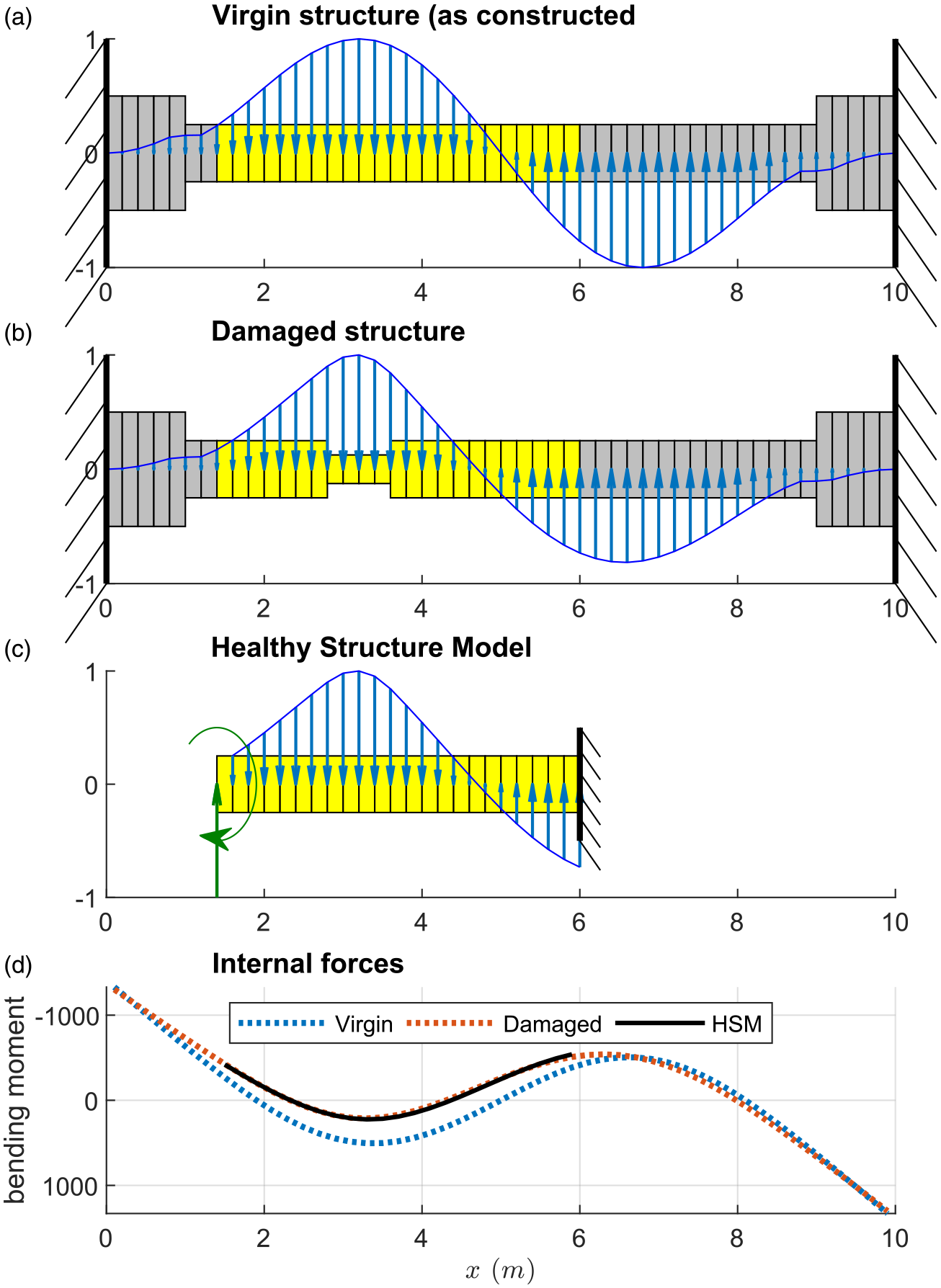
To better illustrate this concept, see Figure 2(a), where a virgin stepped and clamped-clamped beam is statically and uniformly loaded. When the structure is damaged (stiffness in some elements is decreased as shown in Figure 2(b)), the bending moment decreases and skews in the ROI (blue and red curves in Figure 2(d)) because the virgin and damaged structures are statically indeterminate, and the damage is asymmetrical.

Figure 2.

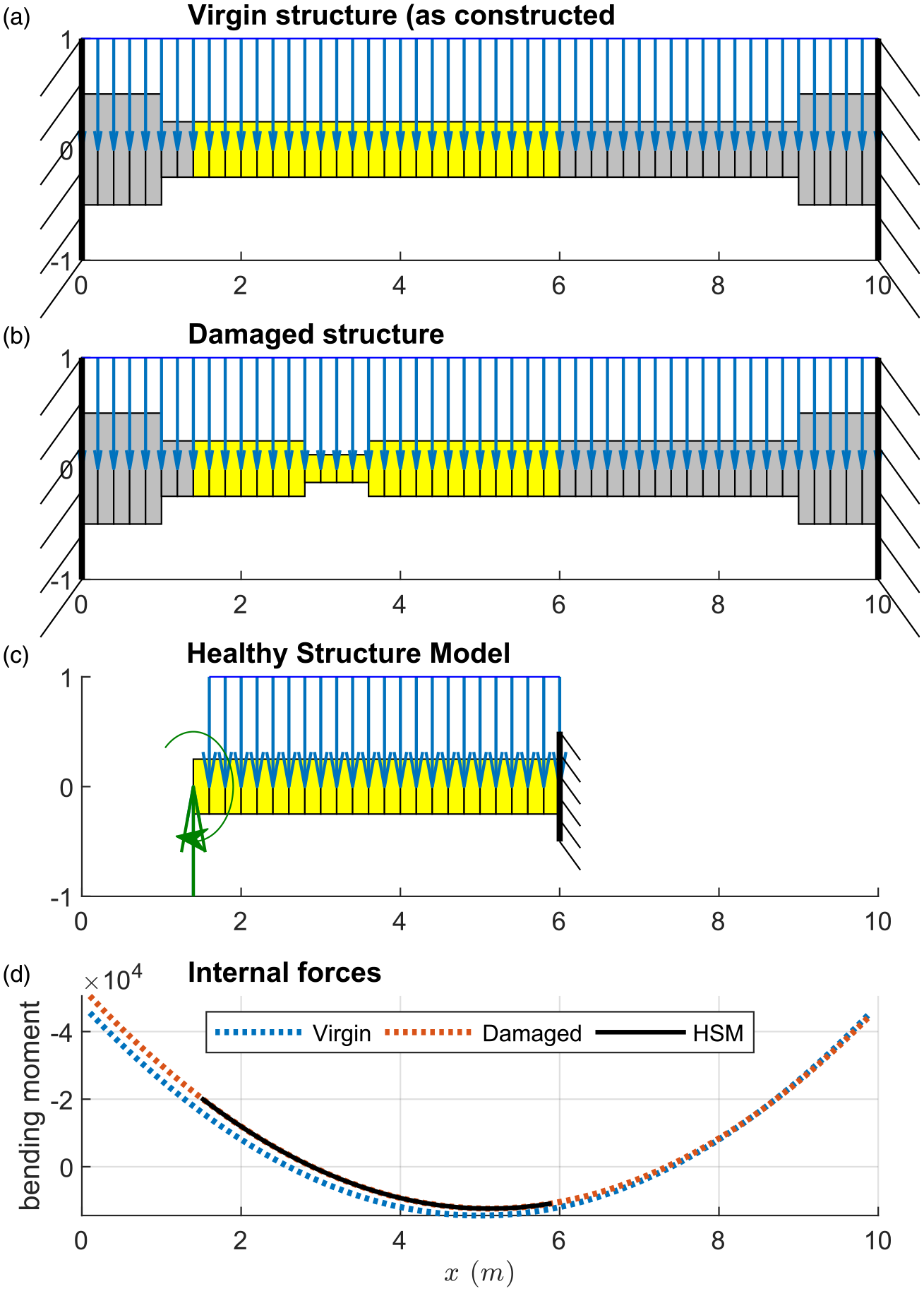
Illustrative example of a damaged structure with static load that has the same bending moment as a healthy-structure model (HSM) in the ROI (highlighted in yellow). This was generated using Euler–Bernoulli Finite Elements formulation.²¹

However, the new bending moment is still a quadratic function (a constant integrated twice). Therefore, a HSM can be conceived with exactly the same bending moment in the ROI (black curve in Figure 2(d)), given that the same load and some new and appropriate boundary conditions are applied to it.

As shown in Figure 2(c), a possible, but not unique, HSM consists in the ROI clamped in one end, and Neumann boundary conditions applied to the other: moment and force equal to the integration constants (green arrows). The bending moment corresponding to the HSM is, due to the uniformity of the load, a quadratic function (black curve). The HSM is not unique because other combinations of boundary conditions can also lead to the same bending moment; although with different displacements and rotations, which are not relevant to the purpose of the present work.

For the dynamic case, free vibrations in each vibration mode can be seen as a static load problem where the load is purely inertial and follows the displacement mode shape, weighted with the mass distribution. This is because displacements are proportional to accelerations when a single frequency is present, which is valid for each vibration mode.

In such a dynamic case, the equivalent static load shape can change considerably after damage, particularly in statically indeterminate structures. However, the shape of this new load distribution follows the weighted mode shape of the damaged structure. Therefore, the internal force can be calculated by successive integration of it. Then, the same reasoning made for the static case applies to the dynamic case of free vibrations. That is, the assumption of equation (3) holds exactly.

To better illustrate this concept, see Figure 3(a), where the previous virgin stepped and clamped-clamped beam is now loaded with a distribution following its 2nd mode shape weighted with its mass distribution. The resulting static displacements (not shown) are proportional to those of the mode shape (by definition of vibration mode), hence the equivalence. When the structure is damaged (stiffness in some elements is decreased, as shown in Figure 3(b)), the static-equivalent load changes, as the mode shape does, particularly in the damaged zone.

Figure 3.

Illustrative example of a damaged structure with inertial load produced during free vibrations that has the same bending moment as a healthy-structure model (HSM) in the ROI (highlighted in yellow). This was generated using Euler–Bernoulli Finite Elements formulation and lumped mass matrix.²¹

Also, the bending moment decreases and skews (blue and red curves in Figure 3(d)) because of three reasons: the virgin and damaged structures are statically indeterminate, the load changes, and the damage is asymmetrical. As the load is not uniform, the bending moment is not a quadratic function, but it is in both, in the damaged structure and in the HSM, the result of twice integrating the weighted mode shape of the damaged structure with appropriate integration constants (black curve in Figure 3(d)). These integration constants can be interpreted as new boundary conditions applied to the HSM, as shown in Figure 3(c).

If the Newmann boundary conditions (green arrows in Figure 3(c)) are equal to the integration constants, and the load is equal to that of the damaged structure, the bending moment in the HSM (black curve in Figure 3(d)) is equal to that of the damaged structure (red curve in Figure 3(d)) in the ROI. Again, the HSM that has the same bending moment as the damaged structure is not unique in general.

Sparsity of damage

Although it is not a general feature of every damaged structure, there are many cases in which the damage is confined in a small interval of the ROI. The sparsity of damage is due to at least two physical reasons. Sometimes, parts of structures are designed with uniform strength while the internal deformations are not (inefficient designs). Therefore, small zones with low safety factors usually appear. On the other hand, fragility of some structures makes that damage increases preferably where damage is already present. Sparsity of damage is related to the material used. For example, steel members can present fatigue cracks, which is a very concentrated type of damage. In case of reinforced concrete, which usually shows a crack band, the damage can be assumed as sparse only if the ROI is much longer than that band.

There is no consensus for a formal definition of sparsity. For the purpose of this work, sparsity is defined by using the measure of a set, denoted by the operator μ which assigns a number to each set. Here, the measure is simply the number of elements in the set if it is finite and countable (e.g. as in discrete sensing), or it is its length if it is a union of intervals (as in Continuum Mechanics).

Then, the assumption of damage sparsity (in the ROI) can be written as follows

k_{i} (x) = k_{ih} (x), x \in D_{h} \subset D_{ROI},

(4)

such that μ(D_h) > 0.5μ(D_ROI). The coefficient 0.5 is just a theoretical threshold indicating the majority. In practice, it is preferable that μ(D_h) >> 0.5μ(D_ROI).

Next, an important and useful consequence of the sparsity of damage is shown. From the combination of equations (1), (3) and (4), it follows that

d_{i} (x) = d_{ih} (x), x \in D_{h} \subset D_{ROI} .

(5)

In simple words, if the internal force is assumed to be invariant to damage (damaged structure compared to the HSM), the sparsity of damage implies the sparsity of the fluctuations (due to damage) in the internal deformations.

Proposal

Now, the proposal to estimate $H_{k_{i}} (x)$ can be stated simply. Instead of using the internal forces and deformations for updating the stiffnesses of the healthy and damaged structures (as usual in model updating), this simple equation can be used

H_{k_{i}} (x) = \frac{d_{ih} (x)}{d_{i} (x)}, x \in D_{ROI} .

(6)

which follows from equations (2) and (3). The internal deformations d_i(x) can be obtained from measurements of the damaged structure and d_ih(x) is the HSMR, which can be synthesised as described below.

The differential equation of the HSM can be written in general as

d_{ih}^{'} (x) = g (d_{ih} (x), p_{0}^{*}, q (x)), x \in D_{ROI},

(7)

where d _ih(x) is a vector function containing the n_ep state variables at x (d_ih(x) and its n_ep− 1 successive derivatives), $p_{0}^{*}$ is a vector containing the n_ip internal parameters and q(x) is the loading model. Note that q(x) does not define completely the load but it is a function representing its distribution. Load parameters (e.g. magnitude) are also contained in $p_{0}^{*}$ for convenience.

The load shape is considered as known and the load magnitude as unknown due to practical reasons. In a static load situation, it is usually easy to determine the load shape by inspection of the geometry; however, knowing its magnitude requires an additional measurement campaign. A trivial example is the case of a prismatic beam, whose precise cross-section is unknown, loaded with its self-weight. In free vibrations, the inertial load produced by each vibration mode can be treated as a static load whose magnitude is indeterminate but its shape follows the vibration mode shape weighted by the mass distribution shape. A trivial example is the case of a uniform beam or bar; in that case, the equivalent static load shape is equal to the vibration mode shape.

The solution of this differential equation is

d_{ih} (x) = g (p^{*}, q (x)), x \in D_{ROI},

(8)

where p * contains the n_ip + n_ep internal and external parameters. For many simple problems (e.g. bars or beams), an analytical solution for g(x) can be easily found.

The only remaining task for synthesising the HSMR is to find the values of the parameters contained in p *. To do that, this work proposes using the sparsity consequence stated in equation (5) and some robust regression technique to find d_ih(x) from d_i(x). In this work, that problem is stated as

p^{*} = \arg \min_{\begin{matrix} p \\ x \in D_{ROI} \end{matrix}} ‖ d_{i} (x) - g (p, q (x)) ‖ 1,

(9)

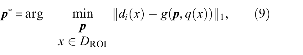
where ‖•‖₁, that is, the 1-norm, has been used just for simplicity. Equation (9) is the search for the values of p that minimise the sum or the integral of the absolute deviations between d_i(x) and d_ih(x). This (or another) robust regression technique rejects outliers, which hopefully are the points outside D_h. Note that the parameters determining the HSMR (d_ih) could be fitted using only the deformations of the damaged structure (d_i); because such deformations are the same inside D_h, and the points outside D_h are rejected by the robust property of the regression technique.

The particular case of the 1-norm can be thought of as a weighted least-squares fitting where weights are inversely proportional to the absolute deviations. Therefore, points with large deviation are ‘rejected’. In order to guarantee uniqueness of the solution, this problem is solved by using the solution of the equivalent least square problem as a starting point.

On the other hand, since equation (5) holds with the parameters found, and equation (4) is assumed, the internal force of the damaged structure (f_i(x)) in the ROI is the same as that corresponding to the synthesised HSMR (f_ih(x)), at least in D_h. Besides, since (1) f_i(x) and f_ih(x) are the solutions of successive integration of the same load and (2) D_h covers most of the ROI, the integration constants and load magnitude are also the same for the damaged and healthy model structures. Therefore, equation (3) holds also in the whole ROI. A more detailed analysis of the internal force invariability is made in each of the following two application examples.

Now that the HSMR has been synthesised, it is ready to be used as reference in a damage identification method based on equation (6), without needing actual measurements of the healthy structure. Besides, the HSM is not required in practice, the HSMR is enough to (detect, locate and) quantify damage.

Application examples

In this section, the general formulation is specialised for four particular cases: bar and beam, each with static or dynamic response.

Bar under normal force

For the case of a bar that is uniform in the ROI, with unknown internal stiffness EA_h, loaded with distributed axial force³ with unknown amplitude Q and known shape q(x), and choosing $d_{ih} (x) = u_{x}^{'} (x)$ , equation (7) reduces to

d_{ih}^{'} (x) = p_{1}^{*} q (x), x \in D_{ROI} = [x_{i}, x_{f}],

(10)

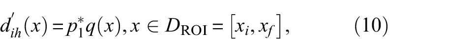
where $p_{1}^{*} = \frac{Q}{E A_{h}}$ is the only internal parameter.

The solution of this differential equation is

d_{ih} (x) = p_{1}^{*} \int_{x_{i}}^{x} q (χ) d χ + p_{2}^{*}, x \in D_{ROI},

(11)

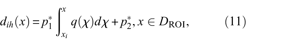
where $p^{*} = {[p_{1}^{*} p_{2}^{*}]}^{⊤}$ contains the internal and external parameters.

Note that an advantage of stating the differential equation in terms of deformation, instead of displacements, is that the number of integration constants is reduced to 1.

Now, if d_i(x) is known⁴ at x₁, x₂, …, x_N points (with N preferably much larger than 2), the unknown parameters can be found by solving the following problem

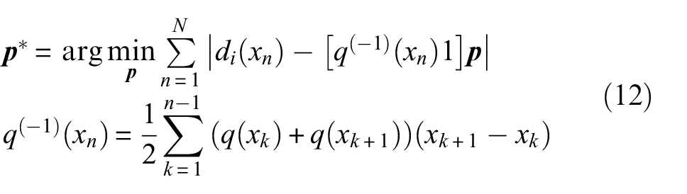
\begin{matrix} p^{*} = \arg min_{p} \sum_{n = 1}^{N} | d_{i} (x_{n}) - [q^{(- 1)} (x_{n}) 1] p | \\ q^{(- 1)} (x_{n}) = \frac{1}{2} \sum_{k = 1}^{n - 1} (q (x_{k}) + q (x_{k + 1})) (x_{k + 1} - x_{k}) \end{matrix}

(12)

where $p = {[p_{1} p_{2}]}^{⊤}$ , and trapezoidal integration has been used for simplicity, but other suitable technique could have been chosen instead. At any rate, this statement relies on the sparsity consequence of equation (5).

Regarding the internal force invariability, the following analysis can be made. If d_i(x) = d_ih(x) in at least 2 points x₁, x₂ of D_h (where it was assumed that k_i(x) = k_ih(x)), then f_i(x) = f_ih(x) in those points. Besides, both internal forces are entirely determined by only two parameters, that is

\begin{matrix} f_{i} (x) & = Qr (x) + C, x \in D_{ROI}, \end{matrix}

(13)

\begin{matrix} f_{ih} (x) & = Q_{h} r (x) + C_{h}, x \in D_{ROI} \end{matrix}

(14)

r (x) = \int_{x_{i}}^{x} q (χ) d χ

(15)

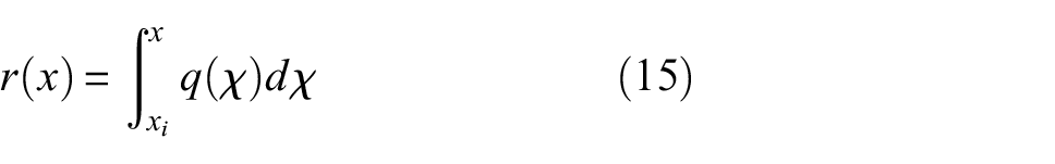
Therefore, if r(x₁) ≠r(x₂), internal forces are the same in the whole ROI because the solution of the resulting system of equations is Q = Q_h, C = C_h, that is, Equation (3) holds exactly. The more points D_h has, the more likely is to find x₁, x₂ such that r(x₁) ≠r(x₂).

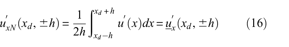
In practice, d_i(x_d) is not measured directly but estimated from measurements of u_x(x_d) and numerical differentiation, which produce

u'_{x N} (x_{d}, \pm h) = \frac{u_{x} (x_{d} + h) - u_{x} (x_{d} - h)}{2 h} \approx u'_{x} (x_{d}) = d_{i} (x_{d})

where central difference has been used and sensors separation is 2h (since u_x(x_d) has a weight equal to 0 in the formula). The difference between $u_{x}^{'} (x_{d})$ and $u_{xN}^{'} (x_{d}, \pm h)$ is due to the precision and truncation errors. Neglecting the first one, and using the Fundamental Theorem of Calculus, it can be shown that

u_{xN}^{'} (x_{d}, \pm h) = \frac{1}{2 h} \int_{x_{d} - h}^{x_{d} + h} u^{'} (x) dx = {\underline{u}}_{x}^{'} (x_{d}, \pm h)

(16)

where ${\underline{u}}_{x}^{'} (x_{d}, \pm h)$ is the mean value of the derivative of u_x in the interval [x_d−h, x_d + h].

This important fact and the application of a procedure similar to the one described in ref. 19 lead to a more accurate interpretation of equation (2) when the quotient of numerical derivatives are used: The calculated indicator is the reduction in the mean stiffness, which unfortunately depends on the sensor separation h, and therefore, it is not a direct quantifier of damage. That is

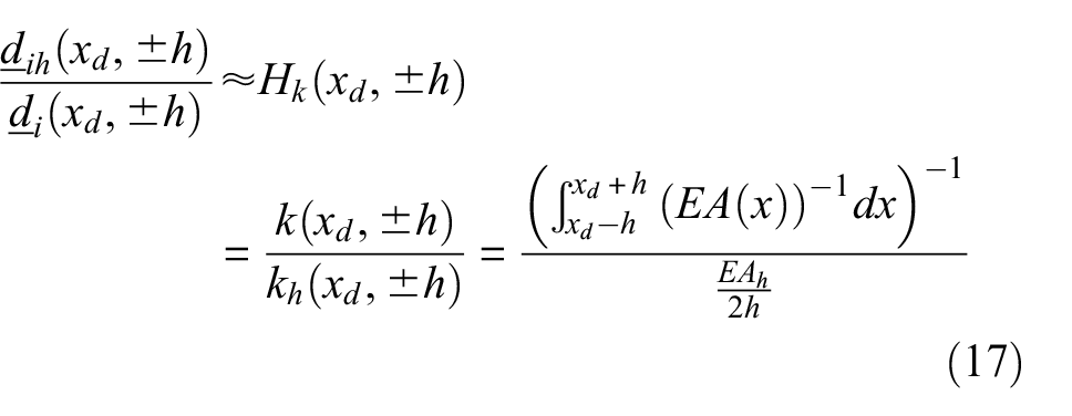
\begin{matrix} \frac{{\underline{d}}_{i h} (x_{d}, \pm h)}{{\underline{d}}_{i} (x_{d}, \pm h)} \approx H_{k} (x_{d}, \pm h) \\ = \frac{k (x_{d}, \pm h)}{k_{h} (x_{d}, \pm h)} = \frac{{(\int_{x_{d} - h}^{x_{d} + h} {(E A (x))}^{- 1} d x)}^{- 1}}{\frac{E A_{h}}{2 h}} \end{matrix}

(17)

where it has been assumed that d_i(x) does not change sign in the interval [x_d−h, x_d + h] for applying the Weighted Mean Value Theorem.

In order to find a direct quantifier of damage, it is assumed a bi-linear variation for EA(x) around the location of the actual damage. Thus, the following relation can be found⁵

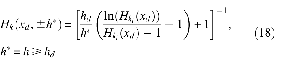
\begin{matrix} H_{k} (x_{d}, \pm h^{*}) = {[\frac{h_{d}}{h^{*}} (\frac{\ln (H_{k_{i}} (x_{d}))}{H_{k_{i}} (x_{d}) - 1} - 1) + 1]}^{- 1}, \\ h^{*} = h \geq h_{d} \end{matrix}

(18)

which allows calculating $H_{k_{i}} (x_{d}) = H_{EA} (x_{d})$ , an indicator that quantifies the damage independently of the sensor separation, from H_k(x_d, ±h*). Here, 2h_d is the damage apparent extent, which is related to Saint Venant’s principle, as discussed in ref. 19; and 2h* is the length of the interval in which the derivative is implicitly averaged by the numerical differentiation formula.

Beam under bending moment

For the case of a beam that is uniform in the ROI, with unknown internal stiffness EI_h, loaded with a distributed transverse force having unknown amplitude Q and known shape q(x), and choosing $d_{ih} (x) = u_{y}^{''} (x)$ , equation (7) reduces to

d_{ih}^{''} (x) = p_{1}^{*} q (x), x \in D_{ROI} = [x_{i}, x_{f}],

(19)

where $p_{1}^{*} = Q / Q E I_{h} E I_{h}$ is the only internal parameter.

The solution of this differential equation is

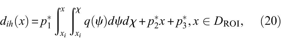
d_{ih} (x) = p_{1}^{*} \int_{x_{i}}^{x} \int_{x_{i}}^{χ} q (ψ) d ψ d χ + p_{2}^{*} x + p_{3}^{*}, x \in D_{ROI},

(20)

where $p^{*} = {[p_{1}^{*} p_{2}^{*} p_{3}^{*}]}^{⊤}$ contains the internal and external parameters.

Note that the number of integration constants is reduced to 2 (the state variables are d_ih(x) and $d_{ih}^{'} (x)$ ).

Now, if d_i(x) is known⁶ at x₁, x₂, …, x_N points (with N preferably much larger than 3), the unknown parameters can be found by solving the following problem

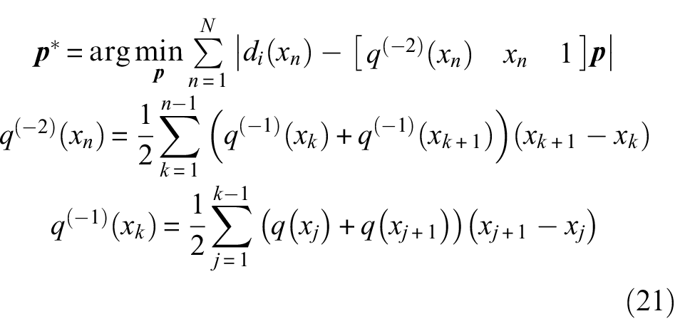
\begin{matrix} p^{*} = \arg min_{p} \sum_{n = 1}^{N} | d_{i} (x_{n}) - [\begin{matrix} q^{(- 2)} (x_{n}) & x_{n} & 1 \end{matrix}] p | \\ q^{(- 2)} (x_{n}) = \frac{1}{2} \sum_{k = 1}^{n - 1} (q^{(- 1)} (x_{k}) + q^{(- 1)} (x_{k + 1})) (x_{k + 1} - x_{k}) \\ q^{(- 1)} (x_{k}) = \frac{1}{2} \sum_{j = 1}^{k - 1} (q (x_{j}) + q (x_{j + 1})) (x_{j + 1} - x_{j}) \end{matrix}

(21)

where $p = {[p_{1} p_{2} p_{3}]}^{⊤}$ , and trapezoidal integration has been used twice. The statement of this optimisation problem is also based on the sparsity consequence of equation (5).

Regarding the internal force invariability, the following analysis can be made. Both internal forces are entirely determined by only three parameters, that is

f_{i} (x) = Qr (x) + C_{1} x + C_{2}, x \in D_{ROI},

(22)

f_{ih} (x) = Q_{h} r (x) + C_{h 1} x + C_{h 2}, x \in D_{ROI}

(23)

r (x) = \int_{x_{i}}^{x} \int_{x_{i}}^{χ} q (ψ) d ψ d χ

(24)

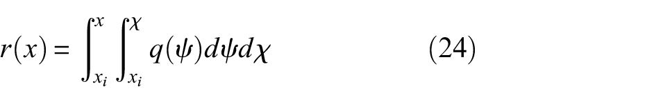
Besides, if d_i(x) = d_ih(x) in at least 3 points x₁, x₂, x₃ of D_h (where it was assumed that k_i(x) = k_ih(x)), then f_i(x) = f_ih(x) in those points, which leads to this homogeneous system of linear equations

Ab = 0_{3 \times 1}

(25)

\begin{matrix} A = [\begin{matrix} r (x_{1}) & x_{1} & 1 \\ r (x_{2}) & x_{2} & 1 \\ r (x_{3}) & x_{3} & 1 \end{matrix}], b = [\begin{matrix} Q - Q_{h} \\ C_{1} - C_{1 h} \\ C_{2} - C_{2 h} \end{matrix}] \end{matrix}

(26)

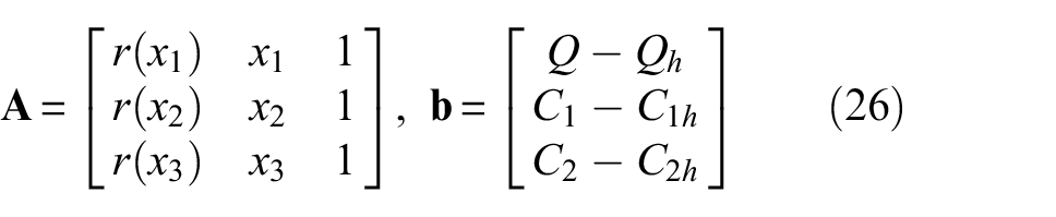
If det(A) ≠ 0, internal forces are the same in the whole ROI because the only solution of the resulting system of equations is b = 0_3×1. Therefore, equation (3) holds exactly. The more points D_h has, the more likely is that det(A) ≠ 0.

As in the case of a bar, in practice, the quotient of the numerical curvatures is usually calculated. Therefore, $H_{k_{i}} (x_{d}) = H_{EI} (x_{d})$ , an indicator that quantifies the damage independently of sensor separation h, must be obtained from H_k(x_d, ±h*) using the following relation

\begin{matrix} H_{k} (x_{d}, \pm h^{*}) = {[\frac{h_{d}}{h^{*}} (\frac{\ln (H_{k_{i}} (x_{d}))}{H_{k_{i}} (x_{d}) - 1} - 1) + 1]}^{- 1}, \\ h^{*} = \frac{h}{2} \geq h_{d} \end{matrix}

(27)

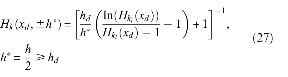
where 2h* is the length of the interval where the numerical second derivative implicitly averages the curvature. This relation is derived in section 2.3 of ref. 19. In that work, it was numerically and statistically shown that the apparent damage extent 2h_d of a single crack is strongly related to the beam cross-section height h_s, and it is almost independent on the crack depth, that is, h_d ≈ h_s/2.

Equation (27) also relies on the assumption that d_i(x) does not change sign in the interval [x_d−h*, x_d + h*] for applying the Weighted Mean Value Theorem (Appendix D in ref. 19).

Static response

If the bar or the beam is statically loaded, q(x) does not depend on d_i(x), but on external causes (e.g. weight). Assuming those are known, equations (12) or (21) can be used directly.

Since the assumption of equation (3) holds exactly, equation (6) can then be used to quantify damage without no other error than those produced by the measurements, the method used to find d_i(x) (e.g. numerical differentiation), and deviations from the analytical models.

To illustrate this static application in a beam, the example of Figure 2 is reconsidered. The curvatures resulting from a Finite Element analysis of the virgin and damaged structures, using 100 Euler–Bernoulli elements,²¹ are displayed as blue and red curves in Figure 4(a). When equation (21) is applied to the curvature of the damaged structure, equation (20) yields the black curve of Figure 4(a). It is clear that the HSMR is exactly equal to the curvature of the damaged structure (red curve in Figure 4(a)) in the healthy zones, while the curvature of the virgin structure (blue curve in Figure 4(a)) is only similar to it.

Figure 4.

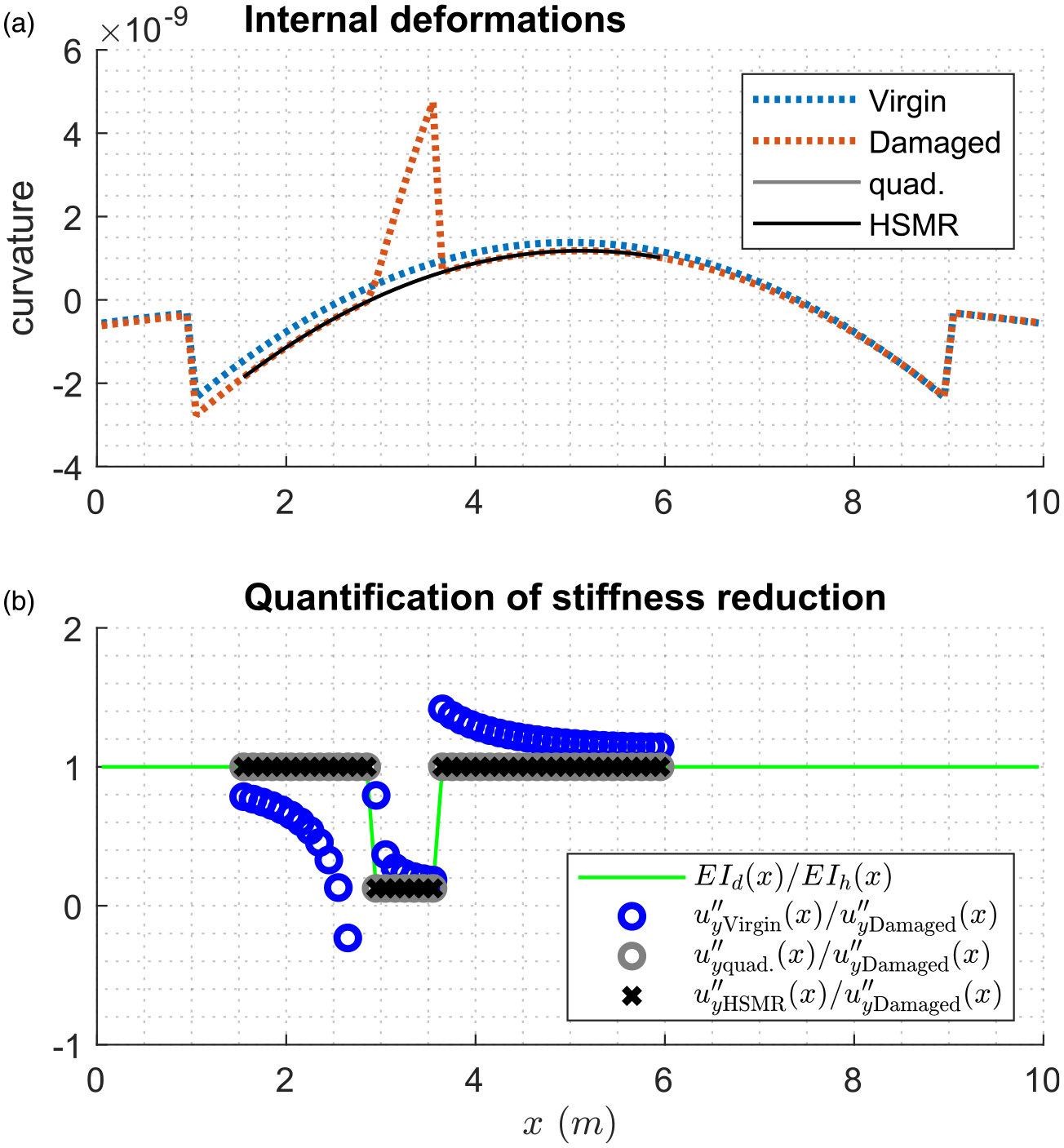
Curvatures of the virgin, damaged and healthy model structures of Figure 2 and their ratios compared to the actual stiffness reduction.

The apparently small difference between the curvatures of the virgin and damaged structures in the healthy zones is drastically amplified when they are used to estimate damage by means of a ratio. This is evident when comparing the green curve to the blue circles in Figure 4(b). When doing this, it can be seen that the quotient of curvatures is similar to the stiffness reduction in the damaged zone. However, the error in the healthy zones is huge (out of scale in some cases). From the point of view of the authors, there is an important teaching here: measurements of the virgin structure are not only hard to get, they can also be inconvenient.

On the other hand, using equation (6) with the synthesised HSMR, the damage quantification is exact (neglecting the numerical error of the Finite Element solver), as can be seen when comparing the black crosses to the green curve in Figure 4(b). Finally, as another benchmark, a quadratic robust fit was used to generate an alternative HSMR (grey curve in Figure 4(a)), which in this case of uniform load, has the same performance (grey circles in Figure 4(b)) than the method proposed in this paper (black crosses in Figure 4(b)).

Dynamic response

If the bar or the beam is dynamically loaded, there are some possibilities to adapt equations (12) or (21). The simplest is to work with the free vibrations (found, e.g. automatically by an algorithm as in ref. 22). In free vibrations, q(x) is an inertial load proportional to the mass distribution and accelerations. If a vibration mode is considered separately, the load is also proportional to the (weighted) displacements u(x) = u_x(x) (bar) or u(x) = u_y(x) (beam) of the vibration mode.

If mode shape displacements, velocities or accelerations are measured, the internal deformation d_i(x) is found by differentiating the corresponding displacements u(x), and equations (12) or (21) can be used by just substituting

q (x) = u (x) m (x),

(28)

where u(x) is some vibration mode shape, and m(x) is the shape in which mass is distributed along the bar or beam. Note that the actual mass scaling and the natural frequency are absorbed into the parameter p₁ in equations (12) (bar) or (21) (beam).

On the other hand, if the internal deformations are measured directly (e.g. using strain gauges), q(x) can be found by integration. In this case, one or two new integration constants appear, which are simply additional internal parameters: p₃ (bar), or p₄ and p₅ (beam).

To illustrate this dynamic application in a beam, the example of Figure 3 is also reconsidered. The curvatures of the virgin and damaged structures were calculated through Finite Element Analyses, using 100 Euler–Bernoulli elements,²¹ and they are displayed as blue and red curves in Figure 5(a). When equation (21) is applied to the curvatures of the damaged structure, equation (20) yields the black curve of Figure 5(a). It is clear that this synthesised HSMR is exactly equal to the curvature of the damaged structure (red curve in Figure 5(a)) in the healthy zones; neglecting the numerical errors of the Finite Element solver and trapezoidal integration method. For its part, the curvature of the virgin structure (blue curve in Figure 5(a)) is only similar to the curvature of the damaged structure (red curve in Figure 5(a)) in the healthy zones.

Figure 5.

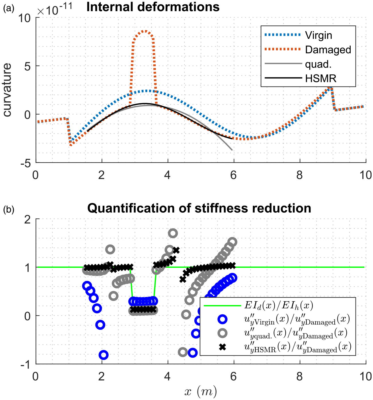
Curvatures of the virgin, damaged and healthy model structures of Figure 3, and their ratios compared to the actual stiffness reduction.

In this case of non-uniform load, the benchmark quadratic robust fit (grey curve in Figure 5(a)) has a performance evidently poorer than that of the method proposed in this paper (black curve in Figure 5(a)), mainly because the ROI in the HSM encompasses significant change of curvature that the quadratic function is unable to capture. However, in the healthy zones, the grey curve is still more similar to the curvature of the damaged structure (red curve in Figure 5(a)) than the curvature of the virgin structure (blue curve in Figure 5(a)).

Again, the difference between the curvatures of the virgin and damaged structures in the healthy zones is drastically amplified when they are used to estimate damage by means of a ratio. This is evident when comparing the green curve to the blue circles in Figure 5 (b). When doing this, it can be seen that the quotient of curvatures is similar to the stiffness reduction in the damaged zone. However, the error in the healthy zones is huge (several points are out of scale).

In this case, in which the mode shape contains inflexion points in the ROI, the curvatures cross zero (x = 2.25 m, x = 4.5 m), which amplifies even more the small differences between the curvatures when ratios are calculated in the healthy zones. This is simply because propagation error in quotients is inversely proportional to the absolute values of the numerator and denominator.²³ Therefore, near those zero crossings, the three methods here compared present significant error. As in ref. 20, ‘there is no risk of confusing these spikes with damage because we can always check to see if the curvature is zero, or less than a specified tolerance at any such spike’. In ref. 20, they considered the calculated second derivative to be zero if it is less than 10⁻⁷ in absolute value, which is appropriate for numerical simulations. In a practical application, that tolerance should set depending on the precision, noise and spacing of the sensors and on the numerical differentiation method.

At any rate, using the synthesised HSMR has clearly the best performance (black crosses in Figure 5(b)), and even the quadratic robust fit (grey circles in Figure 5(b)) has better performance than using the curvatures of the virgin structure (blue circles in Figure 5(b)). The latter makes the importance of collecting virgin state measurements questionable, especially in statically indeterminate structures, where a local damage induces global changes in the internal force. Note also that, if the virgin structure had had manufacturing defects, the difference in the performance of the methods would have been even greater.

Comparison with two benchmark methods

In order to contrast the proposed method with a similar technique that has been widely cited, that is, the Gapped Smoothing Method (GSM),¹⁵ and with its extension, that is, the Global Fitting Method (GFM),¹⁶ the example of Figures 3 and 5, is reconsidered once again. This time, two simultaneous flaws of different characteristics are present in the damaged beam: the original zone of constant reduced stiffness (2.9 m ≤x≤ 3.6 m) and a zone of variable stiffness (2 m ≤x≤ 2.6 m). This damage scenario enables a more robust comparison.

The following is a description of the core formulation of each benchmark method. Further statistical and/or multi-modal post-processing has been omitted to compare methods of similar complexity and using the same input data.

The GSM consists in fitting, exactly, a cubic polynomial to the 2 points before and the 2 points after the current point of the mode shape curvature of the damaged beam, that is

P_{3 i} (x) = a_{0} + a_{1} x + a_{2} x^{2} + a_{3} x^{3},

(29)

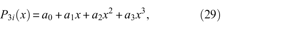
with coefficients a₀, a₁, a₂, a₃ such that

P_{3 i} (x_{k}) = u_{y}^{''} (x_{k}), for k = i - 2, i - 1, i + 1, i + 2 .

(30)

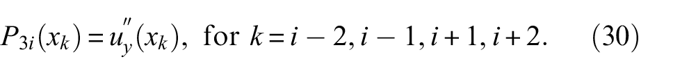
Then, a damage index is calculated at each point as¹⁵

D_{GSM} (x_{i}) = P_{3 i} (x_{i}) - u_{y}^{''} (x_{i})

(31)

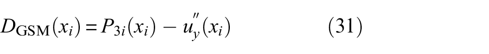
For ease of comparison, a health index is here defined as

H_{GSM} (x_{i}) = 1 - \frac{D_{GSM} (x_{i})}{max (| D_{GSM} |)}

(32)

On the other hand, the GFM consists in fitting, in a least-squares sense, the generic form of the mode shape of a healthy beam to all the points (in a ROI) of the mode shape of the damaged beam, that is

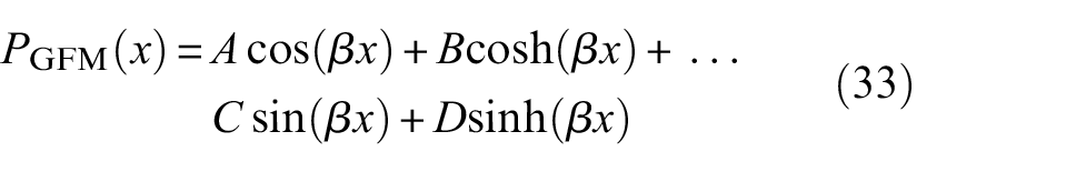
\begin{matrix} P_{GFM} (x) = & A \cos (β x) + B \cosh (β x) + \dots \\ C \sin (β x) + D \sinh (β x) \end{matrix}

(33)

with coefficients A, B, C, D, β such that

min ‖ P_{GFM} (x) - u_{y} (x) ‖ 2

(34)

Then, a damage index is calculated at each point as¹⁶

D_{GFM} (x_{i}) = | u_{y}^{''} (x_{i}) - P_{GFM}^{''} (x_{i}) |

(35)

For ease of comparison, the following health index is defined here

H_{GFM} (x_{i}) = 1 - \frac{D_{GFM} (x_{i})}{max (| D_{GFM} |)}

(36)

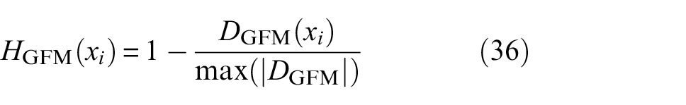
Figure 6(a) and (b) displays the displacement and curvature of the first mode shape of the damaged beam, while Figure 6(c) shows the result of applying equations (32) and (36), and the proposed method to that input data.

Figure 6.

Comparison of the proposed method to the Gapped Smoothing Method (GSM),¹⁵ and its successor, that is, the Global Fitting Method (GFM)¹⁶; using the first mode shape of a damaged beam.

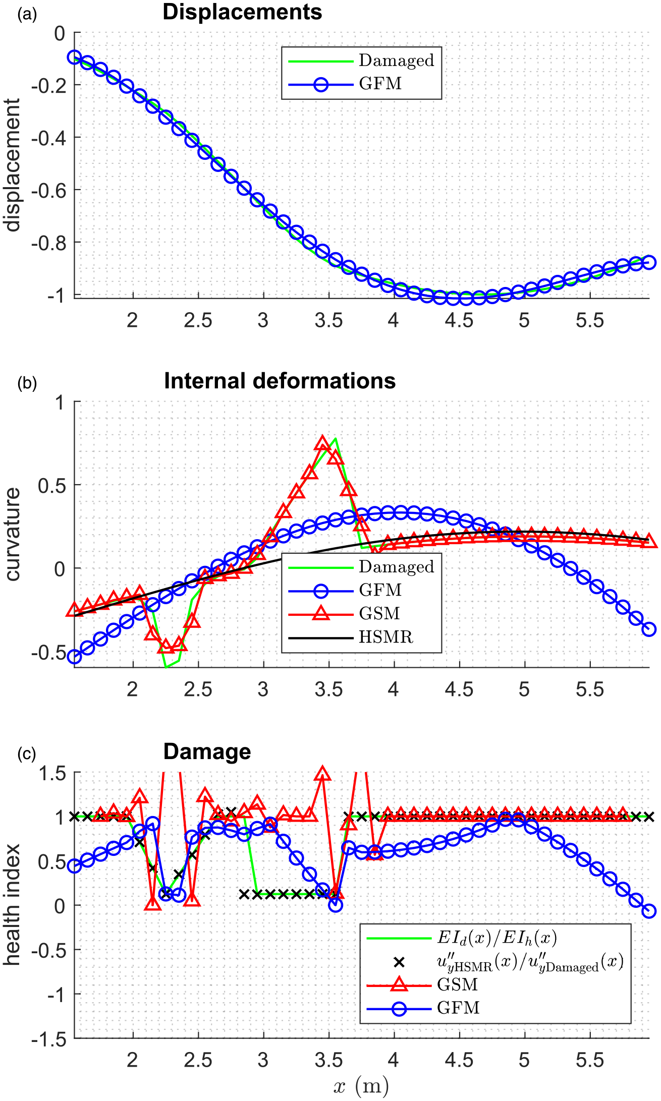
As regards to the GSM, Figure 6(b) shows the result of equation (29) in red. There, it can be seen that the generated curvature exactly fits the damaged beam curvature in the healthy zones. When inspecting the red curve in Figure 6(c), it becomes evident that the GSM is sensitive to changes in stiffness but only in a local sense. Therefore, it presents false negatives inside the damaged zone with constant stiffness (3.1 m ≤x≤ 3.4 m). A clear advantage of the GSM is its immunity to false positives around inflexion points, which is because the index is defined as a difference and not as a ratio. However, if the two main spikes in this red curve are used as indicators of the damaged zone ends (as suggested in ref. 12 for plates), it could be interpreted (depending on the threshold) that such a zone goes from 2.5 m to 3.4 m, which would imply a false positive at x = 2.7 m.

Regarding the GFM, Figure 6(a) shows the result of equation (33) in blue. There, it can be seen that the generated displacement globally fits the damaged beam displacement. The corresponding curvature, shown in blue in Figure 6(b), also fits the damaged beam curvature in a global sense. Therefore, it does not exactly fit the curvature in the healthy zones (as the GSM does). The consequence is that the GFM outcomes false positives, for example, where x≥ 5.5 m in Figure 6(c). The advantage of the GFM over the GSM is that the GFM avoids false negatives in the damaged zone with constant stiffness (3.1 m ≤x≤ 3.4 m).

Clearly, the GSM and the GFM are level 2 damage identification methods. On the contrary, the proposed method also allows quantifying damage (level 3) without further post-processing. This is evident in the damaged zone of variable stiffness (see Figure 6(c) in 2 m ≤x≤ 2.6 m), where the proposed method exactly estimates the stiffness reduction. The only failure of the proposed method in this case occurs at the inflexion point (x = 2.85 m), which is a false positive. Interestingly, the proposed method is unlikely to outcome false negatives, because that would require a small curvature in a zone of reduced stiffness (which naturally tends to have a large curvature).

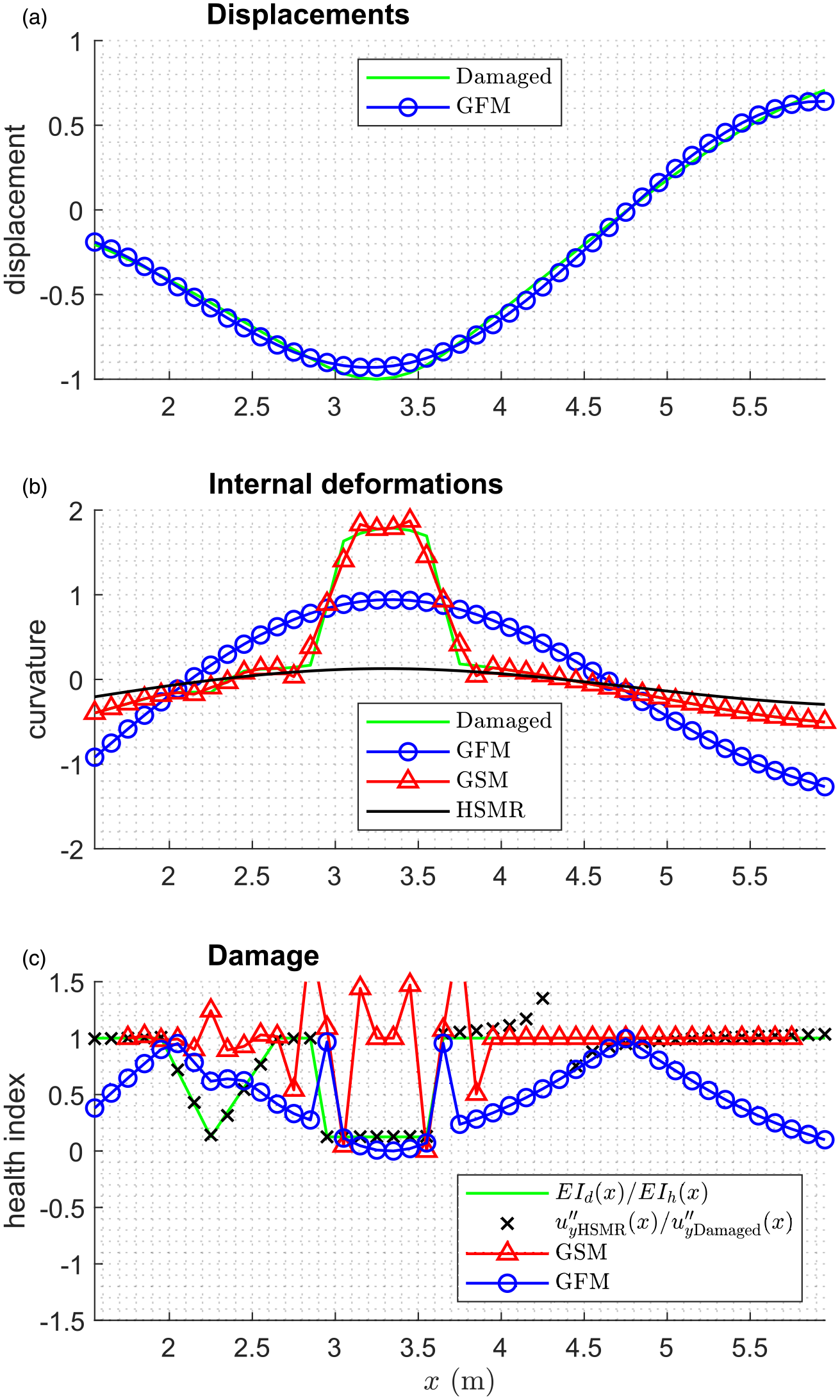
Figure 7 shows the same sort of results as Figure 6 for the shape of the second mode. The performance of the GSM is not significantly affected by the change of the mode order. On the contrary, as can be seen in 7(c) for 2.6 m ≤x≤ 2.9 m, the false positive performance of the GFM is even worse, probably because the wave length is more similar to the damaged zones extent. The proposed method, on the other hand, displays almost the same performance, except for the fact that an additional inflexion point occurs in the ROI, which outcomes a false positive at x = 4.4 m.

Figure 7.

Comparison of the proposed method to the Gapped Smoothing Method (GSM),¹⁵ and its successor, that is, the Global Fitting Method (GFM)¹⁶; using the second mode shape of a damaged beam.

Demonstration examples

In the examples analysed so far, the proposal of synthesising a HSMR shows excellent performance for detecting, locating and quantifying damage because of four reasons: (1) the beams were modelled using Euler–Bernoulli elements and a lumped mass matrix; (2) the measurement error was not simulated (although its effect can be anticipated from what was seen with the numerical error); (3) damage was simulated as flexural rigidity reduction, instead of modelling an actual crack in detail; and (4) measurements were assumed to be available at each single node, so equation (27) was not involved, and exact curvature was available at each element by difference of node rotations. These ideal conditions were considered just to highlight the inherent characteristics of the proposed method. The following demonstration examples consider more realistic situations.

Numerical example using dynamic response

In order to demonstrate the proposal in a concrete example with nontrivial boundary conditions and not assuming an Euler–Bernoulli model, the rubber-supported three-span bent steel beam that is shown in Figure 8 was numerically modelled using elastic solid elements through the Finite Element (FE) method.

Figure 8.

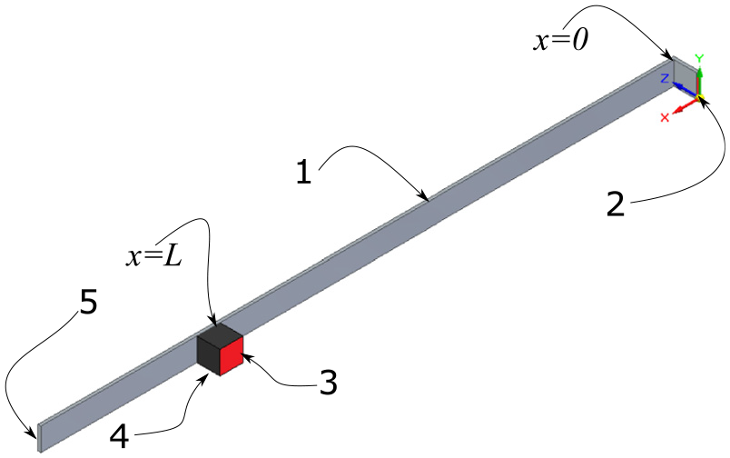
Beam modelled numerically with dynamic response. References: 1. first span of the steel beam; 2. fixed support at the first end; 3. fixed support at the base of the rubber block; 4. rubber block and 5. free end.

The beam is made of a 0.7254 m long steel flat strip that is bent and fixed at one end and free at the other. The cross-section is 0.0254 m wide and 0.003175 m high. At x = L = 0.5 m, it is supported on a 0.0254 m cubic rubber block. This example was selected for its nontrivial boundary conditions.

Regarding the material properties, the steel flat strip has an elastic modulus of E = 210 GPa, a mass density of ρ = 7850 kg/m³ and a Poisson’s ratio of ν = 0.3. The material properties of the rubber block are: E = 1 MPa, ρ = 1000 kg/m³ and ν = 0.48.

The FE model was created using ANSYS-APDL.²⁴ All the elements were 8-node SOLID185 of the same size, and 8 of them were placed along the cross-section height. Thus, the steel beam reaches a total of 935823 elements while the rubber block has 262144.

Cracks were modelled by avoiding node connectivity between two consecutive elements along the cross-section width and along the crack depth at the crack location. This type of isolated crack can occur in metallic structures because of fatigue failures or welding flaws.

The solution of a modal analysis for the first mode shape displacements was used as input to the damage quantification method here proposed. Measurement error was simulated by rounding these analysis results to 4 significant digits. Displacements curvatures d_i(x) were estimated by using the central difference numerical derivative formula, and d_ih(x) was synthesised using equation (21).

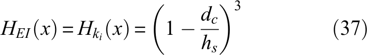
The series of 6 cases shown in Table 1 was considered. These cases include up to 2 rectangular Mode I cracks, one at the mid-span and other at 3/4 of the span length. Since the cross-section is rectangular, the actual value of the damage indicator can be estimated by geometry simply as

H_{EI} (x) = H_{k_{i}} (x) = {(1 - \frac{d_{c}}{h_{s}})}^{3}

(37)

Table 1.

Crack depth d_c (and actual value of $H_{k_{i}} (x_{d})$ ) of the cases considered for the beam with dynamic response.

Case	x _d = L/2 = 0.25 m	x _d = 3L/4 = 0.375 m
Case 0	0 (1.00)	0 (1.00)
Case 1	h _s/4 (0.42)	h _s/8 (0.67)
Case 2	h _s/8 (0.67)	h _s/4 (0.42)
Case 3	h _s/8 (0.67)	h _s/8 (0.67)
Case 4	h _s/4 (0.42)	0 (1.00)
Case 5	h _s/2 (0.13)	0 (1.00)

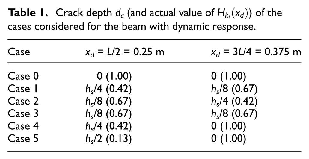
where d_c is the crack depth; h_s is the cross-section height and two assumptions have been made: the reduction in stiffness is only due to the reduction in the moment of inertia of the cross-section and the neutral axis is at the middle of the remaining cross-section height.

The sensors were assumed to be equally spaced with h = 0.025 m, which in practice can be achieved by using a scanning laser vibrometer. Since the number of data points can be very influential in the performance of the method, three different ROI sizes were considered: (1) D_ROI = [0.05 m, 0.45 m] (μ(D_ROI) = 17), (2) D_ROI = [0.2 m, 0.425 m] (μ(D_ROI) = 10) and (3) D_ROI = [0.25 m, 0.375 m] (μ(D_ROI) = 6).

Figure 9, Figure 10, and Figure 11 show the results of the method using those three ROIs for the six cases, in comparison with the previously calculated actual damage. 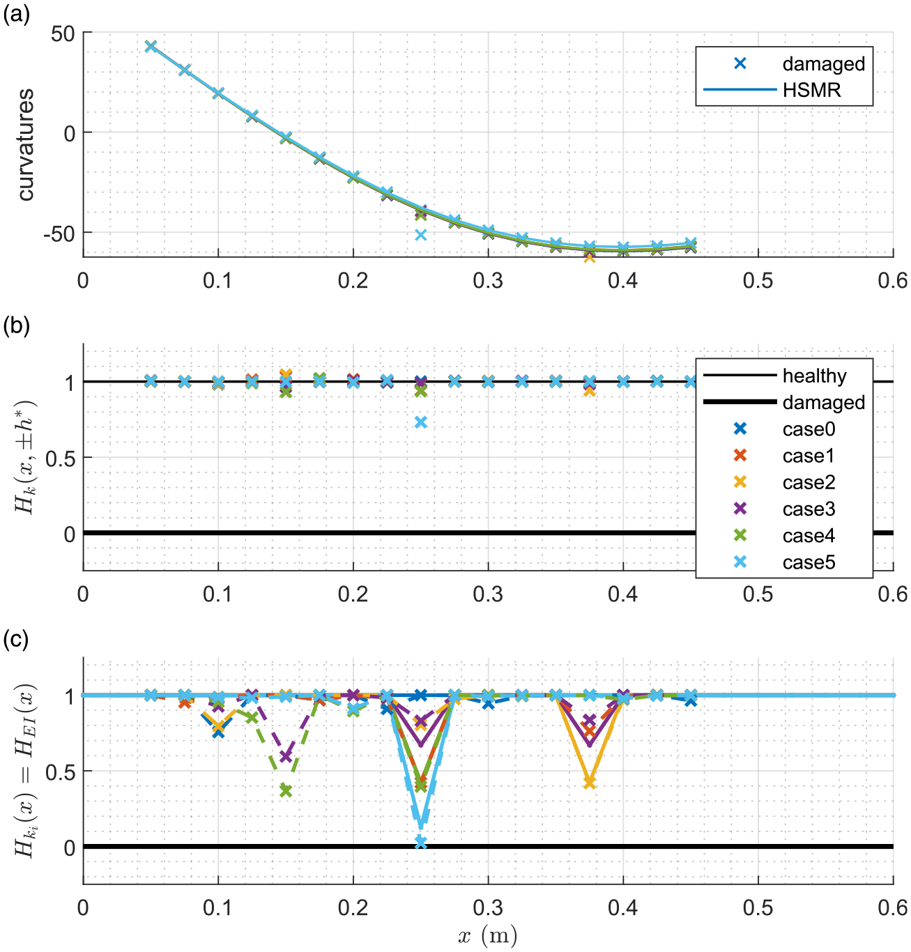In each figure: the upper chart (a) shows the curvature of the damaged structure and the HSMR synthesised from it; the middle chart (b) shows H_k(x, ±h*), calculated as the quotient of numerical derivatives; and the lower chart (c) shows $H_{k_{i}} (x)$ , which is independent on the sensor separation, calculated using the relation of equation (27) and the assumption that h_d = h_s/2.¹⁹

Figure 9.

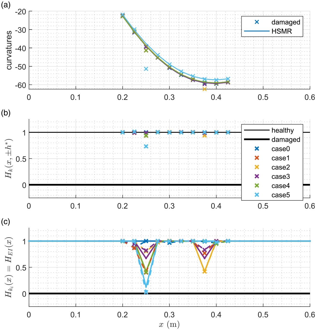
Results for the beam modelled numerically with dynamic response, D_ROI = [0.05, 0.45]. (a) Curvature of the mode shape for the damaged structure and the corresponding HSMR; (b) damage indicator H_k(x, ±h*), calculated as the quotient of numerical derivatives; and (c) damage indicator $H_{k_{i}} (x)$ , which is independent on the sensor separation (continuous lines represent actual damage, and dashed lines and crosses represent method estimations).

Figure 10.

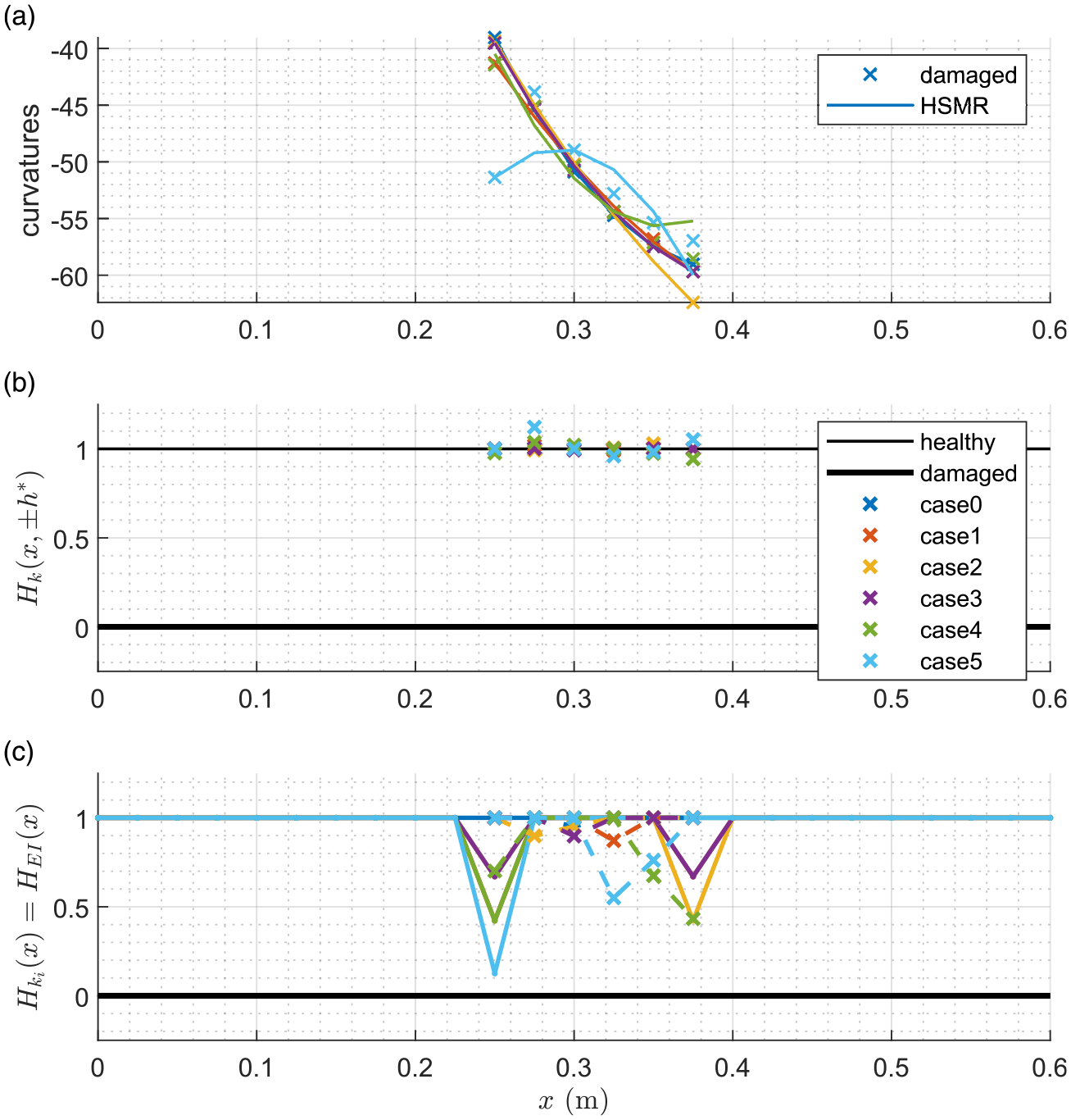
Results for the beam modelled numerically with dynamic response, D_ROI = [0.20, 0.425]. Curvature of the mode shape for the damaged structure and the corresponding HSMR; (b) damage indicator H_k(x, ±h*), calculated as the quotient of numerical derivatives; and (c) damage indicator $H_{k_{i}} (x)$ , which is independent on the sensor separation (continuous lines represent actual damage, and dashed lines and crosses represent method estimations).

Figure 11.

Results for the beam modelled numerically with dynamic response, D_ROI = [0.25, 0.375]. Curvature of the mode shape for the damaged structure and the corresponding HSMR; (b) damage indicator H_k(x, ±h*), calculated as the quotient of numerical derivatives; and (c) damage indicator $H_{k_{i}} (x)$ , which is independent on the sensor separation (continuous lines represent actual damage, and dashed lines and crosses represent method estimations).

Figure 9 shows the results of the method using a ‘large’ ROI. It can be seen that the synthesised HSMRs match the curvatures of the damaged structure perfectly in the healthy zones. Therefore, damage is estimated well at the crack locations and between them. However, large error is observed around x = 0.14 m. This is because the mode shape presents an inflexion point at that location (the support at x = 0 m is rotationally stiff and the rubber support is flexible).

That inflexion point is a zero for the curvature d_i(x) and for the bending moment f_i(x), so k_i(x) cannot be calculated accurately on its neighbourhood. Besides, the inflexion point violates the assumption of invariant sign on which equation (27) relies.

An interesting observation is that case 5 (severe single crack) has very little error even near the inflexion point. This can be explained by two causes. On the one hand, the actual change in curvature due to damage is much larger than the apparent change in curvature due to noise. On the other hand, μ(D_h) is larger than in other cases, since the crack is unique.

In the case of Figure 10, the size of the ROI is ‘appropriate’. That is, it is small enough to avoid structure discontinuities and mode shape inflexion points, while it is large enough to ensure that damage is sparse in the ROI (μ(D_h) > 0.5μ(D_ROI), equations (4) and (5). In Figure 10(a), it is evident how the robust fit rejects the outliers (points in the damaged zone). Thus, the method succeeds in detecting, locating and quantifying the damage, for single- and double-crack cases. However, it underestimates the damage when it is slight and overestimates it when it is severe (error $\approx 10 %$ ). When the crack depth is a quarter of the cross-section height (as in case 1, case 2 and case 4), the error in the estimation is close to zero. Similar error behaviour has been shown by a previously proposed quantification method which was restricted to simply supported beams only.¹⁹

Finally, Figure 11 shows the case of a ROI that is ‘too small’. It is important to note that, although the sparsity condition μ(D_h) > 0.5μ(D_ROI) is strictly valid (5 > 0.5 · 6) and there are more data points in which the structure is healthy than parameters to regress (5 > 3), these are insufficient to properly synthesise the HSMR, which can be clearly seen in Figure 11(a). Consequently, the damage could not even be detected or located (Figure 11(b) and (c)).

A possible recommendation for selecting the ROI size is simply to check the points in the chart found for H_k(x, ±h*). If most points are close to 1 and some of them are below 1, the ROI is appropriate. If several points are above 1: the ROI is too small and damage is not sparse in it, or the ROI is too large and includes inflexion points or discontinuities not considered in the HSM. This recommendation is based on the obvious fact that the stiffness cannot be greater than that of the healthy structure.

Probability of detection study

In order to show how ROI sizes and noise affect the proposed method, a probability of detection (POD) study²⁵ was carried out. POD is a frequently used quantitative measure of the capability of a nondestructive evaluation (test) for damage detection.

The study was numerically performed using the cases 0 and 4 defined in Table 1. The parameters whose influence was studied are (1) the noise level present in displacements, which propagates to curvatures and then to the damage indicators; and (2) the size of the ROI μ(D_ROI), measured as the number of points where curvature can be estimated.

In a POD study, two performance indicators are usually defined: the probability of detection, that is

POD = \frac{TP}{TP + FN};

(38)

and the probability of false alarm, that is

POFA = \frac{FP}{FP + TN};

(39)

where TP, TN, FP and FN are the number of true positives, true negatives, false positives and false negatives, respectively.

The proposed method is level 3¹; however, it can be reduced to level 1 (detection) simply by comparing H_EI(x_d) to a threshold. In this case, the flaw is expected to occur at x = x_d = L/2 with a severity H_EI(x_d) = 0.42 (see case 4 in Table 1). Damage localisation was not considered in this POD study, and detection was performed only at x = x_d = L/2 = 0.25 m. In order to balance POD and POFA, the threshold was set to the average between the healthy and damaged values of H_EI(x_d) (1.00 and 0.42, respectively), that is, at 0.71. The ROI was symmetrically defined around x_d, so only odd numbers of data points were considered.

Displacements were contaminated with white Gaussian noise N(x). Its relative level is measured using the standard definition of signal-to-noise ratio, that is

SN R_{dB} = 20 \log_{10} \frac{RMS (u_{y})}{RMS (N)} .

(40)

where RMS is the root mean square value in the ROI. When numerical differentiation is applied to the displacements, the error corresponding to that noise propagates to the estimation of curvatures. For ease of interpretation, the relative level of noise in curvatures is also measured, as follows

% noise in curvatures = 100 \frac{RMS (N^{''})}{RMS (u_{y}^{''})} .

(41)

The parametric study covered 20 noise levels (between clean signal and SNR_dB = 65 dB), 8 ROI sizes (between 3 and 17 curvature data points) and 2 cases (damaged and healthy). Each combination was run 100 times to construct statistics to apply equations (38) and (39).

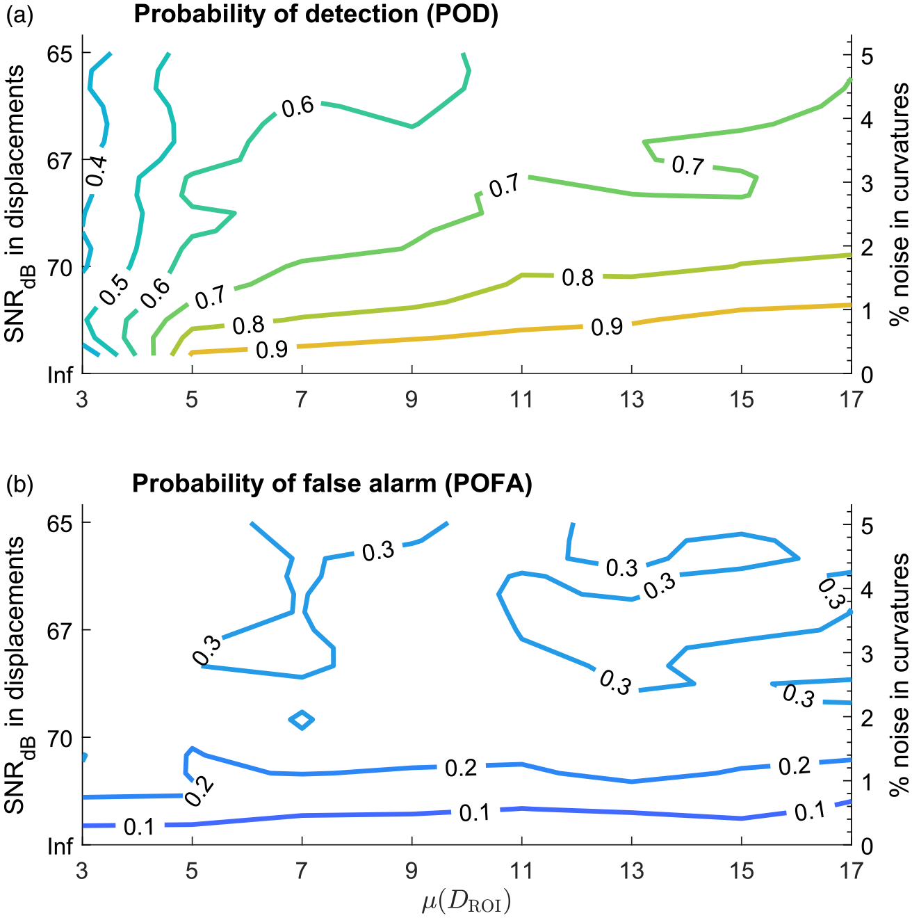
The results for POD are shown in Figure 12(a). It can be seen that using a ROI of only 3 points leads to a POD lower or equal to 0.5; that is, the method is ineffective to detect damage. However, 5 points are sufficient to achieve high PODs $(> 0.9)$ for low levels of noise. Since the iso-probability contour lines in Figure 12(a) have positive slopes (in general), an increment in the level of noise can be compensated (to some extent) by using more points in the ROI. It is worth mentioning that this is because the damaged zone is the same, so the larger the ROI, the sparser the damage. If additional defects were included by increasing the size of the ROI, a different behaviour could be obtained.

Figure 12.

(a) Probability of detection and (b) probability of false alarm, for different combinations of ROI sizes and noise levels, computed from cases 0 and 4 defined in Table 1. Each colour represents an iso-probability contour line.

In the studied case, an inflexion point is included in the ROI for μ(D_ROI) ≥ 11 (which can be seen as a zero crossing at x = 0.14 m in Figure 9(a)). Figure 12(a) shows that this does not produce any significant change in the behaviour of the POD. In other words, the inclusion of inflexion points in the ROI deteriorates performance near that points (as shown in Figure 9(c)) but not in the rest of the ROI (recall that detection was performed only at x = 0.25 m).

Regarding POFA, Figure 12(b) shows that it increases with noise (as expected). However, the POFA is practically independent of the ROI size. This is evidenced by the negligible slope of the iso-probability contour lines in Figure 12(b), especially for low noise levels. This independence can be explained by the fact that equation (39) operates only over the healthy cases, where the sparsity condition μ(D_h) >> 0.5μ(D_ROI) is trivially met.

Experimental example using static response

In this subsection, the proposed method is assessed experimentally using a statically loaded beam.

In order to obtain an accurate estimation of the beam curvature in many points, Nylon 6 was selected as the beam material, for its great tensile strength (78 MPa) and flexibility (E = 2.6 − 3.0 GPa), while plane photogrammetry was used as measurement method, for its availability and versatility.

The experimental setup is schematised in Figure 13. The beam was 1.2 m long and had a square cross-section of 0.02 m high. It was simply supported on steel angles, leading to a 1 m long free span. A single rectangular 0.005 m deep crack was induced on the beam bottom using a steel saw. The load simply consisted of a 2 kg hanging weight near the crack but outside the ROI. A single picture of the deformed cracked beam was taken with a camera, Nikon COOLPIX L310. Beam transverse displacements were then estimated by processing the resulting image with Matlab as described below.

Figure 13.

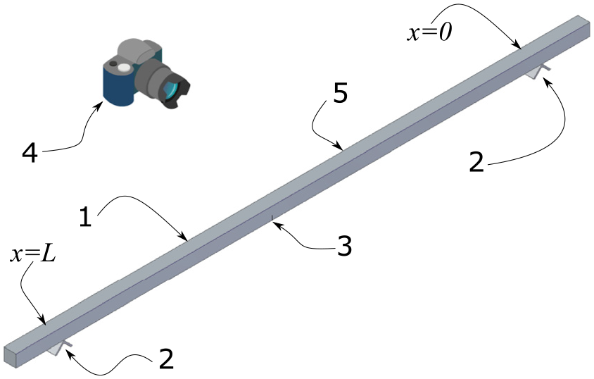
Experimental setup for the beam under concentrated static load. References: 1. beam; 2. steel angles for supporting the beam; 3. crack; 4. camera and 5. load application point.

First, the grey-scale image shown in Figure 14 was obtained by combining the 3 8-bit colour channels into a single double-precision 300 × 3000 matrix of intensity values. Then, the smooth gradient (with σ = 3) was calculated along the vertical direction to detect edges. Instead of applying the classical threshold technique, sub-pixel resolution gradient peaks were estimated and located by using cubic splines for each image column. Finally, a piece-wise linear function was fitted using the peak locations as sample points and their amplitudes as weights in a series of weighted least-squares fittings. Each piece of this piece-wise linear function correspond to an image window of, for example, 300 × 300 pixels.

Figure 14.

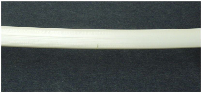
Image taken on the ROI.

This way, the transverse displacements could be estimated at 10 sample points (virtual sensors) with a precision high enough to apply the central difference numerical derivative formula and thus obtain useful estimations of the curvature.

Obviously, the upper beam edge in Figure 14 was used only. Thus, artefacts of the self-crack (which is at the bottom) in the image are avoided in the image processing.

In practice, the ROI is selected manually (using a graphical user interface) from the image and the windows are uniformly distributed along the horizontal direction depending on the desired number of virtual sensors. Therefore, in general, the window size is different from the example of 300 × 300 pixels windows.

Since the load was concentrated at a single point, the ROI was chosen to avoid that point (see Figure 14). Along this ROI, equation (21) can be used with q(x) = 0 and, therefore, p₁ need not to be fitted.

It is of note that the actual values of the applied load, load application location, support flexibility and displacements scaling are irrelevant to the proposed method, assuming the beam is in the linear elastic range. Note also that displacements and positions can be measured in units of pixels (px) and need not to be transformed to units of m.

As previously discussed, the quotient of numerically estimated curvatures is a better approximation of the reduction in mean stiffness (H_k(x, ±h*)) than of the reduction in point-wise stiffness $(H_{k_{i}} (x))$ . Therefore, such a quotient is sensor-separation-dependent and, consequently, does not quantifies the damage properly. However, $H_{k_{i}} (x)$ can be found from H_k(x, ±h), by using the relation of equation (27) and making the assumptions on which it relies.

In order to demonstrate that fact, two different sensor separations were considered, using the same image: h = 507 px (see Figure 15) and h = 331 px (see Figure 16). Both figures display numerical curvatures, H_k(x, ±h*) (from equation ( $H_{k_{i}} (x)$ (from equation (27)).

Figure 15.

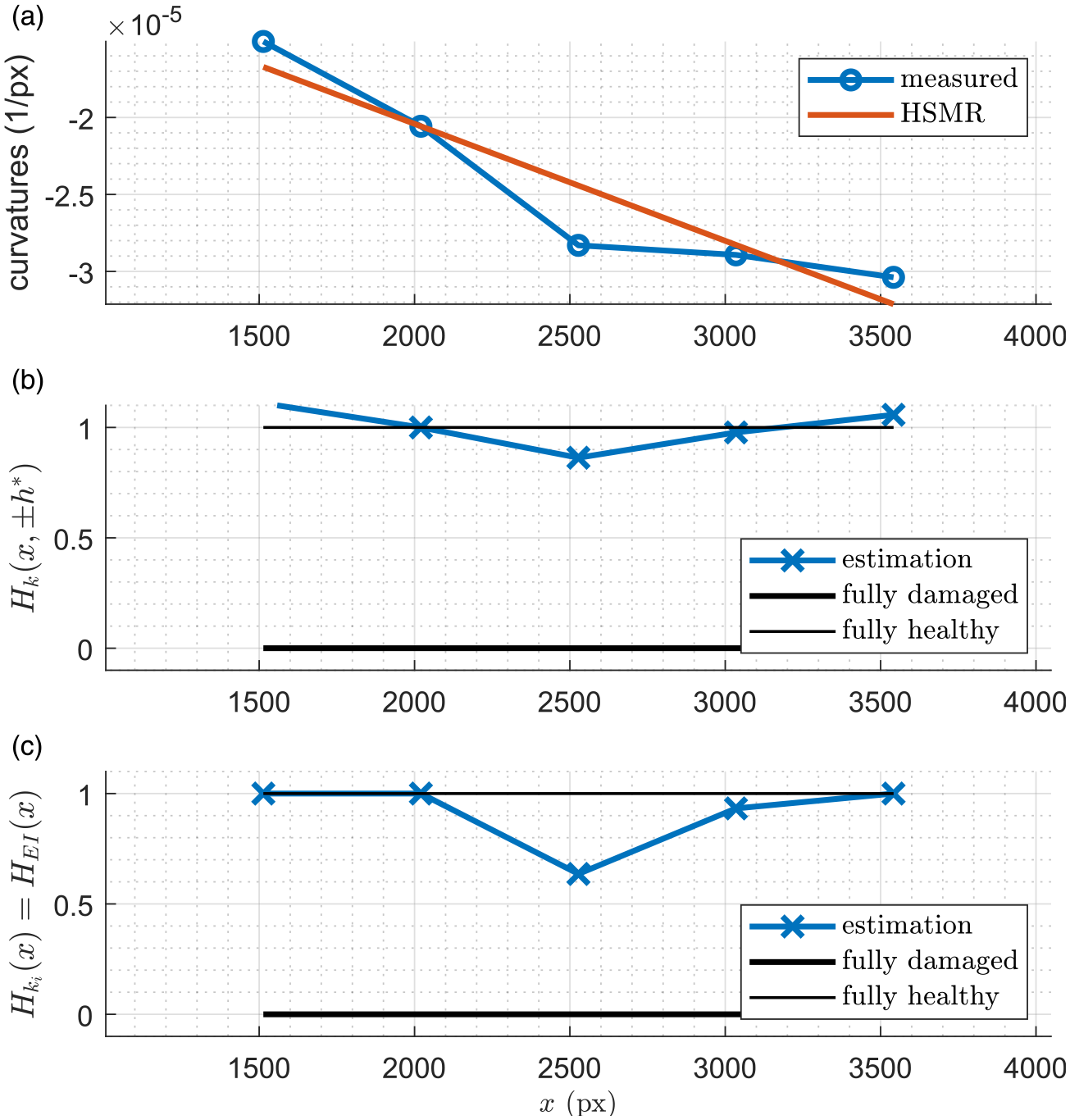
Results of the proposed method for the statically loaded beam, using h* = h/2 = 253.5, h_d = h_s/2 = 165.5.

Figure 16.

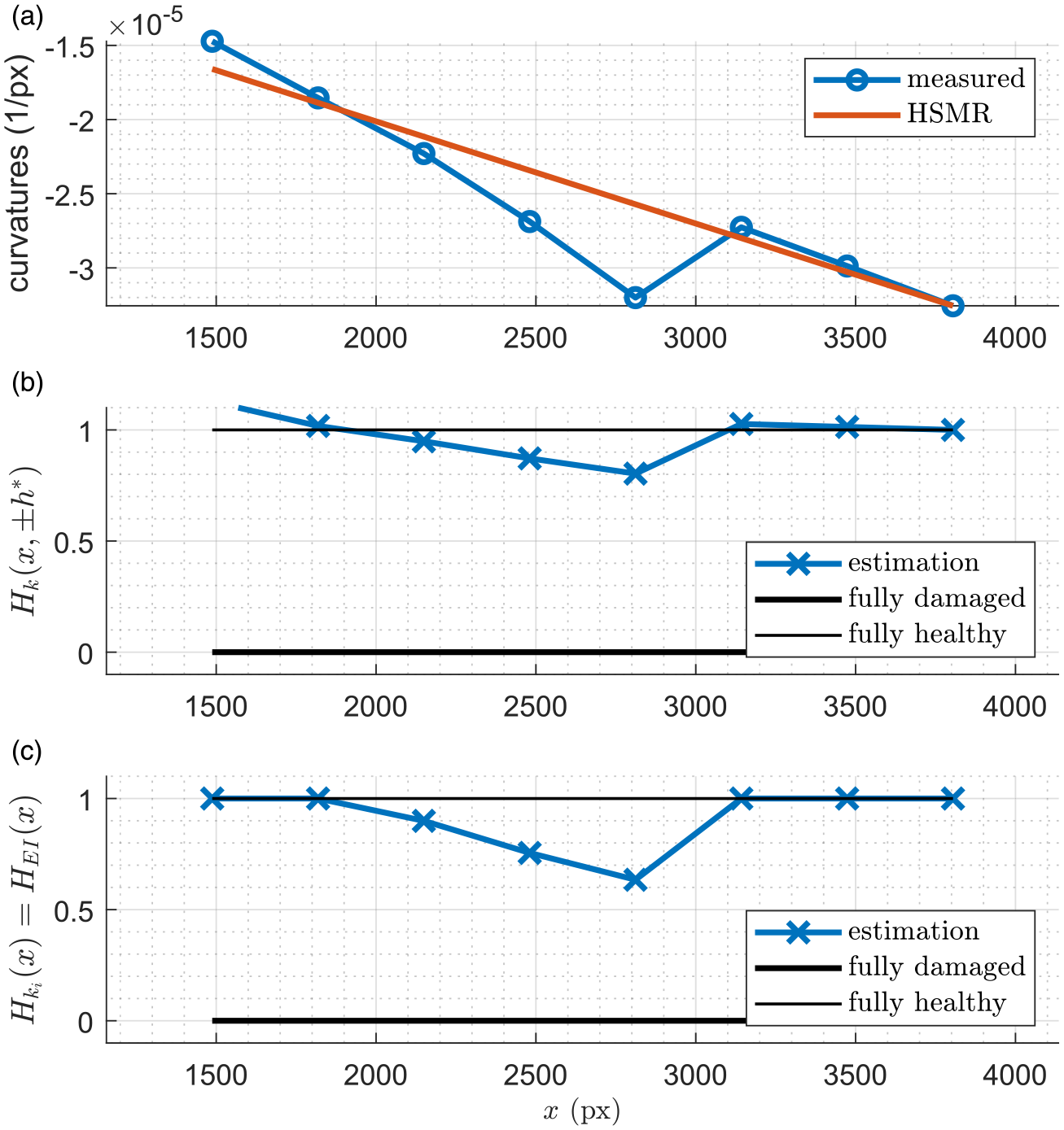
Results of the proposed method for the statically loaded beam, using h* = h/2 = 165.5, h_d = h_s/2 = 165.5.

In the image domain, the beam height is 331 px, so the apparent damage extent is 331 px (recall the relation 2h_d = h_s, empirically verified in ref. 19).

An estimation of the actual damage can be made from geometrical considerations using equation (37), which gives min(H_EI(x)) = 0.42.

Figure 15 shows a case where the averaging interval is longer than the apparent damage extent. The expected curvature for a uniform beam with concentrated load is an affine function if the ROI excludes the load application points. In this case, since the beam is not uniform due to the damage, the curve departs from the straight line at the crack location, and around it. Figure 15(a) shows this, along with the synthesised HSMR, where the latter is a straight line.

Since the number of healthy points is large enough (μ(D_h) = 4, μ(D_ROI) = 5), as compared to the number of parameters to fit (n_ip + n_ep = 0 + 2), the HSMR is found successfully. This allows to detect and locate damage, as shown in Figure 15(b). The relatively low sensitivity of H_k(x, ±h*) to the damage is due to the relatively high relation between the averaging interval length 2h* = 507 px and the apparent damage extent 2h_d = 331 px.

In Figure 15(c), the sensor-separation-independent damage indicator H_EI(x) is displayed. It can be seen how the use of the relation stated in equation (27) increases the sensitivity of the method. Nevertheless, there is still some difference between the expected value min(H_EI(x)) = 0.42 and the reached value 0.64.

Figure 16 shows a case where the averaging interval is equal to the apparent damage extent. Again, since the beam is not uniform due to the damage, the curve departs from the straight line at the crack location, and around it. Figure 16(a) shows this, along with the synthesised HSMR, where the latter is a straight line. It can be seen that the measured curvature is not exactly an affine function outside the damaged zone.

That is probably because the sensor separation is smaller and, therefore, the precision error of the displacement measurement is further amplified by the numerical differentiation formula.¹⁹ This is a disadvantage of small sensor separations. On the other hand, when comparing Figure 16(b)Figure 15(b), it can be seen that the sensitivity of H_k(x, ±h*) is higher in Figure 16(b), which is an advantage of small sensor separations.

Finally, when H_EI(x) is found from H_k(x, ±h*) and displayed in Figure 16(c), it is clear that practically the same value of min(H_EI(x)) is found, that is, 0.63 (compare Figures 15(c) and 16(c)). This is an evidence that the relation of equation (27), and the assumptions on which it relies, are valid and useful to quantify damage with independence of the sensor separation.

Conclusions

In this work, a simple method was proposed to tackle typical problems of Structural Health Monitoring: uncertainty in the boundary conditions, the need for a calibrated numerical model of the structure in its healthy state, and variability due to environmental and operational conditions.

Similar to other previously proposed methods, this relies on the assumption of damage sparsity. However, instead of using the sparse property to be able to apply regularisation techniques, here it is used to synthesise the healthy-structure model response by robust regression.

In this way, together with the assumption of invariability of the internal forces, damage can be detected, located and quantified in any region of interest (ROI) in the structure that can be represented (in its healthy state) by a simple analytical model. Using an analytical model of the ROI instead of using the virgin structure is not only simplifying, it also gives the method the possibility of identifying construction defects in the virgin structure which are not present in the hypothetical healthy structure.

The method was proposed in general terms and then it was specialised to bars and beams with static or dynamic loading. When numerically tested under ideal conditions, the method showed to be able to detect, locate and quantify damage exactly. In some cases, it is much better than using measurements of the virgin structure, which is a very important finding. In addition, the proposed method was numerically compared to the Gapped Smoothing Method (GSM) and the Global Fitting Method (GFM). Although the proposed method has similar complexity in its formulation, it showed superior performance using the same input data.

In the particular case of a free-vibrating beam with nontrivial support conditions, the method numerically showed to be able to detect, locate and quantify one and two cracks; with no other knowledge that (1) uniformity of the healthy beam and (2) mode shape displacements of the damaged beam in the ROI. It was found that particular care must be taken in the selection of the ROI: it has to be large enough to achieve a successful robust regression; while it must avoid both: structure and load discontinuities, and mode shape inflexion points. However, a POD study showed that the inclusion of inflexion points in the ROI does not affect performance far from them. Moreover, performance deteriorated because of noisier displacements can be recovered by using larger ROI sizes.

The method was also tested experimentally. In this case, a statically loaded beam was measured by using sub-pixel photogrammetry techniques and a semi-professional camera. Despite the extreme simplicity of the experimental setup, the method was able to detect and locate damage due to a single crack, and to quantify it with an error $\approx 22 %$ .

The specialisation and testing of the method using other internal forces, such as torsion or shear, and its extension to 2D structural elements and coupled internal forces are proposed as interesting future works.

Footnotes

Acknowledgements

The authors would like to thank the Argentine National Research Council (CONICET) and National University of Cuyo for the financial support. The help received from Eng. José Morán during the preparation of the figures is also gratefully acknowledged.

Declaration of conflicting interests

The author(s) declared no potential conflicts of interest with respect to the research, authorship, and/or publication of this article.

Funding

The author(s) received no financial support for the research, authorship, and/or publication of this article.

ORCID iD

Hernán Garrido

Notes

References

Rytter

. Vibrational Based Inspection of Civil Engineering Structures. PhD thesis. Aalborg, Denmark: Aalborg Universitet, 1993.

de Almeida Cardoso

Cury

Barbosa

, et al. Unsupervised real-time SHM technique based on novelty indexes. Struct Cont Health Monit2019; 26(7): 1–18. DOI: 10.1002/stc.2364.

Alves

Cury

Roitman

, et al. Novelty detection for SHM using raw acceleration measurements. Struct Cont Health Monit2015; 22(9): 1193–1207. DOI: 10.1002/stc.1741.

Tondreau

Deraemaeker

. Local modal filters for automated data-based damage localization using ambient vibrations. Mech Syst Signal Proc2013; 39(1–2): 162–180. DOI: 10.1016/j.ymssp.2013.03.020.

Surace

Bovsunovsky

. The use of frequency ratios to diagnose structural damage in varying environmental conditions. Mech Syst Signal Proc2020; 136: 106523. DOI: 10.1016/j.ymssp.2019.106523.

Park

Kim

, et al. Evaluation of bridge support condition using bridge responses. Struct Health Monit2019; 18(3): 767–777. DOI: 10.1177/1475921718773672.

Peeters

De Roeck

. One-year monitoring of the Z24-Bridge: environmental effects versus damage events. Earthquake Eng Struct Dyn2001; 30(2): 149–171.

Curadelli

Ambrosini

. Damage detection in elevated spherical containers partially filled with liquid. Eng Struct2011; 33(9): 2708–2715. DOI: 10.1016/j.engstruct.2011.05.023.

Titurus

Friswell

. Regularization in model updating. Int J Numer Met Eng2008; 75(4): 440–478. DOI: 10.1002/nme.2257.

10.

Hou

Xia

Bao

, et al. Selection of regularization parameter for l1-regularized damage detection. J Sound Vib2018; 423: 141–160. DOI: 10.1016/j.jsv.2018.02.064.

11.

Ding

Hao

. Non-probabilistic method to consider uncertainties in structural damage identification based on Hybrid Jaya and Tree Seeds Algorithm. Eng Struct2020; 220(April): 110925. DOI: 10.1016/j.engstruct.2020.110925.

12.

Rose

Wang

. Inverse methods for quantitative assessment of delamination damage based on vibrational response. Struct Health Monit2015; 14(5): 411–425. DOI: 10.1177/1475921715591874.

13.

Pitchai

Saravanan

Goswami

. Mechanics-based algorithms to determine the current state of a bridge using quasi-static loading and strain measurement. Struct Health Monit2019; 18(5–6): 1874–1888. DOI: 10.1177/1475921718815803.

14.

Zaurin

Catbas

. Structural health monitoring using video stream, influence lines, and statistical analysis. Struct Health Monit2011; 10(3): 309–332. DOI: 10.1177/1475921710373290.

15.

Ratcliffe

. Damage detection using a modified laplacian operator on mode shape data. J Sound Vib1997; 204(3): 505–517. DOI: 10.1006/jsvi.1997.0961.

16.

Yoon

Heider

Gillespie

, et al. Local damage detection with the global fitting method using mode shape data in notched beams. J Nondestr Eval2009; 28(2): 63–74. DOI: 10.1007/s10921-009-0048-6.

17.

Lai

Nagarajaiah

. Semi-supervised structural linear/nonlinear damage detection and characterization using sparse identification. Struct Cont Health Monit2019; 26(3): 1–19. DOI: 10.1002/stc.2306.

18.

Shi

Spencer

Chen

. Damage detection in shear buildings using different estimated curvature. Struct Cont Health Monit2018; 25(1): 1–20. DOI: 10.1002/stc.2050.

19.

Garrido

Domizio

Curadelli

, et al. Numerical, statistical and experimental investigation on damage quantification in beams from modal curvature. J Sound Vib2020: 485. DOI: 10.1016/j.jsv.2020.115591.

20.

El-Gebeily

Khulief

. Identification of wall-thinning and cracks in pipes utilizing vibration modes and wavelets. Appl Math Modell2016; 40(9–10): 5335–5348. DOI: 10.1016/j.apm.2015.12.031.

21.

Ferreira

AJM

. Matlab Codes for FEA. USA: Springer, 2008, p. 157.

22.

Garrido

Curadelli

Ambrosini

. A heuristic approach to output-only system identification under transient excitation. Expert Syst Appl2017; 68: 11–20. DOI: 10.1016/j.eswa.2016.10.007.

23.

Taylor

. An Introduction to Error Analysis. 2nd ed.Sausalito: University Science Books, 1997. 0-935702-42-3.

24.

ANSYS. Element reference. In ANSYS Mechanical APDL. 13th ed.Canonsburg: ANSYS, Inc., 2010. p. 1450.

25.

Matzkanin

Yolken

. A Technology Assessment of Probability of Detection (POD) for Nondestructive Evaluation. August. 1890596205, 2001.