
Abstract
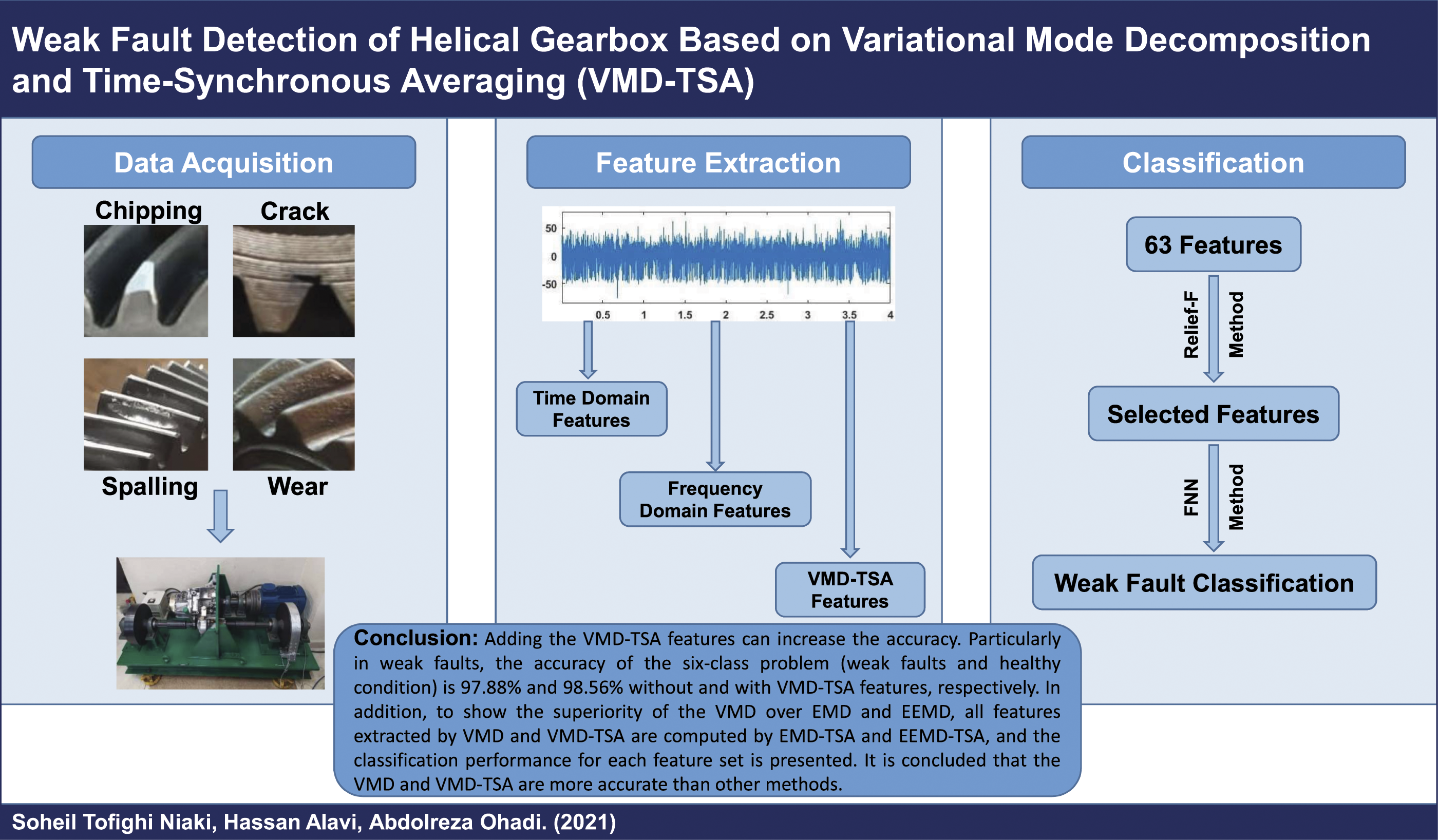
As the fault detection methods diagnose defects in the earlier stage, the subsequent costs will be reduced. Feature extraction from the vibration signal is the foremost step for incipient fault detection of gearboxes. However, the current statistical features in the time and frequency domains cannot diagnose the early or low intensity faults. In this research, for the first time, besides these features, some other features are extracted by combining variational mode decomposition and time synchronous average (VMD-TSA) to overcome the problem. The combinations have occurred in two ways. First, the Intrinsic Mode Functions (IMFs) of the TSA signal are calculated by VMD, and the Amplitude Energy (AE) and Permutation Entropy (PE) of the first four IMFs are computed. Secondly, the IMFs of vibration signals are calculated, and the TSA features are extracted from the most informative IMF. Moreover, 16 features in the time domain, 13 features in the frequency domain, and 9 features by TSA are extracted from the vibration signals. These features are extracted from healthy and four faulty conditions: crack, spalling, chipping, and wear in three different severities. After feature extraction, the Relief-F algorithm selects the informative features, and selected features are utilized for fault detection by a Feed-Forward Neural network (FNN) classifier. In this study, the ability of the VMD-TSA method is compared with others like Empirical Mode Decomposition-TSA (EMD-TSA) and Ensemble Empirical Mode Decomposition-TSA (EEMD-TSA), which shows that the proposed method is more powerful than others in early fault detection. Besides, the classification accuracy of these methods is compared with some other feature selection methods like Laplacian Score (LS), Principal Component Analysis (PCA), and Minimum Redundancy-Maximum Relevance (MRMR). Also, the performance of the FNN classifier is compared with the Support Vector Machine (SVM). As shown in this study, the VMD-TSA features improve the early fault detection in a positive manner. For instance, the classification accuracy of all features without VMD-TSA in crack fault detection is 93.98%. However, by adding VMD-TSA features, the accuracy grows up to 99.48% in the same conditions.
Keywords
Highlights
• A new method VMD-TSA is proposed to detect the helical gearbox’s incipient faults. • Experimental vibration signals have been used for the evaluation of the VMD-TSA method for incipient fault detection. • A wide range of features in time, frequency, and time-frequency domains are extracted from experimental signals, using some common features and the VMD-TSA method. • The performance of some feature selection methods is compared, and more informative features are selected from 63 ones in different domains, using the Relief-F method. • The proposed VMD-TSA method increases the accuracy of classifiers compared to not using it and outperforms the EMD-TSA and EEMD-TSA in early fault detection.
Introduction
Gearboxes are one of the main parts of rotating equipment employed to transmit the power in a specific torque and rotation speed, where may experience gear faults due to improper lubrication, overloading, and production defects. Also, the gear faults may lead to some irreparable damages. Therefore, the faults need to be detected as early as possible to reduce the maintenance cost, improve the gearbox’s operation, and prevent subsequent damages. The common faults of gears are crack, spalling, chipping, and wear, which are studied in this research.
Many methods have been used for gearbox fault detection, whereas vibration signal processing is one of the practical approaches. For example, Schmidt et al. 1 proposed a new method using instantaneous power spectrum of vibration signals. They used this method for gearbox fault detection under time-varying conditions and the method was validated by experimental testing. Another usage of vibration signals is presented by Yu et al. 2 for planetary gearbox fault detection. They modeled vibration signals as an amplitude modulation and frequency modulation (AM-FM) in resonance region to detect the faults. They also validated their theoretical calculation using numerical simulation and experimental tests. In addition to these methods, time synchronous averaging (TSA) is a classical method for gearbox condition monitoring. 3 Although the TSA can reduce noise in experimental vibration signals, it requires stationary vibration signals, which is usually impossible in many experimental cases. 4 N. Ahmed et al. 5 developed a modified TSA which was robust for gearbox fault detection under nonstationary torque and speed conditions. They proposed a Multiple-pulse Individually Rescaled-Time Synchronous Averaging (MIR-TSA) method for tooth root crack detection in spur gear. They showed that the mentioned method improves the gearbox fault detection under nonstationary conditions. Later, Jong M. Ha et al. 4 introduced an Autocorrelation-based TSA (ATSA) for condition monitoring of planetary gearboxes in wind turbines. TSA’s optimal shape and window range function were defined in the ATSA method. It helped to improve data processing efficiency and inhibition of signal distortion during the TSA. In another method, RMS based probability density function and entropy measures were used by Sharma and Parey, 6 in fluctuating speed condition. They proposed the RMS based method to boost the efficiency of entropy measures under varied speed condition.
In addition to TSA, mode decomposition methods like Empirical Mode Decomposition (EMD),
7
Ensemble Empirical Mode Decomposition (EEMD),
8
and Variational Mode Decomposition (VMD)
9
have been more utilized for fault detection. EMD is a well-known time-frequency signal decomposition method that is useful for fault detection. The EMD decomposes a signal into some IMFs containing specific frequencies. However, in some complex signals like experimental vibration signals, which contain much background noise, the IMFs may affect each other. This phenomenon is called the mode mixing problem.
10
Therefore, some approaches are proposed to alleviate the mode mixing. For example, Wu and Huang
8
proposed a new method named EEMD. The main idea of EEMD is to create an ensemble of observations by adding white Gaussian noise to the measured signal. Ensemble averaging of the extracted IMFs reduces the effects of the mode interferences. The noise amplitude and ensemble number are two critical parameters in EEMD that affect the method’s efficiency. In addition, the remaining noise in the reconstructed signals can cause lower computational efficiency.
10
To overcome these drawbacks, some other methods like Complementary EEMD (CEEMD),
11
and EMD Manifold (EMDM)
12
are proposed. Meanwhile, VMD is a noise-robust method proposed by Dragominitskiy and Zosso in 2014.
9
Some of the EMD limitations, like mode mixing problems, sampling limits, and lacks of mathematical description, have been solved. In this regard, some successful applications of VMD for fault detection are reported. Yan and Jia
13
employed VMD for rolling bearing fault diagnosis. First, they extracted features in three domains, including time, frequency, and time-frequency, that VMD computed the last one. Then, the LS algorithm was employed to select more fault-informative features. At last, Particle Swarm Optimization-based SVM (PSO-SVM) was introduced to diagnose multiple fault conditions. Y. Li et al.
14
pursued VMD to remove the noise of the vibration signals from a planetary gearbox and highlight the faults. Then, they used Generalized Composite Multi-scale Symbol Dynamic Entropy (GCMSDE) to extract the features from denoised signals. After that, the features were refined by the LS algorithm. Finally, the healthy and faulty conditions were identified by Softmax regression. In another study, J. Li et al.
15
presented a new method for impact fault detection of gearboxes. The proposed method was a combination of VMD with Coupled Underdamped Stochastic Resonance (CUSR) used to extract impulse fault features. In this study, the VMD decomposed the vibration signals into several IMFs, and then, according to the Correlation Kurtosis (CK) of each IMF, the informative IMF was selected. Finally, the impulse features were extracted by the output signal of the CUSR system. Vanraj et al.
16
used a hybrid data fusion approach by combining the EMD and Teager-Kaiser energy operator for gearbox fault detection. They extracted some statistical features from acoustic and vibration signals and then, they are sorted by order of relevance using floating forward selection method. Finally, the fault diagnosis was carried out by k-nearest neighbor classifier. In 2019, R. Gu et al.
17
proposed a method for incipient fault diagnosis of rolling bearings. The introduced method was a mixture of Adaptive VMD with Teager Energy Operator (AVMD-TEO). Firstly, the optimized parameters of AVMD, which was adopted by the grey wolf optimization algorithm, were searched. Then, the capable modal component for signal reconstruction was selected by efficient weighted kurtosis index, and at last, the reconstructed signal is processed by TEO to identify the fault frequency. In another example, Deng et al.
18
used VMD and PCA-SVM incipient fault detection of rolling bearing. The energy and kurtosis values of each IMF were calculated and then, evaluated by PCA and used as an input for SVM. The performance of this method is validated by experimental data. In the aim of early fault detection, Zhipeng Ma et al.
19
used encoder-based method to detect incipient faults for rotating machinery. They proposed an improved Gaussian process regression analysis for early fault diagnosis via encoder signals. The Gaussian process regression was modified by a spectral density complex kernel. In another research about incipient faults, Sharma and Parey
20
utilized the VMD for gearbox early fault detection under variational speed conditions. Also, the performance of VMD was compared with Empirical Wavelet Transform (EWT) and Flexible Analytic Wavelet Transform (FAWT). In continuation of using VMD, Qing Ni et al.
21
introduced a Fault Information-guided VMD (FIVMD) for rolling element diagnosis. The FIVMD method was proposed to extract the incipient bearing repetitive transients and identify the optimum bandwidth control parameter to reach the maximum fault information. Finally, comparisons with VMD, EMD, and Local Mean Decomposition (LMD) were reported, showing that the proposed FIVMD is preferable in diagnosing early bearing repetitive transients. The Fine-tuned VMD is another VMD-based method that was used for fault diagnosis of rotary machinery by Dibaj et al.
22
In this research, the values of the number of extracted modes
In addition to the aforementioned methods, some other methods like Wavelet Packet Transform (WPT), 23 wavelet energy, 24 and adaptive parameter-induced stochastic resonance 25 were employed for gearbox fault detection in different fault severities. Some other signal processing and health indicators are reviewed in Ref. [26]. However, the severities of studied faults in these methods were not incipient enough for early fault detection. In this regard, earlier faults have been introduced in this study to show the proposed method’s ability in early fault detection.
Increasing the number of features in various domains can be beneficial for gearbox fault detection and assessment of the faults in different aspects. However, some of these features can be redundant and deceptive. As a result, some feature selection methods are utilized to choose more informative features to defects. For example, Karabacak et al. 27 proposed an intelligent feature selection and classifier method for worm gear fault diagnosis. They considered wear, pitting, and tooth breakage as gear faults. They extracted some features based on vibration, sound, and thermal image data and then, classify the faulty and healthy conditions using SVM and ANN. One of the other feature selection methods is MRMR. The MRMR algorithm finds a feature subset containing distinct features. 28 The two main conditions of this algorithm are defined with mutual information, and the combination of these conditions is called Mutual Information Quotient (MIQ). As the amount of MIQ increases, the feature is more valuable for fault detection. The LS algorithm, which is a method developed by X. He et al., 29 is an effective solution for informative feature selection. In this method, a weight number that is based on feature variance is assigned to each feature. Due to the variance-basis of most feature selection methods, their main limitation is in multiple-class problems. The Relief-F algorithm, which is a kind of modified Relief, is suitable for two or more classes. 30 Like previous methods, a weight number is specified for each feature based on the k number of the nearest neighbor of each observation. The consideration of more than two neighbors can appropriate the method for more than two classes. Therefore, the Relief-F method is used for feature selection in this study. After that, the selected features are feed into the FNN classifier to identify all fault severities.
To sum up, fault diagnosis based on an experimental vibration signal is not as easy as a theoretical vibration signal. Measured signals are influenced by friction, lubrication between gears, load mechanism, and sensor mounting. Moreover, the measured signals are often contaminated by noise, which may overwhelm incipient faults and make fault detection more difficult. So, the classical methods like the Fast Fourier Transform (FFT), EMD, or some ordinary time and frequency features may not detect early fault as well as a severe one. One of the main differences between incipient faults and noise is that the faults are occurring at a specific frequency. However, the noise has been observed in a wide range of frequencies in vibration signals. The mentioned difference is the primary basis of the proposed method in this study which is called VMD-TSA.
In the first step of this paper, the theoretical background of the introduced method is reviewed, including VMD and TSA. Then, the feature extraction procedures are explained. For example, the equation of the time and frequency domain features, PE, AE, and TSA features are proposed. Also, the combination of VMD and TSA is explained. After the feature extraction step, the Relief-F algorithm used for feature selection in this paper is reviewed. In addition to the theoretical concepts of this paper, the experimental setup and measurement conditions are explained, and then, the classification accuracies of fault detections are reported. In addition, the results of different signal processing and feature selection methods are compared, and the conclusion is reported.
Theoretical background of the proposed method
In this section, the theoretical background of the proposed method is introduced. As mentioned in the previous section, the recommended method is based on VMD and TSA methods. Therefore, the main idea and the formulation of these methods are explained in this section.
Variational mode decomposition method
The VMD method is one of the newest mode decomposition methods was developed by Dragomiretskiy and Zosso.
9
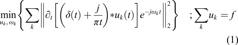
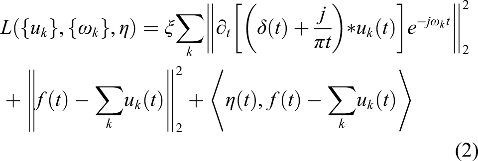
In contrast to the EMD and EEMD methods, which were experimental-based, this method is established on signal processing theories, including the Wiener filter, Hilbert transform, and signal transmission in frequency space. The primary purpose of VMD is to decompose signals into modes in which most of the valuable data is compressed at a specific frequency in each mode. This frequency is called the central frequency. The mode mixing problem, which was observed in EMD and EEMD, is rarely occurred in VMD. As a result, the frequency of defects is much better determined. The basic principle of VMD is regarded as solving the constrained variational problem, as described in equation (1)
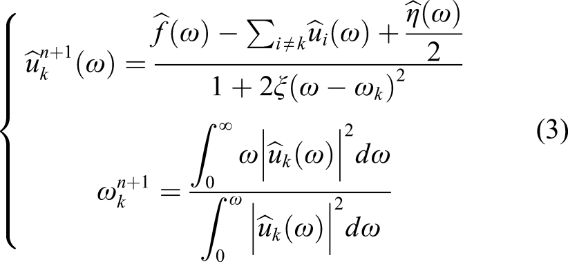
In equation (3),
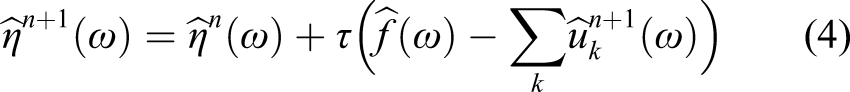
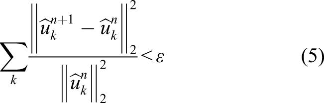
The update process is continued until the convergence criterion in equation (5) is satisfied.
Time synchronous averaging method
The original TSA method is one of the usual gearbox condition monitoring methods. The TSA divides experimental signals into The calculated signals from the time-synchronous average method in medium wear condition. (a) Experimental vibration signal (speed: 35 Hz, load: 30N.m), (b) TSA signal, (c) difference signal, (d) regular signal, and (e) residual signal.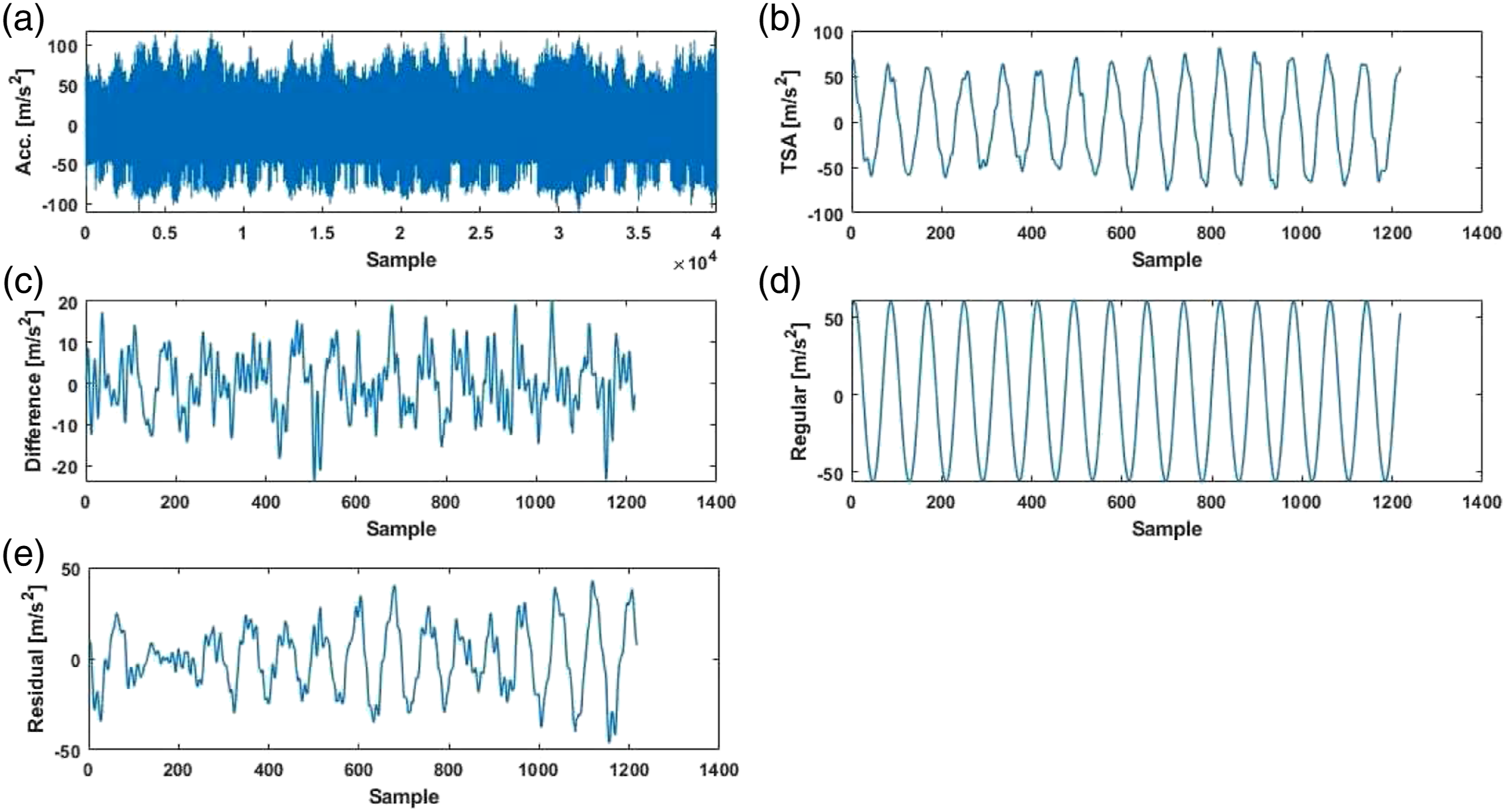
The extracted feature from the TSA method is explained in section 3.3. More details about the TSA method can be found inRef. [3].
Feature extraction
In this section, all features which were extracted from experimental signals are defined. These features are divided into four sections, including some common statistic features in the time and frequency domain (section 3.1), permutation entropy (PE), and amplitude energy (AE) from IMFs (section 3.2), TSA features (section 3.3), and VMD-TSA features (section 3.4). The first three sections were used for bearing and gearbox fault detections.5,13 However, they were not much accurate in incipient faults or early fault detection. In this study, some new features are introduced, produced by a combination of VMD and TSA. The main idea of this combination is that VMD and TSA are categories of noise-reduction methods, which help diagnose the early faults from noise. In addition, the VMD method is a kind of time-frequency method which can separate repetitive incipient faults from random noise.
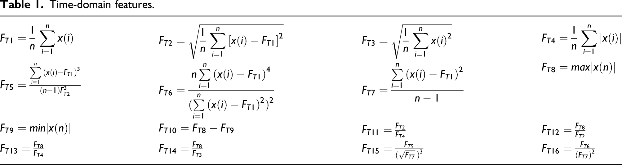
Time and frequency domain feature
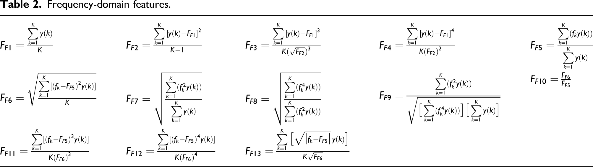
The amplitude and distribution of signals in the time-domain may be different in faulty and healthy conditions. In addition, the faults cause some new frequency components and/or change the value of existing components. So, the time and frequency domain features can be helpful in fault diagnosis. In this study, 16 time-domain and 13 frequency-domain features are extracted from vibration signals.
Time-domain features.
Frequency-domain features.
Permutation entropy and amplitude energy
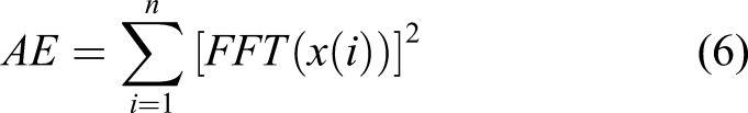
Amplitude Energy (AE) is based on FFT amplitude. Faults may lead to some peaks in the frequency domain, making a difference between healthy and faulty conditions. Equation (6) shows that the AE is computed by summing up the square FFT amplitude for each signal point
13
Permutation Entropy (PE) is a novel feature presented by Bandt and Pompep
31
that evaluates the regularity of signal and is useful for rotary machine condition monitoring.
32
For any given time signal that includes 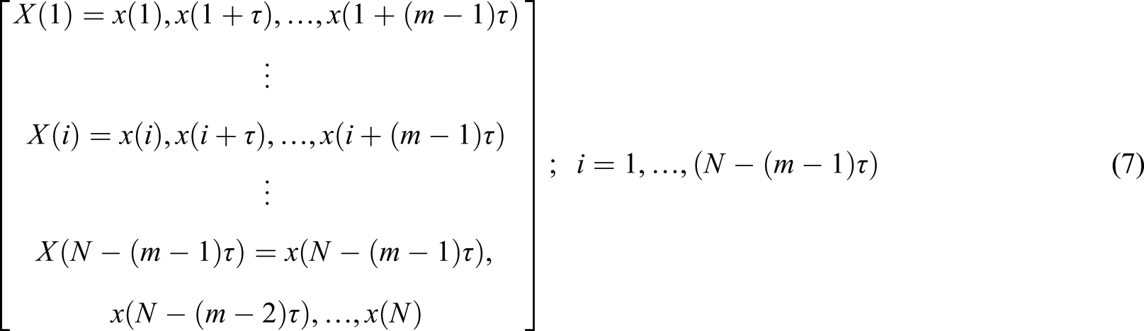
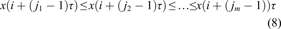
If there are two or more equivalent samples in the reconstructed section 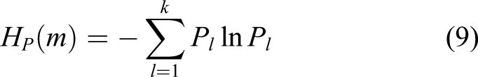
When all the symbol groups have the same probability 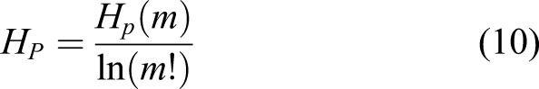
Therefore, the maximum and minimum values of
In this study, the AE and PE features are extracted from the first four IMFs of time signals obtained by the VMD method. Moreover, they are used in VMD-TSA combinations.
Time synchronous averaging features
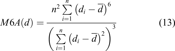
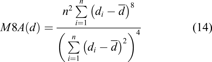
In this study, nine features are extracted from TSA, difference, regular and residual signals. Each feature is effective in diagnosing some kinds of faults. For example, the RMS is employed to evaluate the energy amplitude of the signal. The presence of localized faults increases the peakiness of vibration signals, and hence, the statistical distribution of the signal departs from the Gaussian distribution. As a result, kurtosis as a measure of non-Gaussianity will change. Also, the crest factor is a practical feature in detecting severe defects in a limited number of teeth. The crest factor is informative to high amplitude and a limited number of peaks in the signal. The RMS and kurtosis are explained in Table 1, and the crest factor is computed by equation (11)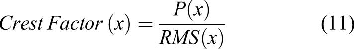
Parameter 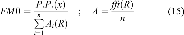
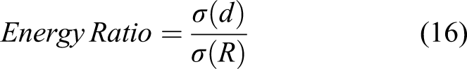
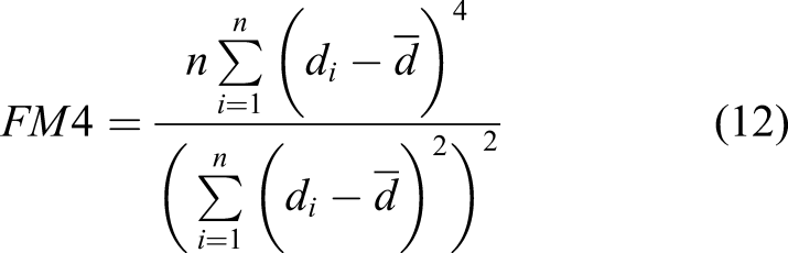
The last feature is NA4 which is computed from the residual signal. It is a modified FM4 and indicates the beginning of damage and its extension in a signal. The NA4 is calculated by equation (17)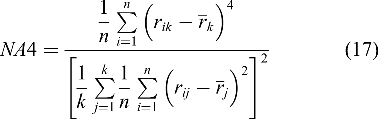
The combination of time synchronous averaging and variational mode decomposition
The main challenge in early fault diagnosis is that the fault signatures are buried in background noise and hard to be recovered. In most cases, the amplitude of the noise and incipient faults are the same in the time series and frequency spectrum. Therefore, noise-reduction methods like TSA and VMD can be suitable for early fault diagnosis. This paper proposes a new method that is made of VMD and TSA combinations. The combinations of these methods are obtained in two ways. First, the VMD method obtains the IMFs of the TSA signal, and AE and PE are extracted from the first four IMFs. The TSA features in section 3.3 are extracted from the most informative IMF of the time signal for the second way. Some techniques are proposed to choose the most informative IMF. For example, Yan and Gao
33
utilized a method based on energy measure and correction measure criteria to find the most informative mode. In another way, Wang et al.
34
selected the most informative IMF with the highest kurtosis index value. However, these methods used the time domain of the IMF and ignored the frequency domain, but they provide valuable information. In this paper, a hybrid method introduced by J. Wang et al.
12
has been used. The method is based on the kurtosis of the time and frequency domain of IMFs. The purpose of this combination is to reduce the effect of outliers. This method is named Time and Envelope Spectrum Kurtosis (TESK) and expressed by equation (18)
In conclusion, 63 features are extracted from vibration signals, categorized into three main parts: time-domain, frequency-domain, and time-frequency-domain features. These features include 16 time-domain features, 13 frequency-domain features, 8 features by VMD method, 9 features by TSA method, 8 features by the first combination of TSA and VMD, and 9 features by the second combination. In this regard, the provided experimental data are evaluated in different representation, and the loss of valuable information of faults will be reduced. It is worth mentioning that if all features fed to classifier simultaneously, the high dimensionality of input space will result in poor classification accuracies (the so-called “curse of dimensionality” effect). Therefore, the most informative features are selected by the feature selection methods and used for fault detection. The algorithm flowchart of the introduced method is shown in Figure 2. Algorithm flowchart of the introduced method.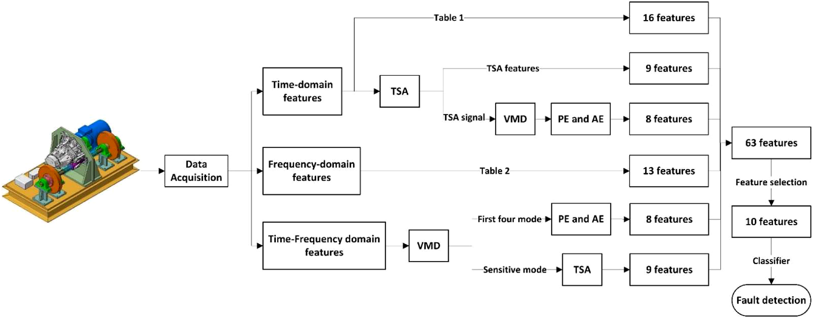
Relief-F algorithm
Many methods like LS, PCA, MRMR, and Relief-F are used for feature selection. In this paper, the performance of these feature selection methods has been evaluated accurately in detection of spalling fault severity (see Appendix 1) informative, and Relief-F as the most effective method has been selected for further investigations. The Relief-F is a kind of modified Relief method that was presented by Kononenko.
30
In the Relief method, a weight number is assigned to each feature, and whatever it increases, the feature is more potent to separate the different classes. To compute the weight number, Relief found two nearest neighbors for a random instance (
The initial value of 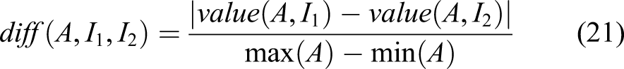
As noted in equations (20) and (21), whatever the difference between
Although the Relief can separate two different classes in a feature vector, its accuracy has decreased by increasing the number of classes. So, the Relief-F method is proposed to select the features that can separate multiple classes and increase the weight reliability, mainly in noisy conditions.
35
Both Relief and Relief-F have the same idea, but the main difference between them is that Relief-F chooses 
Each class of misses is weighted with the prior probability of that class P (C). Also, according to the third term in equation (22), which includes miss classes, the prior probability of the hit class
Experimental evaluation
Test setup description
In order to gearbox fault detection in vibration signals by the proposed method, an experimental test setup is being used, as shown in Figure 3. The test setup is designed and constructed in the Acoustics Research Laboratory at Amirkabir University of Technology.
24
It uses an AC motor (3 phase, 7.5 kW) to drive the gearbox with a pulley-belt mechanism. An inventor is used to control the rotation speed and estimate the internal torque of the electrical motor. In addition, a tachometer is used to evaluate the rotation speed of the input shaft to consider the effect of the belt slip. A cable brake is used to apply torque, and the load is controlled by changing the cable tension. Gearbox test setup and its component.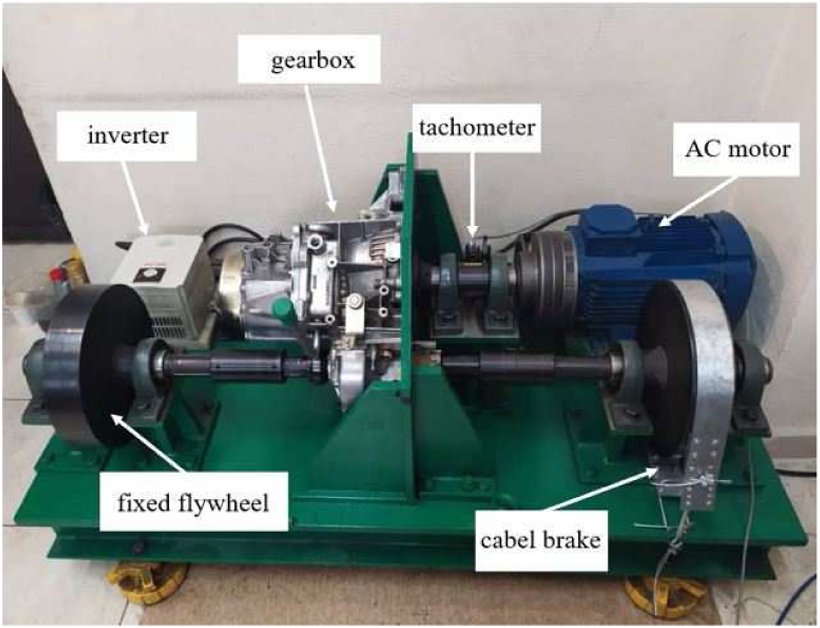
Furthermore, two uniaxial accelerometers are mounted on the gearbox, and one is mounted on the test setup. Also, the signals are collected by an A/D converter (Advantech PCI-1712, 12 bit, 1 MS/s), and then they are loaded into MATLAB (Figure 4). Three uniaxial accelerometers.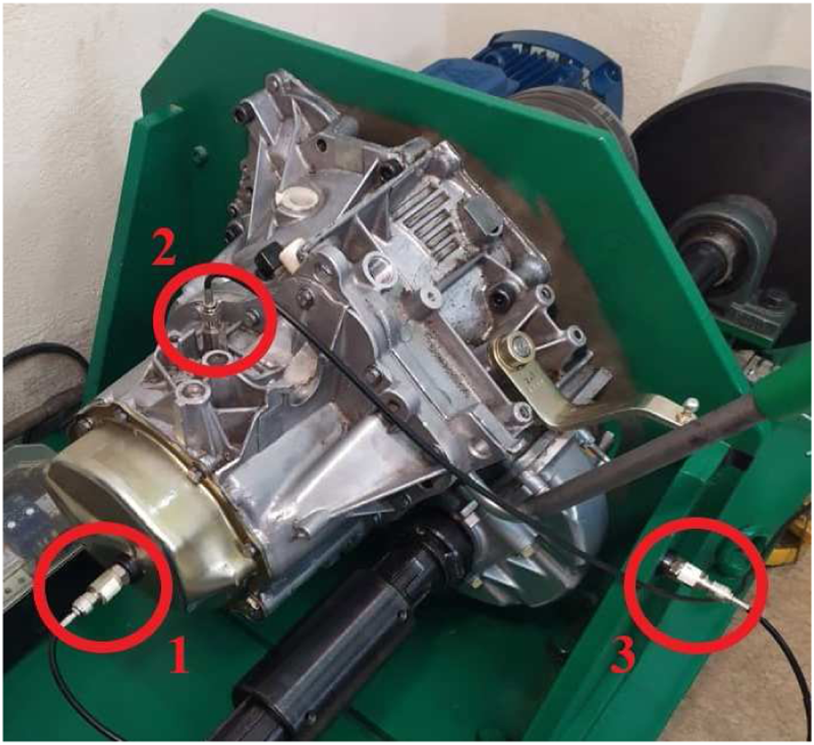
Test gears
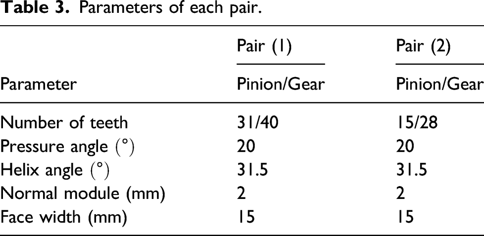
Parameters of each pair.
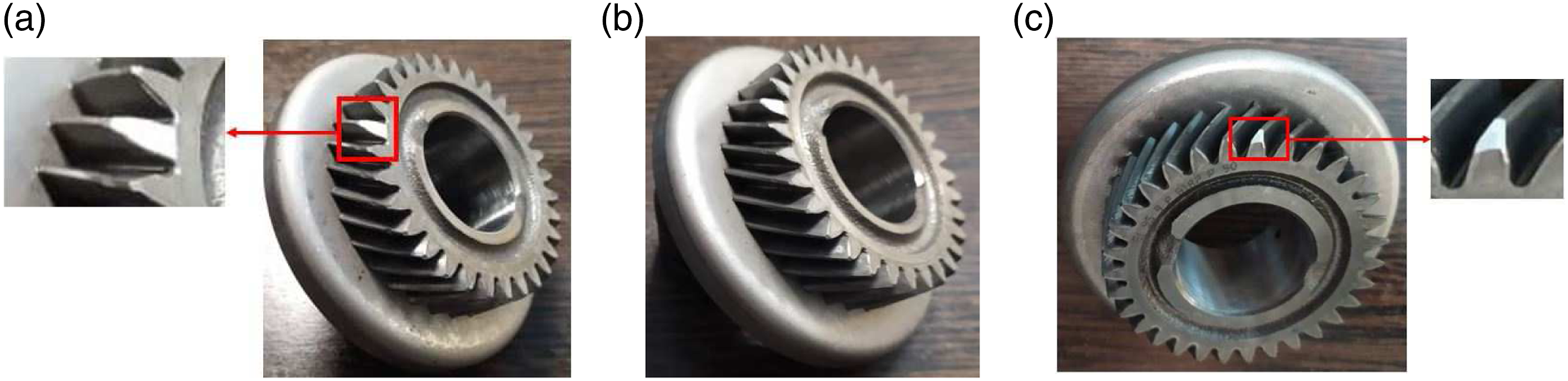
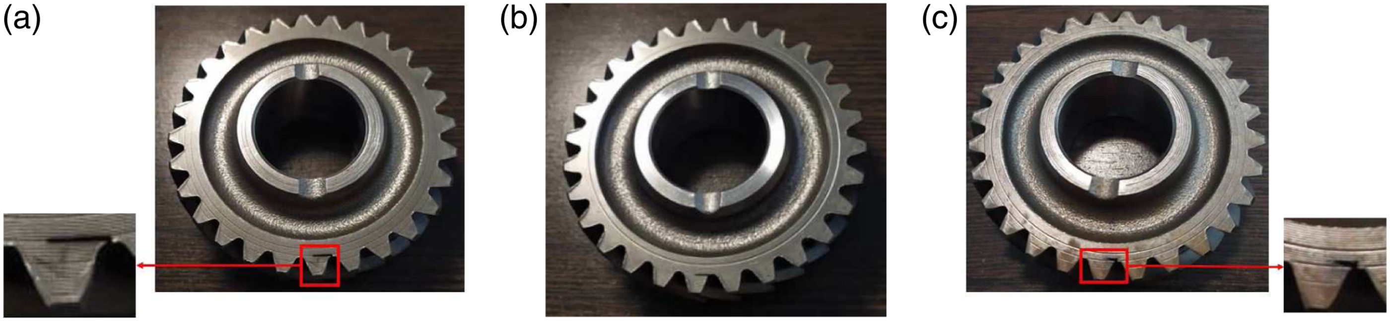
As shown in Figures 5–8, each fault is created in three different severities. A pneumatic rod grinder has been used to produce the spalling and chipping with a polycrystalline diamond drill bit. The spalling was made in one tooth as the incipient condition. The created fault is 0.9 mm in depth, and its length and width are 9 and 1.5 mm, respectively. The spalling was produced in three consecutive teeth with the same length and width as the incipient one and 0.2 mm depth in the medium fault. Finally, the severe spalling was induced in three repeated teeth, as same as the early fault. In addition, the severities of chipping are created based on the removed volume of a tooth. Thus, the early chipping is produced by 5% volume reduction, and medium and severe conditions are created by 10% and 15% volume reduction, respectively. Spalling fault on the gear of pair 1. (a) Severe fault, (b) medium fault, and (c) incipient fault. Chipping fault on the pinion of pair 1. (a) Severe fault, (b) medium fault, and (c) incipient fault. Crack fault on the gear of pair 2. (a) Severe fault, (b) medium fault, and (c) incipient fault. Wear fault on the pinion of pair 2. (a) Severe fault, (b) medium fault, (c) incipient fault, and d) healthy condition.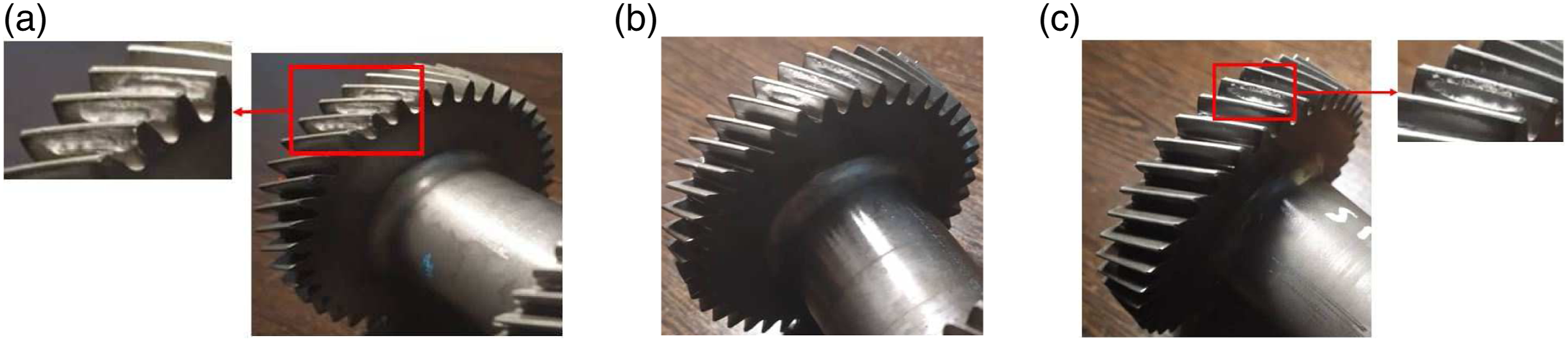
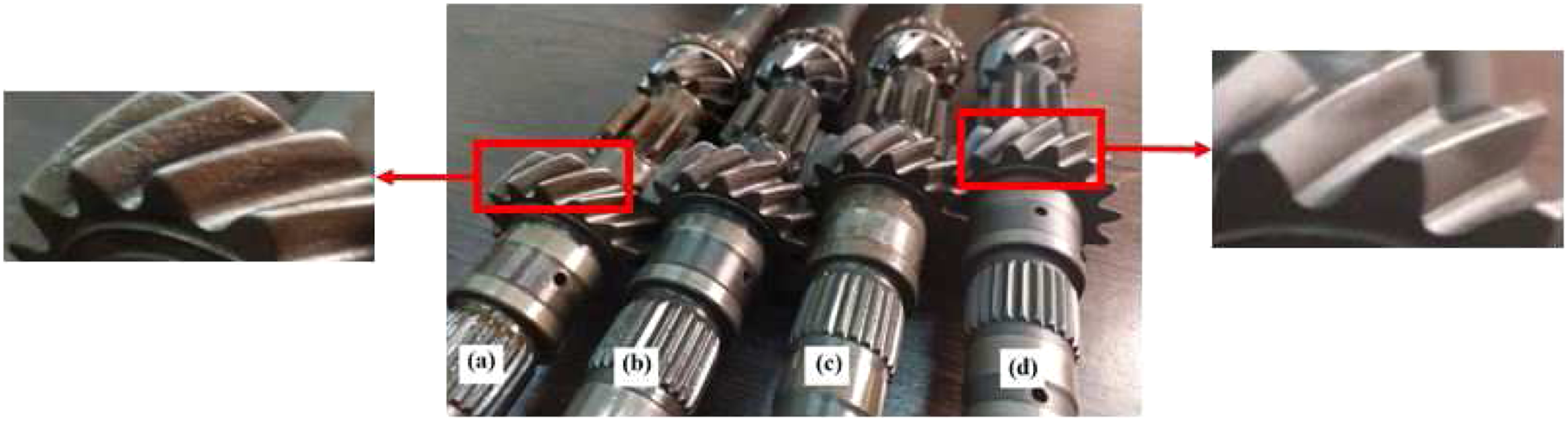
As observed in Figure 7, the crack is considered as a groove in the root of teeth, and it is created by wire cut. Also, the wear is made by electrolytic polish operation. In this process, the shaft that contains the gear is rotated uniformly, and the teeth are contacted with electrolytes. So, the wear is created uniformly in all teeth (Figure 8).
Test measurement conditions
As mentioned in section 5.1, three uniaxial accelerometers measure the vibration signals, and an A/D converter collects these signals. Signal acquisition for each test condition is performed with a sampling rate of 40 kS/s at 30, 35, and 40 Hz motor rotation speed and 35 and 45 Nm load on the motor output. Also, each test took about 10 s and was repeated three times to reduce the effect of some unknown factors which exist in experimental tests.
Experimental results and analysis
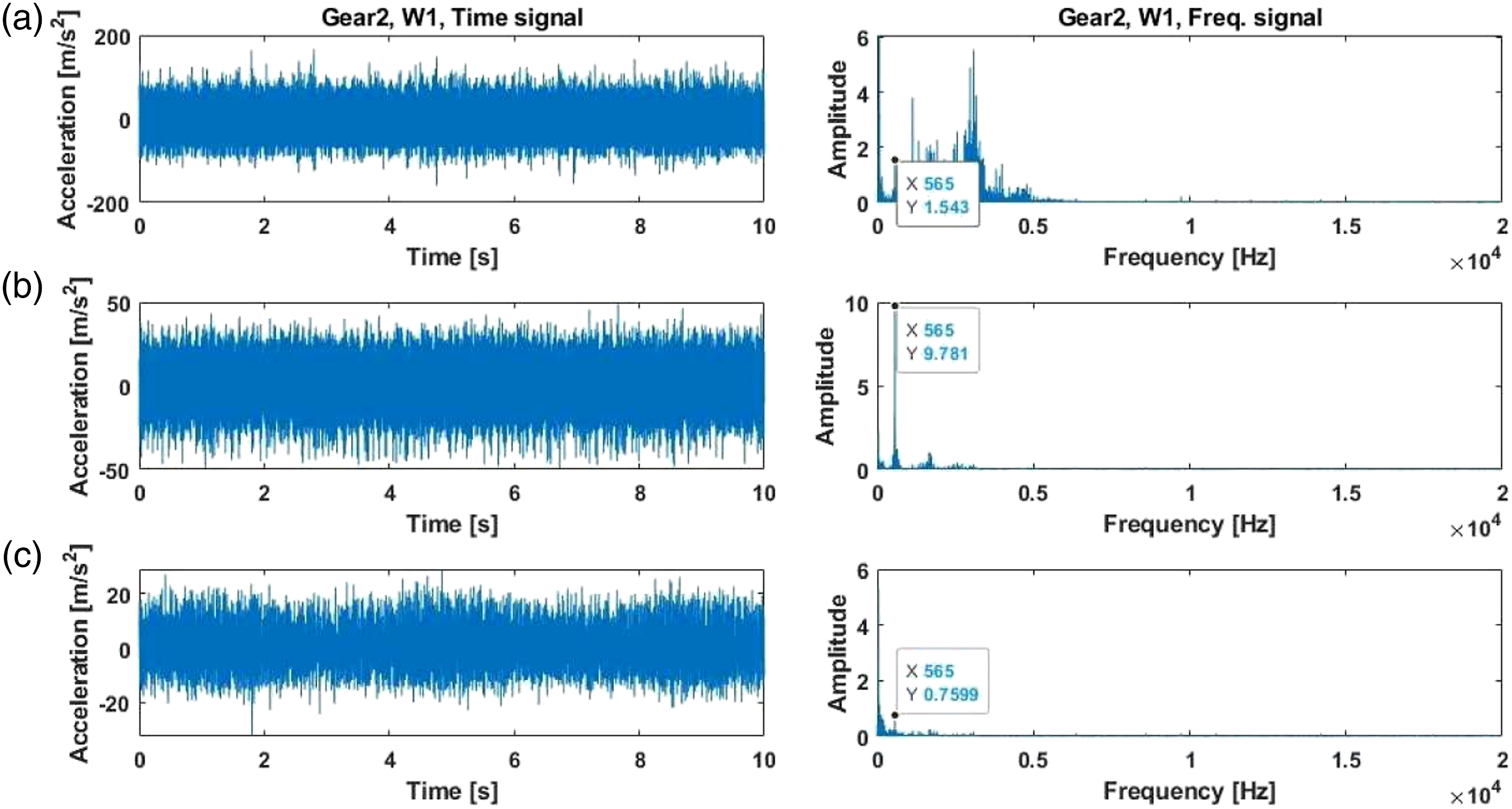
Based on the explained conditions in section 5.3, the experimental vibration signals are collected and then loaded into MATLAB. Figures 9 and 10 show that the difference between healthy and faulty conditions is not recognizable, using time-domain signals. Due to the environmental noise and test setup complexity like cable brake, pulley-belt mechanism, and gearbox operation, the fault detection might be difficult or impossible for some conditions. In Figures 9 and 10, both signals are collected at the speed of 40 Hz and the output torques 45 Nm. The mentioned points show the Gear Mesh Frequency (GMF) calculated by multiplying the number of pinion teeth and rotation speed. As explained earlier, because of the pulley-belt mechanism, the rotation speed of the input shaft is not as exact as the motor speed. So, the rotation speed is 37.6 Hz and based on Table 3, the GMF of gear pair 2 is 564.08 Hz. By comparing Figures 9 and 10, the wear and healthy signals are not much different from each other. For this reason, the VMD-TSA method is introduced to separate the healthy and early fault conditions. Experimental vibration signal of gear pair 2, in time and frequency domain for a health condition (H). (a) Accelerometer 1, (b) accelerometer 2, and (c) accelerometer 3. Experimental vibration signal of gear pair 2, in time and frequency domain for incipient wear condition (W1). (a) Accelerometer 1, (b) accelerometer 2, and (c) accelerometer 3.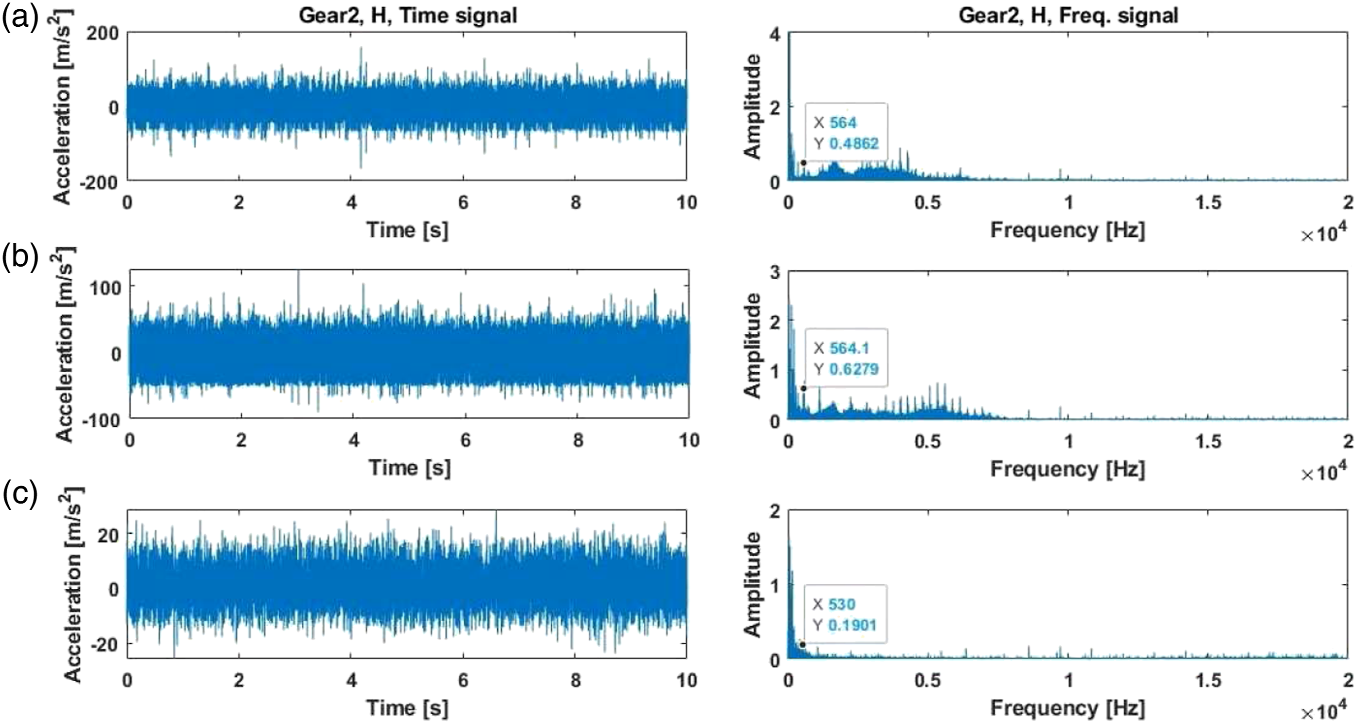
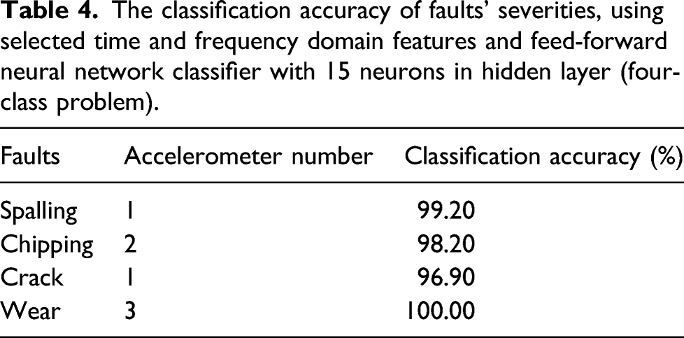
The classification accuracy of faults’ severities, using selected time and frequency domain features and feed-forward neural network classifier with 15 neurons in hidden layer (four-class problem).
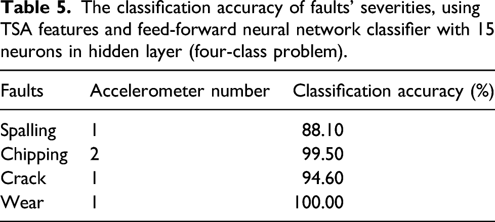
The classification accuracy of faults’ severities, using TSA features and feed-forward neural network classifier with 15 neurons in hidden layer (four-class problem).
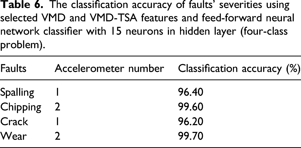
The classification accuracy of faults’ severities using selected VMD and VMD-TSA features and feed-forward neural network classifier with 15 neurons in hidden layer (four-class problem).
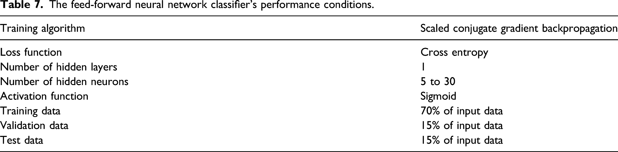
The feed-forward neural network classifier’s performance conditions.
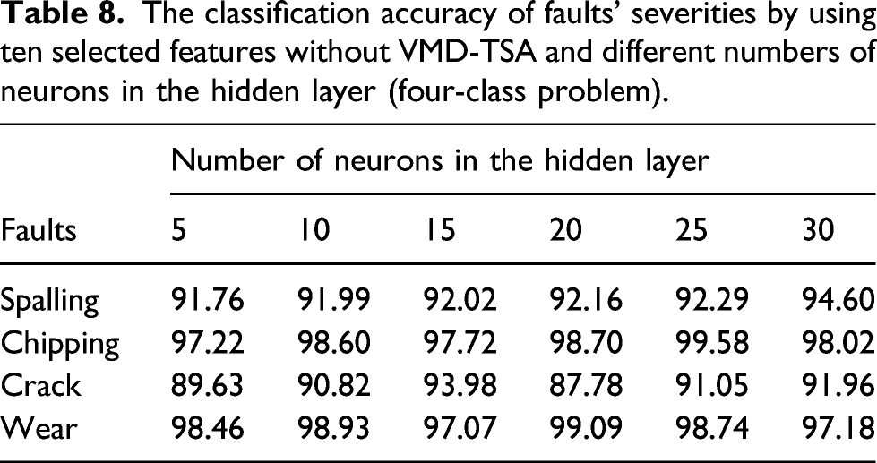
The classification accuracy of faults’ severities by using ten selected features without VMD-TSA and different numbers of neurons in the hidden layer (four-class problem).
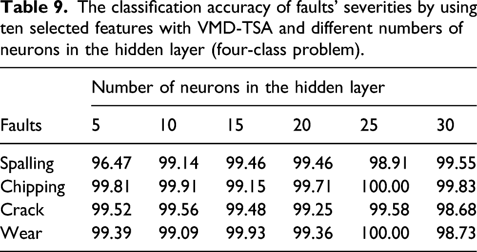
The classification accuracy of faults’ severities by using ten selected features with VMD-TSA and different numbers of neurons in the hidden layer (four-class problem).
One of the classification problems evaluated in this study is a kind of four-class problem, including three different severities of each fault and healthy condition. As shown in Table 4, the time and frequency domain features have classified the fault severities with high efficiency. The TSA features have separated the classes with acceptable accuracy, as mentioned in Table 5. In addition, the proposed VMD-TSA combinations method has achieved high performance in fault severity classification, as shown in Table 6. The different performance of classifiers in different faults is related to the intrinsic of each of them. In other words, the chief reason for the difference is based on the influence of Time-Varying Mesh Stiffness (TVMS) and Static Transmission Error (STE) as parametric and displacement excitations, respectively, on the dynamics behavior of gears. 37
Therefore, the suitable accelerometer for each part of the features and in each fault is designated. For example, in wear fault, the classification accuracy of the VMD and VMD-TSA features which are extracted from the accelerometer numbers 2, is better than other accelerometers, as shown in Table 6. So, all the 63 features are extracted from the selected vibration signals in Tables 4–6. In addition, another finding can be concluded from the results that each part of features cannot separate severities of all faults. For instance, as reported in Table 5, the accuracy of TSA features in spalling fault is not as good as other features. It shows that each feature can solve the classification problem in its view. So, it is necessary to use all features together and select a set of features that are more informative to the presence of faults. In this way, 10 features are selected by the Relief-F method, and FNN solves the same four-class problem as a classification in some different neurons in the hidden layer. To show the positive effect of the proposed VMD-TSA for improving the classification accuracy, the four-class problem is solved by all features without and with VMD-TSA features that results are reported in Tables 8 and 9, respectively. As shown in Tables 8 and 9, the classification accuracy of selected features with VMD-TSA is more than without one in all faults. For example, using the selected features without VMD-TSA and FNN with 15 neurons in the hidden layer can classify the severities of spalling with 92.02%. However, the classification accuracy with VMD-TSA features is 99.46%, in the same condition, which shows that the VMD-TSA method can increase detection accuracy.
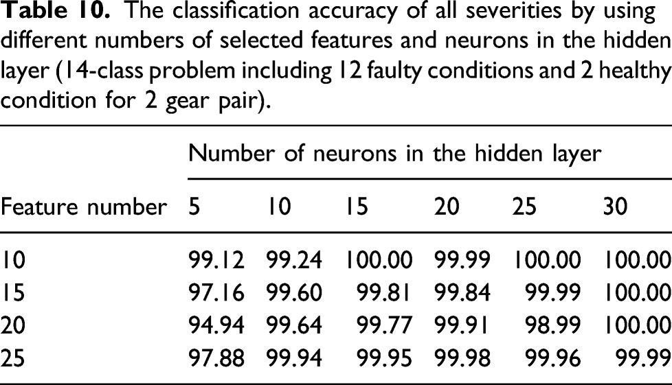
The classification accuracy of all severities by using different numbers of selected features and neurons in the hidden layer (14-class problem including 12 faulty conditions and 2 healthy condition for 2 gear pair).
The classification accuracy of incipient faults by using selected features with and without VMD-TSA and different numbers of neurons in the hidden layer (six-class problem, including four incipient severities of each kind of fault and two healthy conditions).
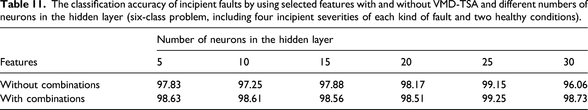
To sum it up, the extracted features by VMD-TSA combinations have a noticeable effect on improving classification accuracy, especially in incipient faults. As a result, the proposed features in this study can separate all severities of faults and classify early severities of all. It is worth to mention that the early faults are not misclassified by some benign vibrations, because the faulty situations are compared with healthy one, which the benign vibrations exist there. Moreover, in the aim of reducing misclassification, multi-domain features are extracted from the signal and the most informative features are selected for classification. In addition, as shown in Tables 4–6, all accelerometers are useful for fault detection, and each one has a different function in feature domains. However, the vibration signal which is collected by accelerometer number 1 has more valuable samples for fault detection.
Comparison among different methods
As mentioned in section 2.1, in contrast to EMD and EEMD, the VMD is a mode decomposition method based on some signal processing theories. In this section, the performance of VMD is compared with EMD and EEMD. In this way, EMD-TSA and EEMD-TSA are proposed. In these methods, the IMFs are calculated by EMD and EEMD, respectively. In addition, the support vector machine (SVM) method is exploited for classification, and the results are compared with FNN. It is worth mentioning that the performance of different feature selection methods is reported in Appendix 1.
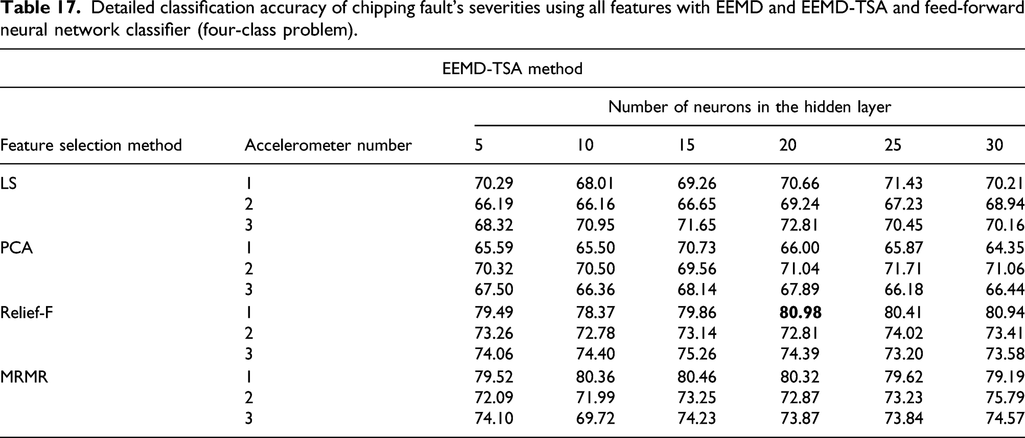
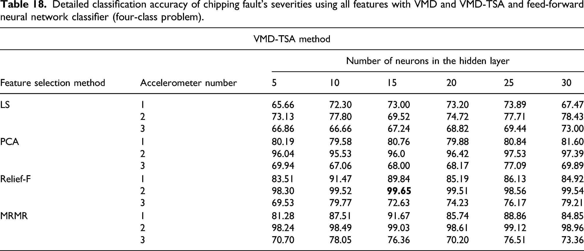
As expected, because of the mathematical base of the VMD, the VMD is more efficient than EMD and EEMD. In this regard, the FFT of the first three IMFs of the experimental signals of early chipping and healthy conditions are shown in Figure 11. As shown in Figure 11, the difference in the central frequency between faulty and healthy conditions in VMD is more recognizable than others. Therefore, the VMD method is more accurate than EMD and EEMD in early fault classification. The chief reason is that the VMD focuses on frequencies. As explained earlier, the EMD method is influenced by noise, and since the amplitude of incipient faults is trapped by noise, the EMD cannot separate the incipient faults as VMD can. In addition, in the EEMD method, adding some noise into experimental signals makes the classification more complicated than EMD. According to early faults in vibration signals, it can cause misclassification, and therefore, the classification performance is reduced. Hence, the frequency difference between noise and early faults plays a prominent role in fault detection, and this is the primary preference of the VMD over others. For more explanation, the classification accuracy of EMD-TSA, EEMD-TSA, and VMD-TSA in a four-class problem in chipping fault is reported in Appendix 2. The FFT of three first modes of early chipping (CH1) and health conditions (H). (a) VMD, (b) EMD, and (c) EEMD.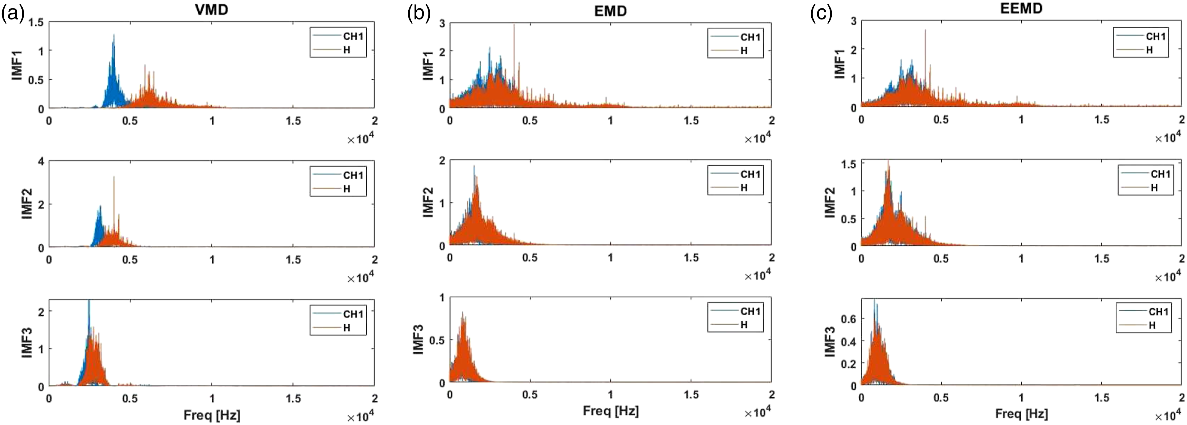
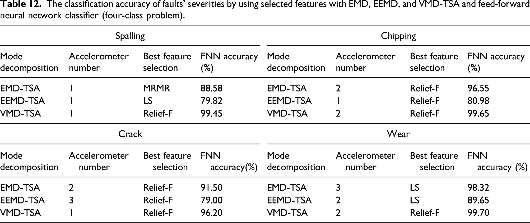
The classification accuracy of faults’ severities by using selected features with EMD, EEMD, and VMD-TSA and feed-forward neural network classifier (four-class problem).
The classification accuracy of faults’ severities by using selected features with EMD, EEMD, and VMD-TSA and SVM classifier (four-class problem).
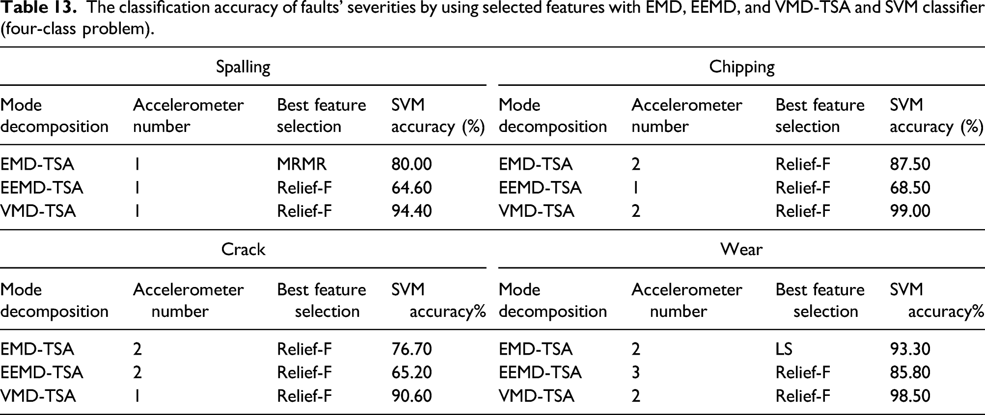
Finally, the proficiency of classification methods is appraised. As shown in Table 12 and 13, the accuracy of the FNN classifier is higher than the SVM. The SVM method natively is a binary classifier. The same principle is applied for multiclass problems after breaking down the multiclass into multiple binary classification problems. The One-vs-One and One-vs-Rest are two approaches that are used for multiple classifications. 38 However, the FNN classifier can be designed for multiple classes. Also, the difference between two classifiers in the training approach can be influential on their performance.
Some faults like crack and chipping dramatically change the TVMS of mating gears. On the other hand, wear and shallow spalls result in minor changes in TVMS while reasonably alter the STE between mating gears. Therefore, the signal pattern of each type of fault differs from the other.39,40 A proper combination of signal processing, feature extraction, and feature selection techniques can reveal the incipient signatures of faults among other components. On the other hand, classifiers like FNN could differentiate various fault signatures and classify them into correct categories.
Conclusion
This study evaluates the performance of the VMD and the VMD-TSA combinations in gearbox fault diagnosis, specifically early faults. The experimental vibration signals of gearbox for different severities of four faults under three different speeds and two different torques are acquired and analyzed with signal processing methods. In addition to VMD and VMD-TSA features, other features in time and frequency domains are extracted from vibration signals to enrich the feature set. Overall, 63 features are extracted, including nine TSA features, 16 time-domain features, 13 frequency-domain features, 8 VMD features, and 17 VMD-TSA features. Then, 10 features that are more fault-informative than others are selected by the Relief-F algorithm, and finally, fault severity is detected by the FNN classifier. As discussed, the performance of the proposed method is significant in fault severity classification, chiefly to early faults. For example, the classification accuracy of the spalling fault severity is 92.02% using all features without the VMD-TSA method and an FNN classifier with 15 neurons in a hidden layer. However, adding the VMD-TSA features can increase the accuracy up to 99.46%. Particularly in incipient faults, the accuracy of the six-class problem (early faults and healthy condition) is 97.88% and 98.56% without and with VMD-TSA features, respectively. In addition, to show the superiority of the VMD over EMD and EEMD, all features extracted by VMD and VMD-TSA are computed by EMD-TSA and EEMD-TSA, and the classification performance for each feature set is presented. It is concluded that the VMD and VMD-TSA are more accurate than other methods. In chipping fault, the classification accuracy of the VMD-TSA method using the FNN classifier is 99.65%. However, the accuracy of EMD-TSA and EEMD-TSA is 96.55% and 80.98%, respectively. Moreover, the effectiveness of the Relief-F algorithm is compared with other feature selection methods, including PCA, LS, and MRMR. It is also observed that the selected features by Relief-F are more fault-informative than other selected features. Also, the classification accuracy of the FNN method in EMD, EEMD, and VMD feature sets is much better than SVM. In crack fault, the classification accuracy of the four-class problem is 96.20%, using VMD-TSA features and FNN classifier. However, the accuracy of the SVM method is 90.60%, in the same conditions. It is worth mentioning that the performance of the FNN and SVM in some cases like crack and spalling defects are approximately the same, using VMD-TSA features. It shows that the proposed VMD-TSA method is powerful enough to detect all fault severities independent of classifier type.
Footnotes
Funding
The author(s) received no financial support for the research, authorship, and/or publication of this article.
Appendix 1
As mentioned in section 4, the performance of each feature selection method is proposed in Table 14. The four-class classification problem is solved for spalling fault’s severities using all features with VMD and VMD-TSA. As shown in Table 14, the features selected by the Relief-F method have the maximum classification accuracy compared with other methods. Detailed classification accuracy of spalling fault’s severities using all features with VMD and VMD-TSA, feed-forward neural network classifier, and different feature selection methods (four-class problem).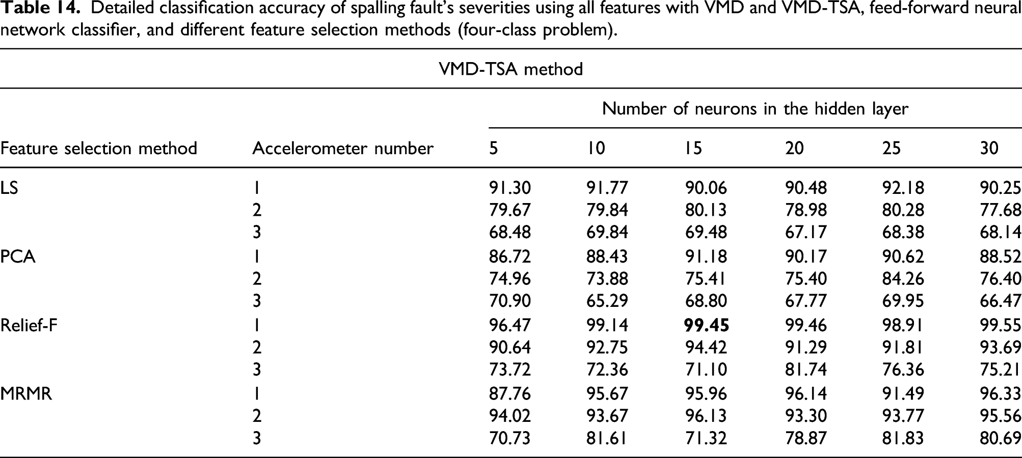
VMD-TSA method
Feature selection method
Accelerometer number
Number of neurons in the hidden layer
5
10
15
20
25
30
LS
1
91.30
91.77
90.06
90.48
92.18
90.25
2
79.67
79.84
80.13
78.98
80.28
77.68
3
68.48
69.84
69.48
67.17
68.38
68.14
PCA
1
86.72
88.43
91.18
90.17
90.62
88.52
2
74.96
73.88
75.41
75.40
84.26
76.40
3
70.90
65.29
68.80
67.77
69.95
66.47
Relief-F
1
96.47
99.14
99.46
98.91
99.55
2
90.64
92.75
94.42
91.29
91.81
93.69
3
73.72
72.36
71.10
81.74
76.36
75.21
MRMR
1
87.76
95.67
95.96
96.14
91.49
96.33
2
94.02
93.67
96.13
93.30
93.77
95.56
3
70.73
81.61
71.32
78.87
81.83
80.69
About the time consumption of feature extraction and classification, the calculation time for extracting all 63 features takes about 5 min. However, the classification time is much lower than a minute. For example, the classification time for a four-class problem (three fault intensity and healthy condition) in spalling fault is reported here in Table 15. We used an FNN classifier with 15 neurons in a hidden layer and selected different number of features using the Relief-F method from all 63 ones. Accuracies and time consumption of feed-forward neural network classifier with 15 neurons in a hidden layer in a four-class problem of spalling fault.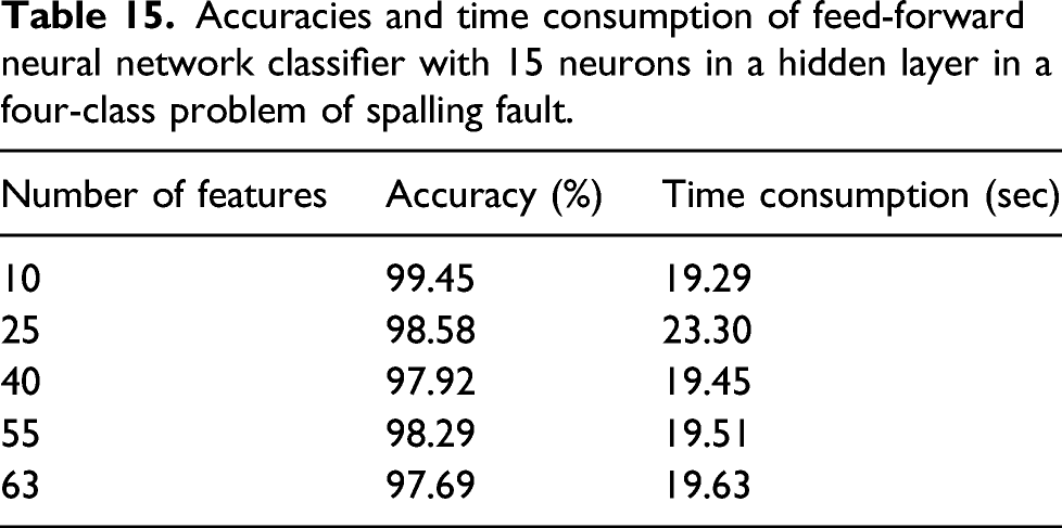
Number of features
Accuracy (%)
Time consumption (sec)
10
99.45
19.29
25
98.58
23.30
40
97.92
19.45
55
98.29
19.51
63
97.69
19.63
As shown in Table 15, there is not a remarkable difference between the time consumption of the classifier in the different number of features. However, as the number of features increases, the classifier’s accuracy is reduced, which can be a result of “curse of dimensionality” effect. So, the highest percentage of accuracy can be achieved by ten number of the most sensitive features.
Appendix 2
As explained in section 6, the maximum accuracy of EMD, EEMD, and VMD methods in all faults is reported in Tables 12 and 13. This section presents the detailed classification accuracy for each mode decomposition method using the FNN classifier and ten features selected by feature selection methods. These results belong to the chipping fault (Tables 16–18). Detailed classification accuracy of chipping fault’s severities using all features with EMD and EMD-TSA and feed-forward neural network classifier (four-class problem). Detailed classification accuracy of chipping fault’s severities using all features with EEMD and EEMD-TSA and feed-forward neural network classifier (four-class problem). Detailed classification accuracy of chipping fault’s severities using all features with VMD and VMD-TSA and feed-forward neural network classifier (four-class problem).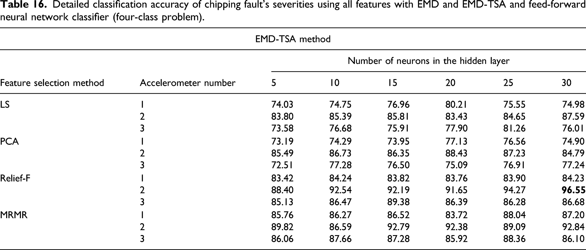
EMD-TSA method
Feature selection method
Accelerometer number
Number of neurons in the hidden layer
5
10
15
20
25
30
LS
1
74.03
74.75
76.96
80.21
75.55
74.98
2
83.80
85.39
85.81
83.43
84.65
87.59
3
73.58
76.68
75.91
77.90
81.26
76.01
PCA
1
73.19
74.29
73.95
77.13
76.56
74.90
2
85.49
86.73
86.35
88.43
87.23
84.79
3
72.51
77.28
76.50
75.09
76.91
77.24
Relief-F
1
83.42
84.24
83.82
83.76
83.90
84.23
2
88.40
92.54
92.19
91.65
94.27
3
85.13
86.47
89.38
86.39
86.28
86.68
MRMR
1
85.76
86.27
86.52
83.72
88.04
87.20
2
89.82
86.59
92.79
92.38
89.09
92.84
3
86.06
87.66
87.28
85.92
88.36
86.10
EEMD-TSA method
Feature selection method
Accelerometer number
Number of neurons in the hidden layer
5
10
15
20
25
30
LS
1
70.29
68.01
69.26
70.66
71.43
70.21
2
66.19
66.16
66.65
69.24
67.23
68.94
3
68.32
70.95
71.65
72.81
70.45
70.16
PCA
1
65.59
65.50
70.73
66.00
65.87
64.35
2
70.32
70.50
69.56
71.04
71.71
71.06
3
67.50
66.36
68.14
67.89
66.18
66.44
Relief-F
1
79.49
78.37
79.86
80.41
80.94
2
73.26
72.78
73.14
72.81
74.02
73.41
3
74.06
74.40
75.26
74.39
73.20
73.58
MRMR
1
79.52
80.36
80.46
80.32
79.62
79.19
2
72.09
71.99
73.25
72.87
73.23
75.79
3
74.10
69.72
74.23
73.87
73.84
74.57
VMD-TSA method
Feature selection method
Accelerometer number
Number of neurons in the hidden layer
5
10
15
20
25
30
LS
1
65.66
72.30
73.00
73.20
73.89
67.47
2
73.13
77.80
69.52
74.72
77.71
78.43
3
66.86
66.66
67.24
68.82
69.44
73.00
PCA
1
80.19
79.58
80.76
79.88
80.84
81.60
2
96.04
95.53
96.0
96.42
97.53
97.39
3
69.94
67.06
68.00
68.17
77.09
69.89
Relief-F
1
83.51
91.47
89.84
85.19
86.13
84.92
2
98.30
99.52
99.51
98.56
99.54
3
69.53
79.77
72.63
74.23
76.17
79.21
MRMR
1
81.28
87.51
91.67
85.74
88.86
84.85
2
98.24
98.49
99.03
98.61
99.12
98.96
3
70.70
78.05
76.36
70.20
76.51
73.36