Guided Wave SHM system for detection and quantification of damages in FPSOs storage tanks using data-driven algorithm

Abstract

In this work, we propose a data-driven method to perform detection and quantification of damage in guided wave data from Structural Health Monitoring. The data is from a full-scale panel mimicking a critical region of a Floating Production Storage and Offloading storage tank. For this, signals were initially recorded from the structure in the pristine condition to create a baseline database. Subsequently, different damage levels were introduced in the panel; we took new measurements for each damage level. Our data-driven method consists in performing a dimension reduction in these datasets using independent component analysis. The weights vectors of the independent component analysis were used to identify if a given signal came from a pristine or a damaged condition through a procedure involving statistical correlation. We obtained average accuracy rates above 90% for damage detection, with average Type I-error rates below 10% and average Type II-error rates below 35%. In addition, it was possible to quantify the severity of the damage at all depth stages.

Keywords

Data driven Structural health monitoring complex structures guided waves

Introduction

Floating Production Storage and Offloading units (FPSO) are offshore facilities for oil exploration. They allow great flexibility and operation in remote regions,¹ as they can act as an intermediate pre-processing and storage facility.² The oil from their storage tanks is periodically discharged into oil tankers for transportation and distribution.

Due to their exposure to aggressive mixtures of ballast sea water and oil, FPSO storage tanks commonly face problems related to corrosion damage.^3,4 Structural integrity is ensured through periodic inspections and maintenance routines which are expensive and time-consuming. Furthermore, the personnel involved in these procedures are exposed to risks from working in confined spaces with toxic atmospheres.⁵ A system capable of automatic corrosion detection would eliminate the need for these interventions and would be highly desirable.

The Guided Wave (GW) technique has the characteristic of monitoring extensive regions of a structure from a single access point, allowing the inspection of remote and difficult-to-access parts.^6–8 As shown in the literature, systems based on elastic guided waves have great potential for application in Structural Health Monitoring (SHM) of complex structures^9,10 with areas of difficult access.¹¹ Thus, proving to be a promising technique for application in the structure studied in this work. These systems are usually composed of an array of permanently-attached piezoelectric transducers, each one acting sequentially as emitter and receiver of the guided waves.^12,13 In this configuration, the presence of a defect will somehow modify the propagation of the waves compared with a pristine state.^14,15

The interpretation of data from such a system is commonly made directly by trained technical operators in a classical non-destructive testing (NDT) procedure. It is their responsibility to manage the structural integrity and alert when there is an abnormality. However, since SHM data is generated automatically, in much more frequent intervals than periodic NDT and as the number of monitoring locations in a structure increases, the flow of data can become unmanageable for human interpretation.¹⁶

Artificial Intelligence (AI) techniques¹⁷ is an option to solve the problem of dealing with a large volume of generated data. Thus, standing out as one of the main areas for future research.¹⁶ Among several AI techniques, dimensionality reduction algorithms can improve data analysis and reduce data complexity.¹⁸ In addition, some of these algorithms can perform feature extraction and deal with additional common problems in datasets, such as noise, complexity and sparsity.

The most representative and successful algorithms that have applications in guided wave data include, without limiting the generality of the foregoing, Principal Component Analysis (PCA),^19–21 AutoEncoder,²² Linear Discriminant Analysis (LDA),²⁰ Multi-Dimensional Scaling (MDS),²³ Singular Value Decomposition (SVD),²⁴ Locally Linear Embedding (LLE),²⁵ t-Distributed Stochastic Neighbour Embedding (t-SNE)²¹ and Independent Component Analysis (ICA).^19,24,26 Other feature extraction algorithms that are among the most representative and successful are Kernel PCA (KPCA), Isometric Mapping (ISOMAP) and Laplacian Eigenmap (LE).²⁷

Recent research shows that the application of feature extraction algorithms in guided wave SHM has great potential.²⁸ Methods have been developed for different purposes, structures and materials using dimensional reduction algorithms. In some developed methods, these feature extraction techniques were combined with other machine learning (ML) techniques.^{19,20,22,23,25} In other approaches, different feature extraction techniques were combined.²¹ In addition, some methods were developed using only one feature extraction technique.^24,26

The main goal of this work is to build a method for the detection and quantification of damage using reduced-dimensional guided wave SHM data. In addition, the approach should be able to deal with environmental variations without pre-processing techniques, for example, temperature compensations.

Materials and methods

Setup experiment

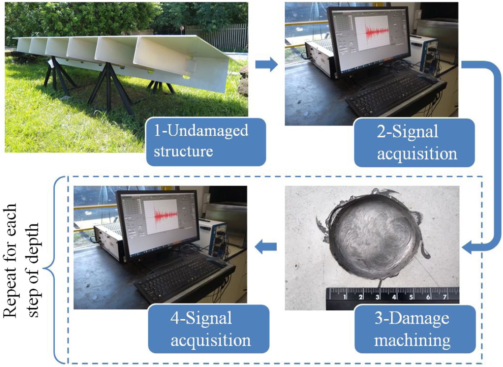
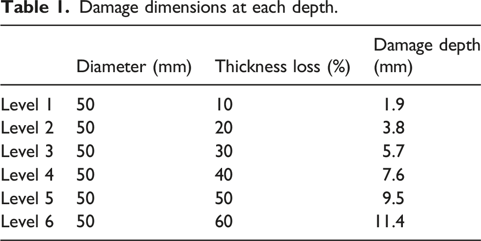
A panel was built to mimic a region of the storage tank of an FPSO called the longitudinal bulkhead, which is positioned perpendicularly to the bottom of the tank. In Figure 1(a) and (b), the design of the specimen used in the experimental tests is presented. All components that compose the specimen were made of ASTM A36 carbon steel and welded together. The specimen consists of the union of the main plate 6 m long, 2.5 m wide and 19.05 mm thick; six transversal profiles with dimensions of 2.5 m in length, 0.4 m in height and 12 mm in thickness, with distances between them of 0.9 m; one longitudinal reinforcement 6 m long, 0.6 m high and 15.88 mm thick, positioned at a distance of 0.85 m from one of the ends of the main plate. The dimensions and geometries are similar to those used in real FPSO storage tank structures. The panel was outside exposed to the weather conditions, remaining unprotected during the whole test; upper left part of Figure 2.

Figure 1.

Experimental setup from the specimen, transducer and damage. (a) Sensors placement, (b) damage placement and (c) schematic drawing of the structure with the identification and position of the transducers and the position of the damage.

Figure 2.

Flowchart of the data acquisition process of the pristine and damaged structure.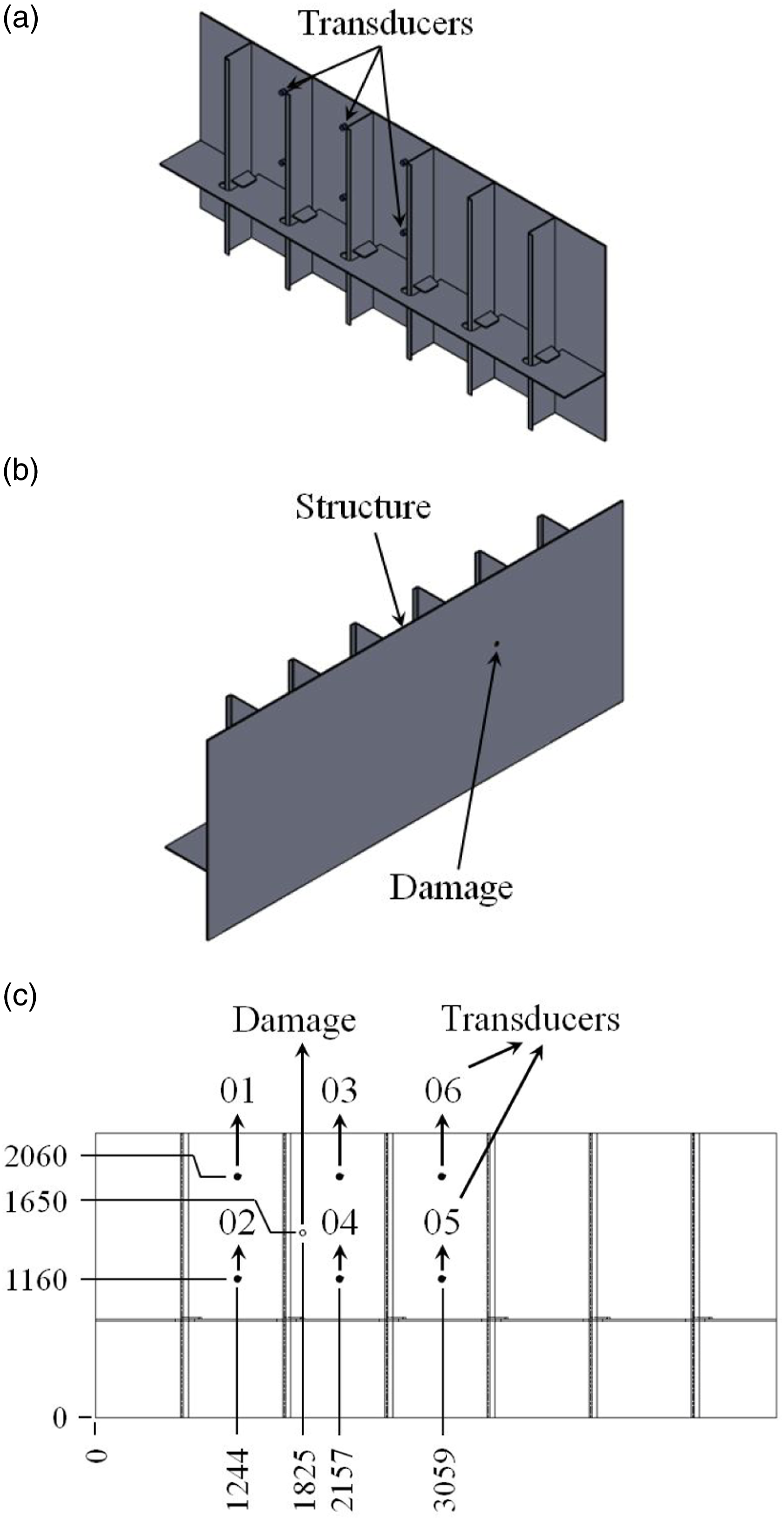

An array of piezoelectric sensors was permanently installed subsequently to the construction of the specimen. Figure 1(a) and (c) present through schematic drawings the experimental configuration of the instrumented specimen, with the arrangement composed of six piezoelectric transducers distributed on the surface of the main plate. For the positioning of the transducers, alignment at right angles was considered both vertically and horizontally, whose dimensions of the positions of each transducer are indicated in the schematic drawing of Figure 1(c). As can be seen in Figure 1, the transducer positioning was meant to be symmetrical in relation to the structural feature; it is outside of the scope of this work to perform transducer positioning optimization, as studies on that topic already exist in the literature.²⁹

A guided wave SH₀ mode was used to interrogate the structure. It is a non-dispersive mode that has a group velocity of 3260 m/s. The sensor used was developed by Ref. [30] – refer to this publication for more information. We adapted the sensors by adding a metallic housing, which provides protection against adverse weather conditions. A connector has been provided in the enclosure for the connection of the acquisition equipment and a cover for its protection. We used an epoxy adhesive for coupling the transducers with the surface of the main plate.

The pristine database is formed by a distinct dataset for each pair of sensors. We acquire signals to at least cover temperatures between 5^o C and 39^o C. This approach leads to an unequal number of signals for each sensor pair due to weather conditions, because we started collecting from sensor 1. Emissions performed by transducers from 1 to 6 have 73, 202, 250, 212, 216 and 220 signals, respectively. Subsequently, damage to the panel was reproduced in six levels of depth to represent damage by corrosion. A guided wave test was made for each damage level within this temperature range. Figure 2 shows a schematic workflow of this step.

The defect dimensions at each depth stage are shown in Table 1. The defect is a circular notch machined with a diameter of 50 mm in six steps of depth, starting with 1.9 mm of depth (10% loss of thickness) until 11.4 mm of depth (60% of thickness loss). The definition of the dimensions and geometry of the defect was based on the recommendations of the Pipeline Operators Forum³¹ for surveying Probability of Detection in the case of alveolar and generalized corrosion.

Table 1.

Damage dimensions at each depth.

	Diameter (mm)	Thickness loss (%)	Damage depth (mm)
Level 1	50	10	1.9
Level 2	50	20	3.8
Level 3	50	30	5.7
Level 4	50	40	7.6
Level 5	50	50	9.5
Level 6	50	60	11.4

The waveform considered for the measurements was a tone burst type with a central frequency of 45kHz and the number of cycles equal to five. This was selected based on the best response of the transducer and, empirically, in terms of characteristics of the resulting signals. The sampling frequency used in the tests was 1 MHz. We use the mean value of 50 measurements to reduce the variance caused by the white noise in the recorded data. All transducers were excited using a National Instruments PXIe-5451 arbitrary waveform generator and a Krohn-Hite 7500 amplifier source. The signals were acquired using an oscilloscope PXI-5105 from National Instruments. All signals were pre-processed with a band-pass Butterworth filter with cutoff frequencies of 11.25 kHz and 67.5 kHz and windowed in order to remove cross-talk.

In order to label the data to feed our outlier detector model, we defined a nomenclature formed by letters and numbers for each pair of sensors. For example, the pair of sensors designated as e1r2 is composed of transducer 1 as a signal emitter and transducer 2 as a signal receiver along with others. Among the thirty possible combinations of pairs of sensors in the arrangement, composed of six sensors, we selected the following pairs of emitting and receiving sensors: e1r2, e2r3, e4r3, e4r1, e5r1 and e6r2. As shown in Figure 1(c), depending on the pair of sensors, there may be one or two welded structural elements between the sensors and the damage, and, in some cases, both the structural element and the damage are not located between the sensors. In addition, depending on the sensor pair, the damage could be closer to the emitter sensor or closer to the receiver sensor.

Application of the data-driven algorithm

The proposed method uses the ICA algorithm to reduce the dimension of the data from the GW test. The reduced data was used to identify the component referring to the damage in an automatic way using an outlier detector. The first dataset is related to pristine conditions and the second dataset is related to the undamaged raw data plus one signal added, in a random position. The components of the two datasets were related to each other through the maximum value of the cross-correlation. Thus, the component of the defect will tend not to be linked because it must have less similarity with the components of the first set. Finally, this process was repeated several times to calculate the accuracy and errors (Type I and II errors as shown in Table 2) of damage detection and to calculate the signal-to-noise ratio (SNR) of the outliers components to quantify the damage. A schematic flowchart of the process can be seen in Figure 3. The algorithm developed in this study was implemented using Python programming language, which provides all the tools needed.

Table 2.

Type of errors.

	Negative	Positive
False	Accuracy	Type I
True	Type II	Accuracy

Figure 3.

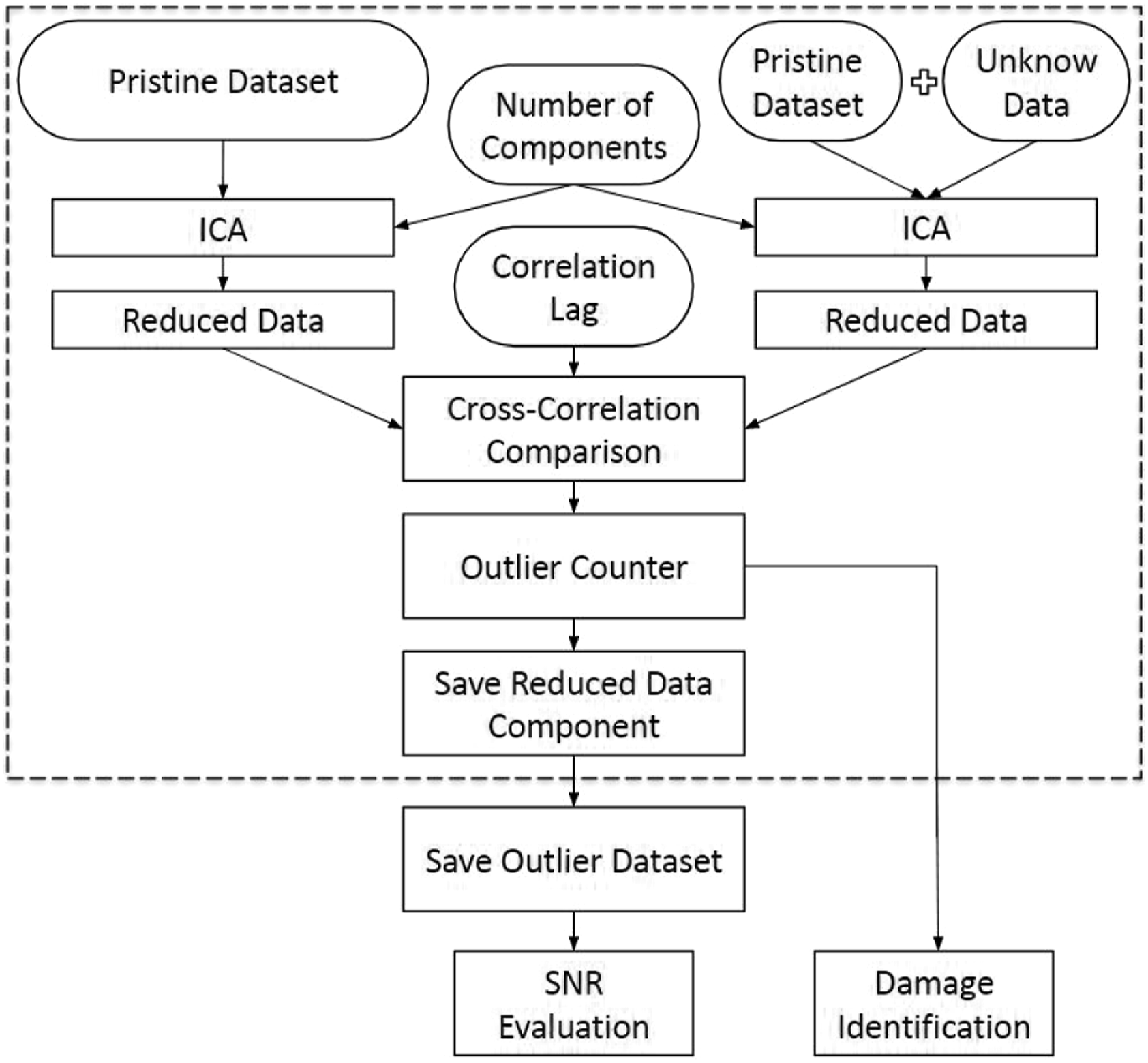
Flowchart of the data-driven algorithm application process for damage detection and quantification.

In order to quantify the error rates, we follow the confusion matrix showed in Table 2. Accuracy is considered to be when there is a defect and our method detects it and when there is no defect and our method does not detect this; false positives are called Type I-error and are when our method missed to classify one existing defect; true negatives are Type II-error and occur when our method classifies one defect that does not exist. In a real world application case, there is no information about the structure integrity, it means, the added signal is from an unknown condition, it can represent some damage or not. However, in laboratory tests, it is possible to identify if the signal came from a pristine condition or not.

The application process of the data-driven algorithm is divided into two parts: the first part is represented by the steps that are inside the rectangle of dashed lines of the flowchart (Figure 3); the second part is represented by the steps that are outside the rectangle of dashed lines of the flowchart. The first part of the process must be repeated N before the evaluation of the second part.

The first part aims to compare two different datasets: one composed of the pristine structure condition; the other is the same pristine structure condition plus one unknown signal. To build the datasets, we proceed as follows: we withdraw random samples (using a uniform law and without replacement) from a data pool and stack them to construct a data matrix. To keep the same methodology, the unknown data (plus one signal) is added and randomly insert in the data matrix. The number of baseline signals used in the tests was based on the number of experimental signals collected for each emitting transducer. Thus, the number of 100 random baseline signals was defined, except for sensor combinations where transducer 01 is the actuator because it has a smaller number of experimental baseline signals collected, in this case, we considered 70 random baseline signals. Figure 4 shows an example of the data matrix from the data pool from pair of sensors e1r2 considering 70 baseline signals. Figure 4 shows also the variation of temperature.

Figure 4.

Distance versus baseline and the measured temperature. (a) Distance versus baseline signal for the pair e1r2 and the measured temperature and (b) distance versus baseline plus defect signal for the pair e1r2 and the measured temperature.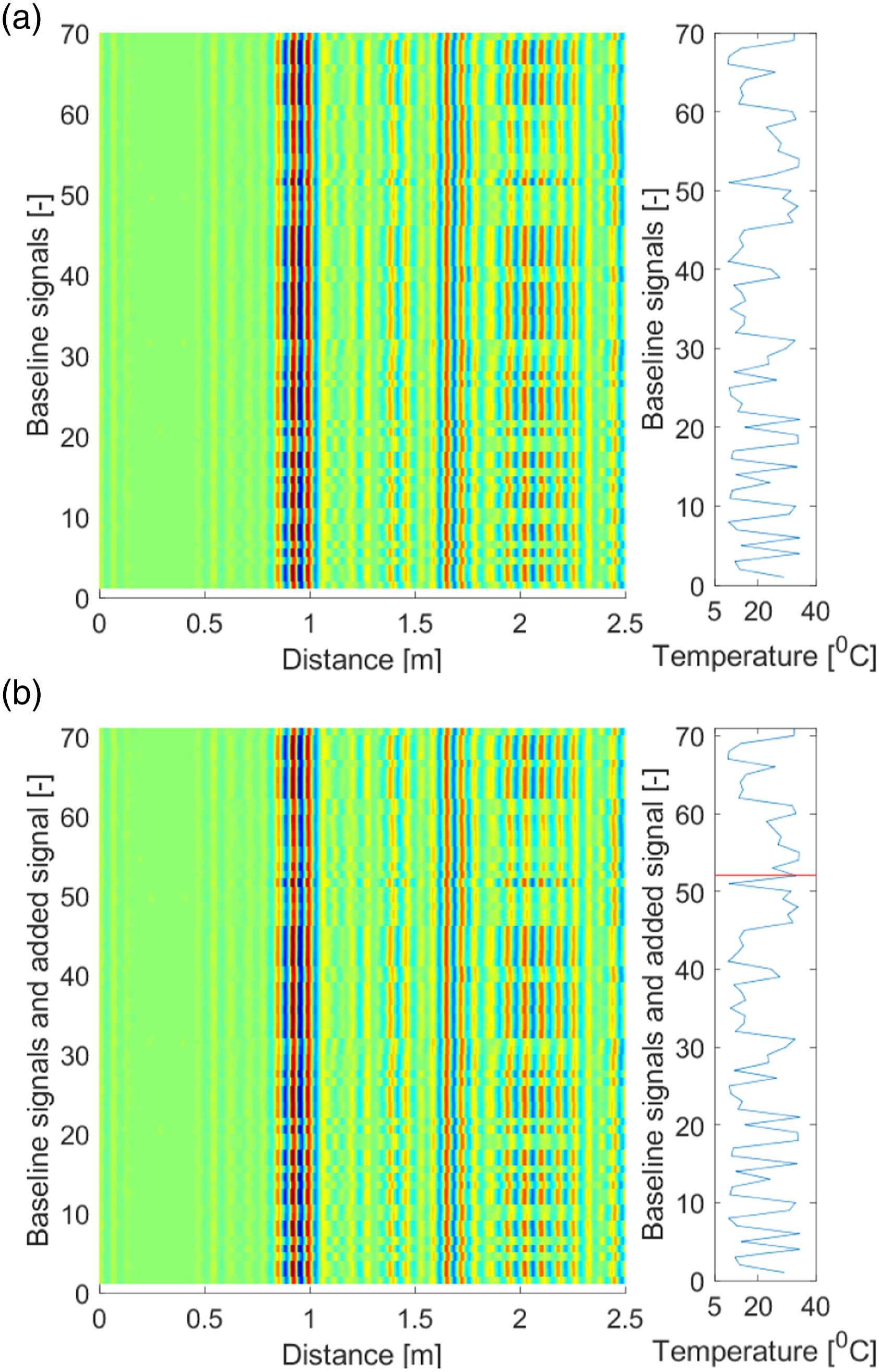

The ICA try to minimize the degree of statistical dependence of the components, such as mutual information,³² estimation of maximum likelihood and maximization of non-Gaussianity (kurtosis or negentropy).³³ Furthermore, several implementations of the ICA algorithm are presented in the literature.^34,35 ICA despite being efficient, had a high computational cost.³⁶ For this reason, several authors looked for new alternatives to improve, accelerate or optimize this process.^37–39 We expect that when a ‘new statistic information’, it means, a defect is added to the dataset new ICA weights components should be created. On the other hand, if there is no defect there is no ‘new statistic information’ and no needed for new ICA weights components.

In order to improve the visualization of the method, we added the signal corresponding to the damage level 6 among the other baseline signals (red line in Figure 4(b)). Figure 5 shows the result of applying the ICA algorithm to these signals, considering 10 independent components. In Figure 5(a), the result for the first set of components is presented. Figure 5(b) presents the result for the second set of components.

Figure 5.

Weights components of the pair e1r2. (a) Baseline weights components of the pair e1r2 and (b) Baseline plus defect weights components of the pair e1r2.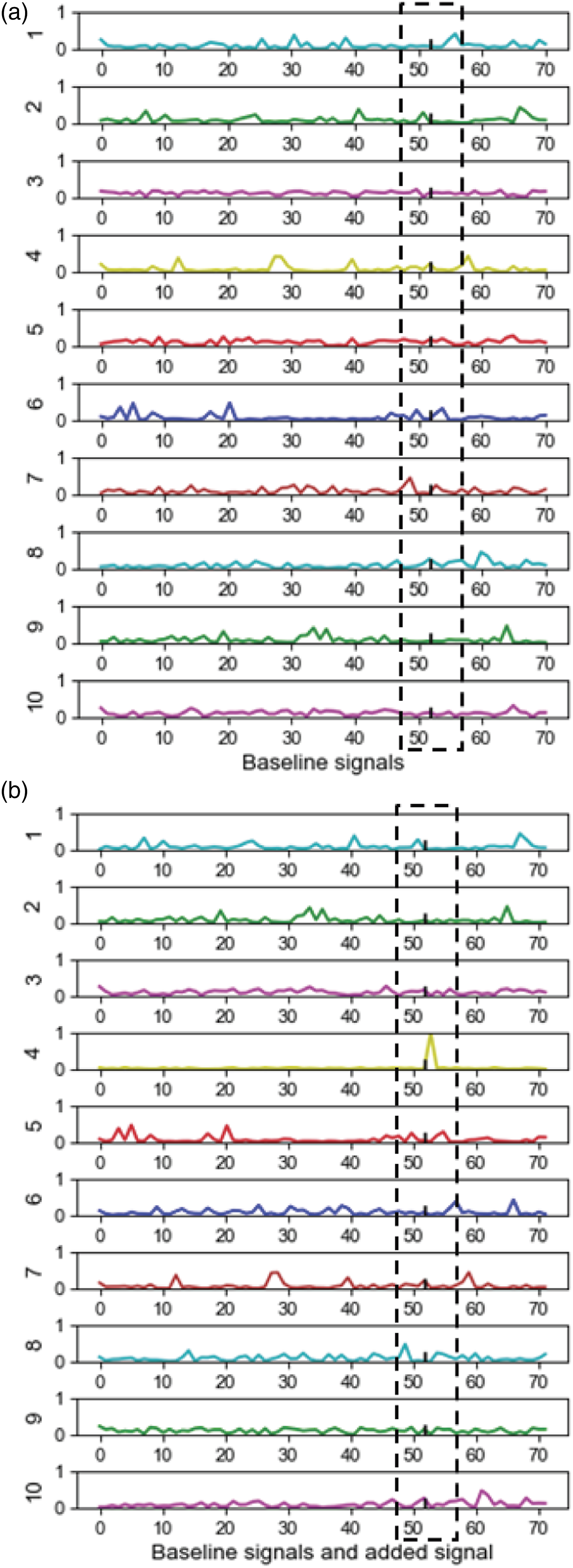

Following the flowchart of Figure 3, we evaluated the cross-correlation between all ICA weights on the first dataset and the second dataset (they are presented in Figure 5(b)). In this case, it can be seen that component 4 has less similarity than the other components and it is assumed as the component related to the damage. The search for the maximum value of each cross-correlation was carried out from three lag intervals called Case 1 (entire lag vector), Case 2 (lag sample range was restricted to ±10) and Case 3 (lag sample range was restricted to ±2). This step tries to minimize the errors choosing only the most similar component. Then, a matrix is generated relating (using the maximum of the cross-correlation) the components of the first set of components with the components of the second set.

After completing the first part of the process, the accuracy, Type I-error and Type II-error for damage identification are quantified through the number of random realizations performed. Finally, the SNR is calculated only for the components of the weights of the second set of components that obtained the lowest similarity. To perform the SNR calculation, the maximum value divided by the average value of the vector is considered.

To analyze the influence of the number of ICA components, tests were carried out varying this number from 10 to 40 in intervals of 5 independent components. From the values of the peak amplitude in the component that has the maximum value at the position where the defect signal was added. It is intended to analyze the number of independent components necessary to detect and quantify the damage at all depth stages.

Figure 6 shows an example of the result of applying the data-driven algorithm on the e2r3 pair of sensors considering Case 3. Figure 6(a) shows the results of accuracy for the undamaged and damaged structure depending on the number of random realizations. On the defect depth axis, the accuracy for the value 0 (in the axis Defect depth) are related to the undamaged structure and the other accuracy are related to the damaged structure with thickness losses between 10% and 60%. Figure 6(b) shows the results of the Type I-error rates, which are related to the damaged structure, according to the number of random realizations. Finally, in Figure 6(c), the results of the Type II-error rates are presented, which are related to the undamaged structure, according to the number of random realizations.

Figure 6.

Influence of the number of random realizations in the accuracy, type I and II errors in the e2r3 sensor pair for Case 3. (a) Accuracy, (b) Type I-error and (c) Type II-error.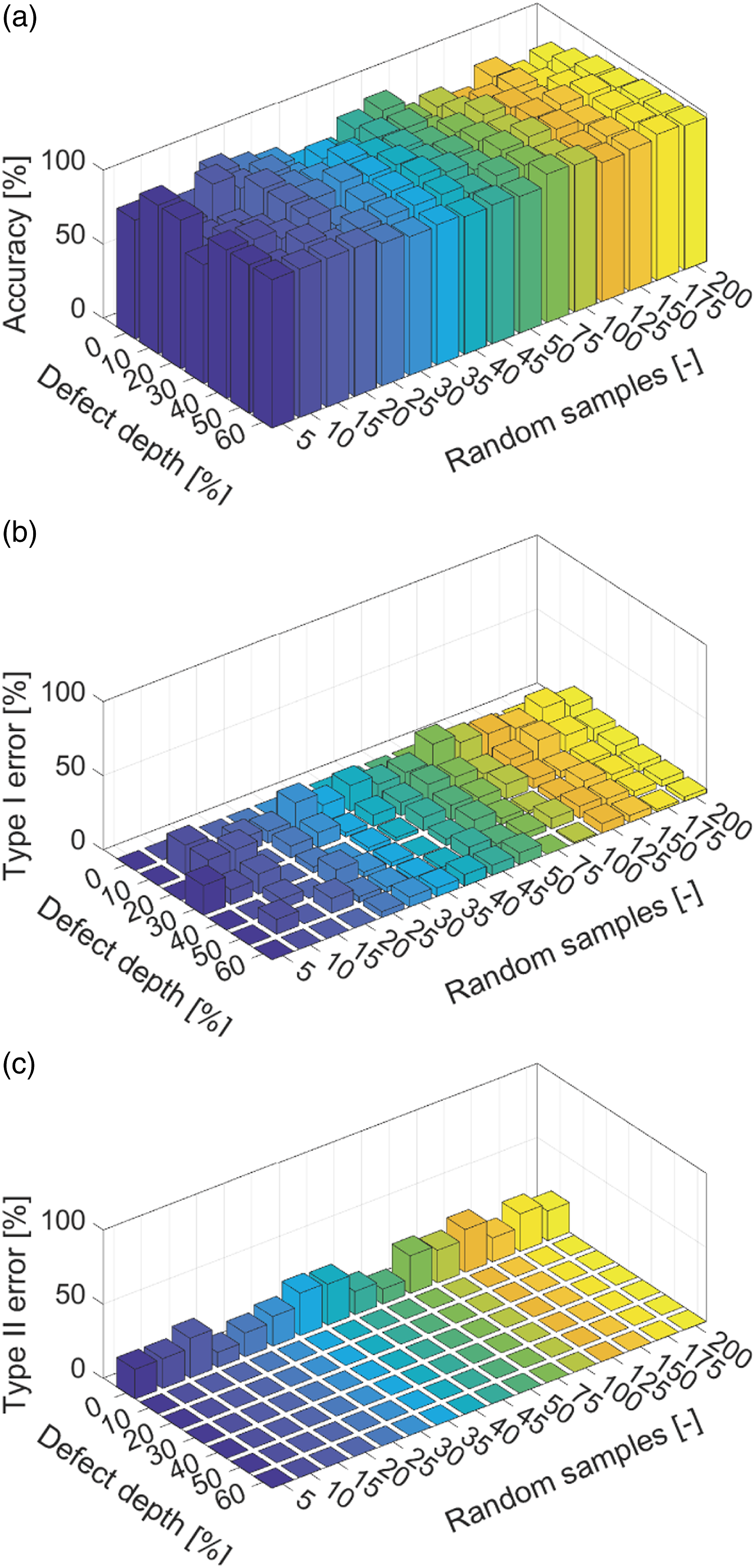

In order to analyze the influence of the number of random realizations and the pair of sensors, the mean and the standard deviation of the accuracy (defect depth axis) were used, considering the undamaged and damaged structure at all depth stages, depending on the number of random realizations. As for the Type I-error, the mean and the variance of the error rates of the defect depth axis were used as well, considering only the damaged structure at all depth stages, according to the number of random realizations. Finally, for the Type II-error, we considered the value of the error rate of the defect depth axis, considering only the pristine structure, according to the number of random realizations.

Results

Damage detection results

Influence of the number of independent component analysis component

Figure 7 shows the influence of the size of reduced dimension in the amplitude of the component. It is possible to observe that the pairs of sensors have different behaviours regarding the peak amplitude value that has the maximum value at the position where the unknown signal was added. The number of 10 components is represented in blue and a circle, 15 components in orange and an upward triangle, 20 components in green and a square, 25 components in red and a diamond, 30 components in purple and a triangle to the left, 35 components in grey colour and a triangle to the right and 40 components in brown colour and a star.

Figure 7.

Influence of the number of ICA components on sensor pairs: 10 components are represented in blue colour and a circle, 15 components in orange colour and an upward triangle, 20 components in green colour and a square, 25 components in red colour and a diamond, 30 purple components and a triangle to the left, 35 grey components and a triangle to the right and 40 brown components and a star. (a) Number of components influence for e1r2, (b) number of components influence for e2r3, (c) number of components influence for e4r3, (d) number of components influence for e4r1, (e) number of components influence for e5r1 and (f) number of components influence for e6r2.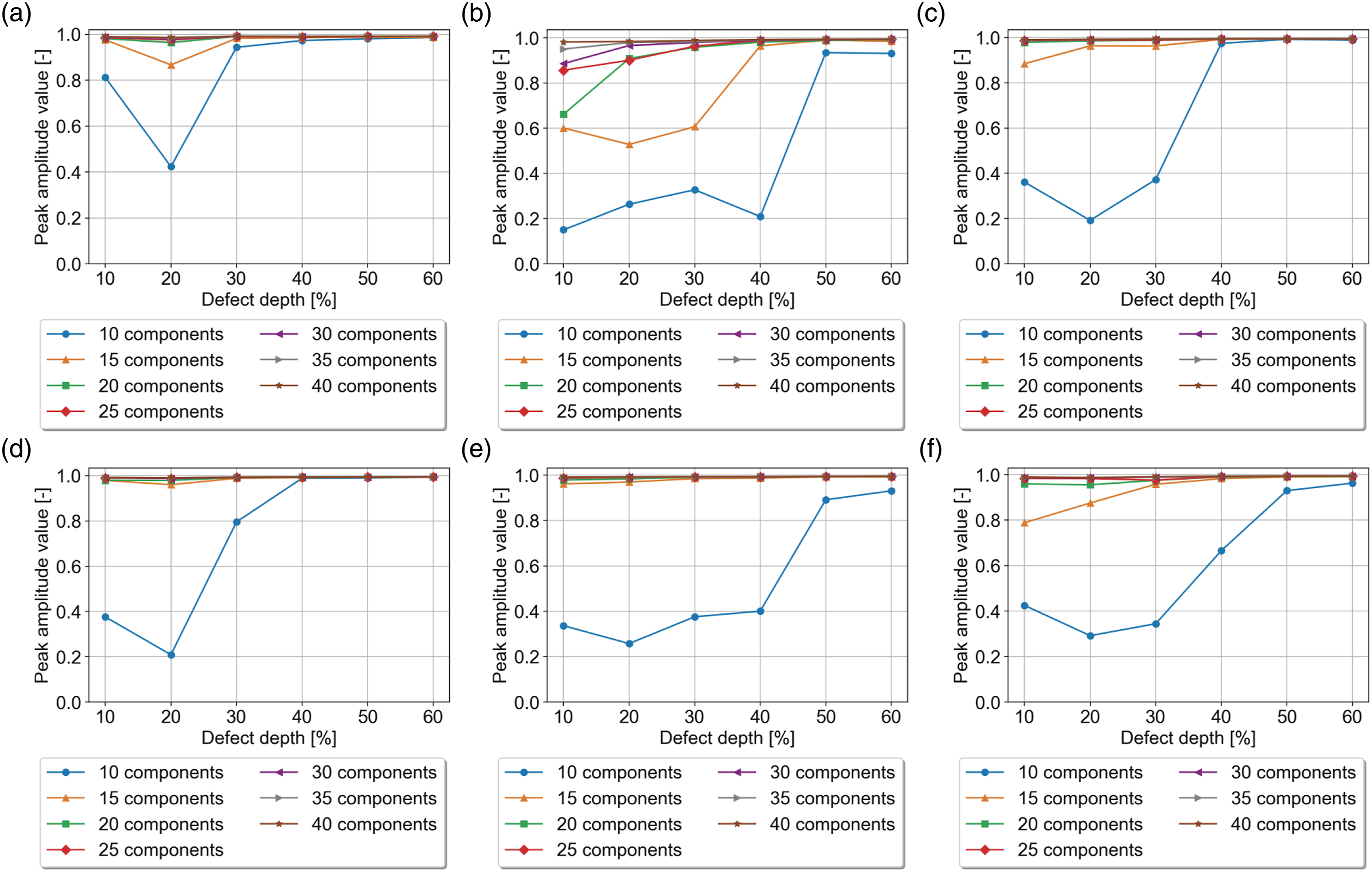

Figure 7 shows the influence of the number of independent components for the sensor pairs e1r2, e2r3, e4r3, e4r1, e5r1 and e6r2. In the performed tests with different numbers of independent components, it was observed that it was not possible to detect damage using the number of components with peak amplitude values close to or below 0.6. The best results obtained for both, the damage detection rate and the damage severity quantification, were with the first number of components. Considering the increasing order of the number of components tested, which obtained peak amplitude values from approximately 0.8. The results show that as the number of components increases, the peak amplitude values increase as well, especially in less severe damage. For more severe damage, stabilization of the increase in peak amplitude values occurs with smaller numbers of components. For sensor pairs e1r2, e4r3, e4r1, e5r1 and e6r2, it is observed that with 15 independent components, the first peak amplitude values close to or above 0.8 are obtained considering all depth stages. As for the pair of e2r3 sensors, it is observed that with 25 independent components, the first peak amplitude values above 0.8 are obtained considering all depth stages.

Influence of the number of random realization

Figure 8 show the results of the influence of the number of random realizations in the accuracy, Type I and II errors for the sensor pairs e5r1. Cases 1, 2 and 3, are presented with the mean value represented by solid lines and shaded regions represents one standard deviation. The green colour stands for Case 1, the blue colour stands for Case 2 and the red colour stands for Case 3. We are presenting them as a representative behaviour of all pair sensor data.

Figure 8.

Influence of the number of random realizations in the accuracy, Type I and II errors in the e5r1 sensor pair. Cases 1, 2 and 3 are represented by solid lines and shaded regions of green, blue and red colours, respectively. For accuracy, Type I and II errors, solid lines represent rate averages and shaded regions represent one standard deviation. (a) Accuracy, (b) Type I-error and (c) Type II-error.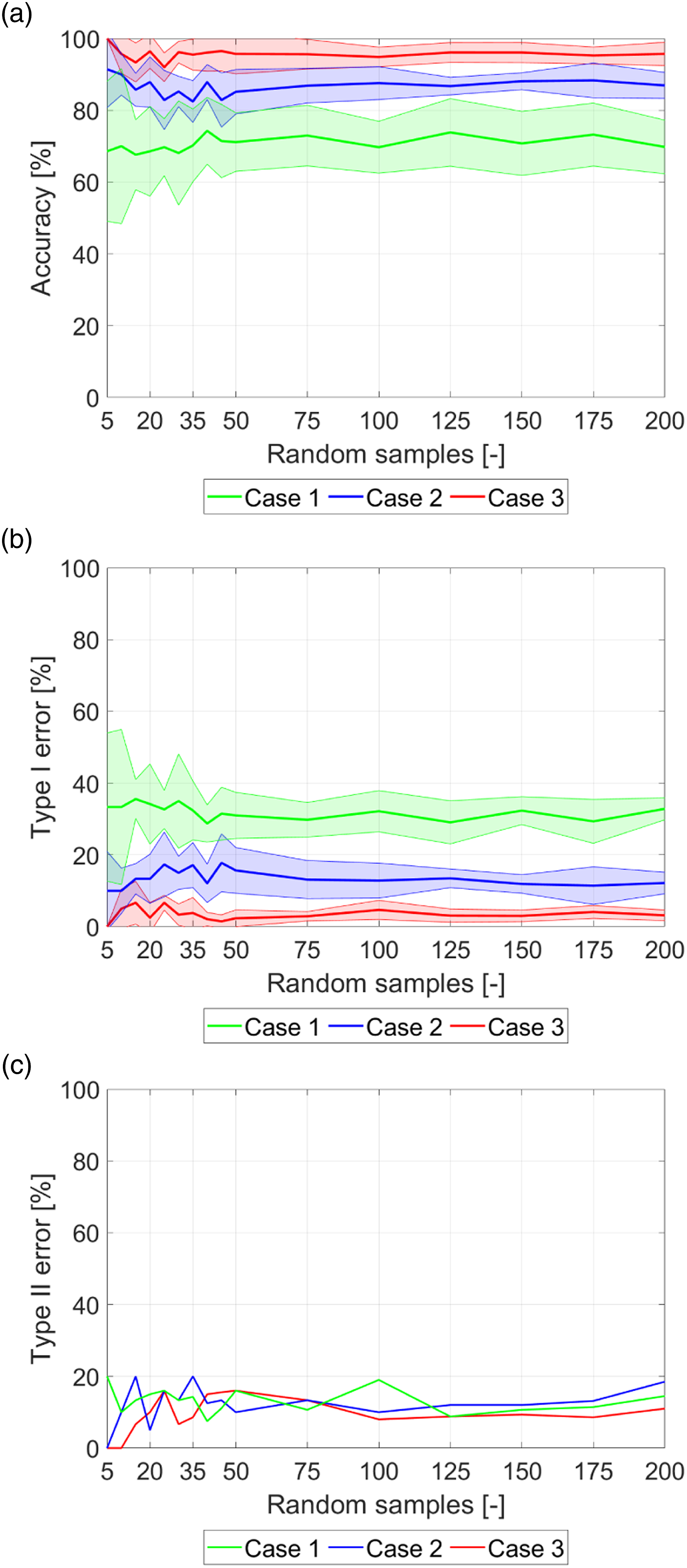

Figure 8(a) shows the accuracy of the model. We can observe that as the lag interval is restricted, the average values of the accuracy rates according to the number of random realizations increase. Furthermore, it is possible to observe in all pairs of sensors that the variance decreases as the lag interval is restricted. Thus, it indicates that the mean damage detection accuracy is more stable. We would like to stress that small defects show a lower accuracy, on the contrary, larger defects present higher accuracy, as shown in Figure 6.

Figure 8(b) shows the Type I-error rates. We can draw similar conclusions to those made for accuracy. Nevertheless, the error rates decrease with the lag distance. We emphasize that the reduction in variance is due to the central limit theorem. It states that the variance should reduce when the number of samples increases by an inverse of a square root. The errors, on the contrary, are a function of the algorithm proposed and not a function of the number of random samples, which is why did not reduce. Figure 8(c) shows the Type II-error rates. We see almost no influence of the lag distance or random samples in the model result.

Figure 9 shows the influence of the number of realizations in the accuracy, Type I and II errors for lag case 3 in all sensor pairs. Sensor pairs e1r2, e2r3, e4r3, e4r1, e5r1 and e6r2 are represented by solid lines of red, blue, cyan, green, magenta and black colours, respectively (solid lines represent the averages).

Figure 9.

Influence of the number of random realizations in the accuracy, Type I and II errors for case 3 in all sensor pairs. Sensor pairs e1r2, e2r3, e4r3, e4r1, e5r1 and e6r2 are represented by solid lines of red, blue, cyan, green, magenta and black colours, respectively. For accuracy, Type I and II errors, solid lines represent rate averages. (a) Accuracy, (b) Type I-error and (c) Type II-error.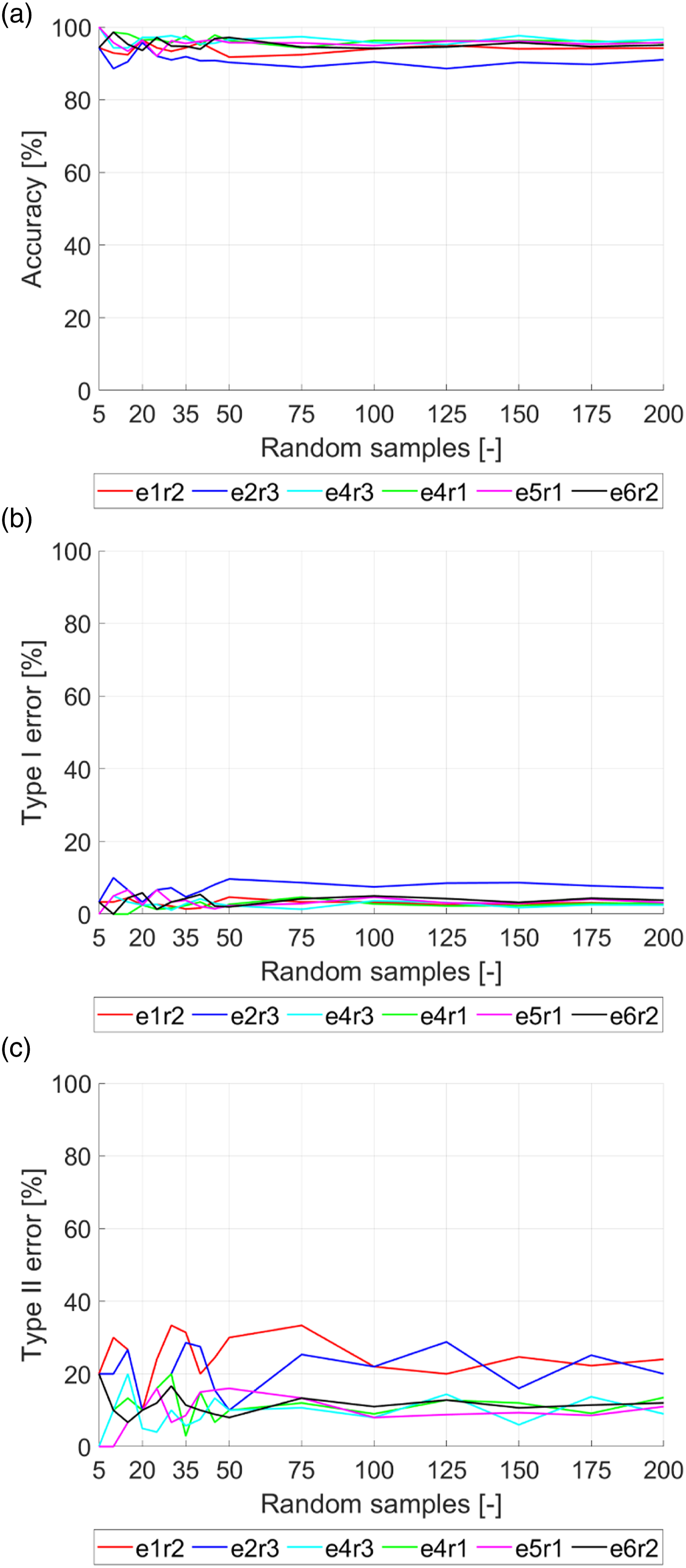

In Figure 9(a) and (b), the behaviour of the sensor pairs seems to be similar. They become more stable when the number of samples is increased. However, we note that some pairs perform a less accurate prediction. Clearly, these same pairs have a higher Type I-error (around 15% in the maximum value, e2r3, and 5% for the others). Regarding the Type II-error (Figure 9(c)), we see a less conscious data. There are strong variations in the error rate, especially for the pairs e1r2 and e2r3, they present, also, the large prediction error. The other pair sensors predict errors below 20%.

Of the many variables that can influence the results, some are unfortunately impossible to decouple. Handmade sensors produce variations in the responses of each pair. The condition of ambient noise and temperature variations, high for guided wave applications and complexity of the structure. The path taken by the wave, if there is direct or indirect interaction with the defect. Even with all these variables, the method is robust with a 95% defect identification rate.

Damage quantification results

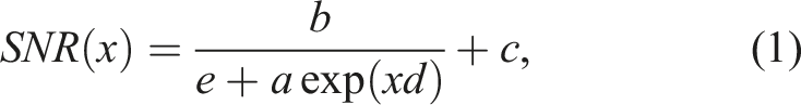
Figure 10 shows the SNRs versus damage for all depth stages for the sensor pairs e1r2, e2r3, e4r3, e4r1, e5r1 and e6r2. The SNRs are from Case 3 and 200 random realizations. Observing Figure 10(a), a sigmoidal relationship between the SNR outliers and the damage in the structure can be seen. This relation can be used to estimate the severity of the damage in the structure. Nevertheless, it can be seen the clear dependence of the sensor pair on the sensitivity to the defect. Unlike the results obtained for the identification, where the variables, such as the wave path (sensor pair) had little influence here and it exerts a strong influence.

Figure 10.

SNRs versus damage for Case 3 with 200 samples. The solid line represents a regression using a sigmoid function on the outliers and the dashed lines represent the 95% confidence limits.(a) SNRs for sensor pair e1r2 for Case 3 with 200 samples, (b) SNRs for sensor pair e2r3 for Case 3 with 200 samples, (c) SNRs for sensor pair e4r3 for Case 3 with 200 samples, (d) SNRs for sensor pair e4r1 for Case 3 with 200 samples, (e) SNRs for sensor pair e5r1 for Case 3 with 200 samples and (f) SNRs for sensor pair e6r2 for Case 3 with 200 samples.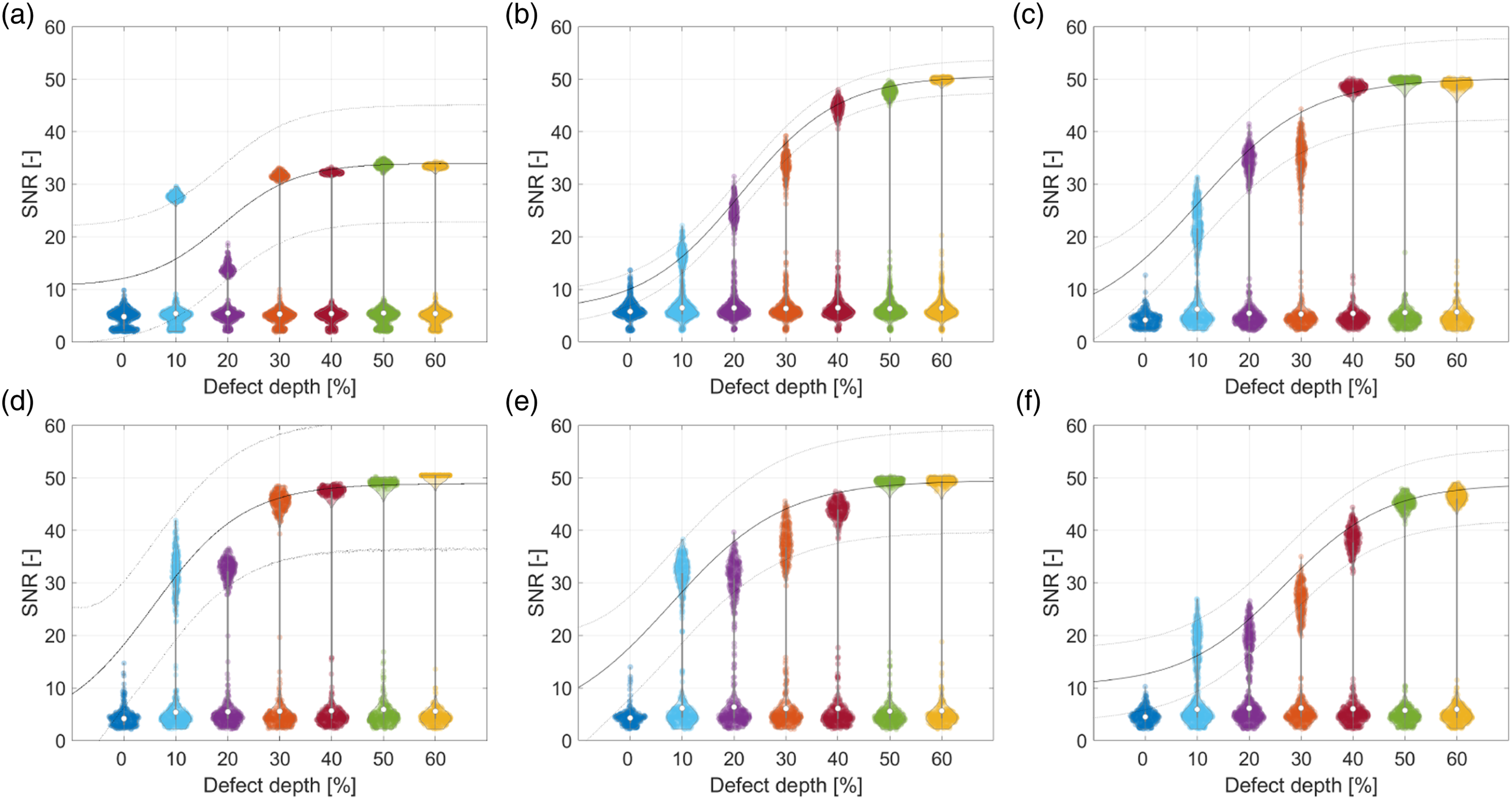

It is possible to draw some relations between the wave path and the results presented in Figure 10. The SNR values are related to the paths shown in Figure 1(c). The reason for the better quantification results presented in the e2r3, e5r1 and e6r2 pairs is possibly due to the direct passage of the guided wave in the damage. In addition, to the influence of paths and welded structural elements, the damage itself produces mode conversion. Thus, more energy is lost, making quantification even more challenge. The e4r3 sensor pair (Figure 10(c)) does not have the direct passage of the guided wave in the damage. However, the quantification result can be justified by the absence of structural elements welded between the sensors and between the sensor pair and the damage. The ‘better quantification’ means a reduced slope in the sigmoid curve. As for the e1r2 (Figure 11(c)) sensor pair, we can justify the unsatisfactory result of the quantification because it does not have the direct passage of the guided wave in the damage and also because of the presence of a structural element welded between the sensor pair and the damage.

Figure 11.

Influence of the number of random realizations on the SNRs of the undamaged and damaged structure at all depth stages for the e1r2 sensor pair for Cases 1, 2 and 3 with 200 samples. The solid line represents a regression using a sigmoid function on the outliers and the dashed lines represent the 95% confidence limits. (a) SNRs for Case 1 with 200 samples, (b) SNRs for Case 2 with 200 samples and (c) SNRs for Case 3 with 200 samples.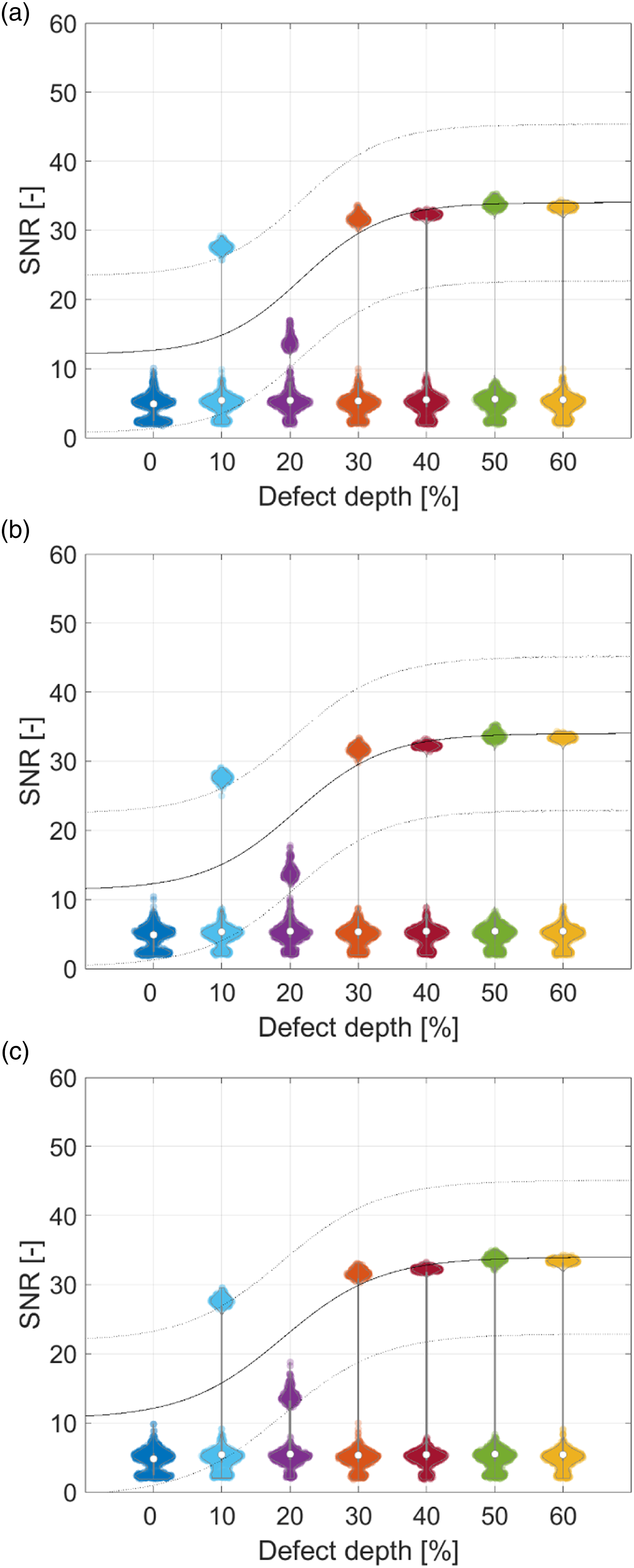

A sigmoid curve was used to fit the data from the various sensor pairs. It is presented in equation (1)

S N R (x) = \frac{b}{e + a \exp (x d)} + c,

(1)

where x is the defect size in % thickness loss and a, b, c, d and e are constants to be fitted. The fit of the sigmoidal curve and the confidence limit curves in the outliers will allow estimating the damage depth. In the Table 3, the values obtained in the regression for all sensor pairs are shown. In Figure 10, the regression using the sigmoid function on outliers is represented by the solid line and the 95% confidence limits are represented by the dashed lines.

Table 3.

Values obtained in the regression using the sigmoid function on the outliers for 200 random realizations for Case 3.

	e1r2	e2r3	e4r3	e4r1	e5r1	e6r2
a	−2.5 × 10⁴	7369	8.29	6.01	9.52	−4726
b	−4.1 × 10⁴	34,690	148.4	149.9	217.2	−1.1 × 10⁴
c	10.57	5.82	2.99	1.998	2.45	10.36
d	−1.40	−1.05	−0.93	−1.13	−0.92	−1.02
e	−1787	773.5	3.147	3.19	4.61	−298.5
r ²	0.71	0.99	0.92	0.83	0.86	0.94

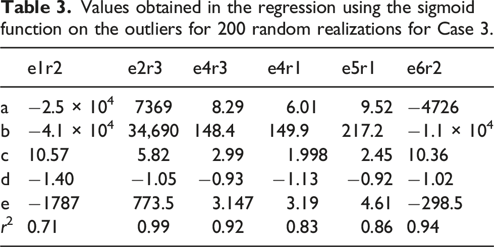
According to the results presented in Figure 10 for different pairs of sensors, we can observe that the SNR is relatively sensitive for estimating the depth of damage with smaller depths, allowing us to estimate the depth of damage in the early stages. As for damages with greater depths, the SNR is less sensitive to estimating the depth. The lower sensitivity for damage with greater depths is a characteristic of the model developed itself. Finally, because the developed method does not perform damage localization, it is not possible to define the best pair of sensors. However, we can use the algorithm developed by Menin et al.,⁴⁰ for example, which performs the localization of damage through a classical image. From the damage location, we will possibly be able to choose the best pair of sensors to perform the damage quantification through the SNR.

Figure 11 shows the results of Cases 1, 2 and 3 for the e1r2 sensor pair. It shows that the damage quantification is lightly influenced by the lag interval. It was found that the amount of outliers increases in the same proportion as the accuracy increases, in the e1r2 pair of sensors for Cases 1, 2 and 3 for 200 random realizations. In the similar way, it was verified that the amount non-outliers related to the lowest values decrease in the same proportion that the Type I-error rate decreases in the e1r2 pair of sensors. For the other pairs of sensors, the same behaviour described for the pair of sensors e1r2 was observed.

Conclusion

In this work, we proposed a method for detecting and quantifying damage related to thickness reduction in complex and difficult-to-access structures, using the outlier detector algorithm in a guided wave SHM system, permanently installed in a structure. Furthermore, this study complements the work of Menin et al.,⁴⁰ who had developed a technique for locating damage in complex structures using the same structure and the same experimental data.

A study varying the number of ICA independent components had shown that the greater the number of independent components, the more stable are the peak values of the amplitude in the component of the weights at the position of the defect signal. In addition, we showed that components related to more severe damage tend to have higher values and a faster stabilization for the peak amplitude, and, for less severe damage a greater number of components is needed in order to obtain the same peak values. The best results obtained for the detection and quantification of the damage were with the first number of independent components, considering the increasing order of the number of components tested, which obtained peak amplitude values from approximately 0.8.

As for the detection of damage, the variation of the lag interval for the search for the maximum value of the cross-correlation showed that from the smallest lag interval tested, the highest accuracy rates and the lowest Types I and II-error rates were obtained. The best result was achieved using the lag Case 3, with a lag range of −2 to 2, average accuracy rates above 90%, Type I-error rates below 10% and Type II-error rates below 35%. The smaller the lag interval for the search for the maximum value of the cross-correlation and the greater the number of random realizations, the more stable are the averages of the accuracy and Types I and II-error rates. In addition, we reinforce that those rates tends to be majored by the lower boundary, once small defects have less accuracy, as noted by inspection in Figure 6.

Using the outliers SNRs values of the undamaged and damaged structure, it was possible to identify if the structure is intact and to quantify the damage at all depth stages in the e2r3, e4r3, e5r1 and e6r2 sensor pairs. The adjustment of a sigmoidal curve through the sigmoid function in the SNRs of the outliers allowed us to quantify the damage severity more precisely. The undamaged structure always obtained the lowest values of the SNRs of the outliers. Less severe damage is indicated with lower outliers SNR values and more severe damage with higher values. The results showed that the quantification of damage is lightly influenced by the lag interval for the search for the maximum value of the cross-correlation.

Finally, for both, detection and quantification of damage, the method proved to be independent of temperature and other environmental conditions. The pre-process used in the GW data were very simple one without the need for complex processing, such as temperature compensation. In future works, we intend to locate the damage through the ICA components related to the guided wave signals.

Footnotes

Declaration of conflicting interests

The author(s) declared no potential conflicts of interest with respect to the research, authorship, and/or publication of this article.

Funding

The author(s) disclosed receipt of the following financial support for the research, authorship, and/or publication of this article: This work was supported by the Agência Nacional de Petróleo, Gás Natural e Biocombustíveis.

ORCID iDs

Lúcio de Abreu Corrêa

Paulo Dambros Menin

References

Allahyarzadeh-Bidgoli

Dezan

Salviano

, et al. Lifetime sensitivity analysis of fpso operating parameters on energy consumption and overall oil production in a pre-salt oil field. Chem Eng Commun 2020; 207(11): 1483–1507.

Leal

GLN

Naked

. A fuzzy logic-possibilistic methodology to analyze the main corrosion damages mechanisms in pipes and equipment installed in an oil and gas platform. Int J Sci Qual Anal 2019; 5(1): 15.

Ozguc

. Conversion of an oil tanker into fpso in gulf of mexico: strength and fatigue assessment. Ships and Offshore Structures 2020; 16: 1–19.

Ozguc

. Fatigue assessment of fpso hull side shell longitudinals using component stochastic and full spectral method. Appl Ocean Res 2020; 101: 102289.

Hageman

van der Meulen

Rouhan

, et al. Quantifying uncertainties for risk-based inspection planning using in-service hull structure monitoring of fpso hulls. Mar Structures 2022; 81: 103100.

Huan

Chen

. A practical omni-directional sh wave transducer for structural health monitoring based on two thickness-poled piezoelectric half-rings. Ultrasonics 2019; 94: 342–349.

Huan

. A baseline-free sh wave sparse array system for structural health monitoring. Smart Mater Structures 2019; 28(10): 105010.

Abbas

Shafiee

. Structural health monitoring (shm) and determination of surface defects in large metallic structures using ultrasonic guided waves. Sensors 2018; 18(11): 3958.

Clarke

. Guided Wave Health Monitoring of Complex Structures. PhD Thesis. Department of Mechanical Engineering, Imperial College London, 2009.

10.

Tabjula

Kanakambaran

Kalyani

, et al. Outlier analysis for defect detection using sparse sampling in guided wave structural health monitoring. Struct Control Health Monit 2021; 28(3): e2690.

11.

Monnier

Hebaz

. Guided wave topological energy method for quantitative evaluation of corrosion in metal plates and tubes. In: Forum Acusticum, Lyon, France, 12 2022, pp. 1855–1862.

12.

Giroto

Viera

MAA

Junior

, et al. Development of a piezoelectric transducer coupling system for structural health monitoring applications. In: 7th International Engineering, Sciences and Technology Conference (IESTEC), Panama, Panama, 09-11 October 2019. IEEE, pp. 538–543.

13.

Wang

Zhang

Shen

, et al. Defect detection in guided wave signals using nonlinear autoregressive exogenous method. Struct Health Monit 2021; 21: 1012–1030.

14.

Farrar

Worden

. Structural Health Monitoring: A Machine Learning Perspective. USA: John Wiley & Sons, 2012.

15.

Mesnil

Imperiale

Demaldent

, et al. Simulation tools for guided wave based structural health monitoring. AIP Conf Proc 2018; 1949: 050001. AIP Publishing LLC.

16.

Cawley

. Ultrasonic structural health monitoring-current applications and potential. In: IEEE International Ultrasonics Symposium (IUS), Glasgow, UK, 06-09 October 2019. IEEE, pp. 2107–2109.

17.

Goodfellow

Bengio

Courville

, et al. Deep Learning. Vol. 1. USA: MIT press Cambridge, 2016.

18.

Oliveira

. Handshape recognition using principal component analysis and convolutional neural networks applied to sign language. PhD Thesis. Dublin City University, 2018.

19.

Rautela

Senthilnath

Monaco

, et al. Delamination prediction in composite panels using unsupervised-feature learning methods with wavelet-enhanced guided wave representations. Compos Structures 2022; 291: 115579.

20.

Schnur

Goodarzi

Lugovtsova

, et al. Towards interpretable machine learning for automated damage detection based on ultrasonic guided waves. Sensors 2022; 22(1): 406.

21.

Agis

Pozo

. A frequency-based approach for the detection and classification of structural changes using t-sne. Sensors 2019; 19(23): 5097.

22.

Bosse

Weiss

Schmidt

. Supervised distributed multi-instance and unsupervised single-instance autoencoder machine learning for damage diagnostics with high-dimensional data—a hybrid approach and comparison study. Computers 2021; 10(3): 34.

23.

van Baars Buisman

Michau

Rene

, et al. Domain adaptations for guided wave shm of composites: towards fleet monitoring. In: Proceedings of the 6th European Conference of the Prognostics and Health Management Society, Vol. 6. Prognostics and Health Management Society, Online, June 28–July 2, 2021, pp. 430–438.

24.

Ahmed

Kopsaftopoulos

. Active sensing acousto-ultrasound shm via stochastic time series models. In: Health Monitoring of Structural and Biological Systems XVI, Long Beach, USA, 19 April 2022 Vol. 12048, pp. 358–366.

25.

Fang

Liu

. Imbalanced classification of fatigue crack for aluminum plates using lamb wave. In: European Workshop on Structural Health Monitoring. Springer, Palermo, Italy, 2020, pp. 161–170.

26.

Tang

, et al. Ultrasonic guided wave-based switch rail monitoring using independent component analysis. Meas Sci Technology 2018; 29(11): 115102.

27.

Anowar

Sadaoui

Selim

. Conceptual and empirical comparison of dimensionality reduction algorithms (pca, kpca, lda, mds, svd, lle, isomap, le, ica, t-sne). Computer Sci Rev 2021; 40: 100378.

28.

Dobson

Cawley

. Independent component analysis for improved defect detection in guided wave monitoring. Proc IEEE 2015; 104(8): 1620–1631.

29.

Croxford

Wilcox

Drinkwater

. Guided wave shm with a distributed sensor network. Health Monit Struct Biol Syst. International Society for Optics and Photonics, San Diego, USA, 10 April 2008, Vol. 6935, p. 69350E.

30.

Menin

Clarke

. Development of an omnidirectional shear horizontal wave transducer for structural health monitoring. J Nondestructive Eval 2018; 37(4): 1–10.

31.

Pipeline

Operators Forum

. (2016). Specifications and requirements for intelligent pig inspection of pipelines. Retrieved from https://www.pipelineoperators.org/downloads-links/

32.

Bell

Sejnowski

. An information-maximization approach to blind separation and blind deconvolution. Neural Computation 1995; 7(6): 1129–1159.

33.

Hyvarinen

. Fast and robust fixed-point algorithms for independent component analysis. IEEE Transactions Neural Networks 1999; 10(3): 626–634.

34.

Højen-Sørensen

Winther

Hansen

. Mean-field approaches to independent component analysis. Neural Comput 2002; 14(4): 889–918.

35.

Delorme

Makeig

. Eeglab: an open source toolbox for analysis of single-trial eeg dynamics including independent component analysis. J Neuroscience Methods 2004; 134(1): 9–21.

36.

Hyvärinen

Karhunen

Oja

. Independent Component Analysis. New York: John Wiley & Sons, 2001, p. 481.

37.

Hyvärinen

Oja

. Independent component analysis: algorithms and applications. Neural Networks 2000; 13(4–5): 411–430.

38.

Marchini

Heaton

Ripley

. Fastica algorithms to perform ica and projection pursuit. R Package 1999; 10(3): 626–634. version 11-11, 2009.

39.

Cardoso

Souloumiac

. Blind beamforming for non gaussian signals. IEEE Proc F v140 i6 362-370, 2002 2001; 41(1–4): 1–24.

40.

Menin

de Abreu Corrêa

Clarke

TGR

, et al. Enhancing damage localisation in critical areas of storage tanks in fpsos with a guided wave shm system. Structural Health Monitoring. To appear: to appear.