
Abstract
Truck cranes are indispensable heavy-duty loading and unloading equipment in industrial production. A boom is the key load-bearing component of a truck crane, and its health has a vital influence on a crane’s lifting performance and safety in production. Therefore, it is urgent to develop a structural health monitoring (SHM) method for a boom structure. In this research, an improved intelligent defect location algorithm based on helical guided waves is applied to the defect detection of a U-shaped boom. The improved intelligent algorithm is a defect location algorithm based on the ellipse imaging principle, which combines an evolutionary algorithm with a K-means algorithm and can identify the location of defects through the distribution of individuals. According to the propagation characteristics of the helical guided waves in the structure of a U-shaped boom, an optimization scheme for the improved intelligent defect location algorithm is proposed that fully considers the fact that the group velocity of the helical guided waves varies with the wall thickness, and the corresponding group velocity is used to accurately calculate the arrival time of each initial individual to improve the accuracy of the defect location. Numerical simulations and experiments are conducted to verify the effectiveness of the proposed improved intelligent defect location algorithm in the defect location algorithm. When only one group velocity is considered, the improved intelligent defect location algorithm is in good agreement with the elliptical imaging algorithm. When the group velocities for different wall thicknesses are fully considered, the detection results of the optimized intelligent defect location algorithm have a higher resolution. This optimization algorithm provides a tool for the SHM of a U-shaped boom based on guided waves.
Keywords
Introduction
Booms are prone to fatigue cracks, corrosion holes, and other defects during long-term service, seriously threatening the lifting performance and safe production of cranes. The nondestructive testing (NDT) and structural health monitoring (SHM) of booms are very important. There are many types of booms, among which U-shaped booms are widely used in cranes due to their high bending strength. A U-shaped boom is a type of thin-walled tube structure with a U-shaped cross-section. There are complex structures such as welding seams and variable thicknesses in the structure of a U-shaped boom, so it is urgent to develop a NDT method for complex structures.
Ultrasonic guided waves are widely used in the fields of NDT and SHM because of their advantages of long distances, high efficiency in a wide range, and the ability to detect complex structures, which can be used for plates,1–3 pipes,4,5 square tubes, 6 and more. In recent years, the research about ultrasonic guided waves in pipes has mainly focused on the torsional mode, longitudinal mode, and flexural mode. To solve the problem of low defect detection accuracy in long-distance and large-scale ultrasonic guided wave detection, researchers have begun to study helical guided wave imaging technology that can achieve high-precision detection. Leonard and Hinders 7 proposed that in thin-walled pipes, longitudinal, torsional, and flexural modes dominated when the excitation frequency was relatively low, but when the excitation frequency was relatively high, the guided waves could be approximated as Lamb waves propagating along a helical path. Li and Rose 8 studied the propagation of guided waves in large-diameter pipes and proposed that when the wall thickness was far less than the pipe diameter, the guided waves could be analyzed as Lamb waves propagating in an expanded periodic plate. Pierce and Kil 9 formally connected plate waves to the corresponding Lamb waves in pipes by replacing the source with a periodic array of excitations and replacing the pipe with an equivalent unwrapped two-dimensional plate.
At present, various signal processing and defect location technologies based on ultrasonic guided waves have been developed for the defect detection of complex structures (including pipes). Leonard and Hinders 10 applied tomography technology based on helical guided waves to the defect detection of thin-walled pipes. The mode highly sensitive to the thickness change was selected, and when the pipe wall thickness changed, the propagation speed of the guided waves was also changed to obtain the velocity distribution map of the detection area. Then the velocity was reconstructed into a wall thickness map using the dispersion characteristics of guided waves and the defect location was determined. However, the accuracy of this tomographic reconstruction was limited by the available viewing angle of the sensor array. To improve the viewing angle of the sensor, Willey et al. 11 adopted an inversion method that expanded the available viewing angle range of the sensor using the pipe information carried by high-order helical guided waves to obtain more defect information. To improve the accuracy of helical guided wave tomography, Huthwaite and Seher 12 proposed a wave packet separation method in which the waves were propagated back to their excitation source to align different signals, and then the wave packets were separated effectively with filtering technology to improve the accuracy of the tomographic reconstruction. Dehghan-Niri and Salamone 13 applied probabilistic imaging technology based on high-order helical guided waves to pipe defect detection. Only six piezoelectric sensors were used to generate and receive high-order helical guided waves, and the ray density/resolution was artificially increased without increasing the number of sensors, thus improving the quality of the algorithmic imaging. Livadiotis et al. 14 proposed a two-step method for evaluating the internal corrosion of cylindrical structures by using helical guided waves. The method effectively combined quantitative imaging and tomography to achieve the rapid and accurate evaluation of corrosion-induced damage. These scholars also proposed a new method to consider the helical propagation of corrosion-related acoustic emission events 15 and verified the effectiveness of helical Lamb waves-type acoustic emission technology in steel pipeline corrosion monitoring with experimental and numerical results.
In recent years, many scholars have applied intelligent detection algorithms for the research of defect locations based on ultrasonic guided waves. An intelligent algorithm analyzes mathematical problems by simulating the group behavior of natural creatures, and it has the advantages of a simple principle, parallel execution, and high search efficiency. Intelligent algorithms include ant colony algorithms, bee colony algorithms, and genetic algorithms16,17, which are used in the research of ultrasonic signal characteristic parameter analysis 18 and material property inversion in the field of NDT 19 . Yan et al. 20 used a genetic algorithm and composite theoretical group velocity to analyze a defect location model based on the time difference of the flight of the scattered signals to detect the position and size of a single defect in composite plates. Chen et al. 21 proposed an intelligent Lamb wave defect location algorithm based on an evolutionary strategy and a clustering algorithm, which determined the accurate location of different types of defects in aluminum plates. Bouzenad et al. 22 applied the K-means clustering algorithm to the SHM of pipelines. An improved K-means damage detection method was proposed that was based on the real-time clustering of the ultrasonic guided wave signal presented. Defects were detected when new signal categories were identified. Chen et al. 23 used fuzzy c-means clustering to analyze the direct waves received by a parallel linear array and a circular array and achieved the localization of a single defect and double defects in an aluminum plate.
In this research, an improved intelligent defect location algorithm based on helical guided waves is applied to the defect detection of a U-shaped boom. The intelligent defect location algorithm 21 is a location algorithm that combines an ellipse imaging algorithm, an evolutionary algorithm, and a K-means clustering algorithm. In this paper, the intelligent defect location algorithm is improved, and the influence of a U-shaped boom structure on the propagation characteristics of helical guided waves is considered. An optimized scheme for the improved intelligent defect location algorithm is proposed, and the arrival time of each initial individual is accurately calculated by using the corresponding group velocity to improve the accuracy of the defect location.
In this research, using the propagation characteristics of the helical guided waves in a U-shaped boom, an improved intelligent defect location algorithm is applied to the defect detection of a U-shaped boom (or a U-shaped tube). The rest of this paper is organized as follows. In Section “Theoretical background”, the theoretical background of the elliptic imaging algorithm, evolutionary algorithm, and K-means clustering algorithm is briefly introduced, and the improved intelligent defect location algorithm is introduced in detail. In Section “Numerical and experimental setups”, we discuss the basis for selecting helical guided wave modes and frequency-dependent excitation parameters, and we introduce the finite element model and the experimental setup. In Section “Analysis of the propagation characteristics of helical guided waves”, we analyze the propagation characteristics of helical guided waves in U-shaped booms in detail. In Section “Verification of improved intelligent defect location algorithm”, we verify the effectiveness of the algorithm through simulation and experimental research. Finally, this study is concluded in Section “Conclusion”.
Theoretical background
Elliptical imaging algorithm
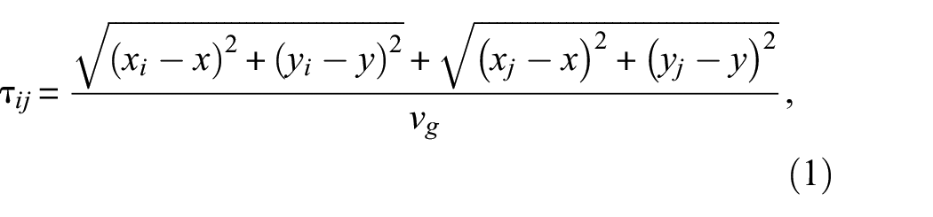
This section introduces the basic principle of the ellipse imaging algorithm24,25 and its characteristics (statistical characteristics and fuzzy characteristics). Figure 1 shows a schematic diagram of the principle and characteristics of the elliptical imaging algorithm. Figure 1(a) shows the principle of elliptical imaging. As illustrated in Figure 1(a), when the positions of the excitation sensor, the receiving sensor, and the defect are fixed, the sum of the distance
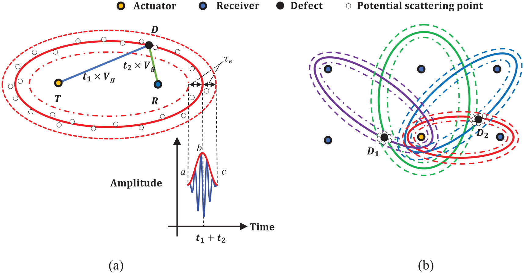
Schematic diagram of the principle and characteristics of the elliptical imaging algorithm: (a) the principle of elliptical imaging and (b) the statistical and fuzzy characteristics of the ellipse imaging algorithm.
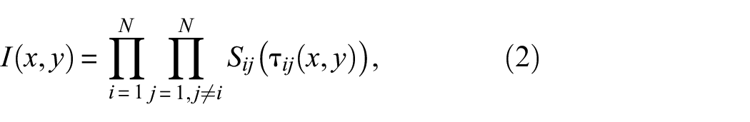
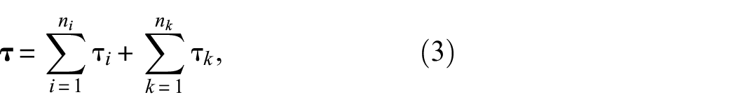
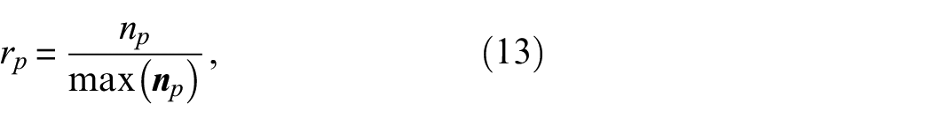
In the ellipse imaging algorithm, the accuracy of the defect location can be improved by fusing the amplitude information of the scattered signals of different inspection pairs. The fused mathematical function can be expressed as shown in Equation (2). In actual detection, due to the influence of the experimental conditions, the arrival time vector of the scattered signals usually consists of the arrival time vector of the defect scattered signals and the arrival time vector of the interference signals such as the edge scattered signals or noise scattered signals of the specimen. This can be expressed as shown in functional Equation (3).
where
where
Figure 1(b) shows the statistical and fuzzy characteristics of the ellipse imaging algorithm. The statistical characteristics mean that the number of elliptical arcs passing through the defects is higher than that for other positions. In the figure, two elliptical arcs (the green elliptical arc and purple elliptical arc) intersect at
The fuzzy characteristics mean that in elliptical imaging, even if there is a slight deviation between the measured data and the actual value, the detection result is still reliable. In Figure 1(b), only the blue elliptical arc and red elliptical arc pass through the position of defect
Evolutionary algorithm
As described in the “Elliptical imaging algorithm” section, there are potential scattering points in the zone where the elliptical arcs intersect, and these can be used to identify the locations of the defects. In this study, the problem of defect location is transformed into the problem of a scattering point search for analysis. The evolutionary algorithm 21 is selected to perform the search process. The execution steps of the evolutionary algorithm are as follows.
Step 1: The objective function is optimized. An optimized objective function is constructed based on the kernel function and the analysis objective.
Step 2: The population is initialized. The boundary of the variable
Step 3: Population screening is performed. Based on the optimized objective function, the residual value and fitness value of the population are calculated, analyzed, and screened to keep
Step 4: The cut-off criteria are determined. If the individual fitness meets the predefined cut-off threshold or reaches the maximum generation number, the analysis is finished. Otherwise, the generation number is updated to continue the analysis.
Step 5: The population update is performed, in which parents are added to the Gaussian or uniformly distributed random variables with average parent parameters for the individual update to obtain offspring populations, and eligible offspring individuals are combined with their parents to construct a new generation of analysis individuals. Then the algorithm returns to step 3.
K-means clustering algorithm
Combined with the characteristics of the elliptic imaging algorithm, the evolutionary algorithm is improved and the K-means algorithm
21
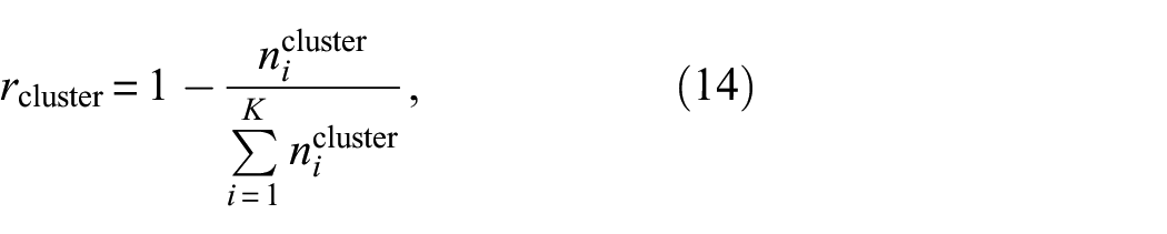
is applied to the steps of population screening and population updating, which preserves the statistical characteristics of individuals and ensures the reliability of the defect detection algorithm. In population screening, the K-means clustering algorithm is used for individual screening. When the sizes of the analyzed individuals are larger than
The clustering algorithm divides the data sets into different classes or clusters according to specific measurement rules and ensures that the similarity of individuals in the same cluster is as great as possible and the differences between individuals in different clusters are as great as possible. The execution process of the K-means algorithm is as follows.
(1) The
Improved intelligent defect location algorithm
In this study, the intelligent defect location algorithm is improved and the influence of a U-shaped boom structure on the propagation characteristics of helical guided waves is considered. We modify the matching and screening of the individual distance in the intelligent defect location algorithm to the matching and screening of the individual arrival time, which makes the algorithm more suitable for the defect detection of a U-shaped boom and simplifies the intelligent defect location algorithm by ensuring the defect location accuracy. Figure 2 shows the flowchart of the improved intelligent defect location algorithm. The detailed implementation process is as follows.
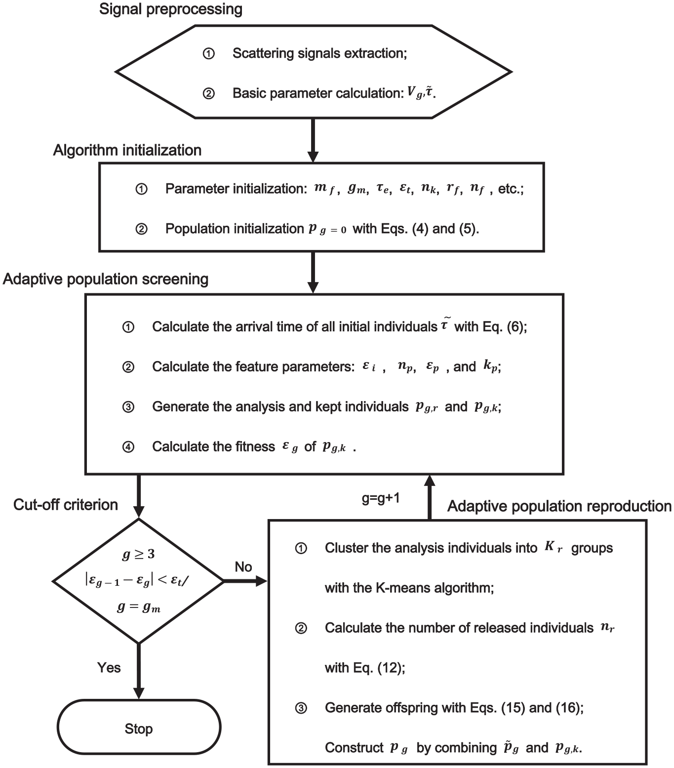
Flowchart of the improved intelligent defect location algorithm.
Step 1: Signal preprocessing. (1) The scattering signal, which is obtained using the difference between the damage signal and the reference signal, is extracted. (2) The basic parameters are calculated, the arrival time vector
Step 2: Algorithm initialization. (1) The basic parameters are initialized, and the parameter range vector


where L and U are the lower and upper boundary notations of
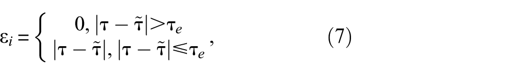
Step 3: Adaptive population screening. (1) The arrival time of all initial individuals

where
where

where


where
Step 4: Cutoff criteria. If the number of generations is greater than three and the population fitness of adjacent generations is less than the cut-off threshold, or the maximum generation number
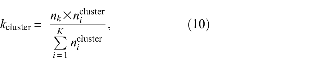
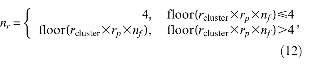
Step 5: Adaptive population reproduction. (1) The K-means clustering algorithm is used to divide the analysis individuals
where
where
Numerical and experimental setups
As concluded in References 7–13, in a relatively thin-walled pipe, ultrasonic guided waves regard a pipe as a curved plate-like structure, and ultrasonic guided waves can be approximated as Lamb waves propagating along a helical path. A U-shaped boom is a thin-walled tube with a U-shaped cross-section. The whole structure is welded with upper and lower steel plates with different thicknesses. The upper steel plate is rolled and bent into a 5 mm thick U-shaped steel plate, and the lower steel plate is bent into a 4 mm thick U-shaped steel plate through a die. Therefore, the structure of a U-shaped boom is complicated. The cross-sectional dimensions of a U-shaped boom are presented in Figure 3. It can be seen from Figure 3 that a U-shaped boom has a symmetrical structure. The black box in the figure is marked as a partially enlarged view of the welded structure. The dispersion curve of the guided waves in the plate is drawn according to the cross-section size and material parameters of a U-shaped boom. The material parameters are shown in Table 1. The DISPERSION software program is used to draw the dispersion curves of steel plates with different thicknesses. Figure 4 depicts the dispersion curves of Lamb waves in the 4 and 5 mm thick steel plates for the (a) phase velocity and (b) group velocity. As shown in Figure 4, the solid blue line represents the dispersion curve of the steel plate with a thickness of 5 mm. The solid red line indicates the dispersion curve of a 4 mm steel plate. To reduce the mutual interference of multi-modes, the frequency region with only two fundamental modes (A0 and S0) is selected as the selection region. Through observation, it is determined that the A0 mode used in our study has an excitation frequency of 150 kHz. The reasons for this are as follows: (a) at this frequency, the A0 mode has a relatively flat group velocity dispersion curve and a relatively dispersed phase velocity dispersion curve. (b) At this frequency, the wavelength of the A0 mode is less than that of the S0 mode, which meets the requirements for the ability to identify hole defects.
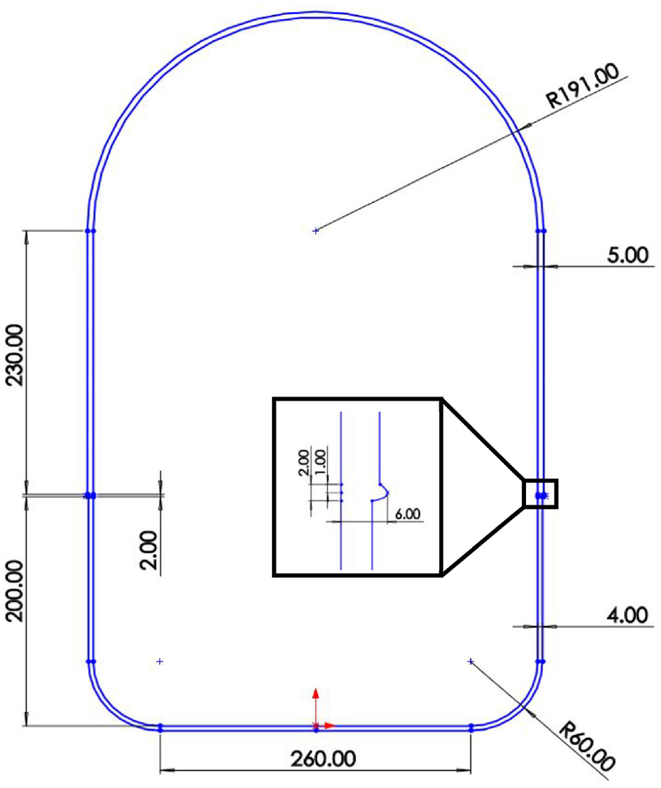
Cross-sectional dimensions of a U-shaped boom.
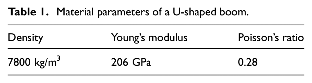
Material parameters of a U-shaped boom.
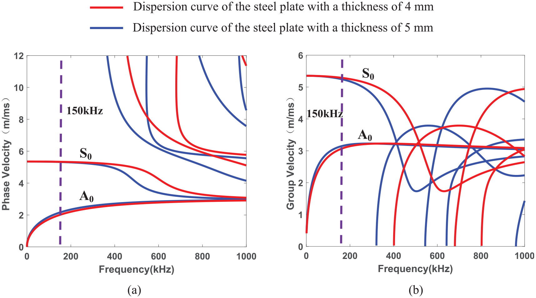
Dispersion curves of Lamb waves in 4 and 5 mm thick steel plates. (a) Phase velocity and (b) group velocity.
The following section describes how the propagation characteristics of helical guided waves in a U-shaped boom are studied with numerical and experimental research. For simplicity, we assume that the ultrasonic guided waves propagate along a straight path in the U-shaped boom. 7
Finite element model
The finite element models of three U-shaped booms are established with the software program ABAQUS, as shown in Figures 5 and 6. The cross-sectional dimensions and the lengths of the three models are exactly the same. The cross-sectional dimensions are shown in Figure 3, and the length is 1510 mm. The mesh type at the weld and near the defect of the model is C3D6, and the mesh type for the other parts is C3D8R (
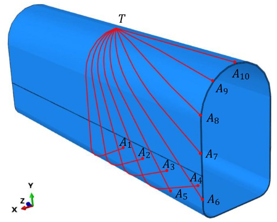
Finite element model that is used to analyze the propagation characteristics of helical guided waves in a U-shaped boom.
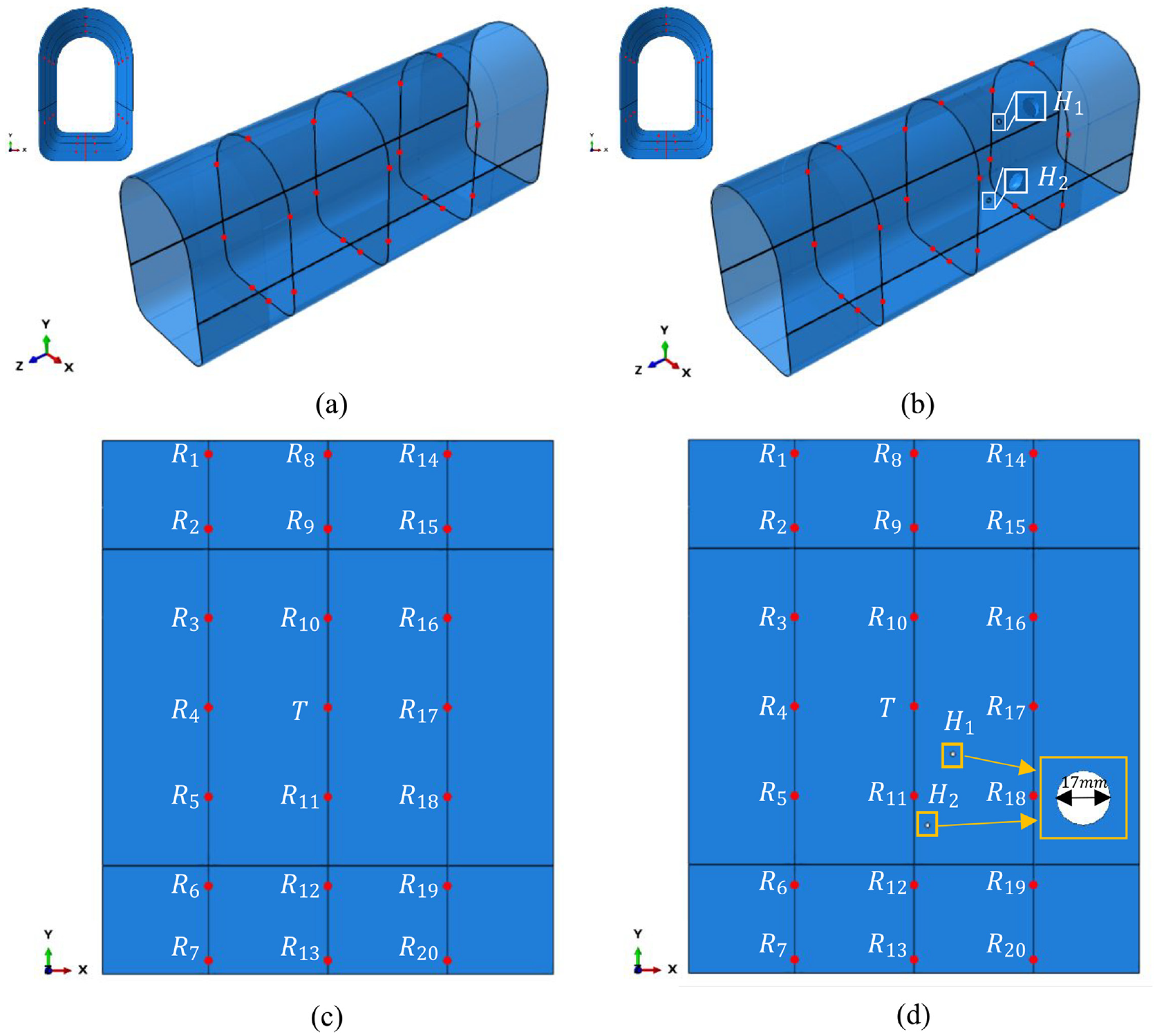
Finite element model that is used to verify the effectiveness of the improved intelligent localization algorithm. (a) The model of the normal structure, (b) the model of the damaged structure, (c) the unwrapped plate corresponding to (a), and (d) the unwrapped plate corresponding to (b).
Figure 5 shows the finite element model that is used to analyze the propagation characteristics of the helical guided waves in a U-shaped boom. To study the propagation characteristics of helical guided waves with different propagation paths, 10 different ray paths (T-A1–T-A10) are set as the receiving paths for signal acquisition (point-by-point acquisition). As shown by the solid red line in Figure 5, the angular interval between each path is 10 degrees. At this point, T is the excitation point, and a concentrated force is applied to excite Lamb waves.
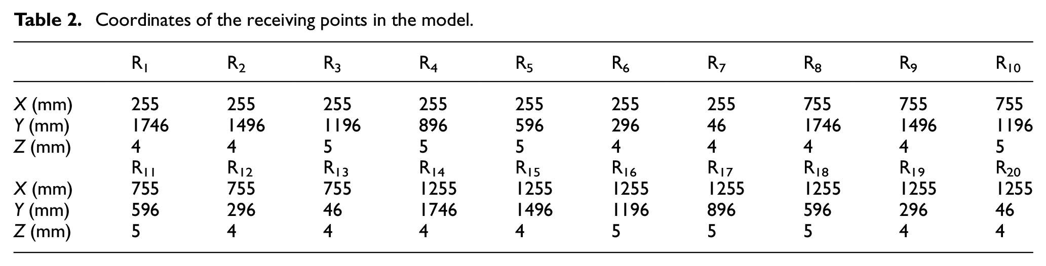
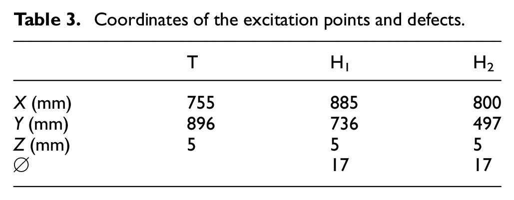
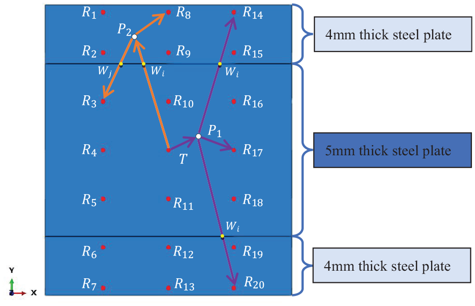
Figure 6 shows the finite element model that is used to verify the effectiveness of the improved intelligent localization algorithm. Figure 6(a) shows the model of the normal structure and Figure 6(b) shows the model of the damaged structure. The red dots in the figure are excitation points and receiving points, which are arranged in three circular arrays, and the upper left corner of the figure is the left view of the U-shaped boom. The solid red line is the axis symmetry line of the U-shaped boom, and the U-shaped boom is unfolded along the axis symmetry line to obtain the corresponding unwrapped plate, as shown in Figure 6(c) and (d). Figure 6(c) shows the unwrapped plate corresponding to Figure 6(a) and (d) shows the unwrapped plate corresponding to Figure 6(b). In Figure 6(b), two circular through-hole defects with a diameter of 17 mm are introduced in the model. T is the excitation position, which is consistent with the position of point T in Figure 5, and R1–R20 are the receiving positions. The receiving positions in Figure 6(a) and (b) acquire the reference signal and the detection signal, respectively. In the numerical simulation, the out-of-plane displacement is extracted as the helical guided wave analysis signal. The coordinates of the receiving points in the unwrapped plate are listed in Table 2, and the coordinates of the excitation points and defects are listed in Table 3.
Coordinates of the receiving points in the model.
Coordinates of the excitation points and defects.
Experimental setup
We conduct two experimental studies. The first study involves the examination of the propagation characteristics of helical guided waves in the U-shaped boom, and the other study involves the detection of the double-hole defects to verify the effectiveness of the improved intelligent algorithm. The experimental setup (see Figure 7) consists of the function generator, power amplifier, oscilloscope, piezoelectric sensors (PZTs), and U-shaped boom sample. The diameter and the thickness of the piezoelectric sensor are 10 and 0.5 mm, respectively. Figure 7(a) displays the experimental setup for the detection of the propagation characteristics of the helical guided waves. To facilitate comparative analysis, the location of the excitation point in the experiment is the same as that in the finite element model. The excitation is a five-cycle tone burst centered at 150 kHz, consistent with the excitation signal in Section “Finite element model”. The receiving paths in the experiment correspond to the simulated receiving paths. However, unlike the simulation study, in the experiment, the sensors in each receiving path are arranged at 50 mm intervals, and attached to the U-shaped boom by a shear wave coupling agent. The numbers of receiving points for the T-A1–T-A10 receiving paths are 18, 18, 19, 20, 15, 14, 11, 10, 10, and 10. Figure 7(b) shows the experimental setup for the detection of double-hole defects. The location of the excitation point T, the location of the receiving points (R1–R20), and the selection of the excitation signals are consistent with those in the finite element model. In the above experiment, the T-point piezoelectric sensor is used as the exciter, and the other sensors are used as the receivers to capture the Lamb wave signals.
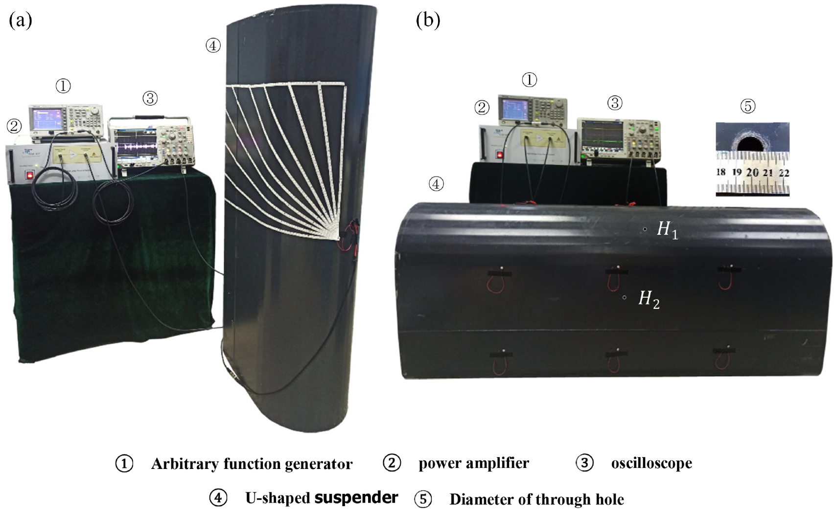
Experimental setup (a) for the detection of the propagation characteristics of the helical guided waves and (b) for the detection of double-hole defects.
Analysis of the propagation characteristics of helical guided waves
In the formation process of the helical guided waves in the U-shaped boom, Lamb waves are generated by the loading concentrated force at the excitation point T. Lamb waves form a circular wavefront with the excitation point T as the center, and the circular wavefront spreads in the U-shaped boom at countless angles, thus forming the guided waves that propagates along the helical path, that is, a helical guided waves. Because of the welding seam and the variable thickness in a U-shaped boom, this research is focused on the influence of the welding seam and the different wall thicknesses on the propagation characteristics of the helical guided waves. Figure 8 shows the simulated time-space wave fields of different receiving paths. The receiving paths of T-A1, T-A2, T-A3, T-A4, T-A5, and T-A6 pass through the weld area. From the space-time wave field in Figure 8(a) to (f), it can be found that with the increase of the propagation distance of the helical guided waves, the wave field is gradually separated from one wave packet into two wave packets, corresponding to the A0 mode Lamb waves and the S0 mode Lamb waves. When the wave packet propagates to the weld, the A0 mode Lamb waves and the S0 mode Lamb waves produce an obviously reflected wave packet and a mode converted wave packet in which the A0 mode wave energy is higher and the reflected wave, transmitted wave, and mode converted wave are more obvious. Therefore, in this research, the A0 mode is chosen as the main research object. In the receiving paths of T-A5 and T-A6, because of the acquisition distance, there is no mode conversion wave packet in the space-time wave field. The above phenomena of wave reflection, mode conversion, and transmission describe the wave propagation characteristics of the interaction between the helical guided waves and weld structures.

Simulated time-space wave fields of different receiving paths: (a) T-A1 receiving path, (b) T-A2 receiving path, (c) T-A3 receiving path, (d) T-A4 receiving path, (e) T-A5 receiving path, (f) T-A6 receiving path, (g) T-A7 receiving path, (h) T-A8 receiving path, (i) T-A9 receiving path, and (j) T-A10 receiving path.
As shown in Figure 8(g) to (j), the helical guided wave propagates directly from the excitation point T to the end of the U-shaped boom. From the space-time wave field, it can be seen that with the increase of the propagation distance, the A0 mode wave packet propagates in a straight line, and obvious boundary reflection waves are generated at the end of the U-shaped boom. The wave reflection phenomenon discussed above describes the wave propagation characteristics of the interaction between the helical guided waves and the boundary of the U-shaped boom.
Figure 9 shows the experimental time-space wave fields of different receiving paths. It also shows the same helical guided wave propagation characteristics, as described in the simulated time-space wave field. However, the mode conversion wave packet at the weld is weak, as shown in Figure 9, and the wave packet is submerged in noise and cannot be identified.
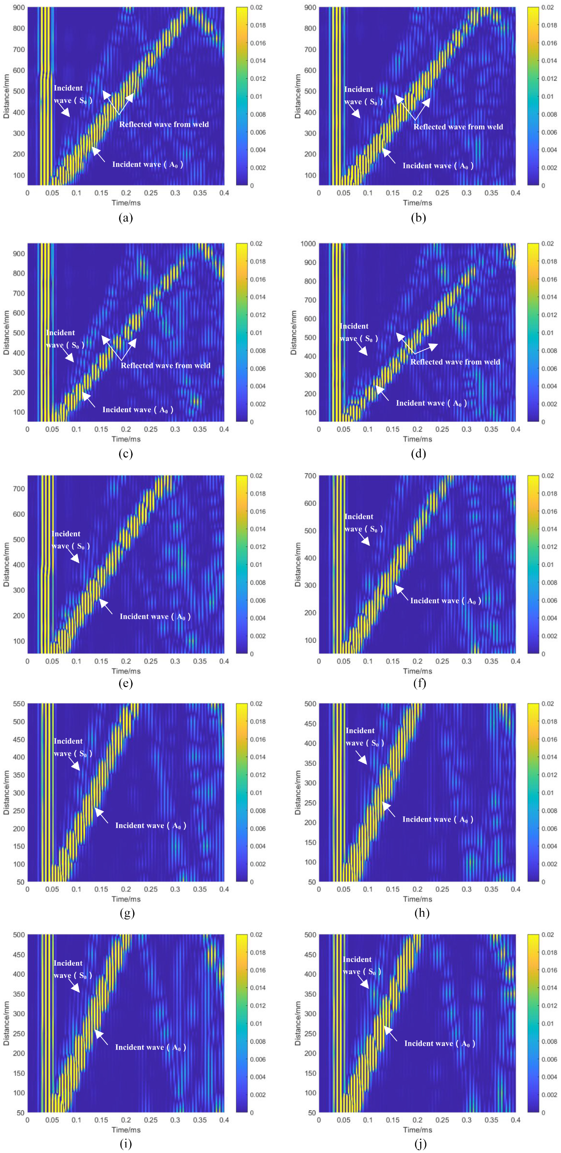
Experimental time-space wave fields of different receiving paths (a) T-A1 receiving path, (b) T-A2 receiving path, (c) T-A3 receiving path, (d) T-A4 receiving path, (e) T-A5 receiving path, (f) T-A6 receiving path, (g) T-A7 receiving path, (h) T-A8 receiving path, (i) T-A9 receiving path, and (j) T-A10 receiving path.
By extracting the arrival time of the A0 mode of the incident wave in the simulated wave field and the experimental wave field, the change of the group velocity of the A0 mode helical guided waves with different wall thicknesses is analyzed. Figure 10 displays the fitting curve of the A0 mode arrival time of the T-A1 receiving path in the numerical and experimental studies. Figure 10(a) presents the numerical result. The fitting formula indicates that the arrival time of the A0-mode fits well for different wall thicknesses, and the group velocities of the helical guided waves are 3.087 m/ms in the tube with a 5 mm wall thickness and 3.033 m/ms in the tube with the 4 mm wall thickness. Figure 10(b) shows the experimental result. In the experiment, the arrival time of the A0 mode is also well fitted. The group velocities of the helical guided waves are 3.153 m/ms in the tube with a 5 mm wall thickness, and 2.932 m/ms in the tube with a 4 mm wall thickness. Based on the above method, the arrival times of the A0 modes in other receiving paths are analyzed in turn, and the A0 mode group velocities of the helical guided waves with different paths and different wall thicknesses are obtained.
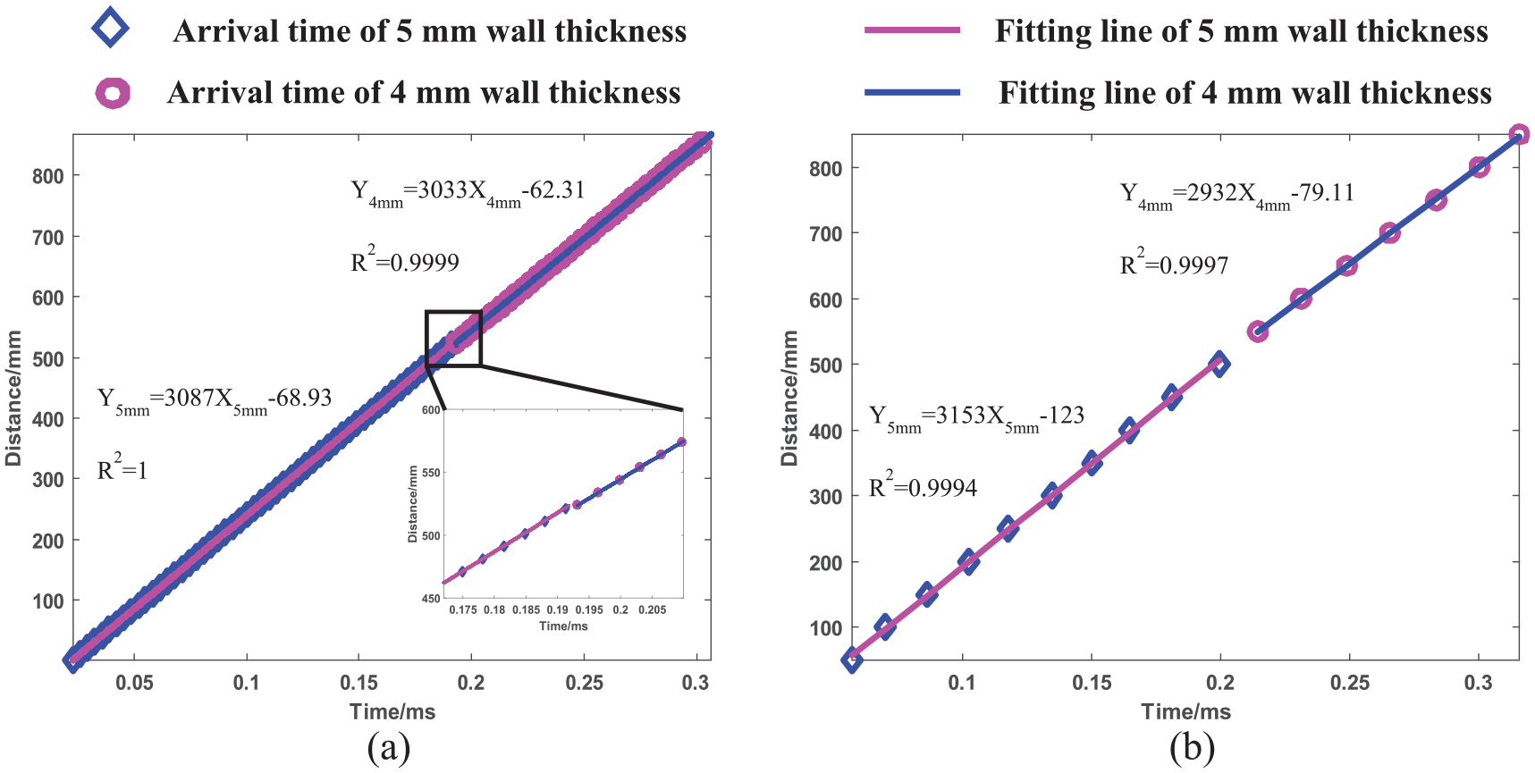
Fitting curve of the A0 mode arrival time of the T-A1 receiving path in the numerical and experimental studies: (a) the numerical result and (b) the experimental result.
A statistical analysis of the group velocities with different wall thicknesses is conducted. According to the dispersion curves of the Lamb waves in the 4-mm- and 5-mm-thick steel plates shown in Figure 4, the theoretical group velocities of the A0 mode are 3.120 m/ms for a 5 mm wall thickness and 3.033 m/ms for a 4 mm wall thickness. Figure 11 shows the boxplot of the A0 mode group velocity with the wall thicknesses of 5 mm and 4 mm. Figure 11(a) shows the group velocity obtained by the numerical signals with the wall thickness of 5 mm, and Figure 11(b) shows the group velocity obtained by the experimental signals with the wall thickness of 5 mm. It can be seen from the figure that the average group velocity of the simulation signal is 3.095 m/ms, and the average group velocity of the experimental signal is 3.147 m/ms, which is very close to the theoretical group velocity of 3.120 m/ms. Figure 11(c) shows the group velocity obtained by the numerical signals with the wall thickness of 4 mm, and Figure 11(d) shows the group velocity obtained by the experimental signals with the wall thickness of 4 mm. At the wall thickness of 4 mm, the average group velocity of the simulation signal is 2.983 m/ms, and that of the experimental signal is 3.001 m/ms, both of which are close to the theoretical group velocity (3.033 m/ms), so the simulation results are in good agreement with the experimental results. There are many differences in the group velocity values for different wall thicknesses, whether for the simulation results or the experimental results. Therefore, when detecting the defects of a U-shaped boom, the influence of the different propagation speeds of the helical guided waves for different wall thicknesses on the defect location should be considered to improve the accuracy of the defect location.
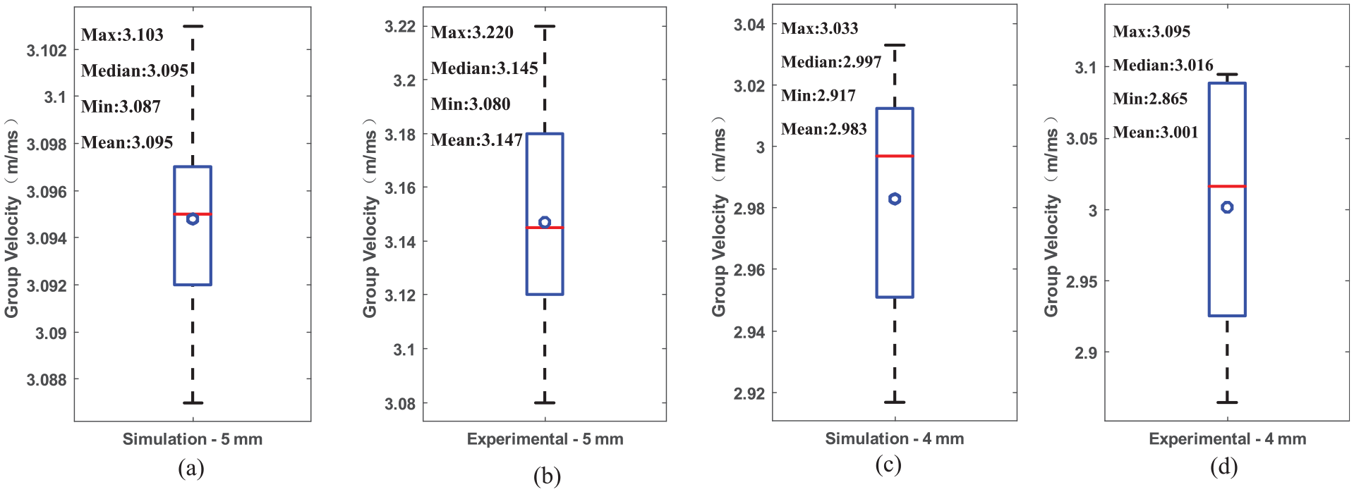
Boxplot of the A0 mode group velocity with wall thicknesses of 5 and 4 mm: (a) the group velocity obtained by the numerical signals with the wall thickness of 5 mm, (b) the group velocity obtained by the experimental signals with the wall thickness of 5 mm, (c) the group velocity obtained by the numerical signals with the wall thickness of 4 mm, and (d) the group velocity obtained by the experimental signals with the wall thickness of 4 mm.
Verification of improved intelligent defect location algorithm
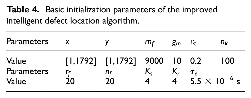
The basic initialization parameters of the improved intelligent defect location algorithm are shown in Table 4. The parameter ranges are
Basic initialization parameters of the improved intelligent defect location algorithm.
Numerical validation
Figure 12 is the signal preprocessing of the T–R4 inspection pair. Figure 12(a) shows the detection signal and reference signal of the T–R4 inspection pair. The solid blue line is the reference signal and the dotted pink line is the detection signal. The scattering signal is obtained using the difference between the detection signal and the reference signal. Figure 12(b) shows the T–R4 inspection pair of the received scattered signals. In the figure, the scattered signal and its envelope are drawn with blue and red solid lines, respectively, the extreme points of four different wave packets are marked with green circles, and the red dotted line is the extracted signal based on the extracted extreme points and the arrival time-dependent screening threshold
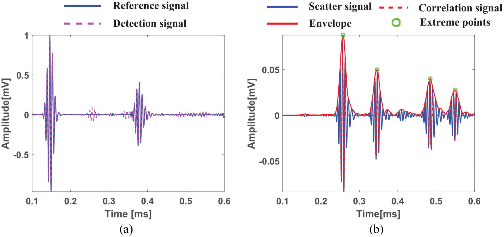
Signal preprocessing of the T–R4 inspection pair. (a) The detection signal and the reference signal of the T–R4 inspection pair and (b) the T–R4 inspection pair of the received scattered signals.
As discussed in the “Analysis of the propagation characteristics of helical guided waves” section, the average group velocity of the simulation signal is 3.095 m/ms when the wall thickness is 5 mm and 2.982 m/ms when the wall thickness is 4 mm. Figure 13 shows the imaging results of the T–R4 inspection pair for different group velocities. Figure 13(a) shows the elliptical imaging results of the T–R4 inspection pair with Vg = 3.095 m/ms. Figure 13(b) shows the elliptical imaging results of the T–R4 inspection pair with Vg = 2.982 m/ms. The black points in the figure represent the defect position, and the blue points represent the sensor position. Figure 13(a) and (b) shows four elliptical arcs with T and R4 as the focus. In Figure 13(a), two elliptical arcs pass through the defect position. The other two elliptical arcs do not pass through the defect position. According to Equation (3), it can be inferred that the elliptical arc that does not pass through the defect position is an interference wave. However, due to the difference in the group velocity between Figure 13(a) and (b), there is a slight deviation between the elliptical arc region and the defect position in Figure 13(b). The distribution results of the kept individuals are determined according to Equations (6) and (7). Figure 13(c) shows the distribution of the kept individuals of the T–R4 inspection pair with Vg = 3.095 m/ms. Figure 13(d) shows the distribution of the kept individuals of the T–R4 inspection pair with Vg = 2.982 m/ms. The gray and red dots represent the kept individuals and defects, respectively, and the kept individuals are distributed in the yellow influence zone, which is obtained based on the arrival time vector of the wave packets and the screening threshold
Imaging results of the T–R4 inspection pair for different group velocities. (a) The elliptical imaging results of the T–R4 inspection pair with Vg = 3.095 m/ms, (b) the elliptical imaging results of the T–R4 inspection pair with Vg = 2.982 m/ms, (c) the distribution of the kept individuals of the T–R4 inspection pair with Vg = 3.095 m/ms, and (d) the distribution of the kept individuals of the T–R4 inspection pair with Vg = 2.982 m/ms.
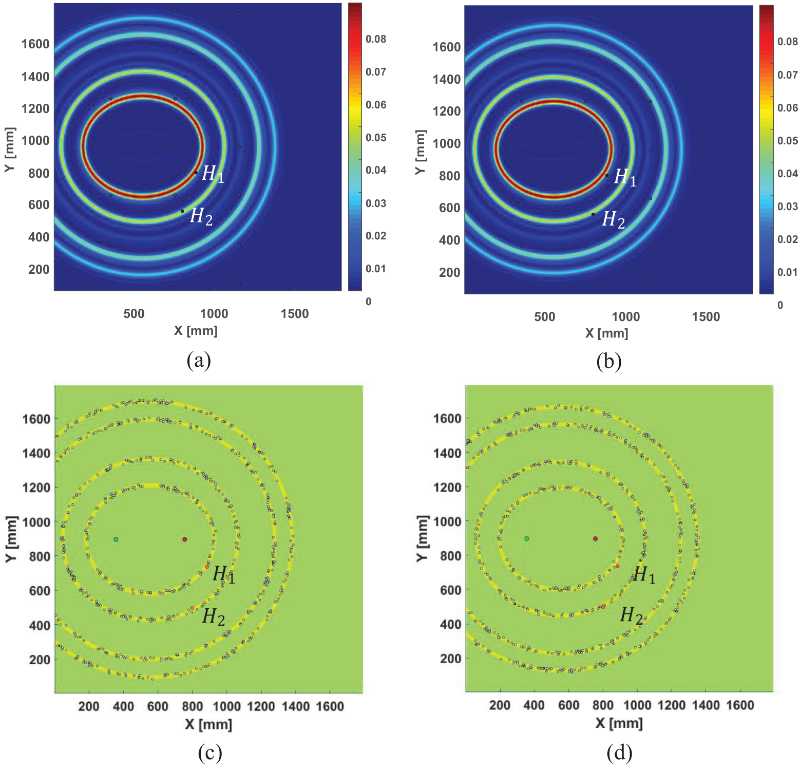
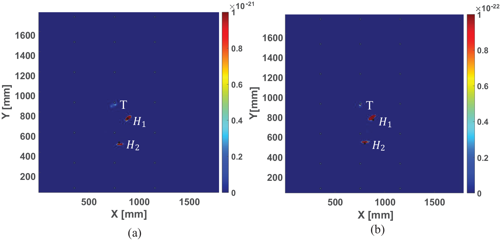
The elliptical imaging results of all inspection pairs fused at different group velocities are drawn using mathematical functional Equation (2). Figure 14 shows the elliptical imaging results of all inspection pairs fused at different group velocities. Figure 14(a) shows the elliptical imaging results with Vg = 3.095 m/ms. When only considering the group velocity Vg = 3.095 m/ms with a wall thickness of 5 mm, the regions with higher pixel values in Figure 14(a) are distributed near defects H1 and H2. Although there is a small deviation between the location of defect H2 and the highlighted area, the initial location of the defect can still be determined. Figure 14(b) shows the elliptical imaging results with Vg = 2.982 m/ms. When only considering the group velocity Vg = 2.982 m/ms with a wall thickness of 4 mm, there is a deviation between the high pixel value area and the positions of defects H1 and H2, both of which are above the positions of the defects, which proves that when only the group velocity with a wall thickness of 4 mm is considered, the positioning of the defects has deviated, and the accurate positioning of the defects cannot be achieved.
Elliptical imaging results of all inspection pairs fused at different group velocities. (a) The elliptical imaging results with Vg = 3.095 m/ms and (b) the elliptical imaging results with Vg = 2.982 m/ms.
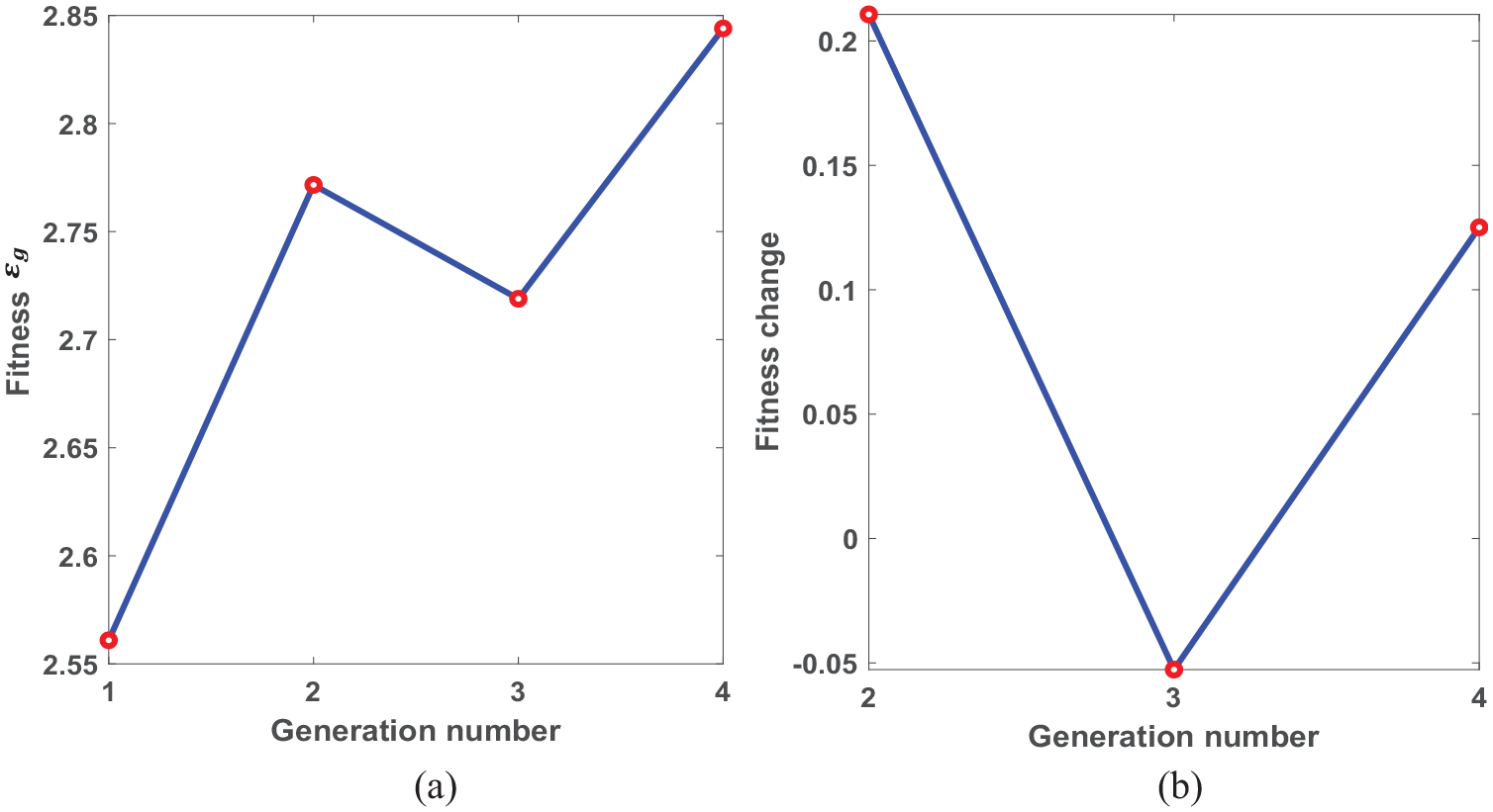
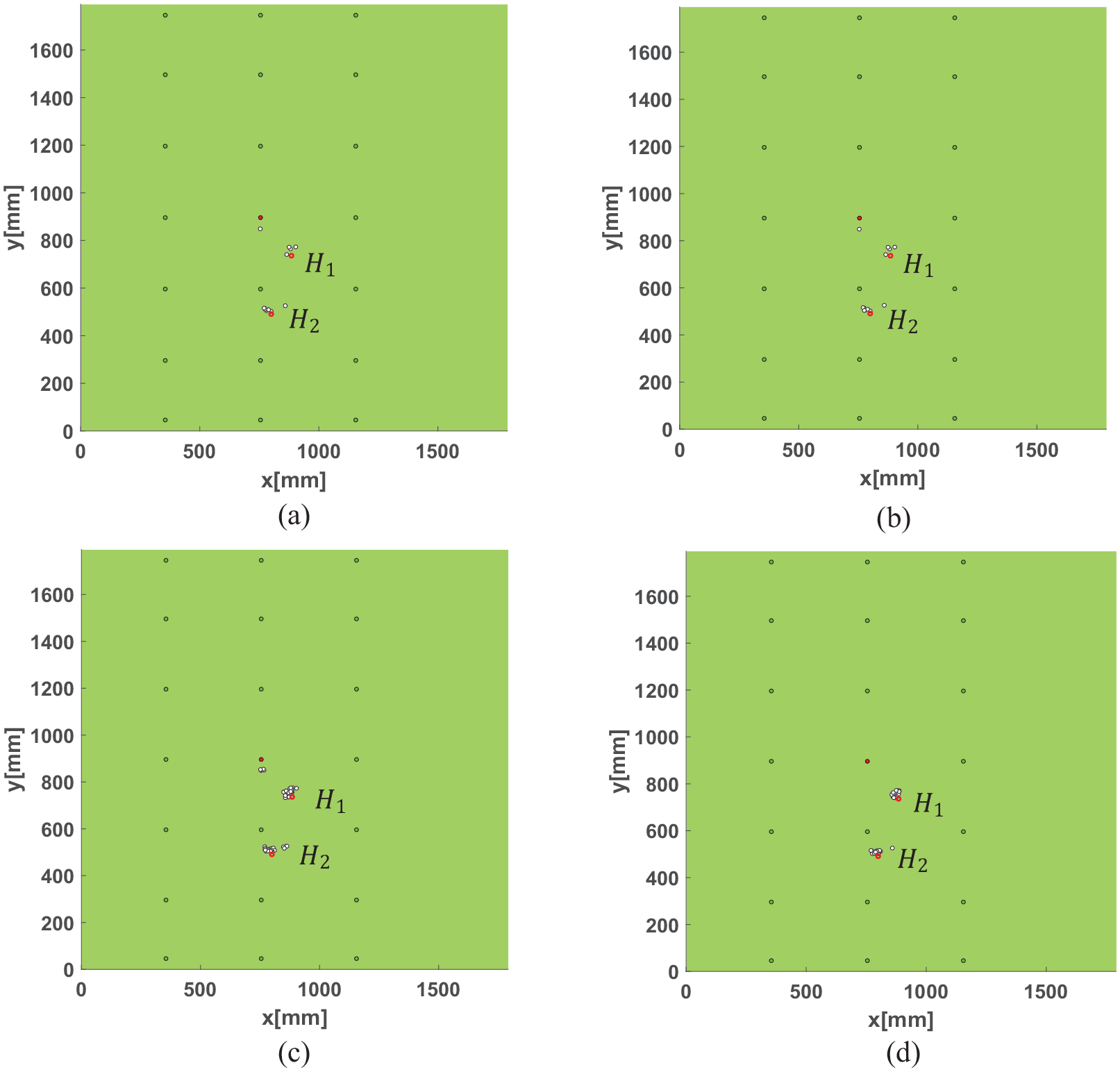
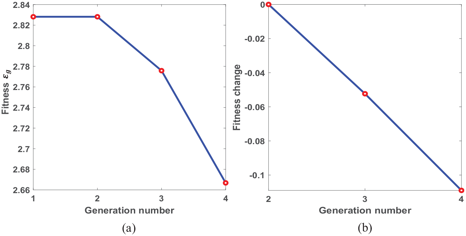
The improved intelligent defect location algorithm is used to analyze the simulation signal. The convergence curve of the improved intelligent defect location algorithm with Vg = 3.095 m/ms is shown in Figure 15. Figure 15(a) displays the convergence curve of the population fitness, in which the fitness value changes randomly. Figure 15(b) displays the gradient curve of the population fitness. The gradient change between the third generation and the fourth generation is less than the predetermined cut-off threshold of 0.2. Therefore, the algorithm stops in the fourth generation. Figure 16 shows the improved intelligent defect location result with Vg = 3.095 m/ms. Figure 16(a) to (d) show the kept individuals from the first generation to the fourth generation. With the increase of the iterative algebra, the kept individuals gradually converge around defects H1 and H2. The distribution area of the kept individuals in Figure 16(d) is in good agreement with the elliptical imaging results in Figure 14(a), which can achieve the preliminary localization of the defects. Figure 17 shows the convergence curve of the improved intelligent defect location algorithm with Vg = 2.982 m/ms. It can be seen from the figure that the gradient change of the fourth generation meets the cut-off criterion, and the algorithm stops in the fourth generation. Figure 18 shows the improved intelligent defect location result with Vg = 2.982 m/ms. The kept individuals gradually gather near the defects from the third generation and converge near the defects in the fourth generation. The distribution area of the kept individuals in Figure 18(d) is in good agreement with the highlighted area in Figure 14(b). Through the above analysis, it can be found that when the group velocity is the same, the imaging results of the improved intelligent defect location algorithm are in good agreement with those of the elliptical imaging algorithm, which verifies the effectiveness of the improved intelligent defect location algorithm.
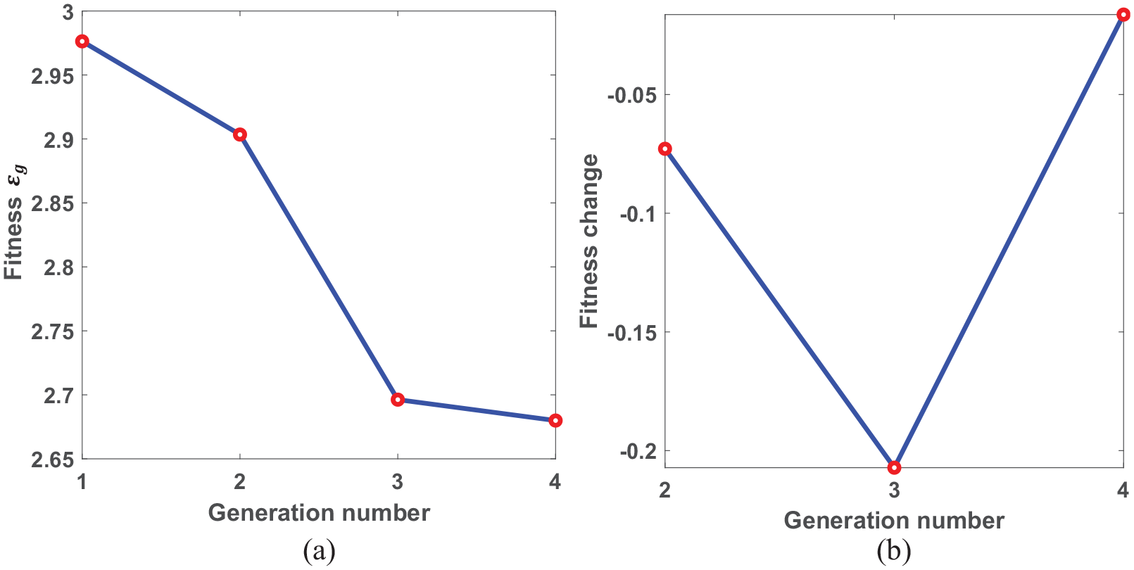
Convergence curve of the improved intelligent defect location algorithm with Vg = 3.095 m/ms. (a) The convergence curve of the population fitness and (b) the gradient curve of the population fitness.
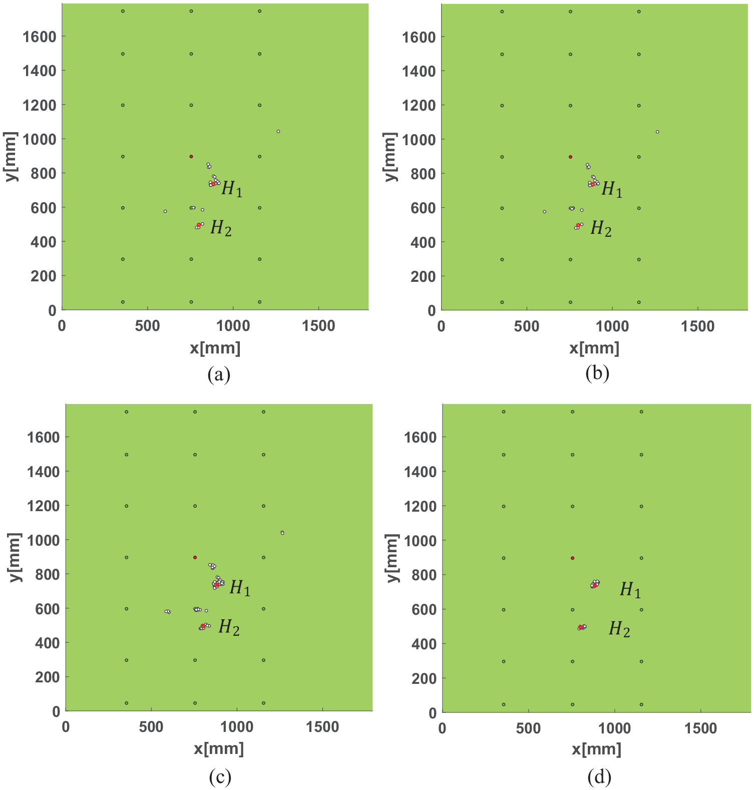
Improved intelligent defect location result with Vg = 3.095 m/ms. (a) g = 1, (b) g = 2, (c) g = 3 and (d) g = 4.
Convergence curve of the improved intelligent defect location algorithm with Vg = 2.982 m/ms. (a) The convergence curve of the population fitness and (b) the gradient curve of the population fitness.
Improved intelligent defect location result with Vg = 2.982 m/ms. (a) g = 1, (b) g = 2, (c) g = 3 and (d) g = 4.
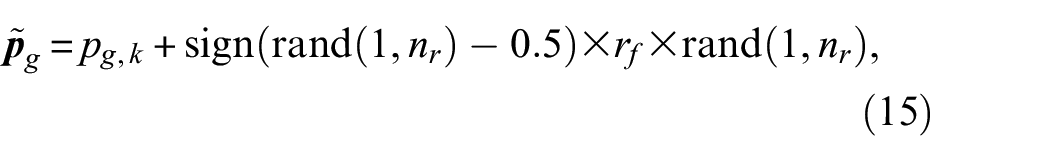
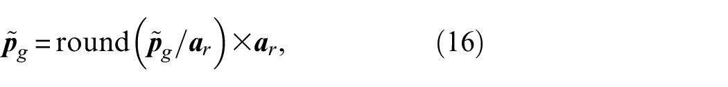
According to the above analysis, when only the group velocity with a wall thickness of 5 or 4 mm is considered, neither the elliptical imaging algorithm nor the improved intelligent defect location algorithm can achieve accurate defect location, so it is necessary to consider the factors of the group velocity of the helical guided waves that change with the wall thickness to improve the accuracy of the defect location. We propose an optimized adaptive screening scheme that fully considers the change of the group velocity of helical guided waves and uses the corresponding group velocity to accurately calculate the arrival time of each initial individual. We modify functional Equation (6) to improve the accuracy of the defect location. Figure 19 shows a schematic diagram for calculating the initial individual arrival time. The yellow dot represents the intersection of the helical guided wave propagation path and weld, and the white dot represents the initialization individual. The individuals


where
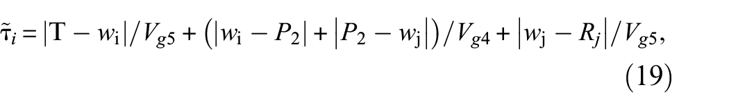

where
According to the above-mentioned optimization algorithm for the individual arrival time, the accuracy of the individual arrival time can be improved, and then the positioning accuracy of the optimized intelligent defect positioning algorithm can be improved by filtering through Equation (7).
Schematic diagram for calculating the initial individual arrival time
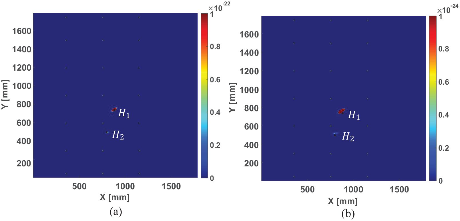
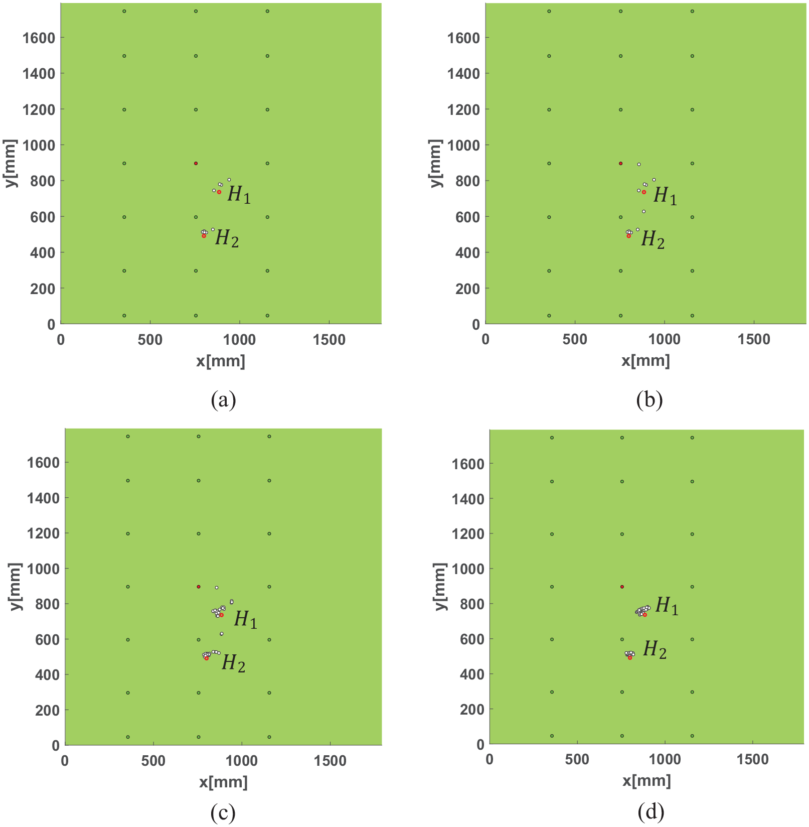
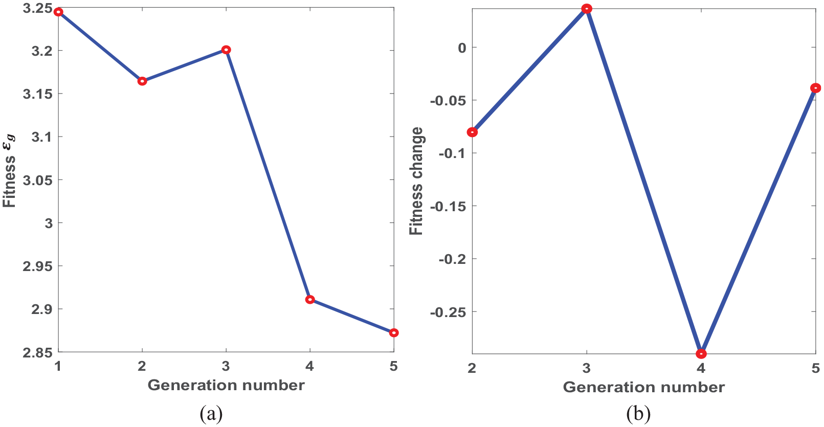
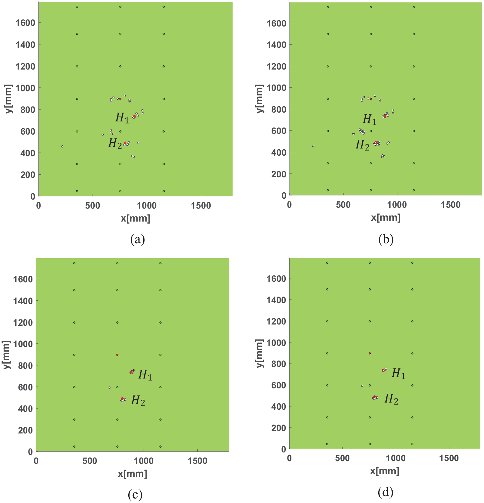
The optimized intelligent defect location algorithm is used to analyze the simulation signal. The convergence curve of the intelligent location algorithm is shown in Figure 20. Figure 20(a) displays the convergence curve of the population fitness, and the fitness value changes randomly. Figure 20(b) displays the gradient curve of the population fitness. The gradient change between the fourth generation and the fifth generation is less than the predetermined cut-off threshold of 0.2. Therefore, the algorithm stops in the fifth generation. Figure 21 shows the simulation signal imaging results of the optimized intelligent defect location algorithm, and Figure 21(a) to (d) shows the kept individuals in the second generation to the fifth generation. With the continuous clustering and screening, the kept individuals in Figure 21(d) gather around the defects. The distribution area of the kept individuals is very close to the location of the defects. Compared with Figure 16(d) and 18(d), the optimized intelligent location algorithm is more accurate in terms of the defect location.
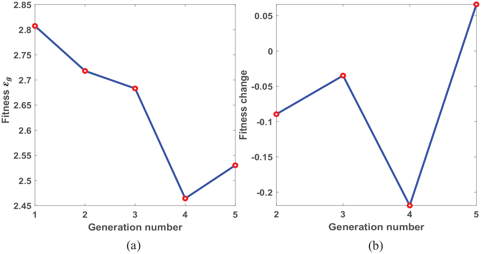
Convergence curve of the intelligent location algorithm. (a) The convergence curve of the population fitness and (b) the gradient curve of the population fitness.
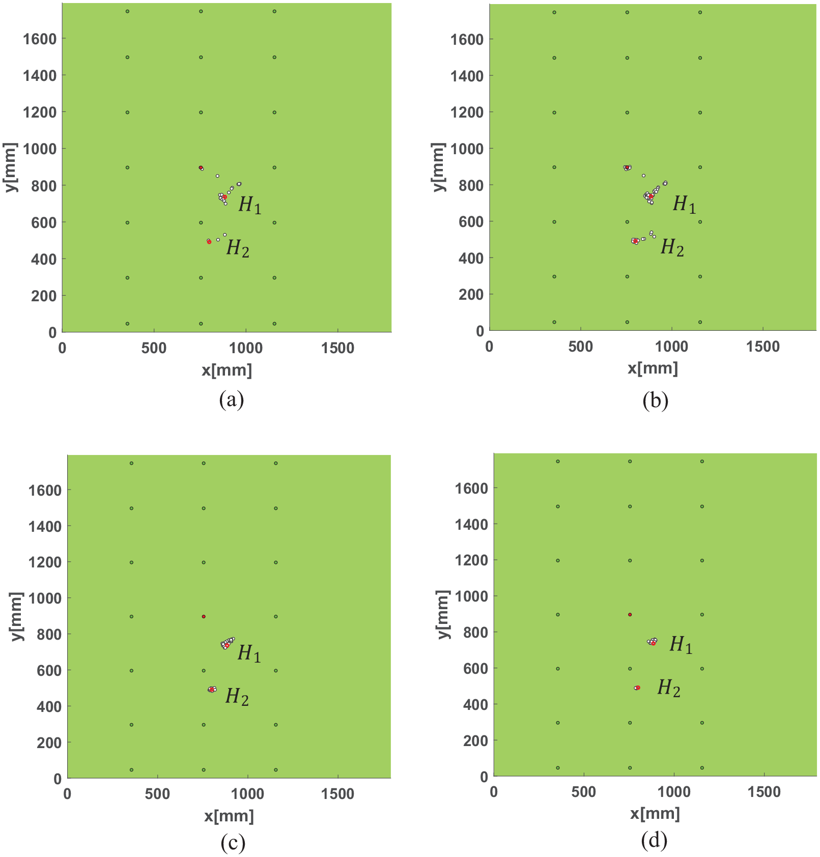
Simulation signal imaging results of the optimized intelligent defect location algorithm. (a) g = 2, (b) g = 3, (c) g = 4 and (d) g = 5.
Experimental validation
In the experiment, the piezoelectric sensor T is used as an actuator, and the rest of the piezoelectric sensors R1–R20 are used as receivers to capture helical guided wave signals. The sensor distribution is shown in Figure 6. First, in the experiment, a normal U-shaped boom is used to collect reference signals. Then the hole defects H1 and H2 are machined at different positions of the U-shaped boom. The two round holes have the same diameter of 17 mm. In the experiment testing the defect location, each receiving sensor performs collection three times, and a total of 20 × 3 = 60 sets of signals is obtained. According to the “Analysis of the propagation characteristics of helical guided waves” section, the average group velocity of the experimental signals is 3.147 m/ms when the wall thickness is 5 mm and 3.001 m/ms when the wall thickness is 4 mm.
Figure 22 shows the analysis of the double-hole detection signals received by the T–R4 inspection pair. Figure 22(a) shows the comparison of the reference signal and the detection signal. Figure 22(b) shows the preprocessing of the scattered signal of T–R4. The extraction of the extreme points involves extracting extreme points according to the interval between adjacent points and their amplitudes. If the interval between adjacent points is greater than 4 ms and their amplitudes are greater than 60% of the maximum values of all extreme points, the extreme points are extracted. There are many peaks in the envelope of the scattered signal, and this causes the extracted extreme points to deviate from the envelope peaks. Therefore, it is necessary to optimize the scattered signal and convolute the scattered signal with excitation to smooth its envelope optimization. Figure 22(c) shows the extreme points extracted from the optimized scattering signal. After optimization, the envelope peak of the scattered signal can be accurately extracted. The extreme points of four different wave packets are extracted, as shown in Figure 22(c), which is in good agreement with the positions of the extreme points of the simulation signal in Figure 12(b). Figure 22(d) shows the time–frequency diagram of the scattering signal. The time–frequency spectrum is obtained with a continuous wavelet transform in which the mother wavelet and the scale are set to “gaus4” and “5000”, respectively. The time–frequency analysis of the scattered signal in Figure 22(d) shows that the instantaneous frequencies of the four wave packets are all distributed at 150 kHz, which is consistent with the excitation frequency.
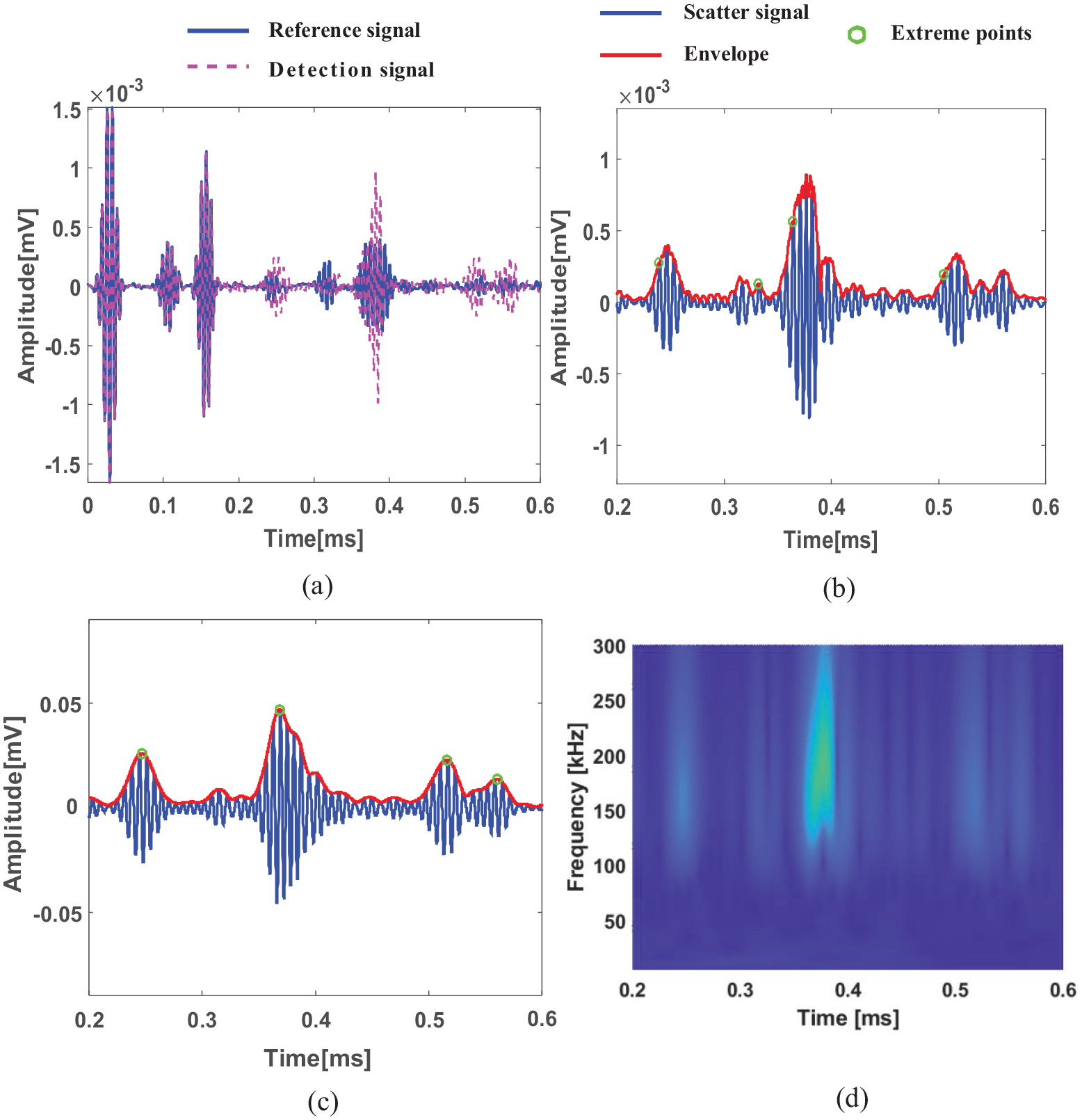
Analysis of double-hole detection signals received by the T–R4 inspection pair. (a) The comparison of the reference signal and the detection signal, (b) the preprocessing of the scattered signal of T–R4, (c) the extreme points extracted from the optimized scattering signal and (d) the time–frequency diagram of the scattered signal.
Figure 23 shows the elliptical imaging results of all inspection pairs fused at different group velocities. Figure 23(a) shows the elliptical imaging results with Vg = 3.147 m/ms. In Figure 23(a), the pixel value near defect H1 is high, which can be used to determine the accurate location of H1, but there is a deviation between H2 and the highlighted area. In addition, there is a false image at the excitation point T, but the low pixel value of the false image does not affect the defect location results. Figure 23(b) shows the elliptical imaging results with Vg = 3.001 m/ms. When only the group velocity Vg = 3.001 m/ms with a wall thickness of 4 mm is considered, there is a deviation between the highlighted area and the positions of the defects H1 and H2, which proves that the positioning of the defects deviates when only the group velocity with a wall thickness of 4 mm is considered, and the accurate positioning of the defects cannot be achieved.
Elliptical imaging results of all inspection pairs fused at different group velocities. (a) The elliptical imaging results with Vg = 3.147 m/ms and (b) the elliptical imaging results with Vg = 3.001 m/ms.
The experimental signal is analyzed with the improved intelligent defect location algorithm. The screening threshold of the arrival time of the scattered wave packets
Convergence curve of the improved intelligent defect location algorithm with Vg = 3.147 m/ms. (a) The convergence curve of the population fitness and (b) the gradient curve of the population fitness.
Improved intelligent defect location result with Vg = 3.147 m/ms. (a) g = 2, (b) g = 3, (c) g = 4, and (d) g = 5.
Convergence curve of the improved intelligent defect location algorithm with Vg = 3.001 m/ms. (a) The convergence curve of the population fitness and (b) the gradient curve of the population fitness.
Improved intelligent defect location result with Vg = 3.001 m/ms. (a) g = 1, (b) g = 2, (c) g = 3, and (d) g = 4.
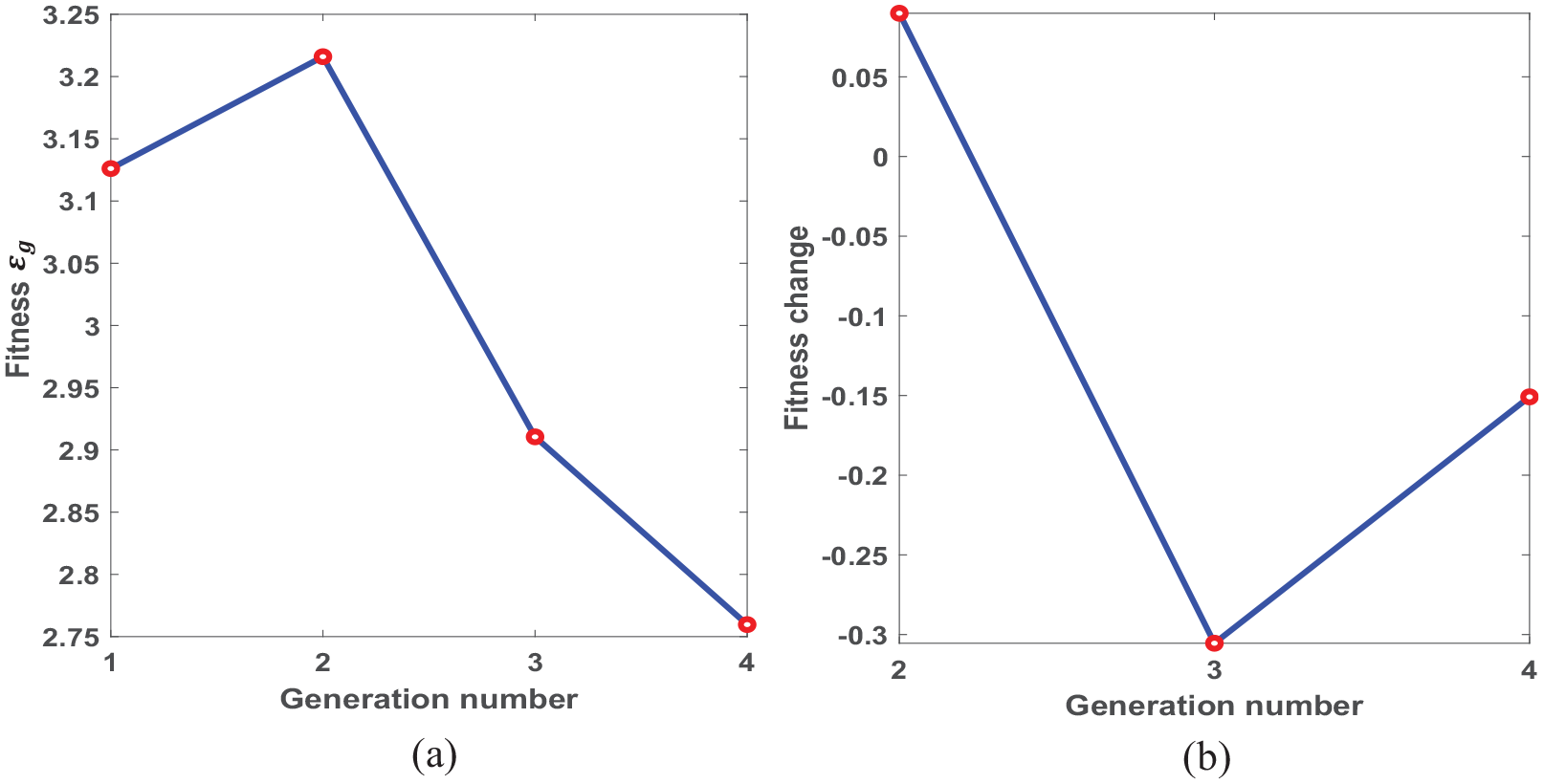
The optimized intelligent defect location algorithm is used to analyze the experimental signal. The convergence curve of the intelligent location algorithm is shown in Figure 28. The gradient change between the third generation and the fourth generation is less than the predetermined cut-off threshold of 0.2. The algorithm stops in the fourth generation. Figure 29 shows the imaging results of the experimental signal optimized intelligent defect location algorithm and Figure 29(a) to (d) show the reserved individuals of the first generation to the fourth generation. In Figure 29(a), the individuals are scattered and not clustered near H1 and H2. With the continuous population screening and population reproduction (Figure 29(d)), the retained individuals converge at the center of defects H1 and H2. Compared with Figure 25(d) and 27(d), the individuals in Figure 29(d) are completely concentrated around the defects H1 and H2, and there is no deviation from the individuals, which again proves that the optimized intelligent positioning algorithm effectively improves the defect positioning accuracy.
Convergence curve of the intelligent location algorithm. (a) The convergence curve of the population fitness and (b) the gradient curve of the population fitness.
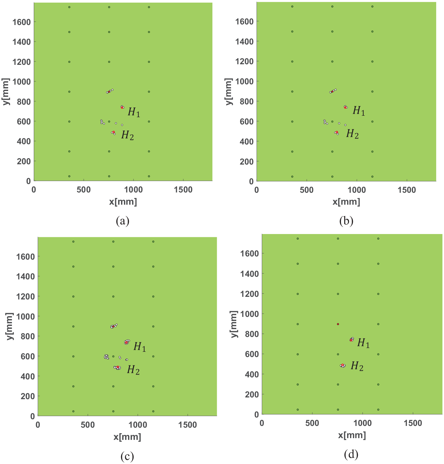
Imaging results of the experimental signal optimized intelligent defect location algorithm (a) g = 1, (b) g = 2, g = 3, and g = 4.
Conclusion
In this research, an improved intelligent defect location algorithm based on a helical guided wave was applied to the defect detection of a U-shaped boom. By combining the characteristics of an elliptic imaging algorithm, the algorithm improved the evolutionary algorithm and applied the K-means algorithm to population screening and population updating, which allowed it to retain the statistical characteristics of individuals and ensured the reliability of defect detection. First, the propagation characteristics of the helical guided waves in a U-shaped boom were analyzed, and the conclusion that the group velocity of the helical guided waves changed with the change of the wall thickness was obtained. Therefore, to improve the accuracy of the defect imaging, we proposed an optimization scheme to improve the intelligent defect location algorithm, fully consider the change of the group velocity of the helical guided waves, accurately calculate the arrival time of the initial individuals using the group velocity of different wall thicknesses, and accurately match the functional equation, Equation (7). Second, we verified the effectiveness of the improved intelligent defect location algorithm in the defect location algorithm through numerical simulation and experiments. When only one group velocity was considered, the improved intelligent defect location algorithm was in good agreement with the elliptical imaging algorithm. When the group velocities for different wall thicknesses were fully considered, the detection results of the optimized intelligent defect location algorithm had a higher resolution.
The current work of this paper is to accurately locate the artificial defects of a U-shaped boom under laboratory conditions. However, in real-world inspections, there are many interference factors in the defect detection process of a U-shaped boom that will significantly affect the detection and defect location results. For instance, the variation of the working environment temperature in the detection process could affect the ultrasonic velocity, resulting in defect positioning errors. Excessive noise may lead to the low signal-to-noise ratio of the detection signal, resulting in defects being missed. Problems such as the structural surface roughness caused by corrosion, progressive damage, or weld defects could also affect the propagation characteristics of ultrasonic waves and then affect the results of defect detection and location. In this research, only artificial defects were considered, but corrosion defects, progressive damage, or weld defects may occur in actual detection, which would produce more complicated signal processing difficulties and signal analysis problems. As a result, a more thorough study is required if the work of this paper is to be applied to the detection of real-world structures. In order to do so, it is important to move beyond the numerous interference issues stated above as well as some other potential challenges.
Footnotes
Declaration of conflicting interests
The author(s) declared no potential conflicts of interest with respect to the research, authorship, and/or publication of this article.
Funding
The author(s) disclosed receipt of the following financial support for the research, authorship, and/or publication of this article: This work was supported by the National Key R&D Program of China (nos. 2018YFC0809003 and 2018YFC1902400) and the National Natural Science Foundation of China (no. 11772014).