Damage evaluation and failure mechanism analysis of axially compressed circular concrete-filled steel tubular column via AE monitoring

Abstract

Concrete-filled steel tubular (CFST) columns are frequently used as the main load-bearing components in engineering structures due to their excellent load-bearing capacity. However, the presence of steel tube makes it impossible to accurately detect the damage characteristics of concrete by only relying on traditional mechanical measurement methods. This article quantitatively investigates the concrete damage of circular CFST column during axial compression based on the acoustic emission (AE) technique. Through the cumulative AE parameters including amplitude, count, and energy, the axial compression process of the CFST column can be divided into five main stages (Stage I is divided into two substages) to represent the different damage degree. The damage characteristics of concrete at each stage were explained by combining AE results and mechanical phenomena. A sensitivity analysis of the axial compression process was carried out using the Historic Index (HI) and Severity (Sr) and found that the sudden rise in HI and Sr corresponded to the changes in the different loading stages. The Improved b (Ib) value analysis calculated from the AE amplitudes reflects the evolution mechanism of the crack and can be used for the identification of the final failure moment of the specimen. Finally, a new method for processing and analyzing AE parameters was proposed, which effectively enhanced the dimensionality of real-time monitoring information on the damage of concrete filled in the steel tube.

Keywords

Concrete-filled steel tube acoustic emission axial compression damage characteristics

Introduction

Concrete-filled steel tubular (CFST) columns exhibit high load-bearing capacity, good ductility, excellent fire resistance, and ease of construction.^1,2 Due to these distinctive characteristics, CFST columns are increasingly being used as the main load-bearing members in challenging structures such as high-rise buildings,³ long-span bridges,⁴ deep underground tunnels,⁵ and offshore platforms.⁶ Failure of the main load-bearing components may lead to serious damage to the building structures or even total collapse. Currently, most of the existing studies rely on mechanical measurements and naked-eye observations to research the axial compression properties of the CFST columns.^7,8 However, the concrete could not be observed due to the presence of the outer steel tube, and the damage state of the concrete cannot be accurately monitored by strain gauges attached to the outer wall of the steel tube. A continuous monitoring of the damage state of the core concrete is necessary.

Acoustic emission (AE) is a transient stress wave phenomenon resulting from the rapid release of local energy when a material is deformed or subjected to external action.⁹ The AE monitoring technique determines the damage state of a material by recording, storing, and analyzing the stress waves generated at the location of the material damage.¹⁰ The AE signal contains information about the location, mechanism, and severity of the damage and is sensitive to minor damage, allowing monitoring not only of the damage state at the sensor location, but also of certain areas that are easily exposed to excited stress waves, without having to compromise the integrity of the structure.¹¹ Therefore, AE monitoring is a microanalysis and non-destructive testing method that is becoming increasingly attractive for use in civil engineering structures.

AE technique is widely used in the detecting and identifying the deteriorations of various engineering materials, including concrete,¹² asphalt,¹³ rock,¹⁴ mortar,¹⁵ etc. The research results indicate that AE signals are sensitive and effective for the generation, progression, and fracture of cracks in materials. It is also excellent in the research of the mechanical properties of various engineering components such as beams,¹⁶ slabs,¹⁷ columns,¹⁸ and joints.¹⁹ Due to its ability to detect the structures with large areas and many features, AE techniques are frequently used for damage assessment of bridge structures such as steel bridge,²⁰ concrete bridge,²¹ and masonry bridge.²²

The AE characteristics parameters, such as amplitude, counts, energy, and hits, extracted by analyzing the AE signal waves can be effectively used for the damage detection and classification of various materials. Wang et al.²³ divided the bonding behavior between rusted reinforcement and corroded concrete into four stages based on the variation trend of the number of AE events with time. Calabrese et al.²⁴ classified the process of stress corrosion cracking of precipitation-hardened martensitic stainless steel in chloride-containing environments according to the variation trend of cumulative AE counts with time. Li and Du²⁵ investigated the damage characteristics of ice structures under uniaxial compression and three-point bending test conditions. It was found that the axial compression process and bending process of the ice structure could be divided into the initial, stabilization, and failure stages according to the change in the cumulative AE energy rising rate with time.

It is difficult to assess the damage to the internal concrete of an in-filled concrete structure that cannot be directly observed and measured by conventional mechanical measurement methods. Several studies indicate that the AE technique is an effective means of detecting such structures.^18,26–29 Farhidzadeh et al.²⁶ proposed a probabilistic-based unsupervised pattern recognition algorithm to assess the soundness of the filled concrete in steel-concrete composite shear walls based on AE monitoring. Li et al.²⁷ confirmed that the AE technique can be used to detect sleeve grout compaction in fabricated shear wall. Du et al.²⁸ monitored the axial compression process of the steel tube confined reinforced-concrete columns (STCRC) using AE technique. The test results show that the AE technique is effective in assessing the damage state of STCRC columns, including identifying damage thresholds, revealing damage mechanisms, and classifying damage patterns. Li et al.²⁹ divided the uniaxial cyclic loading process of the fiber-reinforced plastic-confined circular CFST columns into three stages based on the AE signal analysis and proposed a modified damage index for quantitative evaluation of the damage degree of the specimens. Li et al.¹⁸ studied the bond-slip properties of the CFST columns by AE technique. However, relevant researches are lacking for the internal concrete damage assessment under axial compression of the circular CFST columns, which are widely used in engineering structures.

In this study, the axial compression test was carried out on the circular CFST column with the diameter of 1100 mm and AE monitoring was adopted to elucidate the entire damage process and analyze the damage characteristics. The mechanical properties of the specimen were measured and the force–strain curves were obtained. The typical cumulative AE parameters including amplitude, count, and energy were extracted to classify and refine the entire axial compression process of the CFST column. The comprehensive analysis of the loading process, Historic Index (HI), Severity (Sr), and Improved b (Ib) value, reveals the failure mechanism of the specimen and provides a critical warning. Finally, a new AE parameter Normalized Rise Angle (NRA) was proposed based on Rise Angle (RA), and then combined with HI to establish a new AE signal analysis method which reflects both real-time type and seriousness of crack while monitoring the crack development.

Experiment setup and AE analysis method

Specimen preparation

The specimen investigated in this study is the circular CFST column with a diameter (D) of 1100 mm. The height-to-diameter (H/D) ratio of the specimen is 2.5 to ensure short column and reduce the boundary effects. The diameter-to-thickness (D/t) ratio, cube concrete strength (size: 150 mm × 150 mm ×150 mm), and steel tube yield strength of 66.7, 59.22 MPa, and 267 MPa, respectively, meeting the limits of the prevailing codes such as EC4,³⁰ AIJ,³¹ AISC,³² and GB50936.³³ Where the concrete strength was obtained from six cube samples and six cylinder samples (size: 150 mm × 300 mm) cast from the same batch of concrete as the specimen and tested on the day when the specimen was loaded. Three tensile coupons were prepared and tested to determine the properties of the steel plate. The detailed parameters of the specimen are listed in Table 1.

Table 1.

Details of the tested specimen.

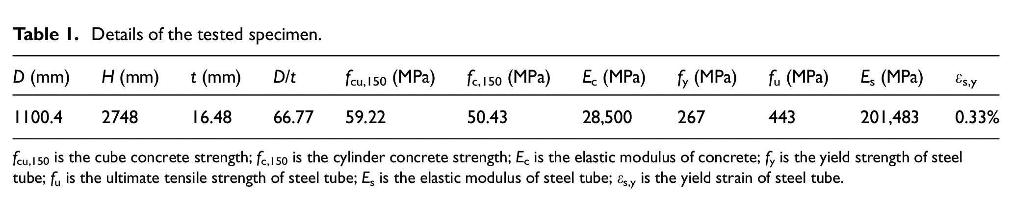
D (mm)	H (mm)	t (mm)	D/t	f _cu,150 (MPa)	f _c,150 (MPa)	E _c (MPa)	f _y (MPa)	f _u (MPa)	E _s (MPa)	ε _s,y
1100.4	2748	16.48	66.77	59.22	50.43	28,500	267	443	201,483	0.33%

f _cu,150 is the cube concrete strength; f_c,150 is the cylinder concrete strength; E_c is the elastic modulus of concrete; f_y is the yield strength of steel tube; f_u is the ultimate tensile strength of steel tube; E_s is the elastic modulus of steel tube; ε_s,y is the yield strain of steel tube.

Figure 1 shows that the specimen consists of a steel tube filled with concrete, 2 end plates, and 12 uniformly distributed stiffening ribs. The end plates were machined with a 2-mm-high circular table on Side A to avoid the direct loading on stiffening ribs, and a 2-mm-deep circular groove on Side B to facilitate the column positioning. The stiffening rib has the height (h_l) equal to one-tenth of the specimen’s height and the same thickness as the steel tube. The hollow steel tube was fabricated by rolling a 16 mm steel plate, the edges of which were machined to be flat to ensure uniform compression of the specimen. The bottom end plate was welded first to the hollow steel tube before concrete casting, followed by the welding of the top end plate. In addition, the surface of the column is leveled with high strength cement mortar prior to welding the top end plate. For more detailed fabrication process, refer to the tests of Liu et al.³⁴ and Gao et al.³⁵

Figure 1.

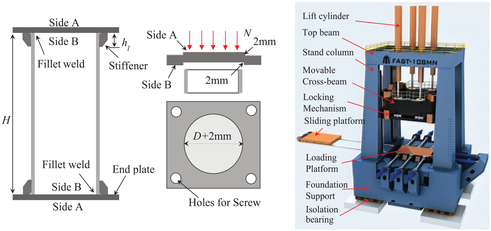
Schematic view and loading system of specimen.

Test setups and AE monitoring procedure

Eight displacement gauges with a range of 200 mm were arranged symmetrically on the specimen surface to measure the axial deformation of the specimen, four of them (type: LVDT) were used to measure the local displacement and the other four (type: YWD) were used to measure the overall displacement, as Figure 2(a) depicts. A series of strain gauges were arranged on the surface of the steel tube, with eight pairs symmetrically attached at the mid-height of the specimen and two pairs at the remaining height, each pair containing one transverse and one vertical, as shown in Figure 2(c).

Figure 2.

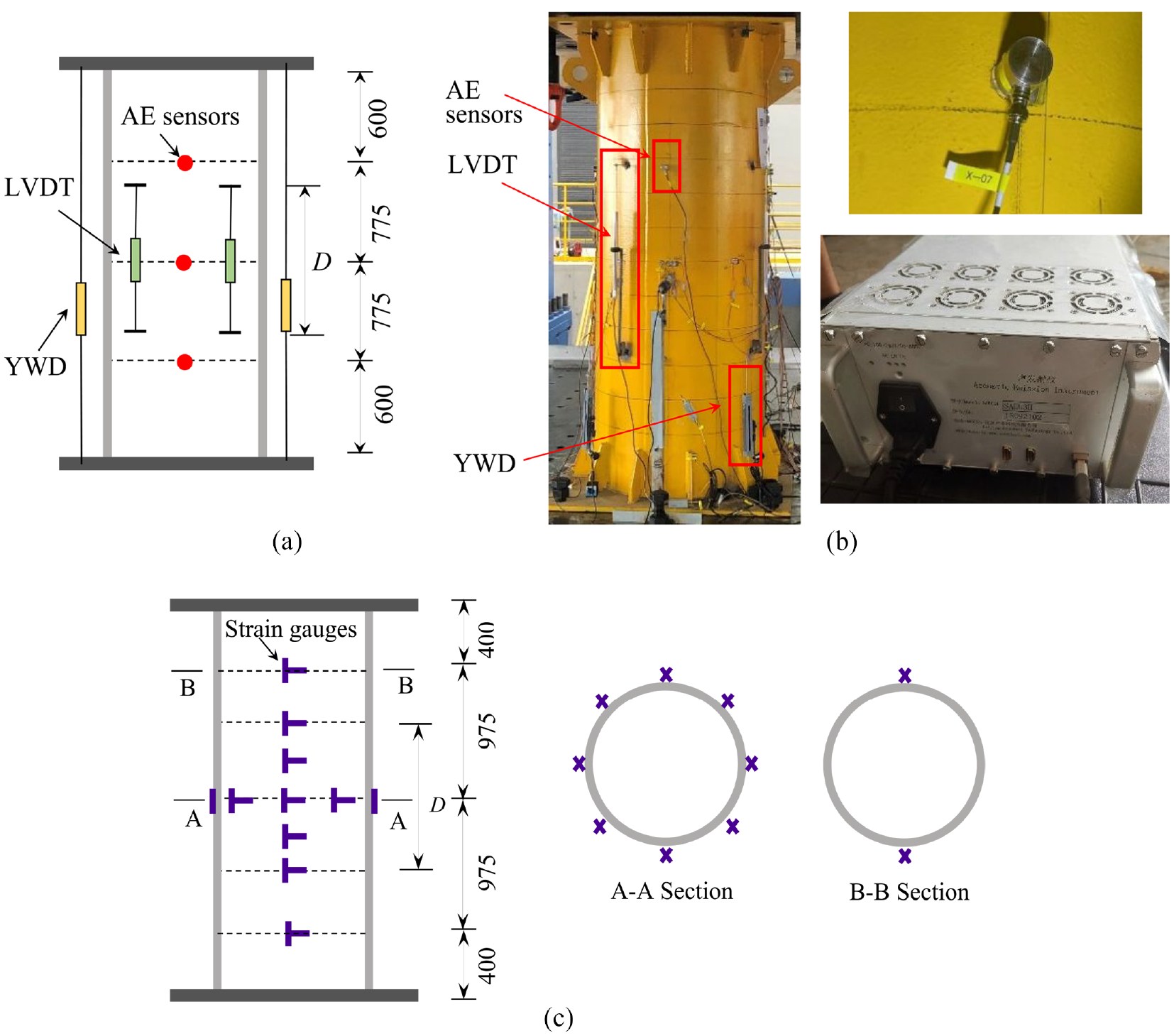
The arrangements of measuring instruments and acoustic emission (AE) sensors: (a) location of measurement points, (b) AE monitoring system, and (c) the arrangement of strain gauges.

The specimen was tested on a multifunctional loading system (Figure 1) at the China Construction Technology Centre in Beijing, which is able to apply a maximum axial force of 108 MN. The specimen was loaded using load or displacement control. Before the specimen reached its expected peak strength (N_u,cal) based on the EC4,²⁷ a load-controlled loading with 5% N_u,cal increments was adopted, where the loading rate was set as 0.03 MPa/s when the applied load was less than 60% N_u, after which the loading rate was adjusted to 0.02 MPa/s. After the peak strength (N_u,exp), a displacement-controlled loading at a rate of 0.1 mm/s (the minimum loading rate of the system) was used until the specimen failed.

A multi-channel AE data acquisition and analysis system manufactured by Soundwel Science & Technology Co., Ltd., Beijing, China, was adopted to acquire the AE signals emitted during the axial compression process, as shown in Figure 2(b). The pre-amplifier with a gain of 40 dB was used to pre-amplify the AE signals. A personal computer was used to store real-time AE signals. In all, 12 AE sensors of SR 150M with frequency bands ranging from 60 to 400 kHz were attached to the specimen surface using hot glue, the position of the AE sensors is shown in Figure 2(a) with three layers, and four in each layer arranged symmetrically. The sensor output voltage value of 1 µV corresponds to a recorded 0 dB. Prior to loading the specimen, a pencil break test was carried out to ensure the effectiveness of the hot glue fastened the AE sensors. The threshold of the AE collection system was set as 45 dB to filter out ambient noise. The low- and high-pass frequency were set as 20 and 400 kHz, respectively. The sampling frequency is 5000 kHz. The channel acquisition parameters were determined according to the properties of the concrete material. The peak definition time, hit definition time, and hit lockout time for these sensors were set as 50, 150, and 300 μs, respectively.

AE characteristic parameters

The characteristic parameters of AE such as amplitude, hit, count, duration, rise time, and energy could be extracted by analyzing the AE signal waveform, which reflects the features of the damage source. Figure 3 shows a typical waveform schematic and the definition of each parameter. Where energy is the area under the signal waveform, calculated according to Equation (1). The hits are the number of oscillations in the signal waveform that exceed the threshold (45 dB), and one “hit” is represented in Figure 3.

Energy = \int_{0}^{t} V^{2} (t) d t

(1)

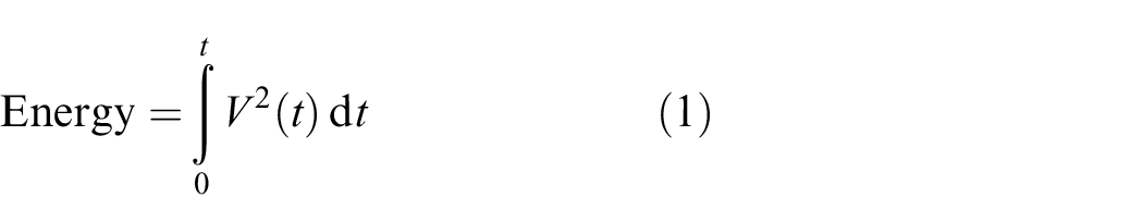
Note: V(t) is the recorded voltage; t is the duration time.

Figure 3.

Acoustic emission (AE) signal and parameters.¹²

Results and discussion

Mechanical behaviors

Figure 4 plots the load–strain curve and the load ratio–Poisson’s ratio curve of the specimen. The strains (ε_exp) are determined according to the local displacements measured by the LVDTs before 60% N_u,exp to avoid the virtual displacement induced by the uneven end plate in the initial loading stage and the overall displacement measured by the YWDs after 60% N_u,exp to consider the local softening of the specimens.³⁶ Based on the load–strain curve, the axial compression performance of CFST column can be divided into four stages: (I) elastic stage, (II) elastic–plastic stage, (III) strain hardening stage, and (IV) falling stage. This coincides with the results of experimental studies by Han et al.³⁷ and Wang and Zhang.³⁸

Figure 4.

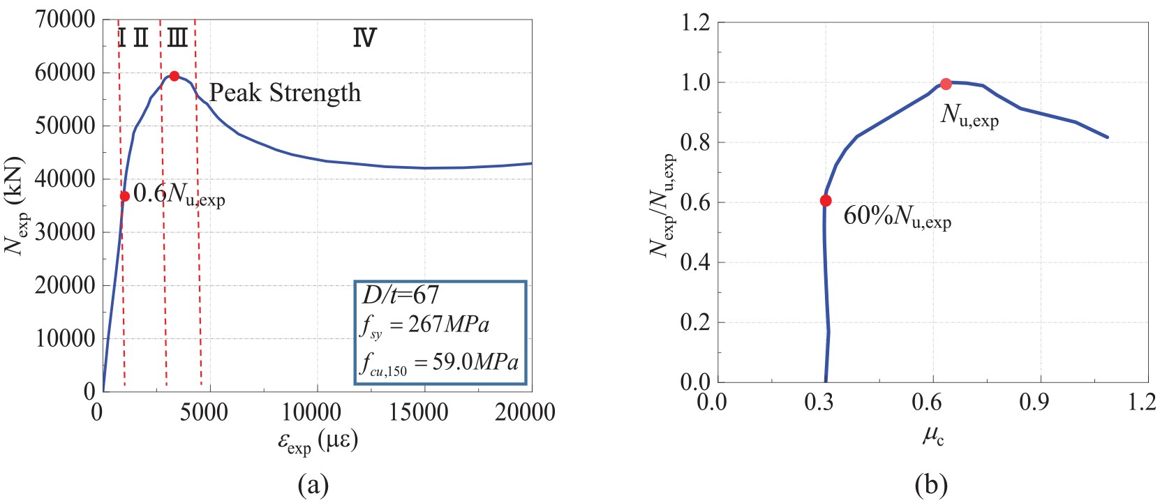
The vertical strain and Poisson’s ratio curves: (a) load versus axial strain curve and (b) load ratio versus Poisson’s ratio curve.

In the initial stage of loading, the load increases uniformly, the Poisson’s ratio was stable at about 0.3 (Poisson’s ratio of steel), and there was no obvious change in the surface of the specimen, indicating that the steel tube and concrete were in the state of independent work during this period. The rising rate of the loads started to reduce at 0.6 N_u,exp and the Poisson’s ratio increased rapidly with the load, which means that the transverse deformation of the steel tube increased faster and the specimen from the elastic stage (I) into the elastic–plastic stage (II). The specimen entered the strain hardening stage (III) near the peak point, during this period the load-bearing capacity of the specimen remained around the peak strength and the Poisson’s ratio increased at a further accelerated rate. However, the boundaries of this stage are ambiguous. The peak strength of the specimen was measured to be 59,361 kN and the peak strain to be 3197 με. Thereafter, the load-bearing capacity of the specimen dropped rapidly, and when it decreased to about 0.85 N_u,exp, the obvious local buckling occurred on the upper north and lower south sides of the steel tube and the specimen failed (Stage IV).

The variation of the strains measured by all strain gauges with the increasing load is shown in Figure 5. Define the compressive strain as negative and the tensile strain as positive. Some new key points could be identified from this figure. Since the surface of the steel tube did not show significant buckling before the specimen reached the ultimate bearing capacity, the steel tube can be considered to be in close contact with the concrete and without slippage. The strain on the outer surface of the steel tube could be used to represent the strain of the concrete. The concrete reached the failure strain ( $ε'_{cu}$ ) when the load-bearing capacity of the specimen reached 0.73 N_u,exp. The failure strain is defined by Equation (2),³⁹ which is based on Equation (4)⁴⁰ and considers the influence of size. The vertical and hoop strains reached the yield strain (ε_sy) of the steel tube at 0.90 N_u,exp and the peak point, respectively.

ε'_{cu} = (1.4 γ_{u} - 0.4) \times ε_{cu}

(2)

γ_{u} = \frac{0.7}{\sqrt{1 + 0.017 D}} + 0.63

(3)

ε_{cu} = 700 + 172 \sqrt{f_{c}}

(4)

Note: ε_cu is the failure strain of standard concrete sample.

Figure 5.

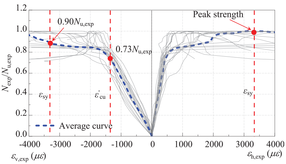
The curves of load ratio versus strains obtained from strain gauges.

It is worth noting that it is difficult to determine exactly the moment when a through crack was formed in the internal concrete, that is, the time of specimen failure, by visual observation of the specimen surface alone. Also the damage characteristics and evolutionary behaviors of the core concrete at different loading levels cannot be quantitatively evaluated. Therefore, AE monitoring system is required to detect the damage of the concrete. The final failure pattern of the specimen is shown in Figure 6. None of the welds cracked during the loading process and none of the ends of the specimen buckled.

Figure 6.

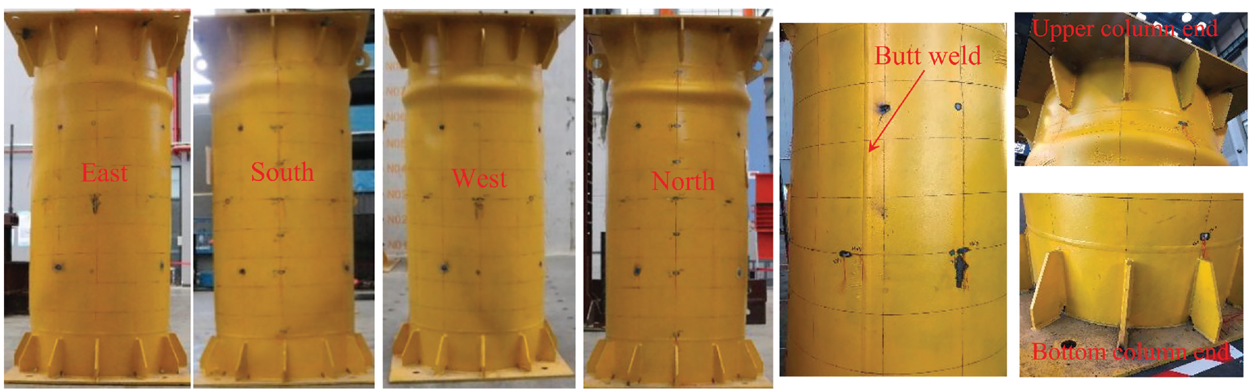
Final failure mode.

Damage classification

AE is a real-time, non-damage detection technique that reflects the different forms of damage resulting from the deterioration of materials under stress. In this section, besides cumulative amplitude, the efficiency of other AE parameters in assessing the damage progression of the CFST column is demonstrated.

Cumulative AE parameters

The evolution of the normalized cumulative AE parameters, such as count, duration, energy, etc., with the increasing load is shown in Figure 7. Define 5% N_u,exp as a load step. These cumulative AE parameters increase gradually with the increasing load, similar to the trend of the axial strain. However, the rising rate of the cumulative AE parameters under different load levels differed significantly compared to the strain. Except for energy, these cumulative AE parameters including amplitude, count, etc. rise with the increasing load in a similar manner. The cumulative AE parameters rise slowly at a uniform rate at the beginning, then slow down after two obvious accelerations of the rising rate, and finally rise sharply. Each obvious change in the rising rate of the cumulative parameters reflects the different stress stages of the CFST column under axial compression. Therefore, the axial compression process of the specimen could be refined into five main stages based on the evolution of these cumulative AE parameters. This differs from the results divided by mechanical curve. The AE energy curve differs from the rest of the cumulative AE parameter curves, by not identifying the boundary between Stage I and Stage II. Therefore, the ability of the AE parameters to subdivide the axial compression process of the CFST column is presented using the amplitude as an example. In addition, the substages of the Stage I division in Figure 7 are described in Section “AE signal intensity analysis.”

Figure 7.

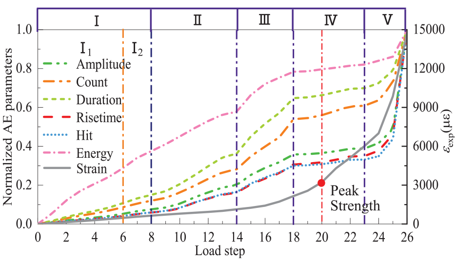
Relationships between normalized acoustic emission (AE) parameters and load step.

Cumulative AE amplitude

Figure 8 shows the normalized cumulative AE amplitude and strain verses load step curves. In Stage I, the cumulative AE amplitude rose with a slow and uniform rate. During this stage, the AE events originated from the initiation and propagation of microcracks that appeared at the initial internal defects (the stress concentration areas) of the concrete. Stage II began at N_exp = 0.4 N_u,exp (point A) and closely related to the further initiation and propagation of microcracks. Point B (0.7 N_u,exp) was used as the demarcation point between Stage II and III and may be associated with the strain of the concrete reaching its failing strain (Figure 5). Indicating that Stage II before point B was the unstable propagation stage of microcracks in concrete, and after the concrete reached its failure strain at point B, the microcracks started to penetrate locally to form macrocracks at Stage III. The most noteworthy Stage IV began when the load-bearing capacity of the specimen reached 0.9 N_u,exp (point C), and ended when the residual load-bearing capacity was 0.85 N_u,exp (point D). Point C coincided well with the moment when the vertical strain of the steel tube reached its yield strain (Figure 5). In Stage IV, the curve rose slowly, different from the fast-rising trend of the previous two stages. Indicating that during this stage, the additional load was more borne by the concrete part, the lateral deformation of concrete was intensified, and the steel tube played an effective confining role on the concrete, which confined the propagation of concrete cracks. And due to the confining effect of the steel tube, there was no significant abrupt change in the cumulative AE amplitude when the specimen reached its peak strength. It was observed during the test that significant buckling of the specimen began to occur on both the upper north side and the lower south side of the specimen when the bearing capacity dropped to 0.85 N_u,exp (point D). This implied that the main crack in the specimen had formed before this point and that the specimen slid staggered along the shear surface after this point.⁴¹ Therefore, Stage IV was the forming stage of main crack and Stage V was the failure stage (a shear plane was formed along the main crack and the dislocation occurred along the shear plane). Furthermore, due to the large amount of AE signals emitted by the frictional sliding of concrete along the shear surface, the cumulative AE parameters rose sharply in Stage V.

Figure 8.

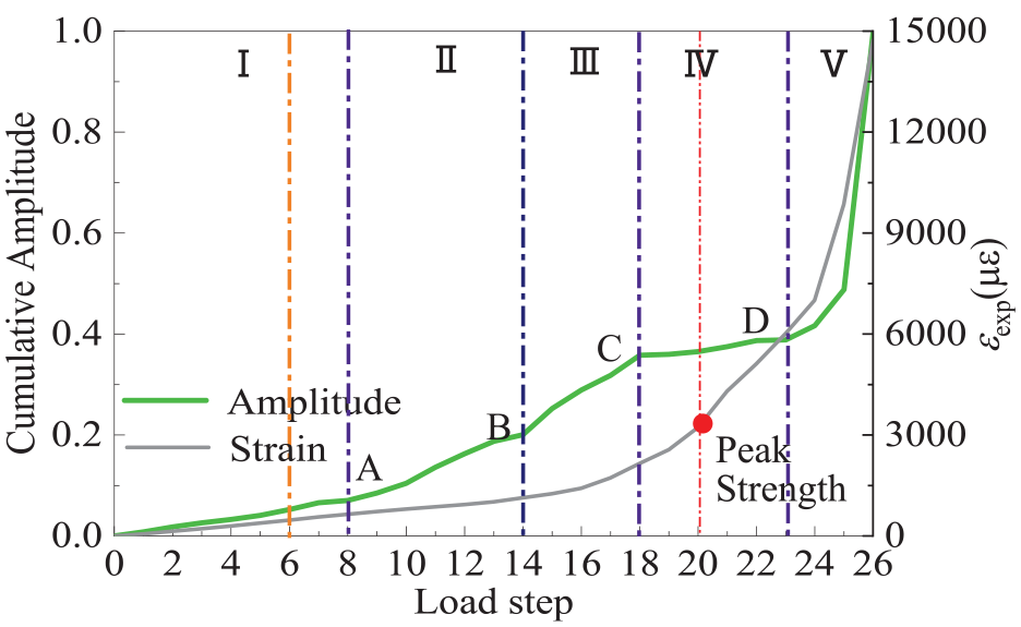
Normalized acoustic emission (AE) cumulative amplitude and strain versus load step.

In conclusion, as shown in Figure 7, the axial compression process of the CFST column can be divided into five main stages according to the change in the rising rate of the accumulative AE parameters: (I) microcrack initiation and propagation stage, (II) microcrack in unstable progression stage, (III) microcrack local penetration stage, (IV) main crack formation stage, and (V) failure stage.

AE signal intensity analysis

A series of AE parameters such as amplitude, count, and energy can be used to characterize the intensity of the AE signals, with the energy being the most used.⁹ The HI and Sr are both calculated according to energy, and are effective parameters for evaluating the damage degree of the specimen.^12,42

The HI reflects the real-time variation of the AE signal, determined by Equation (5), and is able to record any sudden changes in the intensity of the accumulative AE signal.⁴²

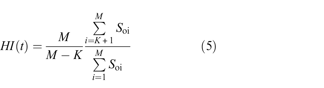
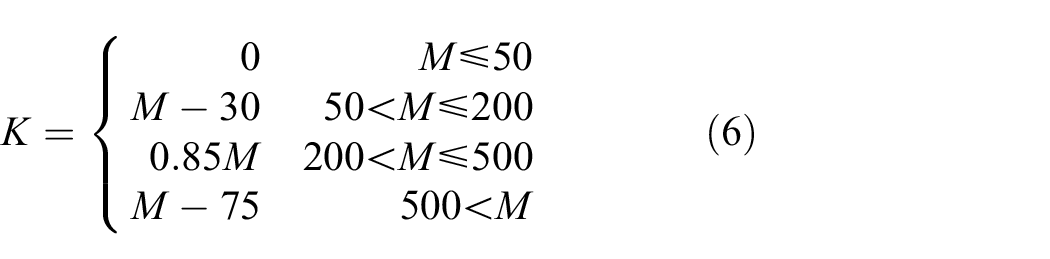
HI (t) = \frac{M}{M - K} \frac{\sum_{i = K + 1}^{M} S_{oi}}{\sum_{i = 1}^{M} S_{oi}}

(5)

where H(t) is the Historic Index at time t; M is the number of hits up to and including time t; S_oi is the strength of the collected AE signals arranged in a time sequence; K is a constant defined by the number of collected AE signals and the type of material, determined by Equation (6).

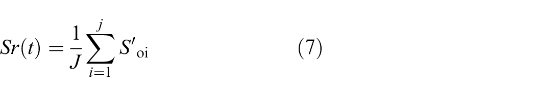
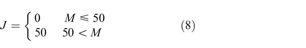
K = {\begin{matrix} 0 & M \leq 50 \\ M - 30 & 50 < M \leq 200 \\ 0.85 M & 200 < M \leq 500 \\ M - 75 & 500 < M \end{matrix}

(6)

Sr is defined as the average of J consecutive AE signals with maximum energy. It can be used to characterize the variation of the strong AE signal and is calculated as Equation (7).

Sr (t) = \frac{1}{J} \sum_{i = 1}^{j} {S'}_{oi}

(7)

where $S'_{oi}$ is the average signal of the J largest signal strengths of the collected AE signals; J is the empirical parameter determined by the type of material, as shown in Equation (8).

J = {\begin{matrix} 0 M \leq 50 \\ 50 50 < M \end{matrix}

(8)

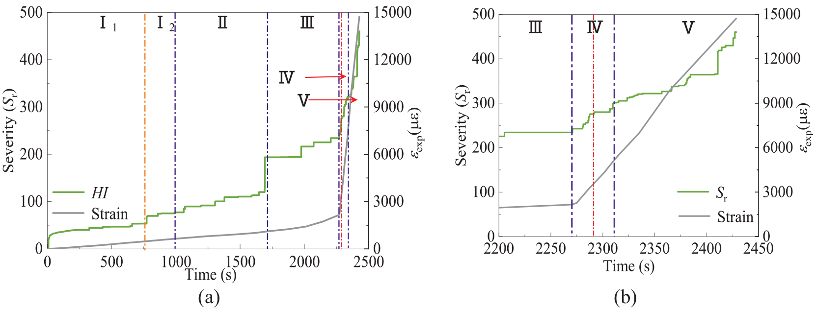
The variations of HI and the axial strain of the specimen with time are shown in Figure 9, where the loading stage is indicated. It should be noted that the abrupt changes in HI and the division of the loading stages according to the cumulative AE parameters are well fitted. During Stage I, HI started with a slight fluctuation around 1.00, rose abruptly to 1.95 at 770 s (N_exp = 0.3 N_u,exp), and then continued to fluctuate with a slightly larger range around 1.00. The first sudden rise in HI may be closely related to the first cracking of the concrete, using this as a boundary to divide the first stage into two substages: (I₁) before the cracking of the concrete, that is, the coalescence stage of the microcracks, and (I₂) after the cracking of the concrete, that is, the initiation and progression of the microcracks.

Figure 9.

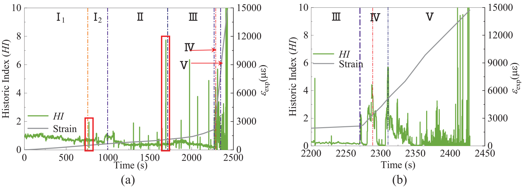
Variations in Historic Index (HI): (a) Stages I–V and (b) Stages III–V.

After entering Stage II, HI experienced several sudden rises with values within 2.00. Then, HI suddenly rose to 7.73 at 1690 s (as shown in the second red box, which was the strongest AE signal appeared before the peak load), at which point Stage II was finished, corresponding to the strain of the concrete reaching its failing strain. The abrupt rises of HI occurred more frequently in Stage III than in II and these rises were also significantly greater. It is clear from Figure 9(b) the three peaks of HI in Stage IV coincide with the end of Stage III, the peak strength of the specimen and the end of Stage IV, respectively. Furthermore, these three peaks increase in sequence, being 2.26, 4.47, and 5.69, respectively. In addition, the consecutive high HI values presented after the generation of the main crack (at the end of the Stage IV) during 2400–2428 s may be attributed to the formation of the shear plane and dislocation of the specimen along the shear plane. Figure 10 shows that the jump up in S_r occurs at the same moment as the sudden rise in HI. Therefore, both S_r and HI could be used to monitor the axial compression process of CFST column in real time.

Figure 10.

Variations in Severity (Sr): (a) Stages I–V and (b) Stages III–V.

Crack evolution

The b value analysis was originally applied to seismic wave analysis in earthquakes, reflecting the relationship between the magnitude and frequency, as shown in Equation (9).⁴³

\log_{10}^{N} = a - b M_{L}

(9)

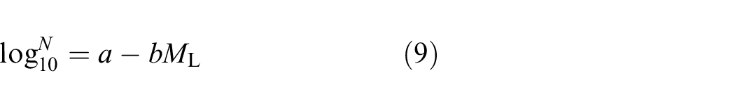
where M_L is the Richter magnitude of the seismic event; N is the incremental frequency (the number of seismic events with magnitude increment ΔM_L); a and b are empirical constants. Recently, this method has been used to analyze AE signals.¹³ However, this method only considers large amplitude AE signals and ignores the small amplitude signals which also holds energy. Therefore, an Ib value method was used to analyze the cracking process of concrete as shown in Equation (10).¹⁷

Ib = \frac{\log N (μ - α_{1} σ) - \log N (μ + α_{2} σ)}{(α_{1} + α_{2}) σ}

(10)

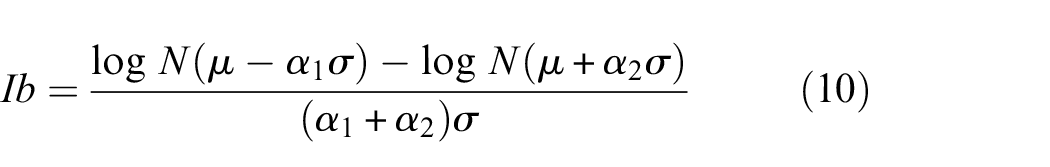
where μ and σ are the average and standard deviation of AE amplitudes, respectively; N (μ − α₁σ) and N (μ + α₂σ) are the number of the AE signals with amplitudes greater than (μ − α₁σ) and (μ + α₂σ), respectively; α₁ and α₂ are empirical constants set as 0 and 1, respectively. The changes in Ib value reflect the development of cracks within the material. The Ib value rises during the nucleation of the microcracks and drops during the coalescence of the microcracks and macrocracks.⁴⁴

Figure 11 shows the variation of Ib values calculated from the AE signals collected during the axial compression of the CFST column with the increasing load step. As can be seen, three groups of Ib values are shown and the numbers indicate the number of AE signals (N) used to calculated the Ib value. To clarify the effect of the group size of the AE signals on which the calculation was based, the influence on the Ib value was discussed for N = 50, 100, and 200. In Stage I and II, the magnitude of the Ib values is influenced by the value of N taken, while the trend of change is not affected. In Stage III and IV, the Ib value curves are almost the same for different N. Therefore, the Ib values calculated based on groups containing between 50 and 200 signals could all be used to analyze the axial compression process of CFST column. The Ib value curve with N = 100 is discussed below as an example to illustrate the variation of the Ib values under different load stages.

Figure 11.

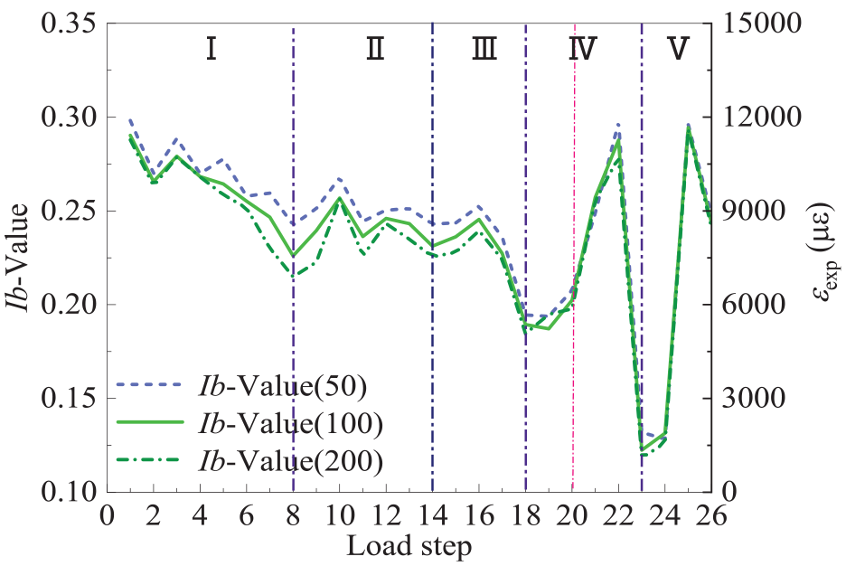
Variations of Improved b (Ib) values.

At the boundary of each stage, the Ib value curve is at a trough, indicating that the Ib value curve reflects the damage degree of core concrete effectively. There are a total of three distinct troughs in the Ib value curve, with progressively lower Ib values at the troughs, showing increasingly severe damage to the concrete. The Ib value curve kept fluctuating down in the first stage and reached the first trough of 0.226 at the eighth load step, corresponding to the initiation and propagation of microcracks. In Stage II, the Ib values decreased fluctuatingly, corresponding to the continuous progression of microcracks. The second trough was reached at the end of the Stage III with a Ib value of 0.189, when the vertical strain of the steel tube reached its yield strain. The curves rose rapidly and then fell sharply in the Stage IV, reaching the third trough at the end of these stage with a Ib value of 0.122, which was much lower than the previous two. This implied the formation of a large penetrating fracture. In Stage V, the curves rose again, indicating that some new cracks were in the sprouting stage, but by this time the specimen had failed.

Crack classification

The combined parametric analysis method based on RA and AF (Average Frequency) is effective in revealing the progression of cracks in concrete-related materials and is used to qualitatively distinguish between types of cracks.²⁸RA is the ratio of rise time and amplitude of an AE signal (Equation (11)), and AF is the ratio of count and duration (Equation (12)).

Rise Angle (RA) = \frac{Rise Time}{Amplitude}

(11)

Average Frequency (AF) = \frac{Counts}{Duration Time}

(12)

Figure 12 shows the crack modes of the concrete including tensile cracks, shear cracks, and the corresponding AE characteristics of each crack mode. During crack formation, tensile cracks emit longitudinal waves, while shear cracks emit transverse waves.¹⁷ As longitudinal waves propagate faster in solid materials, the tensile cracks take less time to reach maximum amplitude than the shear cracks. According to Equations (11) and (12), the tensile cracks exhibit smaller RA values and larger AF, while the opposite is true for the shear cracks. However, the information on the intensity of the injury source is lost by relying on RA-AF analysis alone. Previous studies have conducted both separately, resulting in incomplete and missing information on crack damage. In addition, the RA-AF analysis is conducted based on rise time, amplitude, count, and duration except energy parameter. While the HI analysis is obtained from the AE energy calculation. Therefore, the analysis method combining RA-AF and HI is needed and adopted in this study to investigate the axial compression processes of CFST column. Since the RA values and AF are approximately inversely related and a standard ratio is missing between RA values and AF according to related researches,⁴⁵ independent analysis of RA values is similar to the analysis of RA-AF. The RA values are normalized according to Equation (13).

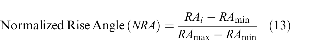
Normalized Rise Angle (NRA) = \frac{R A_{i} - R A_{min}}{R A_{max} - R A_{min}}

(13)

where RA_i is the RA value recorded in real time; RA_min and RA_max are the maximum and minimum RA values, respectively. The AE signal tends to be from a shear crack when the NRA values is close to 1.00 and from a tensile crack when the NRA value is close to 0.00.

Figure 12.

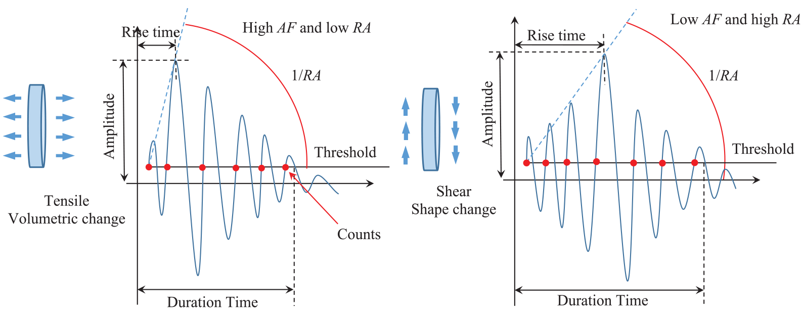
The corresponding acoustic emission (AE) characteristics of crack modes.¹⁷

Figure 13 shows the AE signal sequence with crack modes and intensity information.

Figure 13.

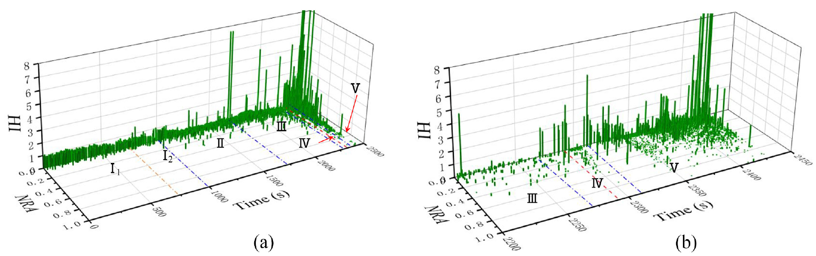
The acoustic emission (AE) signal sequence with crack modes and intensity information: (a) Stages I–V and (b) Stages III–V.

During Stage I₁, the NRA values for all AE signals were less than 0.10 and the HI values were less than 1.00, indicating that all the microcracks produced at this stage were low-intensity tensile cracks . The NRA values of the signals in Stage I₂ were still all less than 0.10, but several signals with 1.00 < HI < 2.00 appeared. In Stage II, cracks with low intensity (HI < 1.00) that tend to be in shear mode (NRA < 0.4) began to emerge. However, those several signals with high intensity (at the end of Stage II) indicating that the concrete had reached its failing strain still originated from tensile cracks. A greater number of cracks tending to shear mode occurred in Stage III, but the HI for such cracks in this stage was still less than 1.00. The cracks of higher intensity (HI = 3.52) tending to shear mode were first observed near the peak strength of the specimen. After entering Stage V, shear cracks dominated, meaning that although the cracks generated during the axial compression of the CFST column were dominated by tensile cracks, the failure of the column was originated from the generation of shear cracks.

Conclusion

The axial compression process of the circular CFST column was monitored using the AE method. The damage stages were classified according to the change in the slope of the cumulative AE parameter curves. Based on the AE intensity analysis and the Ib values, the damage characteristics of the core concrete during axial compression were discussed. The types of cracks were discussed by combining the NRA values with the HI. The following conclusions can be drawn:

The rising ratio of the cumulative AE parameters including amplitude, count, and hit varies significantly with the progression of the cracks, which reflects and characterizes the detailed damage process and mechanism of the CFST column under axial compression.

The damage degrees of the core concrete during the axial compression can be classified and identified according to the slope changes of the cumulative AE parameters. The axial compression process of CFST column can be divided into five main stages: (I) microcrack initiation and progression stage, (II) microcrack in unstable progression stage, (III) microcrack local penetration stage, (IV) main crack formation stage, and (V) failure stage. Furthermore, the Stage I is divided into two substages: (I₁) microcrack coalescence stage and (I₂) microcrack initiation and progression stage, with the division point corresponding to the moment of first cracking of the concrete.

The HI and Sr are sensitive to the core concrete damage and their sudden rise is consistent with the classification of the loading stage.

The Ib value clearly identifies the stage from microcrack initiation to the main crack formation and could determine the specimen failure more effectively.

The analysis method combining RA values with HI analysis for monitoring the concrete damage processes is effective in reflecting the intensity and type of cracks. The AE signal is dominated by low intensity (HI < 2.00) tensile-type cracks until the peak strength of the specimen is reached. The appearance of shear-type cracks with higher intensity indicates that the specimen is about to reach the peak strength. The failure of the specimen is closely related to the shear-type cracks with higher intensity (HI > 2.00).

Footnotes

Acknowledgements

Thanks to the editor and several reviewers for their efforts to improve and correct this article. Since some comments suggested by the reviewers were very meaningful and could not be fully reflected in the article, a link is provided to help readers read the full “response to reviewers.”

Declaration of conflicting interests

The author(s) declared no potential conflicts of interest with respect to the research, authorship, and/or publication of this article.

Funding

The author(s) disclosed receipt of the following financial support for the research, authorship, and/or publication of this article: This research is financially supported by the National Natural Science Foundation of China (Grant Number: U20A20312), which is gratefully acknowledged.

ORCID iDs

Yubo Jiao

Wenchen Shan

References

Han

Yao

. Experimental behavior of thin-walled hollow structural steel (HSS) columns filled with self-consolidating concrete (SCC). Thin-Walled Struct 2004; 42: 1357–1377.

Yang

Gao

, et al. Practical formular for predicting axial strength of circular-CFST columns considering size effects. J Constr Steel Res 2020; 168: 105979.

Giakoumelis

Lam

. Axial capacity of circular concrete-filled tube columns. J Constr Steel Res 2004; 60: 1049–1068.

Brown

Kowalsky

Nau

. Impact of D/t on seismic behavior of reinforced concrete filled steel tubes. J Constr Steel Res 2015; 107: 111–123.

Chang

Luo

Zhu

, et al. Analysis of circular concrete-filled steel tube (CFT) support in high ground stress conditions. Tunnelling Underground Space Technol 2014; 43: 41–48.

Hasan

Ekmekyapar

Shehab

. Mechanical performances of stiffened and reinforced concrete-filled steel tubes under axial compression. Mar Struct 2019; 65: 417–432.

Ekmekyapar

AL-Eliwi

BJM

. Experimental behaviour of circular concrete filled steel tube columns and design specifications. Thin-Walled Struct 2016; 105: 220–230.

Zhou

Sun

. Impact of D/t ratio on circular concrete-filled high-strength steel tubular stub columns under axial compression. Thin-Walled Struct 2018; 132: 461–474.

Behnia

Chai

Yorikawa

, et al. Integrated non-destructive assessment of concrete structures under flexure by acoustic emission and travel time tomography. Constr Build Mater 2014; 67: 202–215.

10.

Zhang

Shan

Zhang

, et al. AE monitoring of reinforced concrete squat wall subjected to cyclic loading with information entropy-based analysis. Eng Struct 2018; 165: 359–367.

11.

Philippidis

Assimakopoulou

. Using acoustic emission to assess shear strength degradation in FRP composites due to constant and variable amplitude fatigue loading. Compos Sci Technol 2008; 68: 840–847.

12.

Shan

Liu

Ding

, et al. Assessment of bond-slip behavior of hybrid reinforced engineered cementitious composites (ECC) and deformed rebar via AE monitoring. Cem Concr Compos 2021; 118: 103961.

13.

Jiao

Shan

, et al. Damage fracture characterization of pervious asphalt considering temperature effect based on acoustic emission parameters. Eng Fract Mech 2019; 210: 147–159.

14.

Lei

Masuda

Nishizawa

, et al. Detailed analysis of acoustic emission activity during catastrophic fracture of faults in rock. J Struct Geol 2004; 26(2): 247–258.

15.

Wang

Chen

, et al. Damage processes of steel fiber reinforced mortar in different fiber content revealed by acoustic emission behavior. Russ J Nondestr Test 2018; 54(1): 55–64.

16.

Shahidan

Pulin

Bunnori

, et al. Damage classification in reinforced concrete beam by acoustic emission signal analysis. Constr Build Mater 2013; 45: 78–86.

17.

Shan

Liu

, et al. Characterization of damage on precast pre-stressed concrete composite slabs under static loading based on acoustic emission parameters. Struct Health Monit 2020; 19(6): 2091–2106.

18.

Liu

Zhang

. Non-linear distributions of bond-slip behavior in concrete-filled steel tubes by the acoustic emission technique. Structures 2020; 28: 2311–2320.

19.

Benavent-Climent

Castro

Gallego

. AE monitoring for damage assessment of RC exterior beam-column sub assemblages subjected to cyclic loading. Struct Health Monit 2009; 8(2): 175–189.

20.

Alavi

Hasni

Jiao

, et al. Fatigue cracking detection in steel bridge girders through a self-powered sensing concept. J Constr Steel Res 2017; 128: 19–38.

21.

Anay

Cortez

Jauregui

, et al. On-site acoustic-emission monitoring for assessment of a prestressed concrete double-tee-beam bridge without plans. J Perform Constr Facil 2016; 30(4): 04015062.

22.

Han

Carpinteri

, et al. Localization of acoustic emission sources in structural health monitoring of masonry bridge. Struct Contr Health Monit 2015; 22(2): 314–329.

23.

Wang

Xia

, et al. Experimental study of a pull-out test of corroded steel and concrete using the acoustic emission monitoring method. Constr Build Mater 2016; 122: 163–170.

24.

Calabrese

Bonaccorsi

Proverbio

, et al. SCC damage evolution on martensitic stainless steel by using acoustic emission technique. Corros Eng Sci Technol 2015; 50(5): 1743–2782.

25.

. Monitoring and evaluating the failure behavior of ice structure using the acoustic emission technique. Cold Reg Sci Technol 2016; 129: 51–59.

26.

Farhidzadeh

Epackachi

Salamone

, et al. Bayesian decision and mixture models for AE monitoring of steel-concrete composite shear walls. Smart Mater Struct 2015; 24: 115028.

27.

Liu

, et al. Influence of grouted sleeve and concrete strength of fabricated shear wall on acoustic emission detection method for sleeve compactness. J Build Eng 2021; 43: 102541.

28.

Pan

. Damage evaluation and failure mechanism analysis of steel tube confined reinforced-concrete columns by acoustic emission technology. Lat Am J Solids Struct 2018; 15(11): e136.

29.

. Damage evaluation of fiber reinforced plastic-confined circular concrete-filled steel tubular columns under cyclic loading using the acoustic emission technique. Smart Mater Struct 2017; 26: 035014.

30.

EN 1994-1-1:2009. Design of composite steel and concrete structures—Part 1-1: General rules and rules for buildings.

31.

AIJ:2008. Recommendations for design and construction of concrete filled steel tubular structures.

32.

AISC360-10:2010. Specification for structural steel buildings.

33.

GB50936:2014. Technical code for concrete filled steel tubular structures.

34.

Liu

Gao

Lin

, et al. Experimental assessment on the size effects of circular concrete-filled steel tubular columns under axial compression. Eng Struct 2023; 275: 115247.

35.

Gao

Zhou

Liu

, et al. Experimental assessment on the size effects of square concrete-filled steel tubular columns under axial compression. Eng Struct 2023; 281: 115706.

36.

Teng

. Cyclic lateral response of FRP-confined circular concrete-filled steel tubular columns. J Constr Steel Res 2016; 124: 12–22.

37.

Han

Yao

Zhao

. Tests and calculations for hollow structural steel (HSS) stub columns filled with self-consolidating concrete (SCC). J Constr Steel Res 2005; 61(9): 1241–1269.

38.

Wang

Zhang

. Experimental research on axially loaded high-strength concrete-filled steel tubes. J Harbin Inst Technol 2004; 36(12): 1646–1648, 1685.

39.

Chen

Wang

Zhang

. Size effect prediction on axial compression strength of circular CFST columns. J Constr Steel Res 2020; 172: 106221.

40.

Guo

. Strength and principal structure relationships of concrete: principles and applications. Beijing: China Construction Industry Press, 2004 (in Chinese).

41.

Cai

Jiao

. Behavior and ultimate strength of short concrete-filled steel tubular columns. J Build Struct 1984; 5(6): 13–29.

42.

Chen

Feng

, et al. Damage analysis of CFRP-confined circular concrete-filled steel tubular columns by acoustic emission techniques. Smart Mater Struct 2015; 24(8): 085017.

43.

Gutenberg

Richter

. Seismicity of the earth and associated phenomena. J Geophys Res 1950; 55(1): 97–98.

44.

Farhidzadeh

Salamone

Luna

, et al. Acoustic emission monitoring of a reinforced concrete shear wall by b-value-based outlier analysis. Struct Health Monit 2013; 12(1): 3–13.

45.

Abouhussien

Hassan

AAA

. Assessment of crack development in engineered cementitious composites based on analysis of acoustic emissions. J Mater Civ Eng 2019; 31(6): 04019078.