Structural temperature gradient evaluation based on bridge monitoring data extended by historical meteorological data

Abstract

The structural temperature gradient (STG) is one of the most key factors causing cracking and even damage to bridge structures. However, its real effects on bridge structures are often over- or underestimated in practice. For most operating bridges, the structural health monitoring systems have just been put into use recently, and the monitoring structural temperature data are limited, which always leads to unreasonable STG representative value for a long return period based on such short-term structural temperature data. To solve the problems, this article proposes an STG determination method based on the long-term historical meteorological parameters at bridge sites. First, the main meteorological parameters affecting the STG were determined by correlation analysis. Second, considering the different influence mechanisms of various meteorological conditions on STG, a training sample set construction method is proposed by clustering the meteorological parameters and STG monitoring data. Based on such training data, a correlation model between STG and meteorological parameters can be established to extend the STG dataset based on the historical meteorological data. Finally, the peak over threshold method is applied to analyze the obtained extended STG data and to estimate its representative value. The proposed method was verified through a long-span cable-stayed bridge. The results show that the monitoring dataset of the STG can be effectively extended through the established correlation model. Compared with the short-term monitoring data, more reasonable representative values of the STG can be obtained through the extended dataset of monitoring STG.

Keywords

Bridge structural health monitoring structural temperature gradient meteorological data extreme value analysis temperature representative value

Introduction

The long-term service process of a bridge structure, in addition to bearing dynamic and static loads, is constantly affected by several factors, such as periodic atmospheric temperature changes, solar radiation (SR), day and night alternation, and sudden cooling. Due to the hysteresis of component size and material thermal conductivity, the structural temperature will show an uneven and nonlinear distribution characteristic in space, which is an important cause of cracking and even damage of bridge concrete structures.¹ In severe cases, this effect is comparable to that caused by live and static loads,^2–4 increasing the stress on the durability and safe operation of the bridge structure.

Although current codes such as BS5400,⁵ AASHTO,⁶ and Chinese JTG D60-2015,⁷ all provide temperature gradient models to consider the thermal effects of the structures themselves, the proposed specifications are not sufficient to describe the temperature gradients in different climatic regions. Moreover, they are based on climate data accumulated for certain areas in the last decades of the previous century,⁸ which may not apply to the current specific bridge location and structural layout.^9,10 Therefore, a reasonable analysis of the temperature gradient is of great significance to the life performance evaluation, maintenance, and design of bridges.

The current research methods for temperature gradients are mainly based on long-term experimental tests and numerical simulations of finite element models (FEMs) built on meteorological parameters.¹ Since the sunshine temperature field of bridge structures changes slowly and long-term tests are needed to reflect the temperature change pattern, numerical simulation of FEM based on meteorological parameters has become a hot spot for current research.^9,11–15 However, the refined finite element methods used for the simulation of temperature fields of complex structures require extensive consideration of the shading effects of the components and are not suitable for long-term calculations of temperature effects due to the limitation of cost and time. In addition, incomplete consideration of the complex environmental factor effects, uncertainty of boundary conditions, imprecise assignment of initial parameters, and inappropriate neglect of secondary factors can also affect the results of finite element temperature calculations. Therefore, the uncertainty of the calculation result of the temperature of the bridge structure affected by the complex environment may further increase the error of the structural temperature difference (STD) analysis.

Extreme value analysis is one of the most successful methods for determining representative values of temperature actions during the expected return period.¹⁶ With the development of bridge structural health monitoring (SHM) systems,¹⁷ an increasing number of scholars have speculated the representative value of long-term temperature gradients based on short-term monitoring data.^18–21 A reasonable and accurate analysis of structural temperature gradient (STG) requires a sufficient sample of STG data for at least 10 years,²² but the majority of current SHM systems have been operating for only 1 or 2 years, with a large amount of missing data due to sensor faults, which causes an obstacle to reasonably calculate the representative values of temperature actions for a long return period of over 50 years.

Compared with the bridge temperature monitoring data, the meteorological data in the bridge site area have sufficient length. To solve the limitations of using FEM methods in long-term bridge STG prediction and the problem of insufficient monitoring data sample, it is important to develop a method to estimate the STG data of bridges by directly establishing the relationship between meteorological parameters and the STG. A lot of research tried to construct a relationship between STD and environmental factors,^23–27 but the following are main shortcomings of these studies for the long-term prediction of the temperature gradient: (i) Only the relationship between the maximum STD and the maximum temperature, SR, and wind speed (WS) were taken into full consideration, with other environmental factors acting on the actual bridge structure not being fully considered, and the linear regression relationship was not sufficient to meet the prediction accuracy required for bridge design; (ii) The relationship between the environmental parameters and the maximum STD of the cross-section was established, but the correlation between the STD variation of different monitoring points at different moments was ignored, which is difficult when modeling the STG; (iii) The current research is mostly based on experimental data or FEM simulations, and the results may be too idealized and less practical for actual bridges affected by environmental factors. Based on these problems, Wang et al.²⁸ took environmental factors into consideration, adding humidity, WS, and wind direction based on SHM system monitoring, but was still reliant on long-term monitoring by the SHM system.

To solve the problems of complex FEM simulation, insufficient accuracy of STD linear regression prediction, insufficient monitoring duration of SHM system, and excessive dependence on experimental or monitoring data for prediction, this study proposes a method to determine STG for a given return period based on bridge site meteorological data. Taking full advantage of the long-term nature of historical meteorological data and the accuracy of structural temperature monitoring data, the STG dataset is effectively extended by establishing a correlation model, on which the representative values of STG are estimated more reasonably. This work assists owners and managers in their maintenance decisions, design engineers, and researchers in assessing the appropriateness of bridge design assumptions and provides the possibility of STG predictions for periods when monitoring conditions are not available. The rest of the article is organized as follows: First, the main meteorological parameters affecting the STG were determined using correlation analysis. Second, a neural network-based STG prediction model is established to extend the STG dataset based on long-term historical meteorological data. Third, the representative values of STG for bridges with the SHM system were evaluated using the peak over threshold (POT) method. Finally, a long-span cable-stayed bridge is considered as an example to verify the rationality and feasibility of the proposed method. This method is not limited by bridge type, climatic region, and bridge location, but rather has wide applicability.

STG estimation based on meteorological parameters

Selection of relevant meteorological parameters

Bridge structures are subject to a combination of complex environmental factors in the natural environment. The influence of these factors should be considered comprehensively to predict the STG through meteorological data. Correlation analysis and previous studies^23,24,26 can verify that the STD has a strong correlation with air temperature (AT), SR, WS, daily maximum air temperature (AT_dmax), daily minimum air temperature (AT_dmin), and daily maximum air temperature difference (ATD_d). In addition, the heat exchange between the bridge structure and the external environment occurs continuously, among which the heat exchange intensity of SR is the highest on cloudless and sunny days, and it can be proven from theoretical analysis and research results on actual bridges that a large STD is more likely to occur on sunny days,²⁹ so the cloud fraction (CF) is introduced to consider the effect from the degree of cloudiness.

However, nighttime does not generate additional heat, even without the presence of clouds; also, midday sunlight will cause the bridge structure to absorb more heat than morning sunlight. The solar irradiance on the surface of the structure depends on the incident angle of sunlight, so the solar altitude angle is introduced as a weight to calculate the effective sunshine duration (SD). Figure 1 shows the variation in the solar altitude angle for a region of 30°N latitude. The solar altitude angle is zero at sunrise and sunset and increases from sunrise onward, with maximum solar irradiance at noon, then decreasing in a symmetrical manner from noon to sunset, with negligible solar irradiance between sunset of 1 day and sunrise of the next. The sine of the solar altitude angle can be obtained as shown in Equations (1)–(3).³⁰

\sin θ = \sin δ \sin φ + \cos δ \cos φ \cos ω

(1)

δ = - 0.40928 \cos (\frac{2 π}{365} (d + 10))

(2)

ω = \frac{π}{12} (t - 12)

(3)

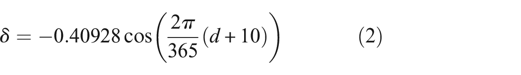
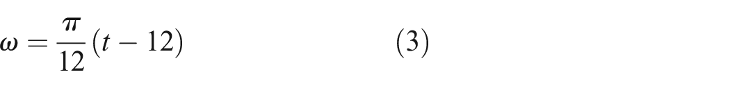
where δ is the sun declination angle; d is the dth day of the year; φ is the latitude angle; ω is the solar hour angle; and t is the local solar time in hours.

Figure 1.

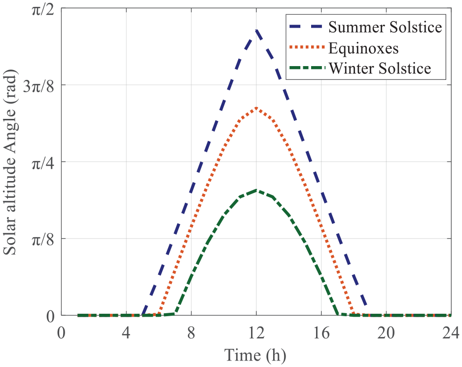
Variation of solar altitude angle throughout the day.

The hours when the weather is clear (i.e., CF is 0–1) from sunrise to sunset are counted and accumulated after multiplying the sin θ of that period as the effective daily sunshine hours, thus improving the accuracy of modeling and predicting the STD. Calculate the duration of sunny weather from sunrise to sunset (i.e., CF is 0–1), multiply it by sin θ of this period, and accumulate it as the effective daily SD, which can improve the accuracy of STD modeling and prediction. The effective SD can be obtained from Equation (4).

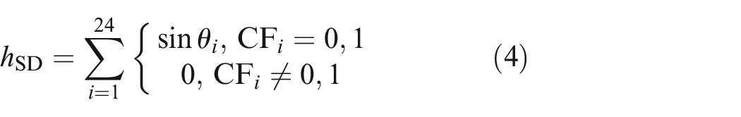
h_{SD} = \sum_{i = 1}^{24} {\begin{matrix} \sin θ_{i}, C F_{i} = 0, 1 \\ 0, C F_{i} \neq 0, 1 \end{matrix}

(4)

Figure 2 shows the specific flow chart of the method. The meteorological data are all obtained from the meteorological center website, where the directly obtained parameters are AT, air pressure (AP), air humidity (AH), WS, CF, and SR; the parameters obtained by computational derivation are daily maximum temperature (T_dmax), daily minimum temperature (T_dmin), daily maximum temperature difference (ATD_d), maximum temperature difference from the previous day (ATD_p), the occurrence of rains (Rain), and effective SD, where the data accuracy is 1 h. Table 1 summarizes the comparison between the meteorological parameters used in previous studies and those used in this study. To consider the influence of complex environmental factors on the STG more comprehensively and to increase the accuracy of relevant modeling, this article considers various influencing factors compared with previous studies and increases five meteorological parameters that have a larger influence on the prediction effect of the STG. The relationship between meteorological parameters and STG can be modeled by using 12 meteorological parameters as input and STG (i.e., multiple consecutive STDs) as output, which enables the estimation of STG by meteorological data.

Figure 2.

Specific flow chart of the proposed methodology.

Table 1.

Meteorological parameter selection.

Meteorological parameters	Previous studies	This study	References
AT	✓	✓	Wang et al.²⁸
WS	✓	✓	Abid et al.²³; Lee and Kalkan²⁴; Liu et al.²⁵; Wang et al.²⁸
WD	✓	—	Wang et al.²⁸
SR	✓	✓	Abid et al.²³; Lee and Kalkan²⁴; Liu et al.²⁵; Wang et al.²⁸; Roberts-Wollman et al.²⁶
T _dmax	✓	✓	Roberts-Wollman et al.²⁶; Lee and Kalkan²⁴
T _dmin	✓	✓	Lee and Kalkan²⁴
T _3-ave	✓	—	Roberts-Wollman et al.²⁶
ATD_d	—	✓	Abid et al.²³; Liu et al.²⁵
ATD_p	—	✓	—
AH	—	✓	Wang et al.²⁸
SD	—	✓	—
Rain	—	✓	—
AP	—	✓	—
CF	—	✓	—

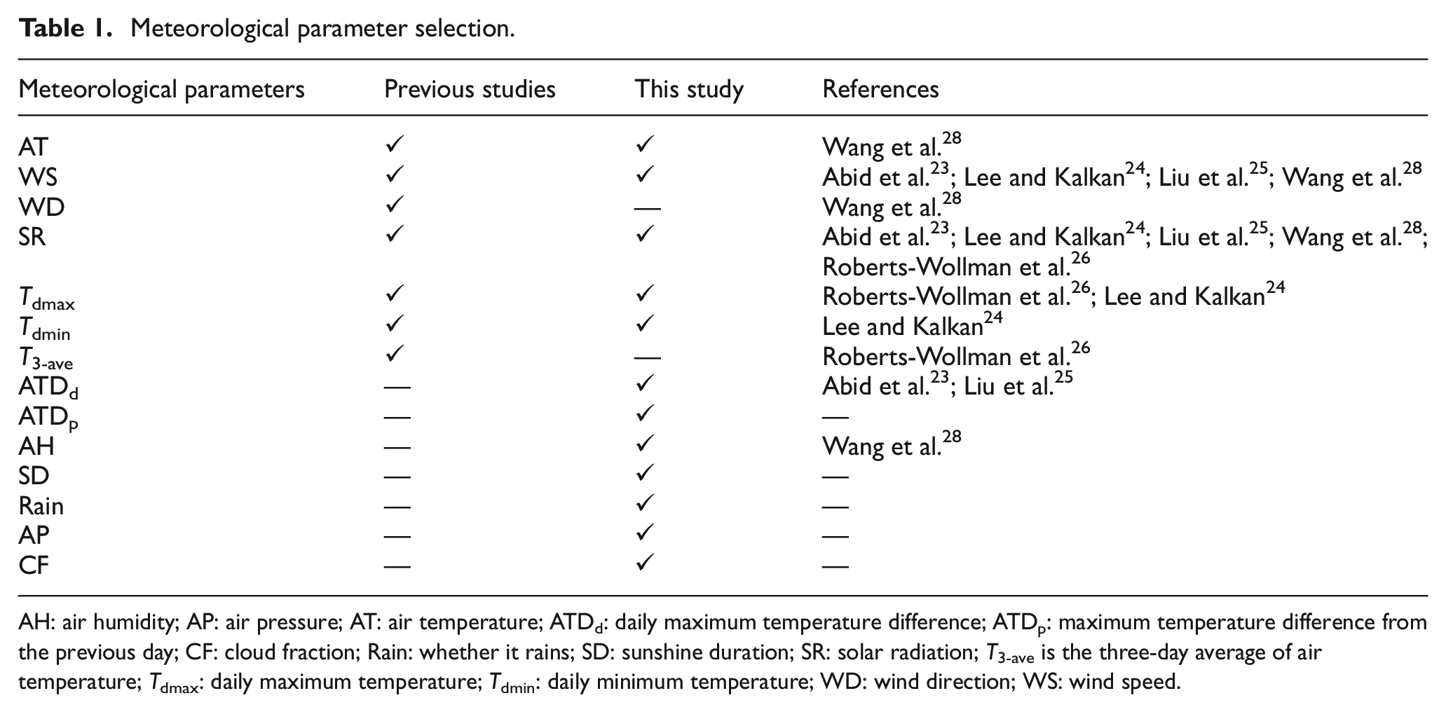
AH: air humidity; AP: air pressure; AT: air temperature; ATD_d: daily maximum temperature difference; ATD_p: maximum temperature difference from the previous day; CF: cloud fraction; Rain: whether it rains; SD: sunshine duration; SR: solar radiation; T_3-ave is the three-day average of air temperature; T_dmax: daily maximum temperature; T_dmin: daily minimum temperature; WD: wind direction; WS: wind speed.

Correlation modeling of STG and meteorological parameters

The training and testing samples should be determined first to ensure that all meteorological conditions can be trained effectively, and on this basis, a reasonable correlation model between the STG and meteorological parameters can be established.

Localized division of training and testing STG dataset

The term STG refers to a continuous STD along a specific direction of the measured section. When multiple monitoring points are used, the difference between adjacent monitoring points forms a temperature gradient vector, the STD is given by Equation (5).

ST D_{ij} = T_{i} - T_{j}

(5)

where STD_ij is the temperature difference between monitoring points i and j; T_i and T_j are the temperatures at measuring points i and j, respectively.

Neural network is used to establish the correlation model between STG and meteorological parameters. To train and validate the neural network model, the STG and meteorological parameter dataset needs to be divided into training set and test set. Due to the different mapping relationships between input and output under different meteorological conditions (such as different seasons, sunny, and rainy conditions), the correlation between meteorological parameters and STG is different²⁸; therefore, it is necessary to make the training process cover all the meteorological situations. However, the structural temperature data currently monitored by the SHM system are only 1–2 years or less, dividing the training sets and test sets chronologically or randomly may result in some data for different meteorological conditions not being effectively trained. When used to predict the STD, the results may not reach the actual STD extremes, which will lead to large errors when used for extremum analysis. Therefore, to establish a regression model that is adequately trained for all meteorological situations, the concept of localized modeling is used to classify the entire data sample by clustering, and then the training and test sets are randomly selected in each part.

The differences in meteorological conditions are mainly reflected in different seasons, different weather conditions such as cloudy, sunny, and rainy, and various diurnal temperature differences; all these different meteorological conditions will have an impact on STG. And these meteorological conditions can be expressed in terms of T_dmax, T_dmin, ATD_d, daily total SR, and the occurrence of rains. Therefore, the five parameters including T_dmax, T_dmin, ATD_d, daily total SR, and the occurrence of rains are selected as clustering indices. The specific process of dividing the dataset is shown in Figure 3. The two-step clustering (TSC) method is introduced for dataset division.

Figure 3.

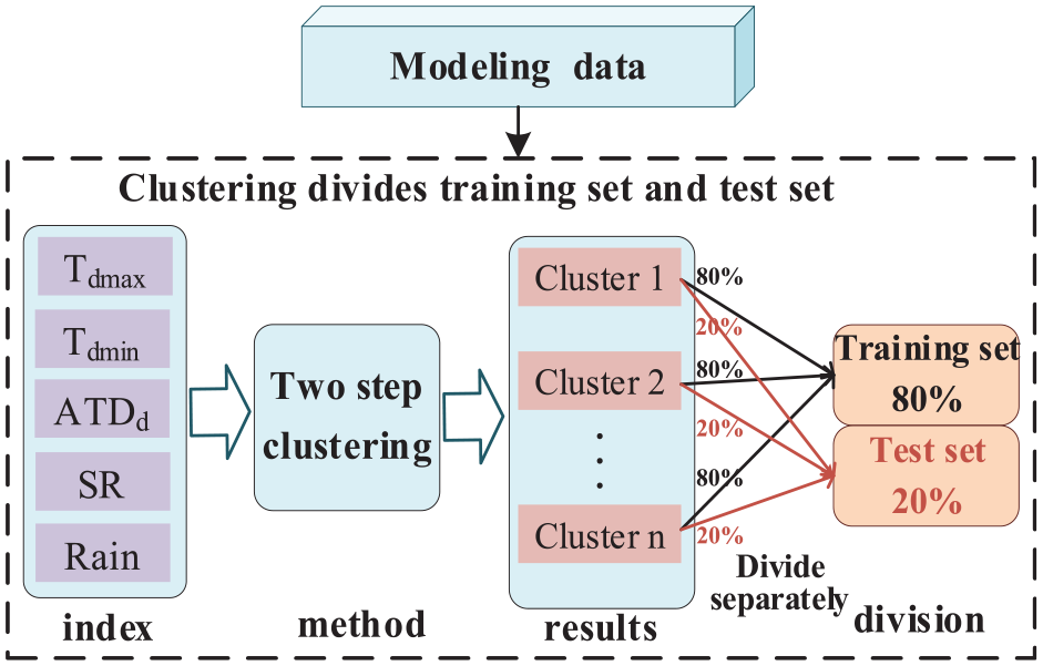
The specific process of dividing the dataset.

The TSC method is an improved method based on balanced iterative reducing and clustering using hierarchies (BIRCH),^31,32 which has the advantage of handling both continuous and categorical meteorological parameters and automatically determining the optimum number of clusters for meteorological conditions. The meteorological parameter sample set can be defined as $X = {x_{1}, x_{2}, \dots, x_{N}}$ containing N days of meteorological features, and each day has n₁ continuous meteorological parameters and n₂ categorical meteorological parameters. The log-likelihood function is used in the TSC to derive the distance measure, and the distance between clusters C_i and C_j is defined by Equations (6) and (7).

d (C_{i}, C_{j}) = ξ_{i} + ξ_{j} - ξ_{{i, j}}

(6)

ξ_{v} = N_{v} (\sum_{k = 1}^{n_{1}} \frac{1}{2} \log ({\hat{σ}}_{k}^{2} + {\hat{σ}}_{vk}^{2}) - \sum_{k = 1}^{n_{2}} \sum_{l = 1}^{L} \frac{N_{vkl}}{N_{v}} \log \frac{N_{vkl}}{N_{v}})

(7)

where $ξ$ is the clustering parameter; $v = i, j$ ; ${i, j}$ represents combining clusters C_i and C_j; N_v is the number of data points in cluster C_v; ${\hat{σ}}_{k}^{2}$ is the estimated variance of the kth continuous meteorological parameter for all records; ${\hat{σ}}_{vk}^{2}$ is the estimated variance of the kth continuous meteorological parameter for records in the vth cluster; L is the number of categories for the kth symbolic meteorological parameter (i.e., classification parameter, which in this article refers to be rainy or not); and N_vkl is the number of records in cluster v, which belongs to the lth category of the kth symbolic meteorological parameter.

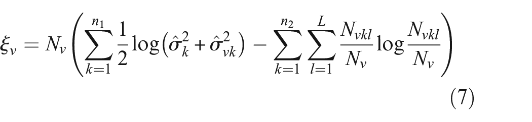
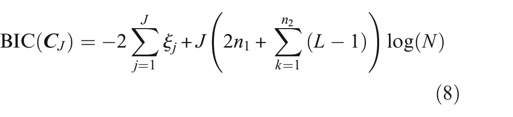
The TSC uses a two-step procedure to automatically determine the number of meteorological condition clusters. The first step is to preliminarily estimate the number of clusters in the meteorological conditions based on the Bayesian information criterion (BIC). The preliminary cluster number is determined when the decrease in BIC diminishes dramatically as the number of clusters increases. The BIC of cluster $C_{J} = {C_{1}, \dots, C_{J}}$ was calculated using Equation (8).

BIC (C_{J}) = - 2 \sum_{j = 1}^{J} ξ_{j} + J (2 n_{1} + \sum_{k = 1}^{n_{2}} (L - 1)) \log (N)

(8)

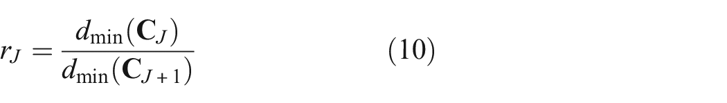
In the second step, the minimum distance for each merge is calculated, as shown in Equation (9). Then, the ratio of the minimum distances of the adjacent merges is used as an index to determine the final cluster number, as denoted by Equation (10). If $r_{S} = max {r_{J} : J \geq 2}$ is obtained, the corresponding cluster number S can be determined as the optimal number. The rationale behind the second step is that the maximum ratio usually occurs when the last two meteorological condition clusters are merged.

d_{min} (C_{J}) = min {d (C_{i}, C_{j}) : i \neq j}

(9)

r_{J} = \frac{d_{min} (C_{J})}{d_{min} (C_{J + 1})}

(10)

The localized subsets based on clustering were divided into 80% and 20% to form the training and test sets,³³ respectively, for modeling the correlation between meteorological parameters and STG.

Correlation modeling

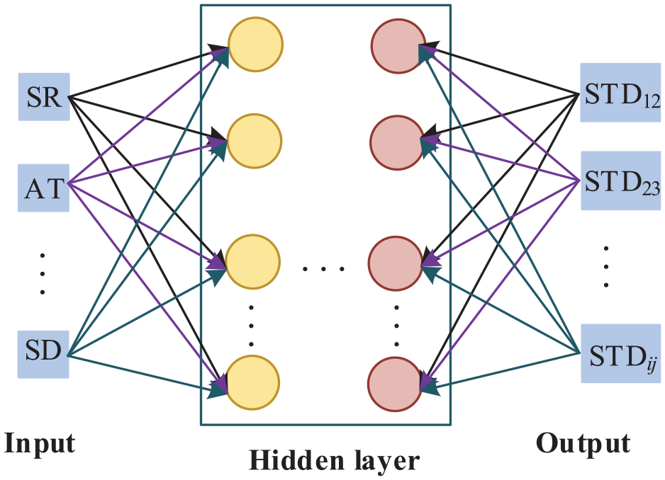
STG can be induced by numerous meteorological parameters, and the influence mechanisms are complex and mostly nonlinear. The back propagation neural network (BPNN) was chosen to construct the meteorological parameter and STG models due to its advantage of being able to approximate any nonlinear mapping relationship with enough hidden layers and nodes and its good generalization capability in complex models.³⁴ The BPNN is a multilayer feedforward network trained by an error backpropagation algorithm. The neural network topology diagram for modeling the relationship between meteorological parameters and temperature gradient is shown in Figure 4, which is composed of a variety of meteorological parameters as an input layer, one or more hidden layers, and multiple STDs as an output layer; each layer contains several artificial neurons.

Figure 4.

Back propagation neural network model topology structure diagram.

The essence of training a network is to adjust the weights and biases given to the network. The training process consists of transmitting output values layer by layer through forward propagation and back-adjusting weights and bias values through backward feedback. The network training process based on the relationship between meteorological parameters and the temperature gradient is shown in Figure 5. According to Zhang et al.,³⁵ the most appropriate BPNN parameters are determined after several trials are performed using the same network structure. Based on literature³⁶ and several trials, the BPNN parameters selected in this article are as follows: The learning rate is 0.01; the activation function of the hidden and output layers are tansig and purelin functions, respectively; the goal error of training is set to 0.001. If the BPNN model cannot reach the training termination, it is enforced to stop after a maximum epoch of 1000.

Figure 5.

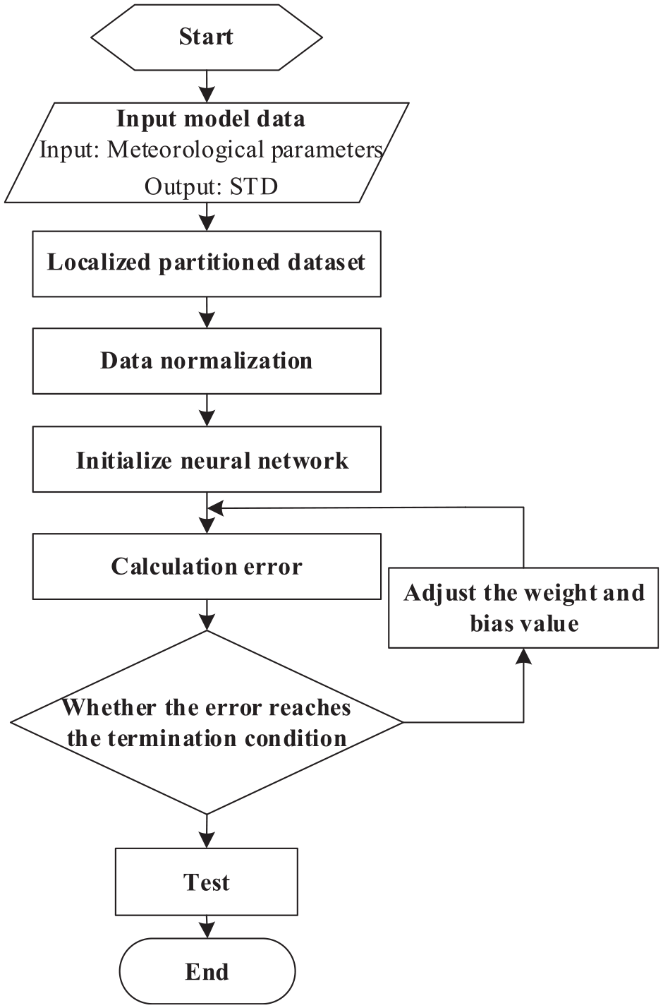
Back propagation neural network training flowchart.

Extension of STG monitoring dataset

The long-term historical meteorological data of a bridge site, including AT, AP, AH, WS, CF, Rain, and SR, can be obtained from the meteorological website, and then meteorological parameters, such as T_dmax, T_dmin, ATD_d, ATD_p, and SD, can be calculated. Modeling the correlation between meteorological parameters and STG using the method presented in section “Correlation modeling of STG and meteorological parameters” enables the effective extension of long-term STG data, which can subsequently be used to calculate representative values of STG for a given return period of the bridge structure.

STG representative value determination

Extreme value analysis of STG

Extreme value analysis is one of the most successful methods for determining representative values of temperature effects for expected return periods, which can characterize the tail behavior of independent continuous random variables based on the statistical properties of the extreme values of maximum values in a dataset.^37,38 The main methods of extreme value analysis commonly used in current research include the block maxima (BM) method and the POT method.

The BM method is a technique for modeling the generalized extreme value (GEV) distribution. This method generally divides STD data samples into equal-sized and nonoverlapping blocks and then extracts the maximum value of each block. The GEV distribution is a unified expression of the Gumbel distribution, Frechet distribution, and Weibull distribution, and the cumulative distribution function of the GEV distribution is shown in Equation (11).

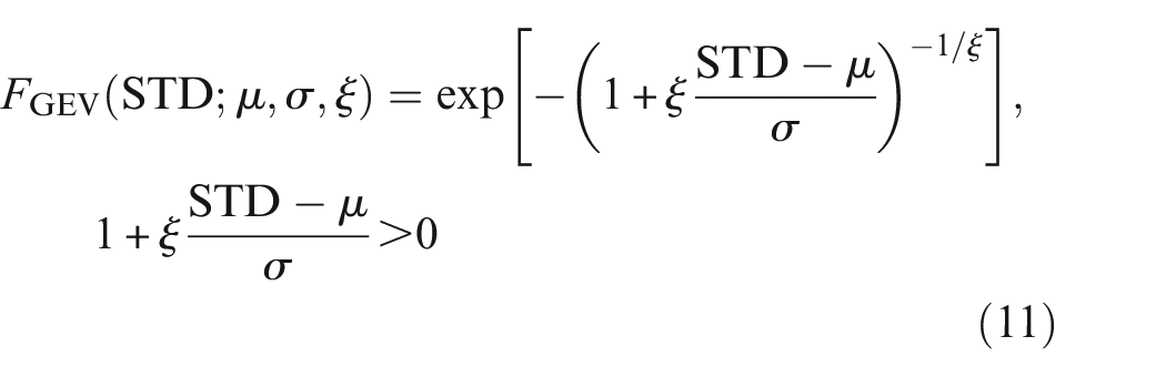
\begin{matrix} F_{GEV} (STD; μ, σ, ξ) = \exp [- {(1 + ξ \frac{STD - μ}{σ})}^{- 1 / ξ}], \\ 1 + ξ \frac{STD - μ}{σ} > 0 \end{matrix}

(11)

where μ is the location parameter; σ is the scale parameter; and ξ is the shape parameter.

However, due to the insufficient monitoring duration of the bridge SHM system, the BM method used for temperature gradient analysis mainly uses daily extremes, which results in many low extremes in the samples used for extreme value analysis and may lead to unreasonable estimation results of temperature gradient representatives. Distinct from the BM method, the POT method selects the STD data that exceeds the threshold value u as the sample, where the objects are the excess values random variables. When the threshold is set large enough, the excess distribution necessarily converges to the generalized Pareto (GP) distribution, which emphasizes the statistical characteristics of the samples in the tail region. The mean exceed function for the POT method was used to determine the threshold,³⁹ and the cumulative distribution function of GP distribution is shown in Equation (12).

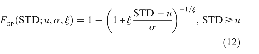
F_{GP} (STD; u, σ, ξ) = 1 - {(1 + ξ \frac{STD - u}{σ})}^{- 1 / ξ}, STD \geq u

(12)

where μ is the threshold; σ is the scale parameter; and ξ is the shape parameter.

STG representative value determination based on extreme value analysis

The probability p for STD exceeding the extreme value for the R-year return period of thermal action assumed can be calculated using Equation (13).

p = \frac{1}{R \times n}

(13)

where R is the return period and n is the number of STD data in a full year.

The maximum possible temperature gradient value of the bridge structure during a certain time is the representative value of the temperature gradient in a given return period. The representative values of the bridge temperature gradient return period described by the GEV and GP distributions are calculated as shown in Equations (14) and (15), respectively.

p = 1 - F_{GEV} (STD; μ, σ, ξ) = \int_{ST D_{e}}^{+ \infty} f_{GEV} (STD; μ, σ, ξ) d STD

(14)

p = 1 - F_{GP} (STD; u, σ, ξ) = \int_{ST D_{p}}^{+ \infty} f_{GP} (STD; u, σ, ξ) d STD

(15)

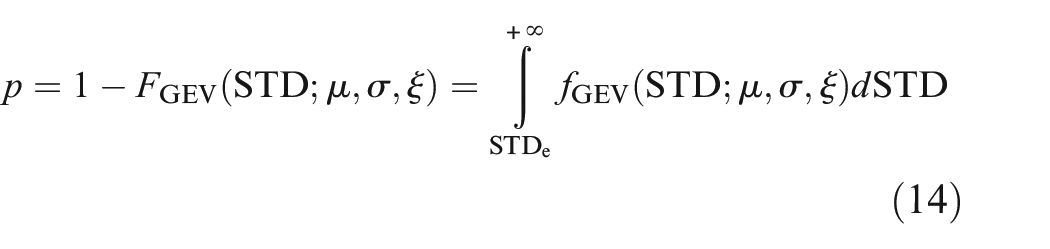
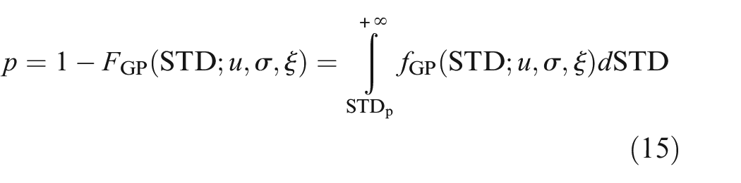
where STD_e and STD_p are representative values of the STD for a given return period of the bridge calculated by the GEV and GP distributions, respectively.

Case study

Bridge description

Using a cable-stayed bridge as an example, the proposed method for the determination of STG representative values based on meteorological data is verified. The bridge is located is located in the northern hemisphere (121.73° east longitude and 29.96° north latitude). It is an asymmetric single-tower cable-stayed bridge with a multi-cell box concrete girder and the main span of 567 m. The dimensions and sections C, N and D temperature sensor layout are shown in Figure 6. The data sample was from October 1, 2015 to November 31, 2016, with 322 days of valid structural temperature data after the removal of breakpoints, containing four seasonal variation characteristics, where temperature sensors were sampled at a frequency of 1 h.

Figure 6.

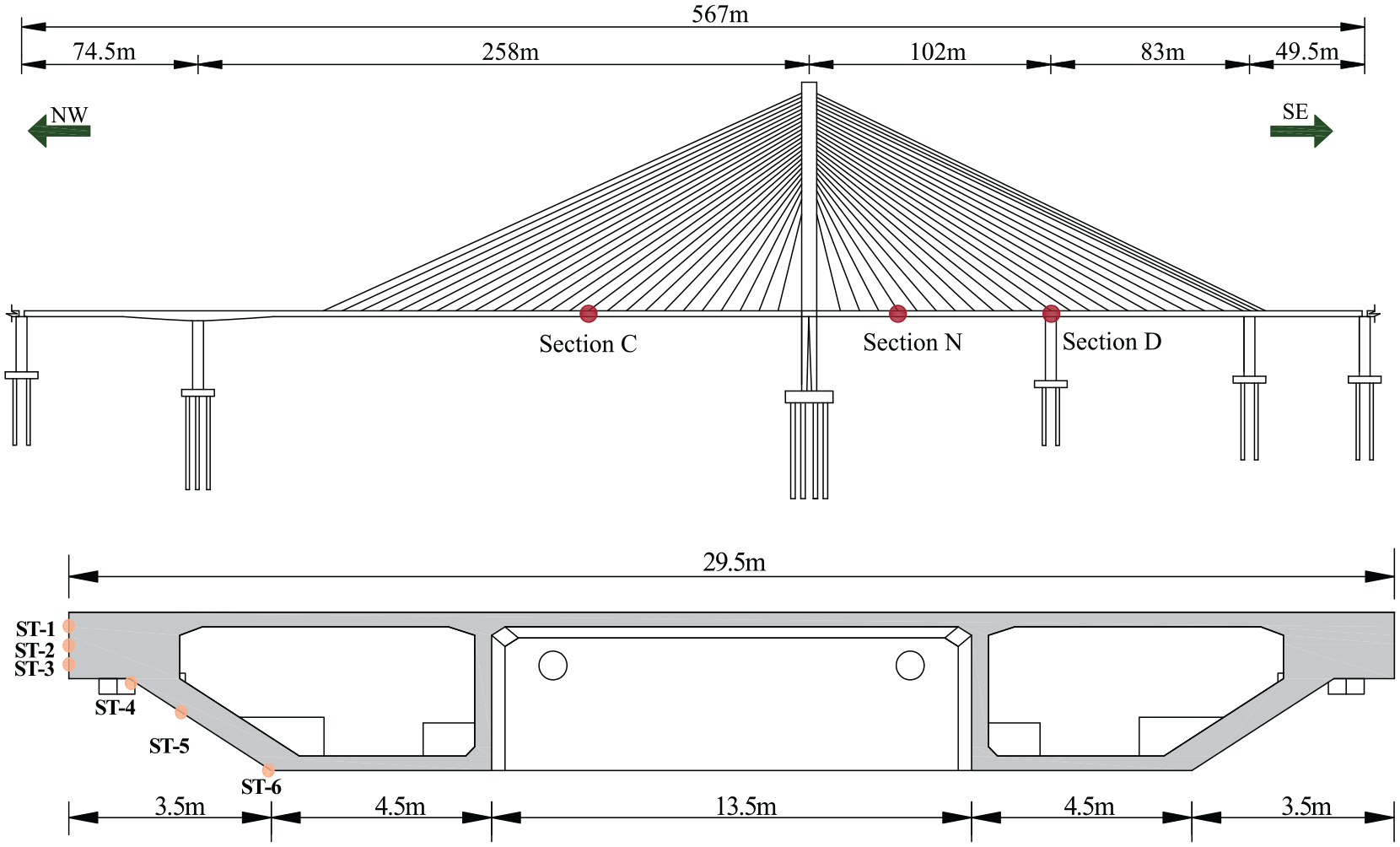
Configurations of prototype bridge: (a) elevation view and (b) section layout of temperature sensor.

Correlation analysis between STD and meteorological parameters

Figure 7 shows the bridge structure temperature variation. Figure 7(a) and (b) show that the temperature variation trends, and magnitude range are relatively the same for sections C, N and D, which indicates that the vertical temperature variation in different sections is small along the longitudinal bridge direction (as shown in Figure 7(d)). Therefore, section C is selected as an example for vertical temperature gradient analysis. In addition, Figure 7(c) shows the correlation of structural temperature of section C with meteorological temperature and weather conditions (i.e., cloudy, sunny, and rainy) in February 2016, which markedly indicates that structure temperature is positively correlated with meteorological temperature and is more likely to have a larger STD on sunny days than on cloudy days. In contrast, the situation is different on rainy days and requires further analysis.

Figure 7.

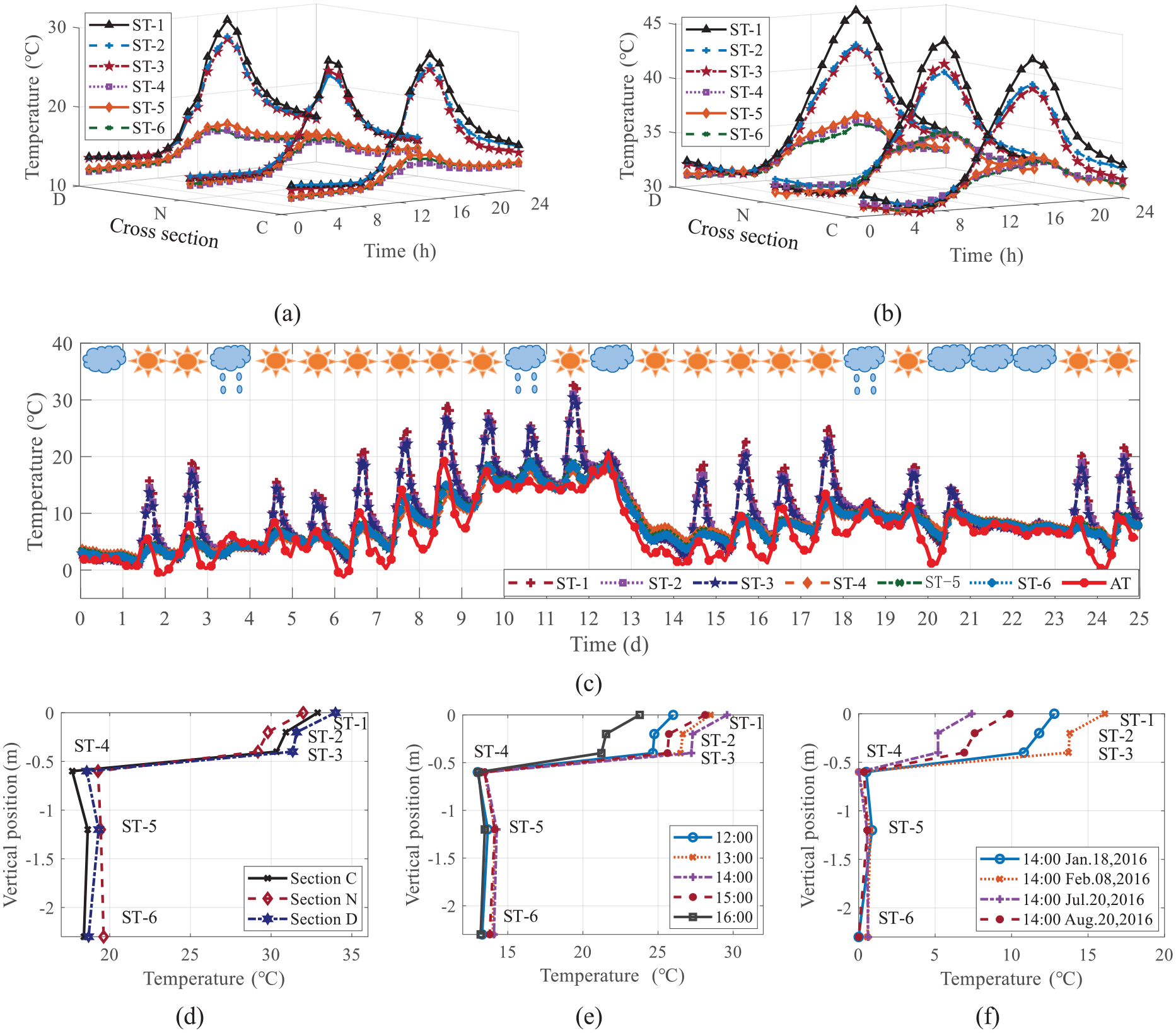
Bridge structural temperature variation: (a) structural temperature along longitudinal bridge direction in January, (b) structural temperature along longitudinal bridge direction in August, (c) structural and meteorological temperature variations in February, (d) vertical temperature variation of different sections at the same time, (e) vertical temperature variation of section C at different times on February 8, 2016, and (f) vertical STG variation of section C in different months.

Figure 7(e) illustrates the vertical temperature variation at different moments on February 8, 2016, with the maximum temperature gradient occurring at approximately 14:00. The largest STD between ST-3 and ST-4 is because SR strikes the horizontal surface at an angle from a high altitude, with the SR affecting the top plate more than the web and bottom plate, while ST-4 is located at the junction of the top plate and the diagonal web and receives the least SR. As a result, the temperature of the top slab increases significantly during the day compared to the web and bottom slab and then transfers to the web and bottom slab slowly, resulting in a large vertical temperature gradient. Figure 7(f) shows the vertical STG variation for different months which is calculated taking the vertical minimum temperature as a reference. It is observed that the vertical STG in winter is larger than that in summer because the bridge structure is subjected to higher environmental temperature in summer than in winter, resulting in a lower STD between the top plate and the web than in winter.

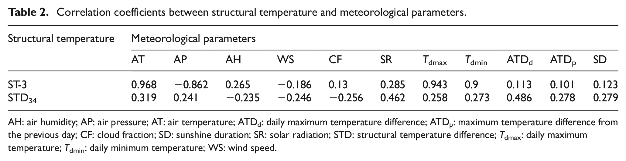
The STD₃₄ (STD between ST-3 and ST-4) and ST-3 were used as an illustration to analyze the correlation between STD and structural temperature and meteorological parameters, and the correlation coefficient matrix is shown in Table 2. From Table 2, the following characteristics can be found: (i) The structural temperature has the strongest correlation with the meteorological temperature, but the correlation between the STD and the meteorological temperature is significantly reduced; (ii) The STD is correlated with all the obtained meteorological parameters, but it is not a simple linear relationship, for which it is necessary to apply nonlinear methods to establish their correlation models.

Table 2.

Correlation coefficients between structural temperature and meteorological parameters.

Structural temperature	Meteorological parameters
Structural temperature	AT	AP	AH	WS	CF	SR	T _dmax	T _dmin	ATD_d	ATD_p	SD
ST-3	0.968	−0.862	0.265	−0.186	0.13	0.285	0.943	0.9	0.113	0.101	0.123
STD₃₄	0.319	0.241	−0.235	−0.246	−0.256	0.462	0.258	0.273	0.486	0.278	0.279

AH: air humidity; AP: air pressure; AT: air temperature; ATD_d: daily maximum temperature difference; ATD_p: maximum temperature difference from the previous day; CF: cloud fraction; SD: sunshine duration; SR: solar radiation; STD: structural temperature difference; T_dmax: daily maximum temperature; T_dmin: daily minimum temperature; WS: wind speed.

Establishing correlation models

It is necessary to divide the sample data into a training set and a test set before using a BPNN to establish the correlation model. Because the current bridge health monitoring system only has recorded approximately 1 year of structural temperature data, to ensure that all meteorological conditions in a year can be effectively trained, a localized sample subset is constructed using the localized division method proposed. T_dmax, T_dmin, ATD_d, daily total SR, and rain are selected as clustering indices. Based on these parameters, the data samples were classified into three different weather conditions using a TSC method, and the clustering results are shown in Figure 8 as rainy weather, low temperature weather, and high temperature weather. Eighty percent of each weather condition is selected as the training set, and 20% is selected as the test set. Taking STD₃₄ as an example, the training and test results are shown in Figure 9. It can be observed that the training and test sets are well fitted at the extreme values of temperature difference and can satisfy the accuracy requirement of temperature gradient analysis. To verify the effectiveness of the proposed method, the training and prediction correlation coefficients and root mean square error (RMSE) of the following four regression models are compared in Table 3.

Model 1: BPNN, divides the dataset by clustering using the 12 meteorological parameters analyzed.

Model 2: BPNN, randomly divides the dataset using the 12 meteorological parameters analyzed.

Model 3: BPNN, divides the dataset by clustering using the seven meteorological parameters (AT, AH, WS, SR, T_dmax, T_dmin, and ATD_d) proposed in the previous study.

Model 4: Linear regression, using the 12 meteorological parameters analyzed.

Figure 8.

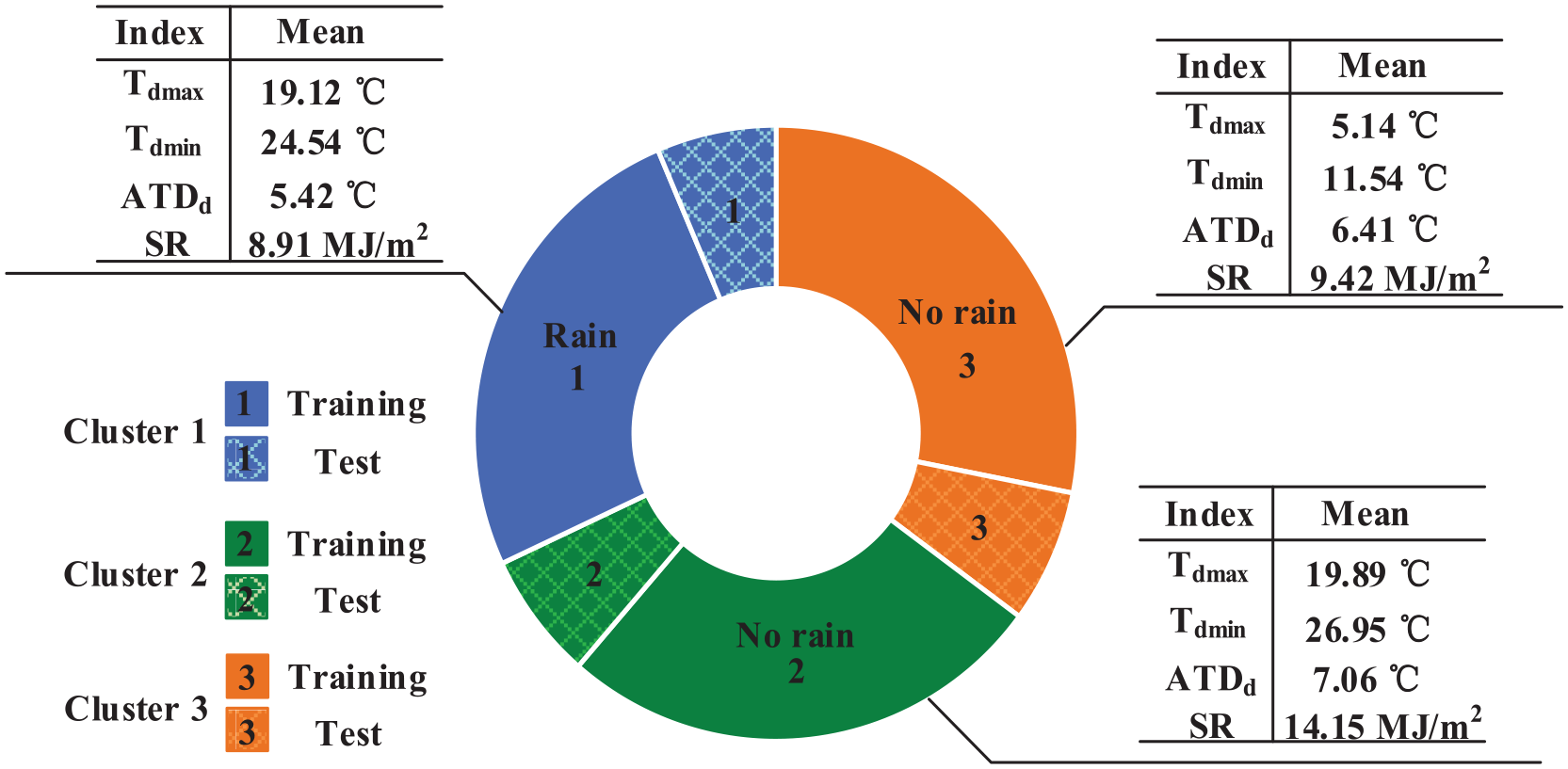
Localized sample subset clustering and dataset division results.

Figure 9.

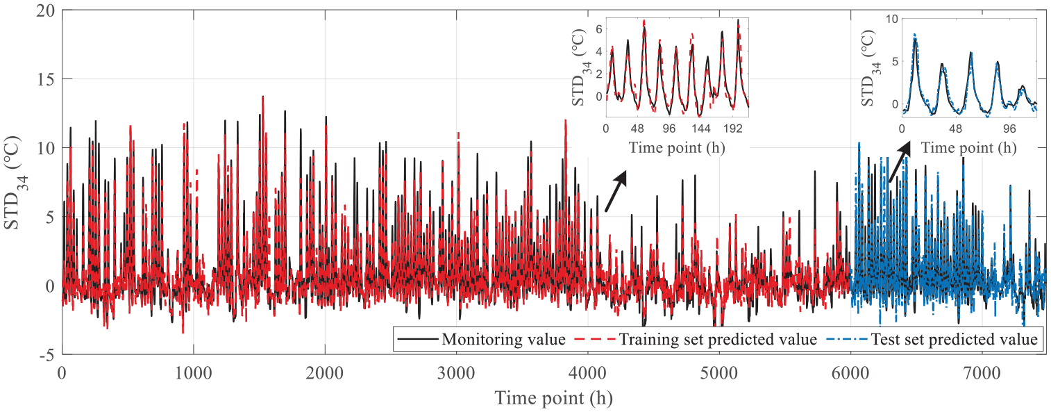
Training and test results.

Table 3.

Comparison of the results of the four regression models.

Index	Model 1		Model 2		Model 3		Model 4
Index	Training	Test	Training	Test	Training	Test	Training	Test
R	0.92	0.89	0.85	0.81	0.83	0.79	0.73	0.71
RMSE	0.94	0.96	1.33	1.42	1.30	1.36	1.49	1.56

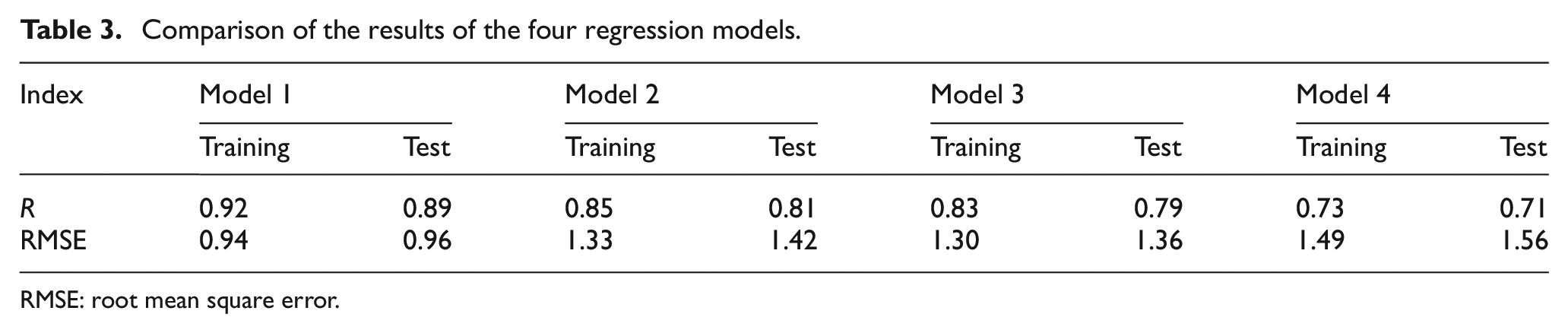
RMSE: root mean square error.

The following conclusions can be drawn from the results: (i) A stronger correlation can be obtained through the training and testing dataset constructed by the proposed localized clustering method than the randomly divided dataset, in which more meteorological parameters of the dataset were analyzed and considered than in past studies; (ii) The simple linear regression used to describe the relationship between STD and meteorological parameters not only has poor correlation and large error but also does not fit well for the extreme values of the STD. Therefore, simple linear regression is not sufficient to describe the relationship between meteorological parameters and STD, while the proposed method has good training and generalization ability.

Regression models are obtained by four advanced algorithms,^39,40 radial basis function neural network, generalized regression neural network, support vector regression, and random forest model, and the results are compared with the BPNN model. The dataset division, parameter selection, and training volume of the four models are the same as described in Model 1 of the previous BPNN model to avoid bias in the comparison. The comparison results are shown in Table 4. The results show that the prediction accuracy of STG using BPNN is similar to that of advanced networks and machine learning models, and even has higher accuracy and generalization performance. Moreover, BPNN is a traditional neural network model with high generalization and self-adaptation ability, and simple and convenient usage performance. Therefore, in this article, BPNN is chosen to establish a relevant model to extend the long-term STG dataset.

Table 4.

Comparative results of different regression methods.

Index	BPNN		RBFNN		GRNN		SVR		RF
Index	Training	Test	Training	Test	Training	Test	Training	Test	Training	Test
R	0.92	0.89	0.90	0.89	0.98	0.71	0.93	0.88	0.97	0.88
RMSE	0.94	0.96	0.97	1.06	0.89	1.55	0.86	1.04	0.55	0.96

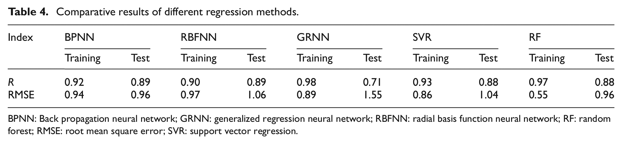
BPNN: Back propagation neural network; GRNN: generalized regression neural network; RBFNN: radial basis function neural network; RF: random forest; RMSE: root mean square error; SVR: support vector regression.

The temperature sensors of the prototype bridge SHM system are deployed on the surface of the bridge structure; these readings do not represent the temperature in the middle of the bridge cross-section. However, since the bridge structure is subject to common environmental action, if enough temperature sensors are placed in the middle of the bridge cross-section, the correlation between meteorological parameters and internal STG can also be well established, without affecting the verification of the method in this article.

Determination of STG representative values based on 10-year meteorological parameters

The amount of 1-year temperature monitoring sample data is too small to derive representative values of temperature action for return periods of more than 50 years. For this reason, the long-term STG samples were estimated further using the constructed correlation model with a total of 10 years of historical meteorological data from 2011 to 2021 recorded by the local meteorological station, and the estimated results are shown in Figure 10 for STD₃₄ as an illustration. The annual trend of the estimated sample and the range of temperature difference magnitudes show that the estimated results are reasonable.

Figure 10.

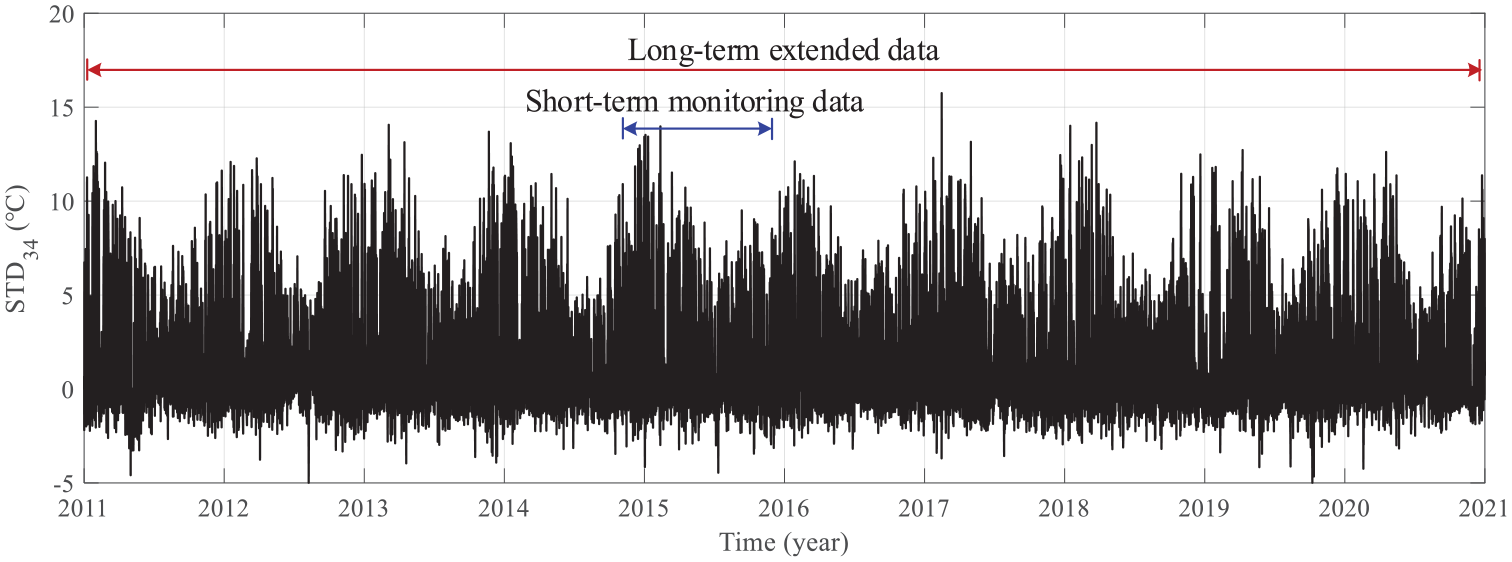
Estimated results of structural temperature difference for 10 years.

To verify the validity of the proposed method for estimating long-term STG data and determining the STG representative values for a given return period, STD₃₄ is used as an example to show the calculation results. To ensure no correlation between the samples taken out, the daily STD extremes for the 10 years of data were selected, and then the samples exceeding the threshold value are furtherly obtained from the daily STD extremes. The mean exceed function is shown in Figure 11(a). The plot has zero slope near 11.1°C, so the threshold value u = 11.1 is set. For the same10-year STG data, the POT method was adopted to select extreme value samples, and the fitting results are shown in Figure 11(b), which shows that the extreme samples fit the GP distribution well. Since there are not enough monitoring data for 1 year, it is difficult to ensure that the samples exceeding the threshold are not taken from the same day, which means that the independence of the extreme samples of STG cannot be guaranteed. Therefore, the analysis using the POT method for 1-year data is not discussed here.

Figure 11.

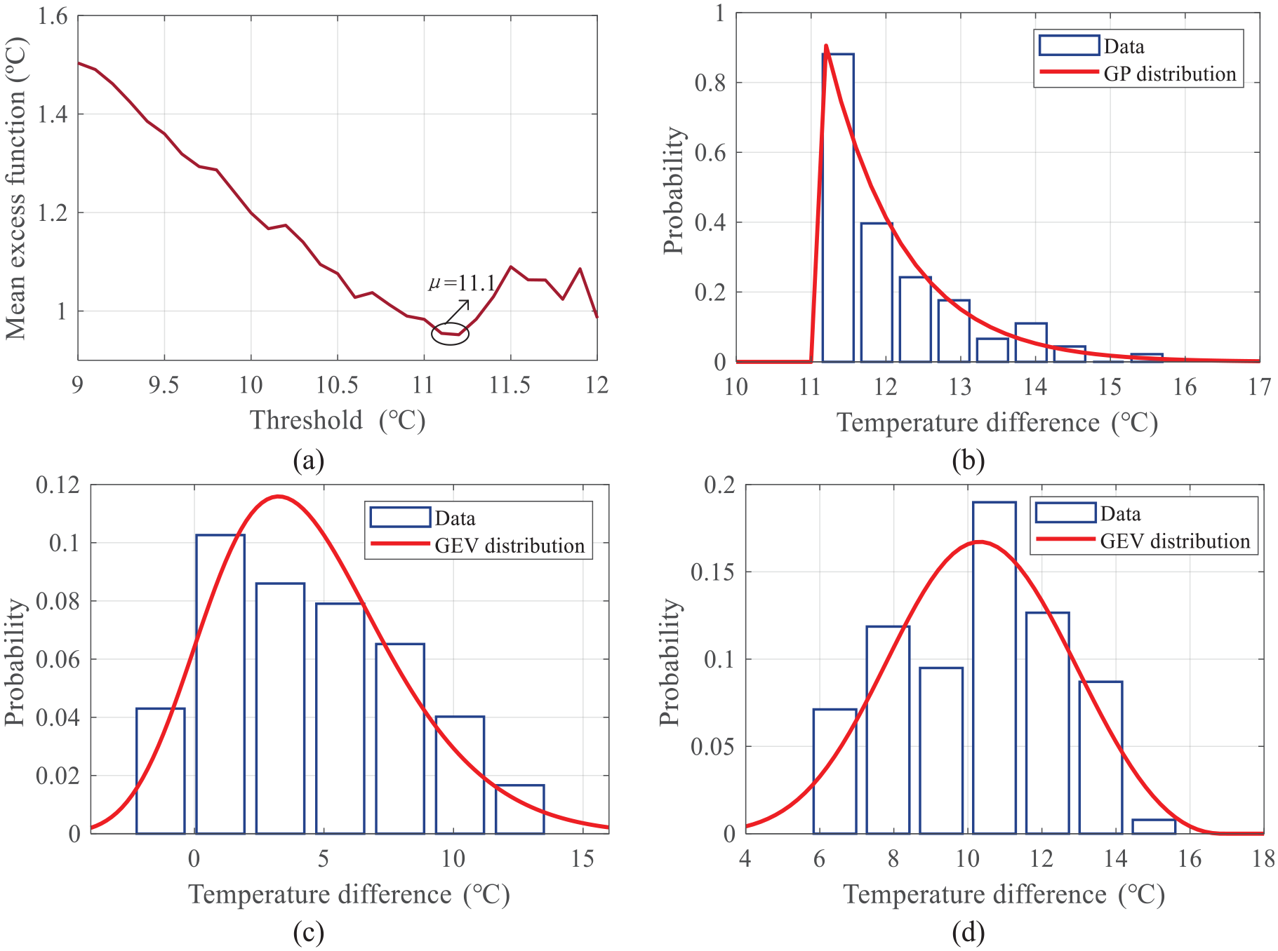
Structural temperature difference extreme value distribution probability distribution: (a) mean residual life plot, (b) 10 years peak over threshold, (c) 1 year block maxima (BM), and (d) 10 years BM.

Figure 11(c) and (d) show the results of the extreme value analysis using the BM method based on short-term STG monitoring data (1 year) and long-term extended STG data obtained through the proposed method (10 years), respectively. Figure 11(c) is the result obtained by using the current common analysis method, and the BM method used in Figure 11(d) is selected with the same number of extreme value samples as the POT method. The distribution parameters and the representative values of the given return periods are shown in Table 5. The results can be found as follows: (i) The 10-year representative value of STD₃₄ calculated from 1-year monitoring data is 20.9°C, but the actual maximum extreme value of 10 years is only 15.74°C, indicating that using the daily extreme value method for short-term monitoring data may lead to unreasonable results of STD representative values; (ii) The STD representative value of the 100-year return period calculated from the 10-year data is slightly larger than the extreme value of the actual estimated temperature difference in 10 years and is in a reasonable range, which proves the rationality of the results; (iii) The BM method may lead to some extreme values not being selected in the final extreme value sample, but the sample data in the period of low extreme values are selected.⁴¹ In contrast, the data selected using the POT method are large extreme value samples during this year, which can make more effective use of the data and make the calculation results more reasonable.

Table 5.

Calculation results of representative values for different dataset of structural temperature.

Data type	Distribution	ξ	µ(°C)	σ(°C)	Sample extreme (°C)	Representative values (°C)
Data type	Distribution	ξ	µ(°C)	σ(°C)	Sample extreme (°C)	10 years	50 years	100 years
1 year BM	GEV	−0.09	2.76	3.16	14.71	20.90	22.86	23.71
10 years BM	GEV	−0.33	2.36	9.49	15.74	—	15.75	15.95
10 years POT	GP	−0.03	11.10	1.00	15.74	—	16.61	17.16

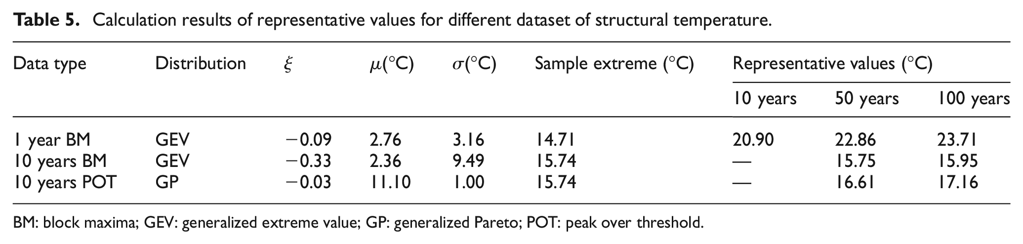
BM: block maxima; GEV: generalized extreme value; GP: generalized Pareto; POT: peak over threshold.

In this study, the POT method was used to calculate the representative values of STD₁₂, STD₂₃, STD₄₅, and STD₅₆ and obtain the temperature gradient model for the case structure, with the results shown in Figure 12 and Table 6. According to Figure 12 and Table 6, the following conclusions can be found: (i) The upper part of the calculated temperature gradient model is close to that of the bifold model, which is like the temperature gradient model given by the AASHTO zone 2⁶ and the Chinese highway code,⁷ and the lower part has a negative temperature gradient like that of the AASHTO code. However, the first kink given by the code is generally 100 mm deep from the top edge of the beam section, and the second kink is generally 400 mm deep. Compared with the model, the slope of the code is higher, and the temperature gradient decreases too fast; (ii) The maximum temperature gradient of the bridge surface given by the Chinese highway code is 20°C, while the counterpart from the proposed method is 23°C. Therefore, it may be difficult for the code to envelop the long-term calculation results of the temperature gradient of the concrete box girder structure here.

Figure 12.

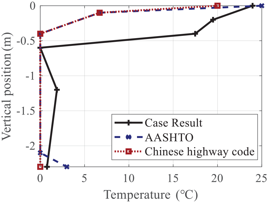
Comparison of vertical structural temperature gradient.

Table 6.

Representative values of structural temperature gradient for given return period.

Temperature gradient	GP distribution parameter			Representative values (°C)
Temperature gradient	ξ	µ(°C)	σ(°C)	50 years	100 years
STD₁₂	−0.13	3.20	0.29	4.37	4.46
STD₂₃	−0.18	1.1	0.23	1.97	2.02
STD₃₄	−0.03	11.10	1.00	16.61	17.16
STD₄₅	−0.17	−0.27	0.32	−1.84	−1.88
STD₅₆	−0.16	0.71	0.10	1.10	1.12

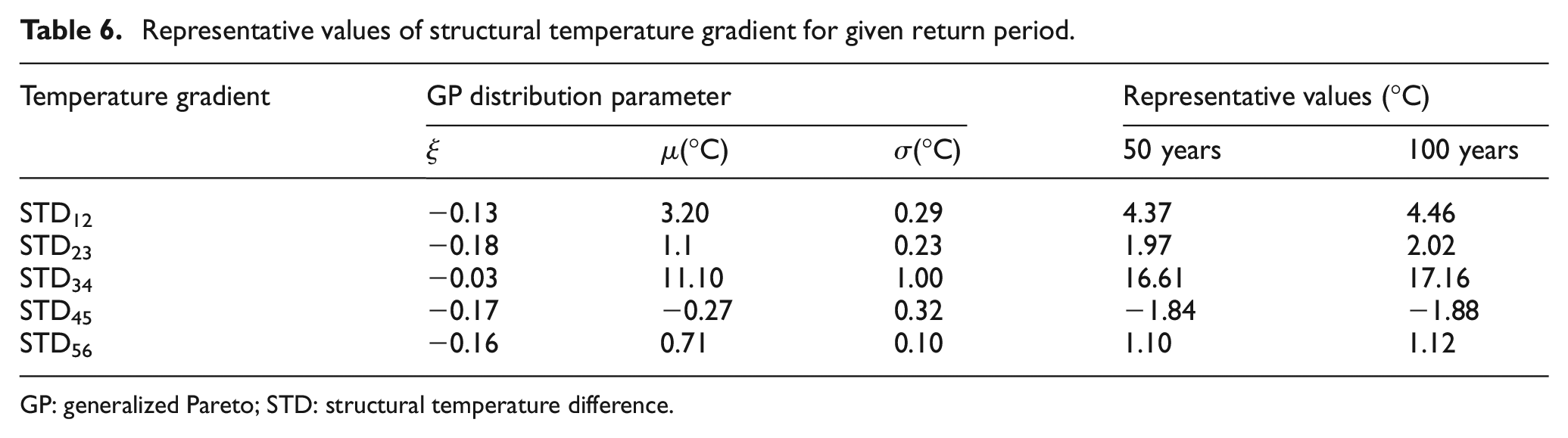
GP: generalized Pareto; STD: structural temperature difference.

Conclusions

This study proposes a method for predicting STG based on meteorological parameters at bridge sites. By considering the coupling action of a variety of meteorological factors, the correlation model between meteorological parameters and short-term STG monitoring data is established. On this basis, the long-term bridge STG is estimated, and more reasonable STD representative values can be determined. Finally, using a large-span cable-stayed bridge as an example, the feasibility and reasonableness of the method are verified. Based on the analysis results, the following conclusions can be drawn:

The correlation analysis between meteorological parameters and structural temperature and STD shows that structural temperature and STD have a strong correlation with AT, AP, and SR and a weak correlation with CF, WS, and AH; also, CF, SD, WS, and SR have a much stronger correlation with STD than structural temperature. The correlation and error analysis verified that the correlation model obtained by the 12 meteorological parameters proposed here is more reasonable than that in previous studies, and the effect of complex meteorological environments on the STG can be more adequately considered.

The proposed method of localized division of STG training and testing sets can consider different meteorological conditions and ensure that all meteorological situations during the monitoring time can be trained effectively. Compared with the method of randomly dividing datasets, the training and testing quality are significantly improved, which proves the effectiveness of the proposed method. In addition, neural network modeling can achieve more accurate prediction results than linear regression methods, which can better describe the relationship between meteorological parameters and STG.

Based on the correlation model between monitored structural temperature and long-term historical meteorological data at bridge sites, the long-term STG of bridges can be estimated, and the STG monitoring dataset can be effectively extended. On this basis, the POT method can be effectively used to obtain more samples of extreme temperature than the BM method. Compared with the short-term temperature monitoring data, the extended long-term temperature dataset can yield an STG representative value much closer to the actual extreme values, which is more reasonable for analyzing the temperature-induced structural responses.

Compared with the STG model proposed by the Chinese code, the actual STG model obtained through the monitoring data in the case study achieves a larger value of STD at the top side of the bridge girder. This means that the STG can be underestimated by the code in some conditions, which can result in risky analysis of the temperature effects on bridge structures. This method is not limited by the type and location of the bridge, but depends on the structural temperature monitoring data of SHM. Setting the temperature sensor of SHM system on the cross-section of the bridge will give more reasonable results for STG analysis.

Footnotes

Declaration of conflicting interests

The author(s) declared no potential conflicts of interest with respect to the research, authorship, and/or publication of this article.

Funding

The author(s) disclosed receipt of the following financial support for the research, authorship, and/or publication of this article: This research work was jointly supported by the National Natural Science Foundation of China (Grants Nos. 52078102 and 52250011), the Fundamental Research Funds for the Central Universities (Grant No. DUT21JC38), and Key Laboratory of Performance Evolution and Control for Engineering Structures in Tongji University, Ministry of Education (Grant No.2022KF-1).

ORCID iDs

Dong-Hui Yang

Ting-Hua Yi

References

Hagedorn

Marti-Vargas

Dang

, et al. Temperature gradients in bridge concrete I-girders under heat wave. J Bridge Eng 2019; 24(8): 04019077.

Yang

, et al. Correlation-based estimation method for cable-stayed bridge girder deflection variability under thermal action. J Perform Constr Fac 2018; 32(5): 04018070.

Algohi

Svecova

Mufti

, et al. Long-term study on the effect of temperature on composite action and variation of neutral axis in slab on girder bridges. Struct Health Monit 2020; 19(5): 1577–1589.

Zhu

Wang

Mao

, et al. Investigation of temperature effects on steel-truss bridge based on long-term monitoring data: case study. J Bridge Eng 2020; 25(9): 05020007.

British Standards Institution (BSI). Steel, concrete and composite bridges-part2: specification for loads. BS 5400-2. London: BSI, 1978.

AASHTO. AASHTO LRFD bridge design specifications. 8th ed. Washington, DC: AASHTO, 2017.

Guobiao Standard (GB). General specifications for design of high-way bridges and culverts. JTG D60-2015. Beijing: China’s Ministry of Transport, 2015.

Nasr

Kjellström

Björnsson

, et al. Bridges in a changing climate: a study of the potential impacts of climate change on bridges and their possible adaptations. Struct Infrastruct Eng 2019; 16(4): 738–749.

Lawson

Ryan

Buckle

. Bridge temperature profiles revisited: thermal analyses based on recent meteorological data from Nevada. J Bridge Eng 2020; 25(1): 04019111.

10.

Peiretti

Parrotta

Oregui

, et al. Experimental study of thermal actions on a solid slab concrete deck bridge and comparison with Eurocode 1. J Bridge Eng 2014; 19(10): 04014041.

11.

Fan

Liu

. Experiment study and refined modeling of temperature field of steel-concrete composite beam bridges. Eng. Struct 2021; 240: 112350.

12.

Tome

Pimentel

Figueiras

. Structural response of a concrete cable-stayed bridge under thermal loads. Eng Struct 2018; 176:652–672.

13.

Xin

Wang

, et al. Effect of temperature loading on the performance of a prestressed concrete bridge in Oklahoma: probabilistic modelling. Structures 2021; 34: 1429–1442.

14.

Zhang

Liu

, et al. Validation of long-term temperature simulations in a steel-concrete composite girder. Structures 2020; 27: 1962–1976.

15.

Cai

Huang

, et al. Investigation of concrete box girder positive temperature gradient patterns considering different climatic regions. Structures 2022; 35: 591–607.

16.

Elshoura

Okeil

. Calibration of temperature gradient load factor for service limit state design of concrete slab-on-girder bridges. J Bridge Eng 2022; 27(11): 04022112.

17.

Yang

, et al. Cable anomaly detection driven by spatiotemporal correlation dissimilarity measurements of bridge grouped cable forces. Smart Struct Syst 2022; 30(6): 661–671.

18.

Zhang

Liu

Deng

. Temperature gradient modeling of a steel box-girder suspension bridge using Copulas probabilistic method and field monitoring. Adv Struct Eng 2020; 24(5): 136943322097177.

19.

Xia

Zhang

Tian

, et al. Experimental study of thermal effects on a long-span suspension bridge. J Bridge Eng 2017; 22(7): 04017034.

20.

Elshoura

Okeil

. Study of statistical uncertainties for temperature gradients in concrete bridges. ASCE-ASME J Risk Uncertainty Eng Syst, Part A: Civ Eng 2022; 8(1): 04021083.

21.

Zhou

Chen

, et al. A generalized pareto distribution-based extreme value model of thermal gradients in a long-span bridge combining parameter updating. Adv Struct Eng 2016; 20(2): 202–213.

22.

Gottsäter

Larsson Ivanov

. Spatial temperature differences in portal frame bridges. Struct Eng Int 2020; 30(2): 254–261.

23.

Abid

Tayşi

Özakça

. Experimental analysis of temperature gradients in concrete box-girders. Constr Build Mater 2016; 106: 523–532.

24.

Lee

Kalkan

. Analysis of thermal environmental effects on precast, prestressed concrete bridge girders: temperature differentials and thermal deformations. Adv Struct Eng 2012; 15(3): 447–459.

25.

Liu

Zhang

, et al. Prediction formula for temperature gradient of concrete-filled steel tubular member with an arbitrary inclination. J Bridge Eng 2020; 25(10): 04020076.

26.

Roberts-Wollman

Breen

Cawrse

. Measurements of thermal gradients and their effects on segmental concrete bridge. J Bridge Eng 2002; 7(3): 166–174.

27.

Feng

Jinyi

Lei

. Experimental investigation of temperature gradients in a three-cell concrete box-girder. Constr Build Mater 2022; 335: 127413.

28.

Wang

Zhang

, et al. Temperature prediction of flat steel box girders of long-span bridges utilizing in situ environmental parameters and machine learning. J Bridge Eng 2022; 27(3): 04022004.

29.

Lei

Fan

Jiang

, et al. Temperature field boundary conditions and lateral temperature gradient effect on a PC box-girder bridge based on real-time solar radiation and spatial temperature monitoring. Sensors 2020; 20(18): 5261.

30.

Herrería-Alonso

Suárez-González

Rodríguez-Pérez

, et al. A solar altitude angle model for efficient solar energy predictions. Sensors 2020; 20(5): 1391.

31.

Chiu

Fang

Chen

, et al. A robust and scalable clustering algorithm for mixed type attributes in large database environment. In: Provost

Srikant

(eds.) Proceedings of the 7th ACM SIGKDD International conference on knowledge discovery and data mining. New York: ACM, 2001, pp. 263–268.

32.

Yang

Guan

, et al. Fatigue evaluation of bridges based on strain influence line loaded by elaborate stochastic traffic flow. J Bridge Eng 2022; 27(9), 04022082.

33.

Mohanty

Hughes

Salathé

. Using deep learning for image-based plant disease detection. Front Plant Sci 2016; 7: 1419.

34.

Liu

Wang

, et al. Identification of grouting compactness in bridge bellows based on the BP neural network. Structures 2021; 32: 817–826.

35.

Zhang

Patuwo

. Forecasting with artificial neural networks: the state of the art. Int J Forecasting 1998; 14(1): 35–62.

36.

Wang

Zeng

Chen

. Back propagation neural network with adaptive differential evolution algorithm for time series forecasting. Exp Syst Appl 2015; 42(2): 855–863.

37.

Coles

. An introduction to statistical modeling of extreme values. Berlin: Springer, 2001.

38.

Liu

Zhang

. Experimental analysis of temperature gradient patterns of concrete-filled steel tubular members. J Bridge Eng 2019; 24(11): 04019109.

39.

Chen

Shen

, et al. Quantification of interfacial energies associated with membrane fouling in a membrane bioreactor by using BP and GRNN artificial neural networks. J Colloid Interf Sci 2020; 565: 1–10.

40.

Patel

Shah

Thakkar

, et al. Predicting stock market index using fusion of machine learning techniques. Expert Syst Appl 2015; 42(4): 2162–2172.

41.

Cui

, et al. An ontology-based probabilistic framework for comprehensive seismic risk evaluation of subway stations by combining Monte Carlo simulation. Tunn undergr sp tech 2023; 135: 105055.