Source location and anomaly detection for damage identification of buried pipelines using kurtosis-based transfer function

Abstract

The failure of buried pipelines can lead to serious consequences such as explosions, environmental pollution, settlement, as well as economic loss. To prevent these outcomes, it is crucial to identify the causes of failure and monitor their signs. One of the main causes of failure is unexpected third-party interference (TPI), which is particularly challenging to detect. Regarding to this issue, this study proposes a new algorithm for monitoring impact damage, which can be used for prompt response and damage prevention. The algorithm is integrated into the system using two approaches. The first approach focuses on detecting the location of the damage (referred to as source location). A kurtosis-based transfer function was newly proposed to selecting the optimal frequency band for time-difference-of-arrival based source location, resulting in accurate pinpointing of damage, even in a noisy environment. The second approach is used to determine whether impact damage has actually occurred by observing newly suggested features in both the time and frequency domains (referred to as anomaly detection). These features evaluate the presence of damage and the similarity between signals. As a result, it was evaluated that the field applicability was higher than that of conventional methods, and the superiority of the proposed method was also verified through field experiments. The method proposed in this study is expected to enable immediate response when the integrity of the buried pipelines is on the line of failure due to TPI.

Keywords

Buried pipelines source location anomaly detection kurtosis-based transfer function time-difference-of-arrival structural health monitoring cross-correlation fluid-filled pipelines third-party interference impact damage

Introduction

Research on the failure of buried pipelines has increased significantly in recent years because such failure results in social issues including economic loss,¹ explosions,^2,3 environmental pollution,⁴ and settlement^5,6 due to the leakage of internal fluids. An effective countermeasure against these issues is identifying the causes of failure and monitoring their signs. The American Water Works Association found that the major causes of the failure of waterworks pipelines were environmental factors, aging (corrosion), external load (traffic load), human factors (installation and operation), and external interference (third-party interference (TPI)).⁷ Although most causes can be prevented through continuous maintenance and condition monitoring of buried pipelines, external interferences, suddenly caused by a TPI without any sign is not easily detectable. Furthermore, it is usually difficult to do a decision-making for response because of unclear information regarding the occurrence time, position, and magnitude of damage.^8,9 Similar issues are prevalent in gas and oil pipelines as well as water pipelines. The European Gas Pipeline Incident Data Group¹⁰ and the United Kingdom Onshore Pipeline Operators’ Association¹¹ reported that approximately 28.3% (2007–2016) and 21.6% (1962–2019) of pipeline failures were induced by TPI. Therefore, the structural health monitoring (SHM) technology has emerged to prevent their failures of buried pipelines and solve the social issues related to them.

Although several efforts have been made to resolve the issues associated with pipeline accidents, the early-stage research primarily focused on leak detection rather than failure prevention. The initial research aimed at overcoming the limitations of conventional leak detection methods, which relied on the ability of skilled workers to hear leak sounds.¹² Accordingly, leak detection methods based on the correlation analysis of acoustic signals were then introduced even though the detectable range was limited in a distance.^13,14 The wave propagation speed was found to be a decisive variable in leak detection, and wave mode analysis was necessary to determine the wave propagation speed. A theory of wave propagation for fluid-filled pipelines was established thereafter.^15,16 In a fluid-filled pipelines, the energy is mostly transmitted through four types of waves. Among these, the quasi-longitudinal wave was found to be most effective for detecting a certain damage because it can propagate over long distances uniquely.¹⁷ In addition, the propagation speed could be accurately estimated based on a theoretical description of the dependence of quasi-longitudinal wave propagation speed on the physical properties and burial environment of pipelines.¹⁸ With regard to the aforementioned factors, an optimal frequency band selection algorithm based on the observation of the power spectrum and coherence of measured signals was proposed to detect leakage of buried pipelines. And also, its performance was experimentally verified in actual buried waterworks pipelines.¹⁹ A recent study related to impact damage detection of pipelines suggested an acoustic propagation model for the initial detection of the impacts that induce damage in gas pipelines. The feasibility of the algorithm was verified through lab-scale experiments.²⁰ In addition, the possibility of high-accuracy source location was verified by applying continuous wavelet transform in the environment with real noise.²¹ The increase in pipeline damages in recent years has facilitated the need for monitoring methods for damage prevention and proactive response rather than damage detection.²² Consequently, several damage prevention studies focusing on pipelines have been conducted across diverse industries. These studies involve autoregressive-moving-average-based vibration characteristic monitoring and analysis to diagnose the condition of subsea pipelines,²³ monitoring rapid water pressure fluctuations that cause damage to waterworks pipelines,²⁴ monitoring hydraulic pipe damage for aircraft engines using fiber Bragg grating sensors and Kalman filters,²⁵ and classifying convolutional neural network-based leakage signal for pipe damage monitoring.²⁶ As indicated in these examples, the primary goal of these studies was to improve the accuracy of leakage detection or prevent damage through damage source detection. However, although prompt response and prevention through constant monitoring are important to prevent the impact damage that causes sudden pipeline failure, there is a lack of relevant research on this topic.

In this study, we propose a new algorithm that identifies impact damage in order to ensure the safe and proper maintenance of buried pipelines. The main advantage of the proposed algorithm is that it enables highly accurate source location performance, as well as identification of the occurrence of impact damage, even in the presence of a considerable amount of noise, such as in the in-service buried pipelines of downtown areas. Here, the source location cannot identify the occurrence of actual impact damage because it is calculated based on the measured signal, which includes an impact damage signal. Therefore, this study presents an algorithm composed of two functions. The first one is aimed at pinpointing the position of damage (referred to as the source location), and the second one is aimed at determining whether impact damage actually occurred (referred to as the anomaly detection). These are known to be major functions in SHM classification, which is implemented through technology classification levels proposed for SHM.^27–29

First, we newly propose a kurtosis-based transfer function (KTF) to perform source location effectively even under the noisy environment. The time-difference-of-arrival (TDoA)-based source location is known to be effective method for pinpointing the position of damage. However, its performance depends considerably on the characteristics of noise and the signal-to-noise ratio (SNR) conditions. In particular, as most buried pipelines exist in downtown areas with a variety of background noise, TDoA-based source location is difficult to adopt for field application. The KTF was devised to improve the performance of TDoA-based source location for solving problems related to damage detection in noisy environments. This new transfer function enables distinction of the response of hidden impact damage signals, which are mixed with the background noise, by observing the statistical characteristics of impact damage signals. Prior to introducing the characteristics and performance of KTF, section “Theoretical background of source location” discusses the theoretical background of TDoA-based source location to detect damage in the buried pipelines, wave propagation characteristics in fluid-filled pipelines, and arrival time difference estimation. Section “Kurtosis-based transfer function for automatic adaptive signal processing” describes the theoretical background and characteristics of KTF through impact damage simulation of buried pipelines. Moreover, the field applicability of the KTF-based source location method is reviewed based on a comparison with various source location methods.

Second, we propose a new anomaly detection method to verify the presence of impact damage because the source location cannot be used to estimate the occurrence of impact damage. To verify impact damage, we evaluate the possibility of the occurrence of actual impact damage by observing the features in the time and frequency domains. Consequently, source location and anomaly detection are performed by single algorithm and are adopted to monitor buried pipeline impact damage. In section “Anomaly detection algorithm for decision of impact damage occurrence,” we describe the structure of the algorithm, including source location and anomaly detection, the configuration and characteristics of features for anomaly detection, and the verification of the algorithm through simulation. Finally, section “Experimental verification” introduces the composition of the experimental verification, and section “Result and discussion” discusses the verification results and performance of the proposed algorithm based on the experimental results.

Theoretical background of source location

Source localization is a method that provides a quick and timely response to damage by pinpointing the source to maintain the integrity of the structure. Among various source location methods, TDoA-based source location is known to be an effective method for inaccessible structures such as buried pipelines.³⁰ The main concept is to determine the location of the damage by evaluating the difference in arrival time of the signal at spatially separated points. The number of sensors required for this method depends on the shape of the structure. For a one-dimensional structure such as a pipeline, source location is known to be feasible with only two sensors, as shown in Figure 1.³¹

Figure 1.

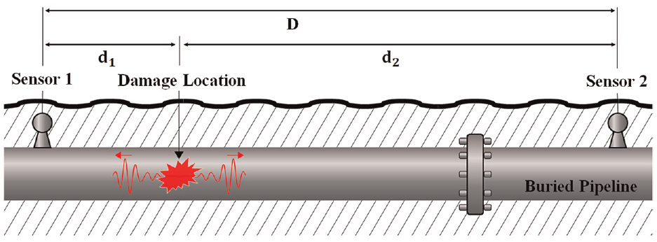
Source location in a buried pipeline with two sensors.

The TDoA-based source location can be calculated using Equation (1):

d_{1, 2} = \frac{1}{2} (D \pm c Δ t)

(1)

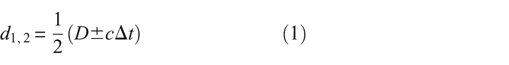
where D denotes the distance between sensors or the monitoring range, c is the propagation speed of wave, Δt is the difference in time when the wave reaches each sensor, and d_1,2 are the result of TDoA-based source location, representing the distance from the damage location to each sensor.

Among these variables, D can be determined in the sensor installation process. Therefore, an accurate source location requires accurate determination of the “wave speed” and “arrival time difference.” Thus, in this section, we describe the wave propagation speed based on the observation of fluid-filled pipeline characteristics as well as method of TDoA estimation.

Accurate determination of wave propagation speed is essential for TDoA-based source location. However, since various waves propagate through a structure and their speeds vary according to the mode, understanding the wave characteristics and selecting the appropriate mode is crucial for accurate source location. Additionally, the measurement method, which is dependent on wave mode shape, must also be considered as part of the source location process. In the case of fluid-filled pipelines, most energies are transmitted by four waves below the ring frequency.¹⁷ Here, the ring frequency is the resonant frequency of the breathing mode (n = 0), which is the fundamental vibration mode of the pipe cross-section. These waves are known to be three axisymmetric waves of breathing mode (n = 0, s = 0, 1, 2) and a bending wave (n = 1).^15,16 Among these, the fluid-borne wave (n = 0, s = 1), also referred to as a quasi-longitudinal wave, possesses lower attenuation characteristics compared to the propagation waves of structures. Hence, it has the advantage of a longer propagation distance. In addition, it can be measured easily even with a uniaxial sensor installed on the outer surface of the pipe because the interaction of fluid and elastic pipe leads to uniform contraction and expansion in all directions of the pipe cross-section. Consequently, quasi-longitudinal wave is known to be ideal for source location of buried pipelines.³²

The propagation speed of a quasi-longitudinal wave can be expressed as follows²¹:

c = c_{f} {[1 + \frac{2 B_{f} / a}{Eh / a^{2} - ρ h ω^{2}}]}^{- \frac{1}{2}}

(2)

where c _f , B _f , a, E, ρ, h, and ω denote the longitudinal wave speed of a fluid in free space, bulk modulus of the internal fluid, average radius, Young’s modulus of the pipe, density of the pipe material, pipe thickness, and angular speed, respectively.

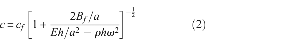
Figure 2(a) and ( b) show the dispersion curves of quasi-longitudinal waves that were calculated using Equation (2), with c _f , B _f , E, and ρ being $1500 m / s$ , $2.2 GPa$ , $200 GPa$ , and $7850 kg / m^{3}$ , respectively. Figure 2(a) depicts the characteristics of the variations in the speed of the quasi-longitudinal wave according to the frequency at various diameters. It indicates that the speed of a quasi-longitudinal wave not only depends on the frequency but also converges to 0 m/s. This finding suggests that the speed of waves propagating through a fluid in free space is constant, but quasi-longitudinal waves propagating through a fluid in a pipe may exhibit unique characteristics due to their interaction with the elastic pipe. Here, the frequency at which the speed of the quasi-longitudinal wave converges to 0 m/s is referred to as the ring frequency. Furthermore, this frequency is also that at which the wavelength of the quasi-longitudinal wave coincides with the circumference of the pipe. In other words, because the length of the circumference increases with the pipe diameter, the ring frequency of a quasi-longitudinal wave with the same wavelength decreases. Therefore, ring frequency is inversely proportional to the diameter of the pipe. Analogously, the initial speed of the quasi-longitudinal wave, which is defined as the speed at 0 Hz, is also inversely proportional to the length of the circumference of the pipe. Therefore, not only does the initial speed tend to decrease as the pipe diameter increases but it also causes a rapid change in the slope of the dispersion curve. In this study, the material properties and specifications of all pipes were in accordance with the American Society of Mechanical Engineers standard ASME B36.10M.

Figure 2.

Dispersion curve of a quasi-longitudinal wave: (a) depending on diameter and (b) depending on thickness.

Figure 2(b) is a dispersion curve that shows the initial speed change according to the pipe thickness. It represents the change in speed when the thickness of a 1200 mm pipe changes from 6 to 12 mm. In particular, it reveals a speed difference of approximately 35 m/s for every 1-mm change in thickness. This finding implies that there is a possibility of discrepancy between the theoretical propagation speed, which is calculated as the nominal thickness, and the actual propagation speed when thinning occurs due to corrosion in aging pipes. Therefore, the theoretical values through measurements of experimental propagation speed should be corrected for accurate source location.

Similar to the propagation speed, the TDoA is an important variable in source location. However, the noise generated by a real site causes difficulties in TDoA estimation. Among various approaches,^33,34 the method wherein the cross-correlation function is adopted is known to be effective for TDoA estimation in an environment with noise.^35–37 Because the cross-correlation function estimates the TDoA according to the correlation characteristics of the two signals, the noise signals, which are uncorrelated, do not contribute to the results of TDoA estimation.

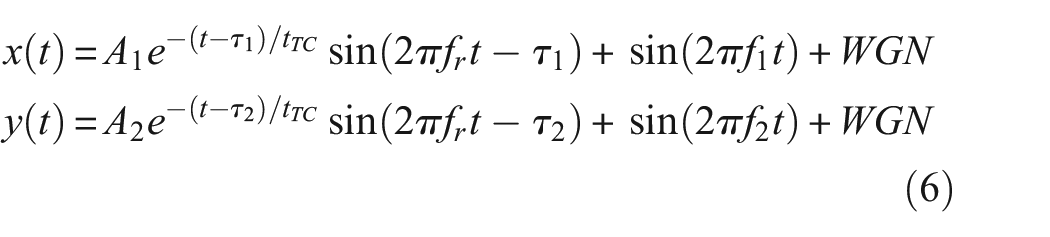
For a situation wherein impact damage occurs in buried pipelines, the measured signal can be expressed as follows³⁸:

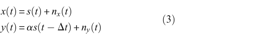
\begin{matrix} x (t) = s (t) + n_{x} (t) \\ y (t) = α s (t - Δ t) + n_{y} (t) \end{matrix}

(3)

where $x (t) and y (t)$ are the measurement signals of each sensor, $s (t)$ is the pure damage signal, $n_{x} (t) and n_{y} (t)$ are the background noise signals at each location, α is the attenuation according to the propagation distance, and Δt is the arrival time difference between the two signals.

Here, the cross-correlation for estimating the arrival time difference, $R_{xy} (τ)$ , can be expressed as follows³⁹:

R_{xy} (τ) = α R_{ss} (τ - Δ t) + R_{n_{x} n_{y}} (τ)

(4)

where $R_{ss} (τ)$ denotes the auto-correlation of damage signals included in each measurement signal, and $R_{n_{x} n_{y}} (τ)$ denotes the cross-correlation of the noise at each location.

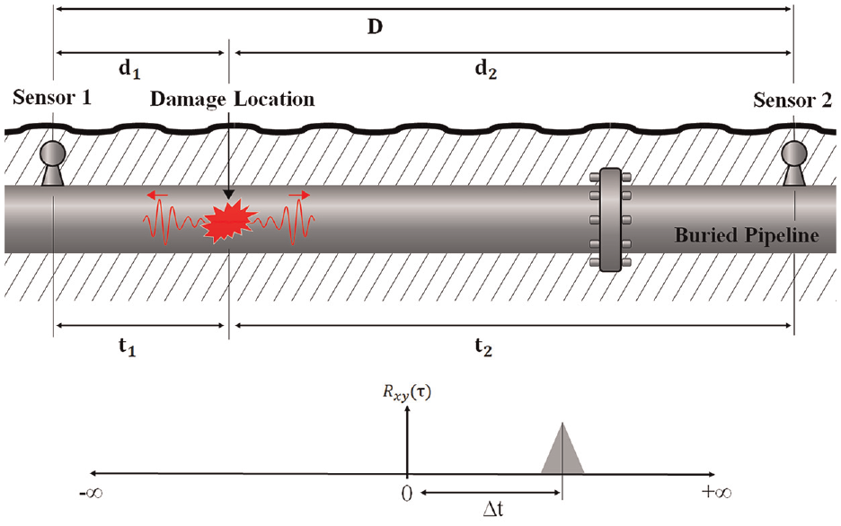
As shown in Figure 3, the result of the cross-correlation, $R_{xy} (τ)$ , represents the time-delayed auto-correlation of the damage signals. The TDoA between two signals can be estimated, as demonstrated in this figure.

Figure 3.

Source location with time arrival difference method.

Even such a cross-correlation function may provide inaccurate results when the SNR is reduced according to the noise level. To address this issue, research on enhancing TDoA estimation was conducted according to various noise characteristics. In particular, the research was undertaken to improve the cross-correlation function for leak signal detection in the in-service waterworks pipelines, and a meaningful leak detection approach was established by selecting the optimal frequency band and cross-correlation function using the window filters.³⁹ Thus, the Roth processor (ROTH),⁴⁰ smoothed coherence transform (SCOT),⁴¹ and cross-correlation function using the maximum likelihood (ML)⁴² window filters have been experimentally validated for TDoA estimation.

KTF for automatic adaptive signal processing

In this study, we newly propose a KTF to improve the performance of TDoA estimation. The role of KTF is to distinguish the hidden response of an impact damage signal included in a measured signal. Moreover, it returns a signal that is filtered to an optimal frequency band using the statistical characteristics of the impact damage signal. The main advantage of this function is the ability to bring about stable improvements in the SNR of the impact damage signal even under ever-changing noise response characteristics. Additionally, when the SNR is improved, accurate TDoA estimation is possible without the need to apply the window filter to improve the performance of the cross-correlation function as previously suggested.

To describe the theoretical background of KTF, an impact damage condition in buried pipelines was assumed, as shown in Figure 1. The impact damage that typically induces pipeline damage is produced by TPI. Therefore, the propagating wave is assumed to be a transient signal, given that it is an instantaneous impact. Here, a transient signal is defined as one whose frequency and amplitude fluctuate instantly.^43–45

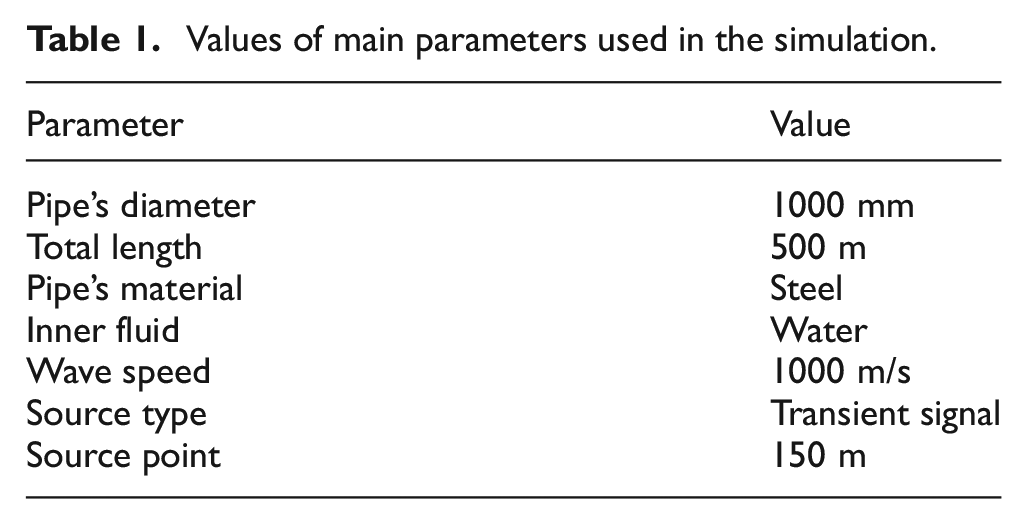
For source location, two sensors were installed at both ends of the monitoring range, as shown in Figure 1. It was assumed that the quasi-longitudinal wave generated by the unknown impact propagates in both directions. The main parameters are listed in Table 1. The diameter and total length of the pipeline were set to 1000 mm and 500 m, respectively, and the propagation speed of the quasi-longitudinal wave was 1000 m/s. Moreover, steel (ASME B36.10M) was utilized as the pipeline material, and water was used as the inner fluid. The quasi-longitudinal wave was set to propagate a distance of 150 m from sensor 1 in the form of a transient signal. Therefore, the difference in arrival time of the quasi-longitudinal waves reaching each sensor was set to be 0.2 s. Furthermore, the transient signal $S_{1} (t)$ and $S_{2} (t)$ were assumed to be a damped sine waves, as shown below:

\begin{matrix} S_{1} (t) = A_{1} e^{- t / t_{TC}} \sin (2 π f_{r} t) \\ S_{2} (t) = A_{2} e^{- t / t_{TC}} \sin (2 π f_{r} t) \end{matrix}

(5)

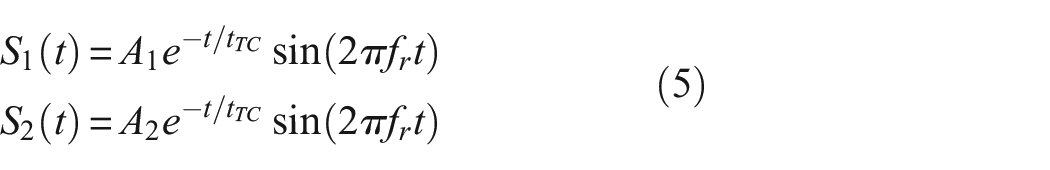
where $A_{1}$ , $A_{2}$ , $t_{TC}$ , and $f_{r}$ denote the magnitude of $S_{1} (t)$ , the magnitude of $S_{2} (t)$ , $t_{TC}$ and $f_{r}$ denote the time constant and the ringing frequency, respectively, and their values were set to be 2, 1, 0.01 s and 80 Hz, respectively.

Table 1.

Values of main parameters used in the simulation.

Parameter	Value
Pipe’s diameter	1000 mm
Total length	500 m
Pipe’s material	Steel
Inner fluid	Water
Wave speed	1000 m/s
Source type	Transient signal
Source point	150 m

To simulate the noise situation at an actual site considering propagation distance, the SNR for the virtual measurement signals were set to be −15 and −20 dB, as shown in Figure 4. The noise component consisted of a single-frequency sine wave and white Gaussian noise (WGN) because sinusoids and WGN typically contradict transient signals in terms of the time domain characteristics of signals, and mathematically clear descriptions are possible. Thus, they are suitable for observing the properties of the proposed KTF. Here, WGN is a representative random signal with an equal intensity at all frequencies, resulting in a constant power spectral density.⁴⁶ The measurement signals $x (t)$ and $y (t)$ can be expressed as follows:

\begin{matrix} x (t) = A_{1} e^{- (t - τ_{1}) / t_{TC}} \sin (2 π f_{r} t - τ_{1}) + \sin (2 π f_{1} t) + WGN \\ y (t) = A_{2} e^{- (t - τ_{2}) / t_{TC}} \sin (2 π f_{r} t - τ_{2}) + \sin (2 π f_{2} t) + WGN \end{matrix}

(6)

where $τ_{1, 2}$ denotes the time delay according to the propagation distance of each signal, and $f_{1, 2}$ denotes the center frequency of continuous noise signals.

Figure 4.

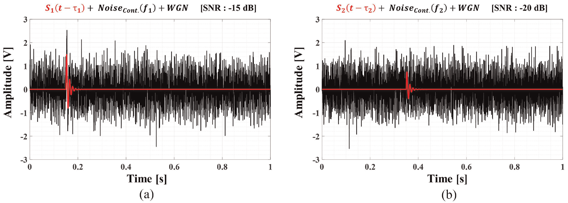
Virtual measurement signals: (a) virtual measurement signal x(t) with an SNR set at −15 dB and (b) virtual measurement signal y(t) with an SNR set at −20 dB.

Figure 4(a) shows the measurement signal x(t) of sensor 1. This signal is composed of a transient signal (ringing frequency: 80 Hz), sinusoidal noise (center frequency: 150 Hz), and WGN, with the SNR set to −15 dB. The red transient signal represents a signal that propagates a distance of 150 m from the source of damage to sensor 1 at a speed of 1000 m/s. Therefore, it takes 0.15 s for the signal to reach the position of sensor 1. Figure 4(b) presents the measurement signal y(t) of sensor 2. This signal is composed of a transient signal (ringing frequency: 80 Hz), sinusoidal noise (center frequency: 200 Hz), and WGN, with the SNR set to −20 dB. The red transient signal represents a signal that propagates a distance of 350 m from the source of damage to sensor 2 at a speed of 1000 m/s. Therefore, it takes 0.35 s for the signal to reach the position of sensor 2. Consequently, the TDoA of the transient signal included in each signal is 0.2 s.

The SNR enhancement typically emphasizes the target signal through the attenuation of noise components that exhibit different characteristics by observing the characteristics of the target signal. A bandpass filter, which is used in typical SNR enhancement methods, improves the SNR by attenuating noise components other than the main frequency band of the target signal through observation of the frequency response characteristics. Accordingly, with the aim of improving the SNR, it is necessary to observe the characteristics of the target signal. The transient signal, which was the target signal in this study, is defined by time domain characteristics such as rise time, settling time, and peak time.⁴⁷ This definition of the transient signal indicates that the signal can be classified through time-domain analysis. Here, the representative time-domain analysis method is statistical signal processing. It observes target signals based on probability distributions, which represent statistical characteristics from a probabilistic perspective.⁴⁸

Among the indicators of the probability distribution of signals, kurtosis is highly suitable for expressing the characteristics of transient signals.⁴⁹ In this connection, Dwyer proposed frequency domain kurtosis (FDK) to detect transient signals that are generated by ice cracks. Furthermore, it was demonstrated that the FDK is more effective in detecting transient signals than the power spectrum density, which is a representative indicator for the observation of signal characteristics.^50,51 Consequently, in this article, we newly propose a KTF-based source location method to improve the TDoA estimation performance of the cross-correlation function by improving the SNR of the noisy signal using kurtosis.

In probability theory and statistics, kurtosis is a measure of “tailedness” in probability distributions of random variables. In other words, kurtosis is a measure of the probability distribution shape of a signal. Pearson defined kurtosis as the fourth moment of a probability distribution, as shown below⁵²:

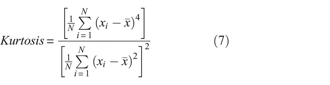
Kurtosis = \frac{[\frac{1}{N} \sum_{i = 1}^{N} {(x_{i} - \bar{x})}^{4}]}{{[\frac{1}{N} \sum_{i = 1}^{N} {(x_{i} - \bar{x})}^{2}]}^{2}}

(7)

where $x_{i}$ is the $i$ -th sample, $\bar{x}$ is the mean, and N is the number of samples.

Many scholars have defined kurtosis as a measure of the degree of sharpness of a probability distribution or the degree to which the data are concentrated at the center. However, a more precise and accurate definition is that it is a measure of the tail of a probability distribution.^53,54 In other words, the higher the kurtosis of the measurement signal, the longer (or light) the tail on the probability distribution. Therefore, transient signals, which have larger variations in amplitude than steady-state signals such as WGN, are expected to have higher kurtosis values. The property of having higher kurtosis values for transient signals, which exhibit larger amplitude variations compared to steady-state signals like WGN, can be used to differentiate them from steady-state signals by examining their kurtosis. In a normal distribution, kurtosis has a value of 3, and WGN serves as a representative example of a normal distribution signal. As a result, if the kurtosis value of a measured signal exceeds 3, it is highly likely that the measured signal is a transient signal. Additionally, a sine wave, characterized by more extreme values than median values in its probability distribution, displays a concave probability distribution and has a kurtosis of 1.5.

To obtain the KTF proposed in this study, the kurtosis response (f) must be calculated beforehand to improve the SNR of the hidden transient signal within a noisy signal using the kurtosis characteristics described previously. The kurtosis response (f) can be expressed as follows:

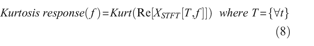
Kurtosis response (f) = Kurt (Re [X_{STFT} [T, f]]) where T = {\forall t}

(8)

where T denotes the set of time elements corresponding to each frequency in the two-dimension array of short-time Fourier transform (STFT) and f denotes each frequency component.

In other words, kurtosis response (f) indicates the kurtosis of the real part for the total time per frequency after converting the measurement signal into a two-dimensional array using STFT. Thus, it shows a high kurtosis response level only in the frequency band where the transient signal exists. Here, only the real part of the STFT, which is a complex number, is used. Because the kurtosis response (f) is only important in the magnitude response, the imaginary numbers are determined to be unnecessary and can be discarded. As usual, the real part of the complex number is used to compute the magnitude of the component, and the imaginary part is used to compute the phase angle.

Figure 5 shows the process for calculating the kurtosis response (f) using the measurement signal of sensor 1, as assumed previously. This signal is a mixture of transient signal, continuous signal, and WGN, as seen in the STFT result. The kurtosis response (f), which is the kurtosis for the total time per frequency, is 19.5 in the 80 Hz band in which transient signals exist, 1.5 in the 150 Hz band in which continuous signals exist, and 2.9 in the 250 Hz frequency band in which only the WGN exists. Figure 6(a) shows the kurtosis response (f), which was obtained by arranging these values in order of frequency. These results exhibit different characteristics from the frequency response characteristics calculated by fast Fourier transform shown in Figure 6(b). Here, it can be seen that the 150 Hz band, which represents a high level in the frequency response, appears as a low level in the kurtosis response (f). In particular, even though a transient signal cannot be distinguished by the frequency response characteristics, the signal can be distinguished because it appears at the highest level in the kurtosis response (f). Moreover, as described previously, WGN represents a value close to 3. Based on the observation of characteristics using such kurtosis, a frequency band wherein transient signals are prominent can be selected without the need for an artificial frequency band selection process.

Figure 5.

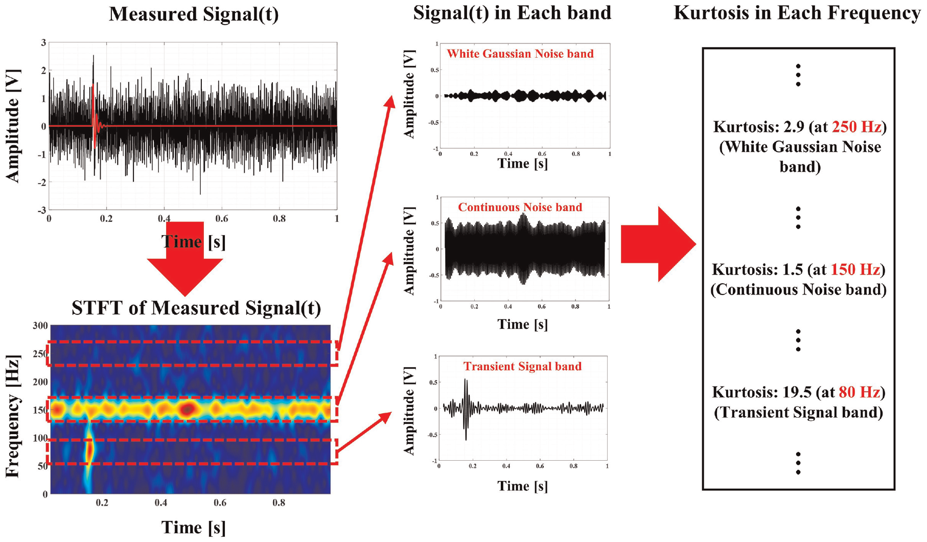
Process for calculating the kurtosis response (f).

Figure 6.

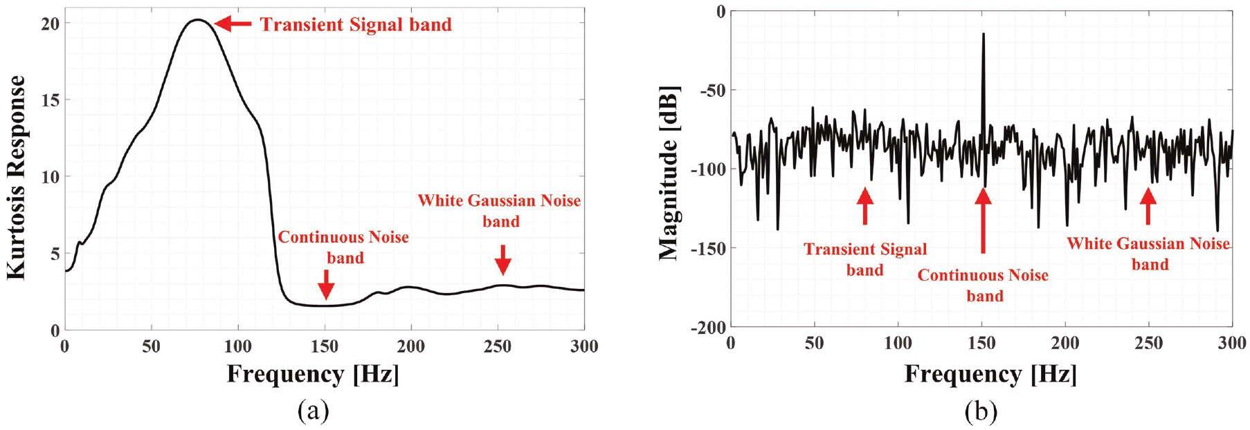
Comparison of kurtosis response and frequency response calculated by the virtual measurement signal x(t): (a) kurtosis response and (b) frequency response.

Because source location in buried pipelines is performed using two sensors, which are installed at both ends of the monitoring range, the KTF proposed in this study can be determined by calculating the kurtosis response (f) for the two signals, as shown below:

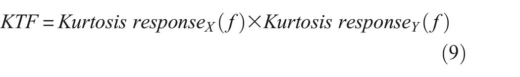
KTF = Kurtosis respons e_{X} (f) \times Kurtosis respons e_{Y} (f)

(9)

Figure 7 shows the results of calculating the KTF using the signals in Figure 4. A relatively high response level is observed in the 80 Hz band, which is the target signal for SNR improvement, whereas a low response level can be observed in the 150 and 200 Hz bands, which consists of noise signals. These results indicate that the SNR of a target signal can be improved without artificially selecting an optimal frequency band through observation of the statistical characteristics of the signal. The KTF can ensure a high response level of the impact damage signal despite the variations in the optimum frequency band according to the characteristics of the background noise. This characteristic may also enable widespread use in field applications.

Figure 7.

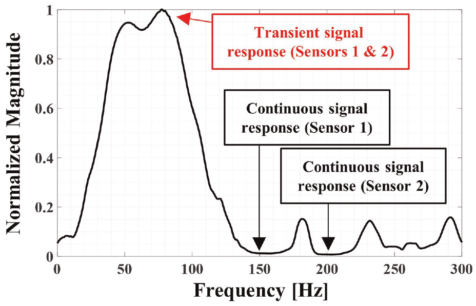
KTF results for transient and continuous signals considered in the simulation.

Finally, a signal with an improved SNR for TDoA estimation can be obtained from the inverse fast Fourier transform (IFFT) to which the KTF is applied. In this case, the KTF was calculated without considering the phase information. However, when performing the IFFT process, which applies the KTF, the phase information related to the raw signal is utilized. The following equation represents the process of reconstructing a signal by applying the KTF to the frequency response characteristics of the raw signal:

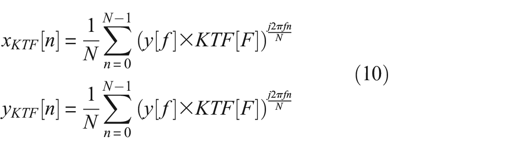
\begin{matrix} x_{KTF} [n] = \frac{1}{N} \sum_{n = 0}^{N - 1} {(y [f] \times KTF [F])}^{\frac{j 2 π fn}{N}} \\ y_{KTF} [n] = \frac{1}{N} \sum_{n = 0}^{N - 1} {(y [f] \times KTF [F])}^{\frac{j 2 π fn}{N}} \end{matrix}

(10)

where $x_{KTF} [n]$ and $y_{KTF} [n]$ represent processed signals, which are the IFFT results of the raw signals to which KTF has been applied. Here, a discrete-time expression was employed here.

The results of signal reconstruction using the KTF are shown in Figure 8(a) and (b). The transient signal can be clearly distinguished, unlike for the signal shown in Figure 4. Furthermore, the frequency response of the processed signals in Figure 8(c) and (d) indicate an improvement in the SNR based on the attenuation of the frequency response other than in the 80 Hz band of the transient signal. In particular, the responses of the 150 and 200 Hz bands, which consist of the continuous signal, are decreased by approximately 100 dB compared to the raw signal. Here, 100 dB is a slightly exaggerated value because it is a simulation result. These results indicate that when the KTF is used in source location of buried pipelines, the SNR of the hidden transient signal can be improved without selecting an optimal frequency band. However, when applying the KTF, a transient signal and a continuous signal (consisting of the sum of various frequencies) cannot be distinguished from each other if they exhibit perfectly identical frequency response characteristics.

Figure 8.

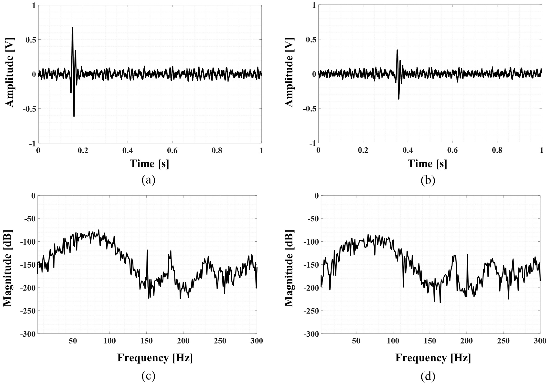
Time signal and its frequency response with applied KTF: (a) time signal of $x_{KTF} [n]$ , (b) time signal of $y_{KTF} [n]$ , (c) frequency response of $x_{KTF} [n]$ , and (d) frequency response of $y_{KTF} [n]$ .

To verify the effect of the KTF, the cross-correlation results obtained by applying the aforementioned effective windowing filter were compared. The comparative windowing filter was composed of ROTH, SCOT, and ML, whose performance was verified, as described in section “Theoretical background of source location.”

Figure 9 shows the result of cross-correlation using the KTF. From the figure, it can be seen that the calculated TDoA accurately represents the designed delay time of 0.2 s. Figure 10(a) presents the result of the window filter-based cross-correlation calculated using the raw signal. Figure 10(b) shows the window filter-based cross-correlation results calculated using the signal filtered with the optimal frequency band of 80 Hz. It can be observed that the window filter, known to be effective in determining TDoA, cannot be used to estimate TDoA at the SNR level of −20 dB. Moreover, it was confirmed that TDoA estimation is possible only when the signal is filtered using the optimal frequency band. This finding suggests that the process of selecting the optimal frequency band is important in TDoA estimation, as described previously. However, because the optimal frequency band is defined as the one with a high SNR, the optimal frequency must be re-selected every time in a practical environment in which the response characteristics of the noise constantly change. Therefore, the approaches for artificially selecting an optimal frequency band cannot be easily implemented in practical fields. However, the KTF proposed in this study may be seamlessly implemented in actual applications because it can effectively improve the SNR of the impact damage signal.

Figure 9.

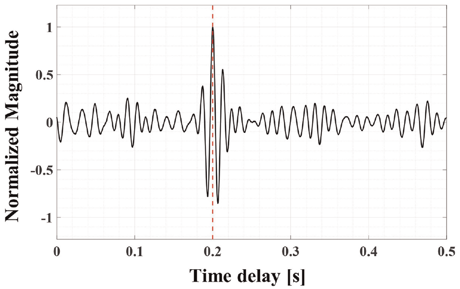
Result of time delay estimation using KTF-based cross-correlation.

Figure 10.

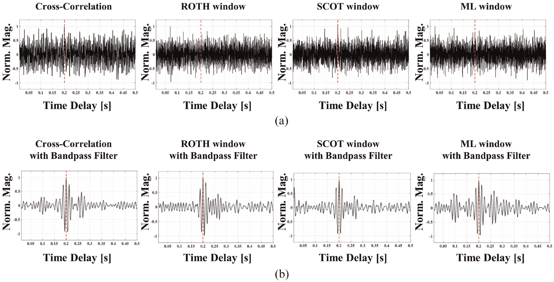
Comparison of window filter-based cross-correlation results: (a) results of cross-correlation using raw signal and (b) results of cross-correlation using filtered signal.

Anomaly detection algorithm for decision of impact damage occurrence

For failure prevention through early detection of impact damage in buried pipelines, both the source location and anomaly detection are essential, because as described previously, for impact damage that occurs unexpectedly due to external interference, the optimal way to prevent damage is to respond early through determination as quickly as possible. However, the impact damage cannot be determined based on the results of source location alone, because the TDoA, which corresponds to the maximum of the cross-correlation function, can be calculated for any signal independent of the impact damage.

In this study, we propose a new monitoring algorithm for buried pipelines based on the source location and anomaly detection for impact damage, as illustrated in Figure 11. Source location is performed using the cross-correlation function to which the KTF is applied. The anomaly detection consists of binary classification wherein two features are selected from the measured signal, and they are considered as damage only when they are above the specified threshold simultaneously. In other words, if both features 1 and 2 simultaneously exceed the threshold value that has been set in advance, the source location results reflect the actual impact damage. Conversely, if one of the features being below the threshold value, it indicates the normal state. This binary classifier-type algorithm helps determine the occurrence of impact damage, even though it cannot determine the degree of damage. Therefore, it can effectively prevent damage and be used to implement immediate response measures for inaccessible structures such as buried pipelines.

Figure 11.

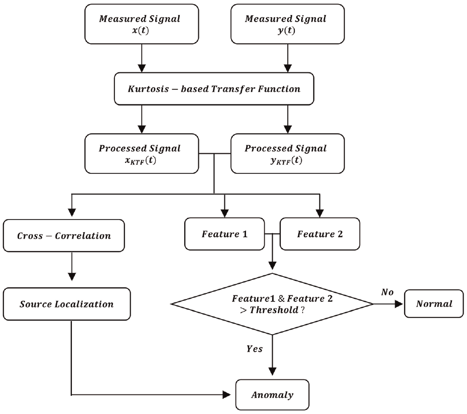
Monitoring algorithm for buried pipelines.

For the anomaly detection of impact damage in the pipelines, we selected two features that represents the characteristics of the impact damage signal in the time and frequency domains. The first feature, $F_{k}$ , is calculated using kurtosis and represents the characteristics of the transient signal in time domain described in section “KTF for automatic adaptive signal processing.” The second feature is the newly proposed modified magnitude-squared coherence index MMSC_index, which represents the frequency domain similarity between the transient signals. If both of these features exceed the predetermined threshold value, it is probable that the measured signals are both transient signals and exhibit a high degree of similarity in their frequency responses. In contrast, when $F_{k}$ is above the threshold and MMSC_index is below the threshold, noise from unknown sources appears in the form of a transient signal. However, because there is no mutual similarity, the state of the pipelines is determined to be normal. In contrast, when the similarity of the two signals is high due to continuous noise and the signal is not caused by impact damage, the state is determined to be normal. A few representative examples of this include electrical noise and system noise. Furthermore, when both features are below the threshold value, the state is determined to be normal.

As described in section “KTF for automatic adaptive signal processing,” the first feature, F _k , is calculated using kurtosis and represents the characteristic of the transient signal. However, it is necessary to convert two kurtosis values into one feature because two signals are measured during the monitoring of impact damage of buried pipelines. Thus, the two signals were normalized and reconstructed into one signal, and the calculated kurtosis was represented as F _k , as illustrated in Figure 12. The results confirmed that the value of F _k is relatively high only when the impact damage signal simultaneously exists in both signals. Here, the use of the arithmetic average of kurtosis, referred to as the mean of kurtosis in Figure 12, is equivalent to the F _k value when both signals contain only impact damage or noise. However, when two types of signals are mixed, the arithmetic average is approximately twice as high as F _k . Additionally, the arithmetic average of a mixed signal is three times higher than a signal that consists only of noise, even in the same normal state. Conversely, the F _k value of a mixed signal is less than twice as high as that of a signal that consists only of noise. Consequently, the arithmetic average is unsuitable due to the high possibility of mis-determination. In this case, the reference value of F _k is 3, which is the kurtosis value of WGN. For impact damage signals, the processed signals shown in Figure 8 were utilized.

Figure 12.

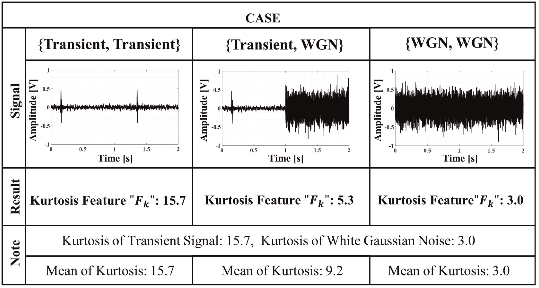
Kurtosis feature results in each case.

The second feature, MMSC_index, was inferred from the error that is induced when magnitude-squared coherence (MSC), which represents the similarity of two signals, is applied to a transient signal. The MSC is obtained from the similarity estimation function, coherence, of the two signals that adopt the Welch’s method, wherein a signal is divided into multiple segments and analyzed for accurate estimation of the signal response. This is inaccurate in the similarity estimation results because a signal exists only in a specific segment when applied to a transient signal, although it always exhibits high similarity in the case of a sinusoid, where signals exist in all segments when a specific signal is divided into multiple segments.⁵⁵ Therefore, the frequency domain similarity of the transient signals can be measured if the transient signals are aligned such that they are located in the same segment. In other words, in the case of the impact damage signal, the exact similarity response characteristics can be observed only when signal alignment is performed first.

Figure 13 shows the results of MMSC aimed at calculating the MMSC_index feature proposed in this study. Figure 13(a) depicts the signal of sensor 1, which is the specified standard for signal alignment. Figure 13(b) presents the signals before and after the time alignment of the signal from sensor 2. Here, the signal alignment uses the TDoA obtained in section “KTF for automatic adaptive signal processing.”Figure 13(c) compares the MSC results before and after time alignment. The time alignment results in a difference in the similarity response of 80 Hz, which is the center frequency of the transient signal. The MMSC_index feature proposed in this study can be calculated from the difference between the two MSCs obtained using this approach, as shown in Figure 13(d). If the MSC before time alignment is $γ^{2}$ and that after time alignment is $β^{2}$ , the MMSC can be calculated from the difference between the two MSCs. Although the conventional MSC represents the similarity as a normalized value between 0 and 1, the value of MMSC is between −1 and 1. Furthermore, MMSC_index uses the arithmetic mean of the ±α band based on the maximum response frequency of the KTF obtained previously. Consequently, the value of MMSC_index is close to 1 in the event of an impact causing pipeline damage. However, the value is close to 0 when only WGN exists. In contrast, if it is close to −1, each signal has noise in the form of a transient signal at the same time, but it is shifted to different times after time alignment. On the other hand, MMSC_index converges to 0 in the case of electrical noise, such as 60 and 120 Hz, which has a high probability of occurring in practical applications.

Figure 13.

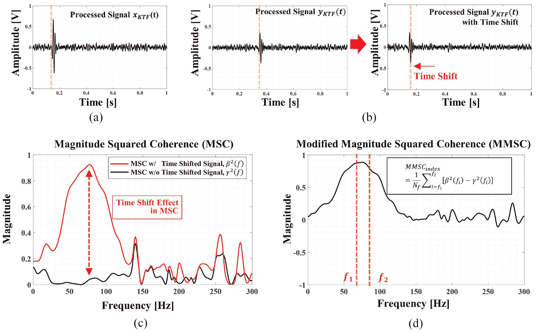
Process for calculating the MMSC_index: (a) processed signal $x_{KTF} (t)$ as standard for signal alignment, (b) processed signal $y_{KTF} (t)$ before and after alignment, (c) comparison of MSC results before and after signal alignment, and (d) MMSC results for MMSC_index.

Since the source location provides estimation results regardless of whether they are damaged, it is important to determine whether it stems from the impact damage. Thus, we observe F _k , which represents the probability of transient signals in the time domain, and MMSC_index, which represents the similarity of transient signals included in the measurement signal in the frequency domain. The anomaly detection algorithm illustrated in Figure 11 can be implemented accordingly. In particular, Figure 14 shows the calculation results for MMSC_index and F _k when the impact signal occurs and in a normal state. Figure 14(a) demonstrates that MMSC_index and F _k are 0.8828 and 22.7, respectively, when there is an impact signal. In Figure 14(b), MMSC_index and F _k are 0.0953 and 3.0, respectively, in the normal state.

Figure 14.

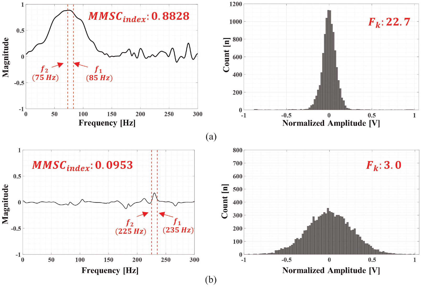
MMSC and F _k results or anomaly detection: (a) using transient signal and (b) using WGN signal.

The two values calculated using this approach are expressed as a scatter plot in Figure 15. In this way, pipeline anomaly detection could be implemented by distinguishing the anomaly state expressed in the red area and the normal state in the green area. If both MMSC_index and F _k exceed the threshold, the state is an anomaly; in all other cases, it is normal.

Figure 15.

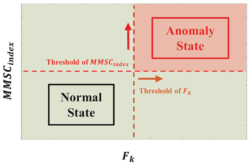
Scatter plot for anomaly detection using two features.

Experimental verification

Experimental setup

In this study, experimental verification was performed on an aging buried waterworks in-service pipeline with a large diameter with the aim of verifying the proposed impact damage monitoring algorithm, as shown in Figure 16(a) and (b). The pipelines to be tested were a steel pipeline of diameter 1200 mm and length 564 m. The impact damage situation was reproduced at the 136 m position using an impact hammer (sensitivity: 0.225 mV/N). In the case of sensor 1, a quasi-longitudinal wave propagating at 136 m was measured, and in the case of sensor 2, a quasi-longitudinal wave propagating at 428 m was measured. Furthermore, to measure the impact signal, an accelerometer (sensitivity: 10 V/g) was installed in an accessible valve chamber, shown in Figure 17(a), by using a magnetic base, depicted in Figure 17(b). We used the NI-9234 model (National Instruments, USA) and measured the signals with a sampling frequency of 5.12 kHz. The test was conducted in an environment with various noises because the target pipeline was buried under a round-trip eight-lane roadway and a parking lot.

Figure 16.

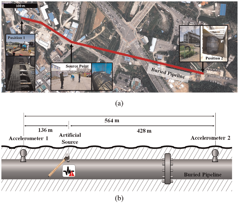
Schematics for experiments: (a) pipeline layout on map and (b) positions of sensor and artificial source.

Figure 17.

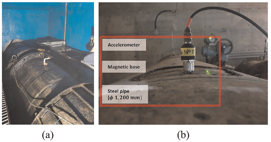
Experimental setup: (a) typical valve chamber of waterworks pipelines (diameter = 1200 mm) and (b) accelerometer installation using magnetic base.

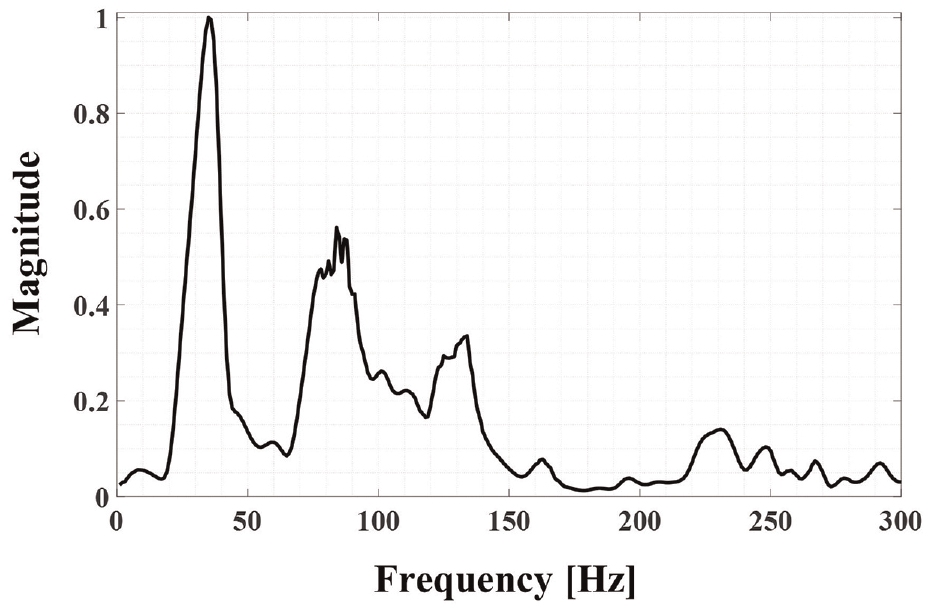
As mentioned in section “Theoretical background of source location,” the propagation speed of a quasi-longitudinal waves varies according to its frequency. This inaccurate propagation speed lead to false errors in source location. Therefore, to minimize these errors, the probability of false detection was minimized by assuming that the quasi-longitudinal wave was a non-dispersive wave through the observation frequency band constraint, as shown in Figure 18. Here, the observation frequency band was selected as 300 Hz, which represents a speed of 951.1 m/s. This speed differs by −1.5% from the propagation speed of 966.3 m/s at 0 Hz. In other words, the quasi-longitudinal wave was assumed to be a non-dispersive wave with a propagation speed of 958.7 m/s. A speed difference of approximately 15 m/s between 0 and 300 Hz represents an error range of approximately 1 m in the source location outcome.

Figure 18.

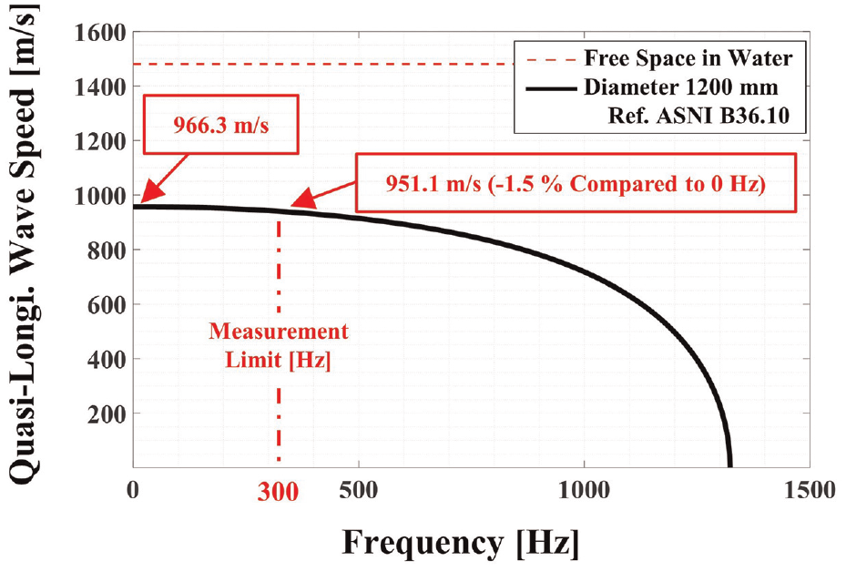
Observation frequency band constraint used to assume a non-dispersive wave.

Experimental method

We performed two experiments to verify the feasibility of the proposed algorithm. First, a preliminary experiment was conducted to measure the propagation speed of a quasi-longitudinal wave. As mentioned previously, this step was aimed at compensating for the error between the theoretical propagation speed and the experimental propagation speed caused by the aging of the pipelines and inaccurate thickness information, even in cases where it is assumed that the propagation speed is constant regardless of the frequency. An impact hammer was used as an artificial source with an impact strength of approximately 45 kN, as shown in Figure 19(a). The optimal frequency band for SNR improvement was established through observation of the frequency response characteristics and coherence, which is a well-known method. As depicted in Figure 16(b), sensors were installed at both ends of a pipeline of length 564 m. The pipeline was directly excited using an impact hammer as an artificial source at a location with a distance of 136 m. Sensor 1 measures the quasi-longitudinal wave propagating through the pipeline at a position situated at a distance of 136 m to the left of the source within the impact, and sensor 2 measures that at a position situated at a distance of 428 m to the right of the impact source. Additionally, the optimal frequency band selection results derived from the preliminary experiment were compared with the results obtained using the KTF proposed in this study, and the results were used to verify the performance of the KTF.

Figure 19.

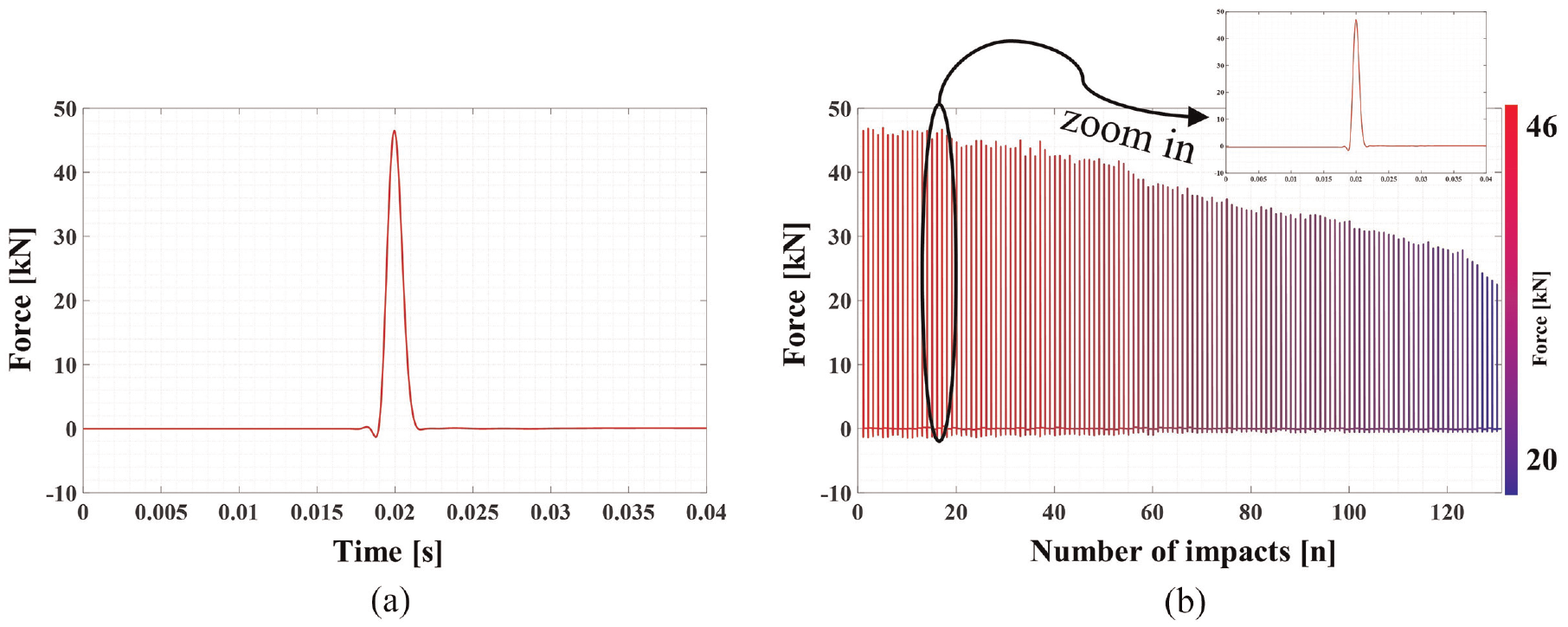
Impact signals for each damage test: (a) typical impact signal and (b) impact signals with various strengths.

Impact damage situations of various strengths were reproduced to monitor the impact damage in this experiment, as shown in Figure 19(b). The results of the proposed algorithm for source location and anomaly detection were experimentally verified. Moreover, to verify the performance in various noise settings, experiments were conducted at three time: during rush hour (17:00), in the evening (22:00), and at midnight (24:00). During rush hour (17:00), the noise is high due to increased commuting traffic; in the evening (22:00), the noise is relatively low; and at midnight (24:00), the noise is significantly less frequent as there are fewer people. Furthermore, the impact strengths were reproduced within the range of 20–46 kN, 75, 110, and 130 times at the rush hour, evening, and midnight times, respectively. Based on these outcomes, we aimed to verify the performance of the proposed algorithm.

Result and discussion

Quasi-longitudinal wave speed verification

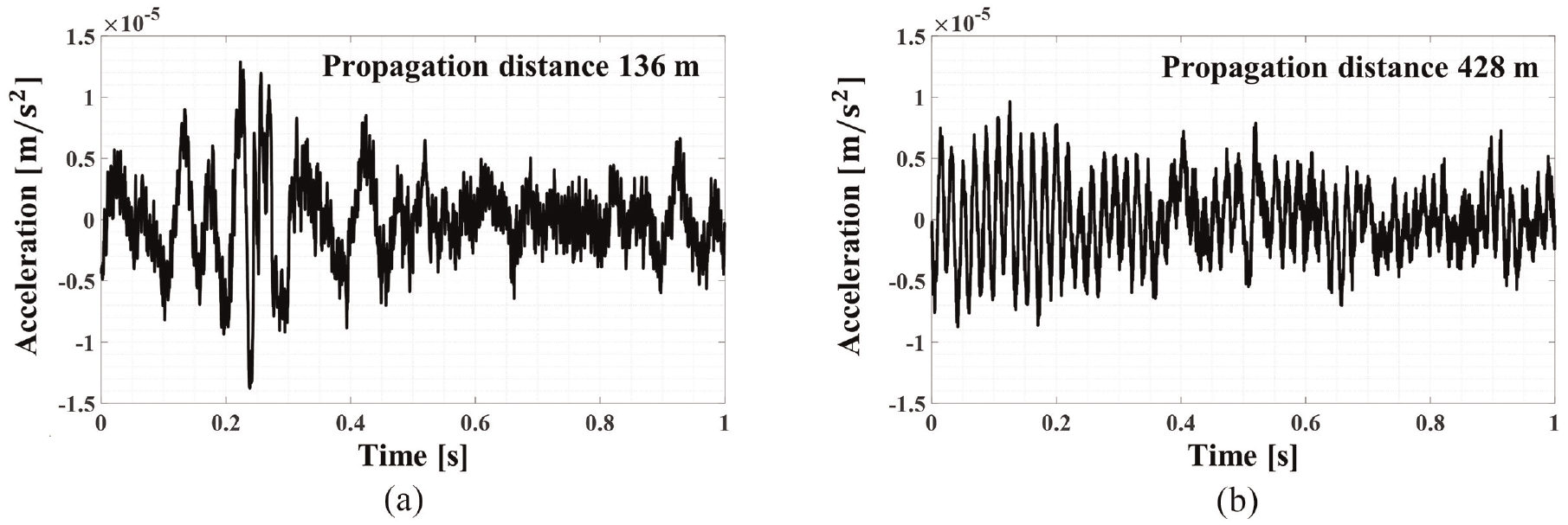
Prior to this experiment, another experiment was conducted to measure the propagation speed of a quasi-longitudinal wave. The artificial source was excited a total of 10 times with a strength of approximately 45 kN at a position situated at a distance of 136 m out of the total distance of 564 m. Figure 20(a) and (b) show signals that were propagated at 136 and 428 m, respectively. The signal propagated at 428 m has a relatively low signal level due to attenuation based on the propagation distance. Because the difference between the levels of these signals also causes a difference in frequency response, it is necessary to select a frequency band with a high SNR and similarity as the optimal frequency band for both signals. Figure 21 presents the results of selecting the optimal frequency band, and Figures 21(a) and (b) compare the vibration acceleration level result of the impact signal and the background noise signal of each signal. Figure 21(c) shows the MSC results for the frequency band with a high similarity between the two signals. As depicted in Figure 13(b), the MSC was calculated after time shifting the impact signal to the same segment.

Figure 20.

Time signals obtained from each sensor: (a) sensor 1 and (b) sensor 2.

Figure 21.

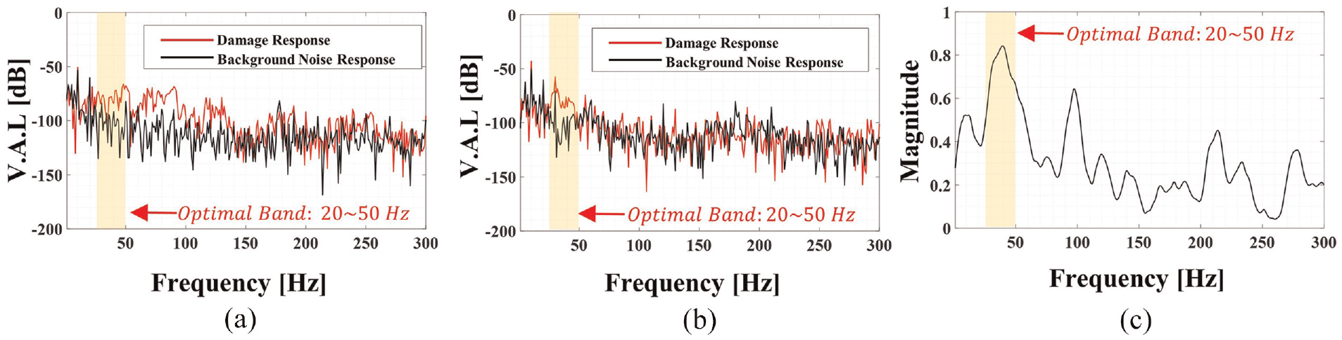
Frequency response obtained from each sensor and MSC results: (a) comparison of frequency response of sensor 1 (damage signal and background noise), (b) comparison of frequency response of sensor 2 (damage signal and background noise), and (c) MSC results calculated using each damage signal.

Consequently, as shown in Figure 21(a), a wide band of high SNR compared to background noise was found below 300 Hz in the frequency response of the signal that propagated for 136 m. In contrast, in the frequency response of the signal that propagated 428 m in Figure 21(b), the level of the impact signal was higher than that of the background noise signal in the 20–50 Hz band. Furthermore, Figure 21(c) provides the MSC results of the two signals, indicating that there is high similarity in the band 20–50 Hz compared to the other frequency bands. From these results, the optimal frequency band was selected as approximately 20–50 Hz. Figure 22 shows the signals filtered to the optimal frequency band, and Figure 23 presents the results of cross-correlation using these signals.

Figure 22.

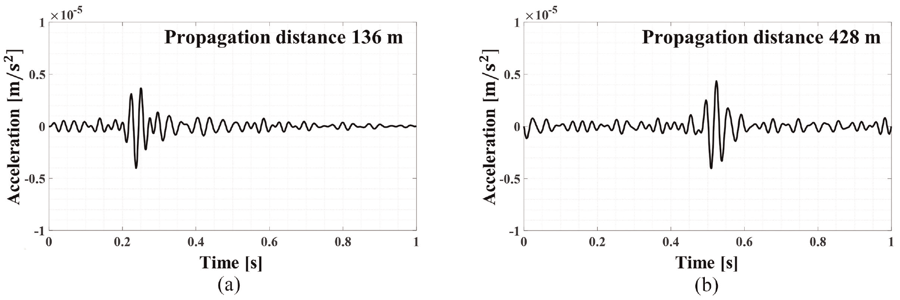
Time signal obtained after optimal bandpass filter process: (a) sensor 1 and (b) sensor 2.

Figure 23.

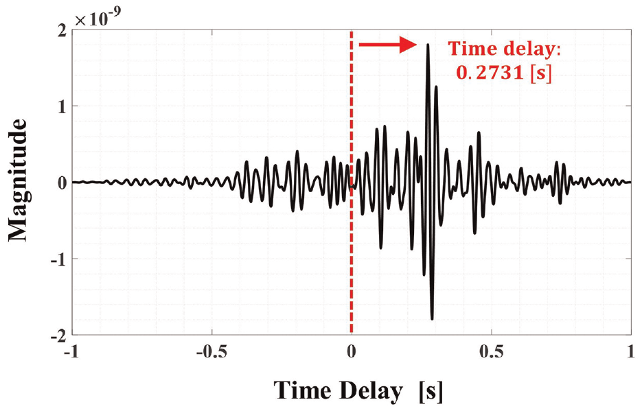
Cross-correlation for the filtered signals.

The TDoA between the two signals was approximately 0.2731 s. The propagation speed of the quasi-longitudinal wave calculated using this TDoA was 1069 m/s. Table 2 outlines the results of the propagation speed estimation experiment that was repeated 10 times. When filtering with the optimal frequency band, the average speed was 1067.5 m/s and the standard deviation was 7.12 m/s, indicating a relatively constant speed. In contrast, when the propagation speed was calculated according to the raw signal, the average was 1930.6 m/s and the standard deviation was 2165 m/s. These results confirm that even with the same impact intensity, speed measurement is almost impossible if it is not filtered according to the optimal frequency band.

Table 2.

Comparison of estimated wave speed for raw signal and that after optimal bandpass filtering.

Test no.	Estimated wave speed
Test no.	w/o bandpass filter (m/s)	w/ bandpass filter (m/s)
1	963	1070
2	966	1069
3	6795	1067
4	1071	1068
5	973	1069
6	332	1066
7	1070	1067
8	959	1065
9	1075	1068
10	5102	1066
Mean value	1930.6	1067.5
Standard deviation	2165	7.1
Theoretical value	958.7

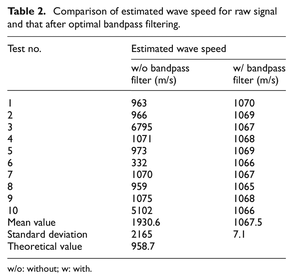
w/o: without; w: with.

The preliminary experiment introduced in section “Quasi-longitudinal wave speed verification” revealed that the theoretical propagation speed of the quasi-longitudinal wave was 958.7 m/s, whereas the experimentally obtained propagation speed was approximately 1067 m/s. These results suggest that the difference is caused by the effect of the buried environment that was not considered in the theoretical value and the inaccurate thickness information described previously.

Source location in waterworks pipelines

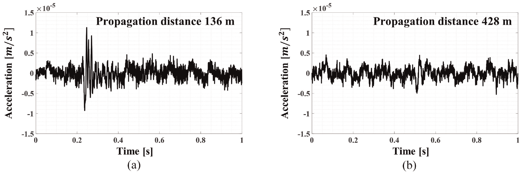
In this experiment, the source location performance of cross-correlation using the KTF was verified under various noise conditions, as described in section “Experimental method.”Figure 24(a) and (b) show the signals that propagated for 136 and 428 m, respectively, through an impact of approximately 45 kN. In particular, in actual buried pipeline damage monitoring, the SNR is reduced when contaminated with various noises, as shown in Figure 24(b). Therefore, the effect is not likely to be significant even in the optimal frequency band obtained in section “Quasi-longitudinal wave speed verification.”

Figure 24.

Time signals obtained from each sensor: (a) sensor 1 and (b) sensor 2.

In such a variable-noise environment, it is difficult to select the optimal frequency band for source location. Moreover, a situation wherein the optimal frequency band changes due to noise may occur even if the optimal frequency band is selected. To address this issue, the KTF, which can return the optimal frequency band based on statistical characteristics, was proposed in this study, and the results are shown in Figure 25.

Figure 25.

KTF results calculated using raw signals.

The optimal frequency band obtained using the KTF is 30–40 Hz, which is highly similar to the manually derived optimal frequency band in Figure 21. Furthermore, as shown in Figure 26, the TDoA estimated from the cross-correlation using the KTF was 0.2734 s. A difference of approximately 0.0003 s is seen compared to the cross-correlation results of the signals filtered with the optimal frequency band manually obtained in the previous section. This difference corresponds to 0.158 m in the source location results. In other words, the KTF enables source location through the identification of the optimal frequency band for impact damage source location without the need for an additional optimal frequency band selection process. Therefore, it was experimentally verified that this method is suitable for impact damage monitoring of facilities with various noises, such as in-service buried pipelines.

Figure 26.

Cross-correlation for the processed signals by KTF.

Figure 27 presents the source location results according to the impact strength under various noise conditions. Here, each point represents one impact experiment, and the x- and y-axes represent the results of source location and the number of impact experiments, respectively. The color indicates the impact strength in the range of 20–46 kN. Figure 27(a) shows the results of the experiment conducted during rush hour (17:00) when the background noise level was high. A total of 75 different impact strengths were simulated. For the impact strength of 45 kN, there was a possibility of frequent error in the source location results. For an impact strength of approximately 20 kN, highly inaccurate results were obtained. However, source location was found to be feasible with relatively high accuracy at impact strengths equal to or greater than 30 kN. Figure 27(b) provides the results of 110 impact strength experiments conducted in the evening (22:00), when the frequency of noise occurrence is relatively low. These results confirm that accurate source location is possible in most strength, including those with an impact strength of approximately 20 kN, contrary to the results obtained during rush hour. Here, the actual impact position was situated at a distance of 136 m, but the results of for the location at 125 m appeared intermittently due to an error in the cross-correlation calculation process. An error of approximately 10 m occurred even with an error of one wavelength because a low frequency with a longer wavelength was used.

Figure 27.

Results of source location according to the impact strength at different times: (a) rush hour (17:00), (b) evening (22:00), and (c) midnight (24:00).

Figure 27(c) shows the results of the impact strength experiment conducted at midnight (24:00), when the possibility of contamination due to background noise is very low. A total of 130 impact experiments were performed. More accurate analysis was possible, particularly because the frequency of occurrence of noise was remarkably low. Therefore, it was experimentally verified that accurate source location can be achieved with a high probability by utilizing the KTF when an impact occurs in a buried pipeline. In addition, the location of damage was calculated as the point at a distance of 136.14 m, which is extremely close to the actual impact position. This finding experimentally verified the source location performance of the KTF proposed in this study. Considering that the external impact (e.g., TPI) in actual situations is approximately several hundred kilonewtons, the KTF showed an excellent detection rate in most time slots. Furthermore, in an environment with a high frequency of noise occurrence, even if the accuracy is decreased, a stochastically constant source location result may be yielded when a continuous impact damage signal such as TPI occurs. This characteristic suggests that the KTF is suitable for actual field applications. However, even with the same impact strength, the fact that different results are obtained depending on the background noise situation suggests the need for improvement of the proposed KTF. In particular, the cross-correlation applied in this study used a basic function with no window filter. Therefore, it is expected that better detection performance will be possible if a window filter suitable for impact damage monitoring could be derived through signal analysis in the future.

Anomaly detection and performance evaluation

In the context of impact damage monitoring for buried pipelines, it is important to determine whether a detected signal is the result of actual impact damage, even when the location of the damage has been identified. Thus, we classified the results of source location into normal and anomalous results by using the proposed algorithm in Figure 11. Figure 28(a) and (b) present the MMSC_index and F _k results calculated using the noise-contaminated impact damage signals in Figure 24. Figure 28(a) shows the MMSC results, which indicate the similarity between the two signals. Similar to the KTF calculated previously, a high response in the 30–40 Hz band is observed. In particular, the average MMSC_index value in the frequency band showing the maximum KTF is 0.74. This finding suggests that the corresponding frequency band has a high similarity of impact damage signals. Furthermore, the kurtosis calculated using the probability distribution of the signal shown in Figure 28(b) is 16.82. Because this value is greater than 3, which is the kurtosis value of the normal distribution, it is likely that the signal is an impact signal. This finding suggests that the source location result of 136.14 m obtained in section “Source location in waterworks pipelines” is due to impact damage.

Figure 28.

Result of monitoring features calculated by impact signals: (a) MMSC results for the similarity measure in the frequency domain and (b) probability distribution results to determine the damage possibilities in the time domain.

Figure 29 compares the anomaly detection results according to various impact intensities and the background noise results in each time slot. Figure 29(a) and (b) show the anomaly detection result for each impact strength and those obtained using only the background noise, respectively. In the results of the experiment performed during rush hour (17:00), when various noises are likely to occur due to the increase in traffic volume, the boundary between the impact group and the background noise group is very close. In particular, in the case of impact strength close to 20 kN, which is indicated by blue dots, the MMSC_index and F _k values are close to 0.2 and 4, respectively, which are similar to the values obtained using only background noise. Even in the case of impact strength of 40 kN or more, most of the results are distinguishable from those acquired with background noise. In the case of evening (22:00), as the impact strength increases, the MMSC_index and F _k values form clusters at 0.5 and 15, respectively. A comparison of these results with those obtained during rush hour (17:00) reveals that the proposed algorithm is somewhat dependent on background noise. Similarly, in the case of the midnight (24:00) results, which are not affected by noise, it shows high accuracy in distinguishing most the impact damage compared to background noise. In particular, the red dots representing the impact strength of approximately 40 kN indicate high clustering in most time slots.

Figure 29.

Anomaly detection results at different times: (a) using only the impact signal and (b) using only the background noise signal.

In the midnight (24:00) results, the average MMSC_index was 0.55 (standard deviation 0.09), and the average F _k was 14.36 (standard deviation 2.72). In the evening (22:00) results, the average MMSC_index was 0.49 (standard deviation 0.13), and the average F _k was 12.19 (standard deviation 3.14). In the rush hour (17:00) results, the average MMSC_index was 0.38 (standard deviation 0.16), and the average F _k was 7.06 (standard deviation 2.56). These finding suggest that it is necessary to set a variable threshold value according to the background noise condition to achieve effective damage monitoring.

Thus, it was experimentally confirmed that the proposed method enabled anomaly detection as well as source location with high accuracy for impact damage of approximately 40 kN or more for a 1200 mm diameter buried steel pipeline of length 564 m. It is known that the impact strength is on the order of a few hundred kilonewtons in the case of TPI by a backhoe, which is a representative external interference in practice. Therefore, the minimum strength of 20 kN achieved in this study is very low compared to the actual impact strength. This result indicates that most of the impact damage that occurs in the actual field can be identified.

The feature classification performance proposed in this study, that is, the anomaly detection accuracy, was evaluated by calculating the area under the curve (AUC) of the receiver operating characteristics curve (ROC curve), because the AUC is optimized for quantitative performance evaluation of binary classification algorithms, which further enables objective comparison with other algorithms. Furthermore, the ROC curve can be used to quantify the optimal threshold value of the binary classifier. Therefore, we aimed to derive the optimal threshold value of each feature in order to detect the damage to buried pipelines. Both the impact and normal groups were utilized for the signals used, as shown in Figure 29.

It is known that the ROC curve can be calculated from four indices of the confusion matrix, which are elements of a binary classification model.^56,57 These indices are as follows:

1. True positive (TP): predicted value is positive and true

2. False positive (FP): predicted value is positive and false

3. True negative (TN): predicted value is negative and true

4. False negative (FN): predicted value is negative and false

The x-axis of the ROC curve represents 1-specificity, or FP rate, which is equal to 1 − [TN/(TN + FP)]. In other words, it represents the percentage of false to correct decisions. The y-axis represents the sensitivity or TP rate, which means the rate of correctly determining true as true. The area of the ROC curve is an indicator of the performance of the binary classifier. Thus, the quantitative performance comparison of models is possible using the AUC.

Figure 30 shows the results of the performance evaluation performed by applying the results of the impact damage and normal groups to the ROC curve. Figure 30(a) compares MMSC_index in each time slot, and Figure 30(b) compares F _k in each time slot. In the case of AUC, which represents the performance of the binary classifier, the MMSC_index results during rush hour, in the evening, and at midnight changed according to the noise environment, exhibiting values of 0.84, 0.96, and 0.99, respectively. The optimal threshold values calculated based on these values were 0.24, 0.31, and 0.35, respectively, which indicates that as the noise decreases, the optimal threshold value increases, further improving the classification accuracy. Similarly, in the case of F _k , the AUCs for each time slot were found to be 0.95, 0.98, and 0.99, respectively, and the respective optimal threshold values were 4.48, 6.26, and 7.46. These results experimentally confirmed that F _k could result in an increase in the classification accuracy as the noise was reduced.

Figure 30.

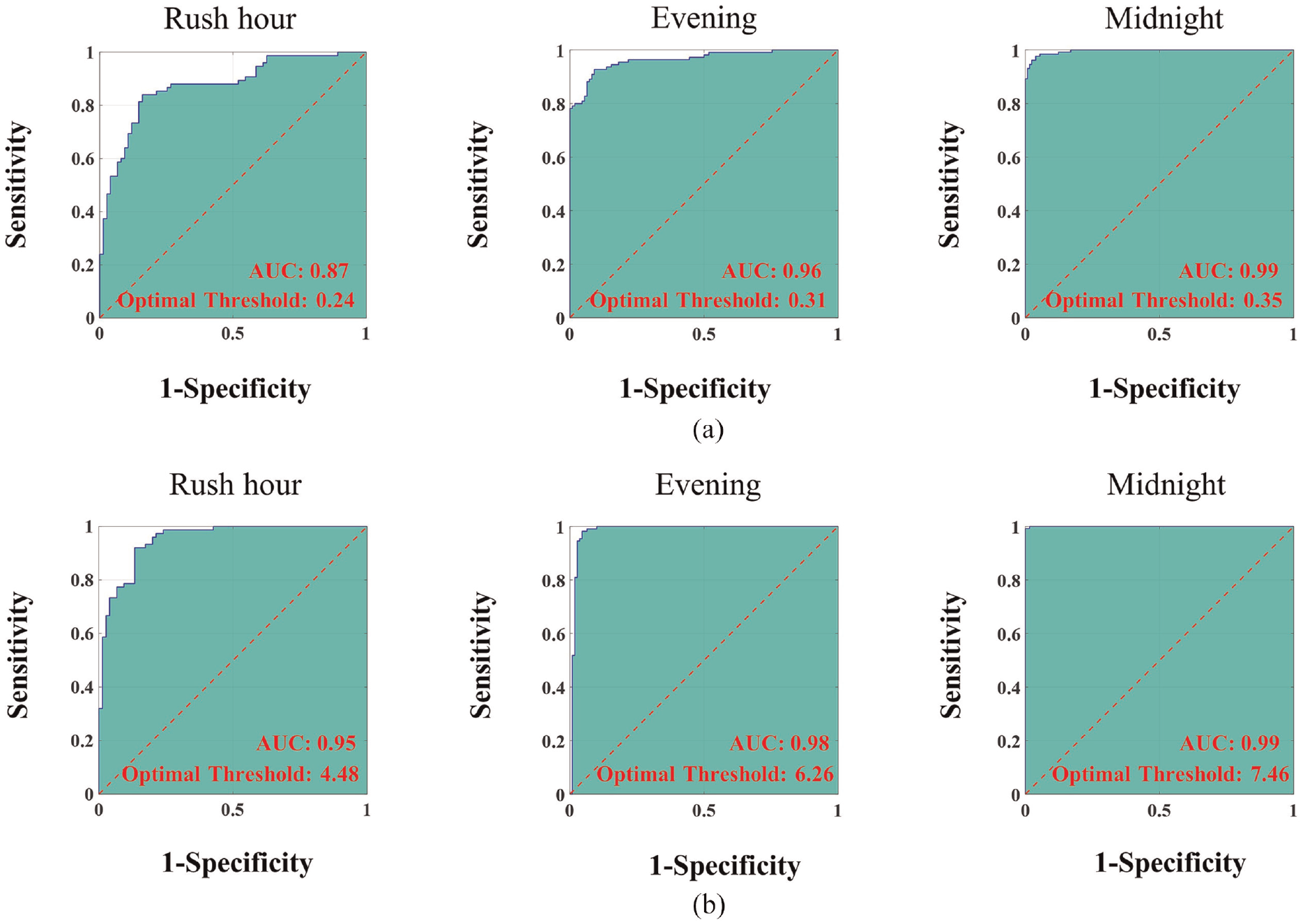
Results of classification performance using ROC curve and AUC at different times: (a) using only the impact signal and (b) using only the background noise signal.

In summary, the proposed algorithm requires a variable threshold value according to the noise environment. However, when the threshold values of MMSC_index and F _k were set to 0.25 and 5, respectively, impacts equal to or greater than 40 kN, which cause damage to buried pipelines, could be detected with high probability. In particular, the field applicability of the proposed algorithm and its performance were experimentally verified through performance evaluation and comparison with the actual background noise signal group.

Conclusion

In this study, we propose a new algorithm for identifying impact damage in the buried pipelines. In the field of SHM for buried pipelines, noise conditions can produce inaccurate results and are also difficult to control. Therefore, we focus on overcoming the challenges posed by noisy environments. The main highlights of this study are as follows:

Introduction of the KTF, a key component of the developed algorithm, which automatically improves the SNR of impact damage signals by observing the statistical characteristics of the impact damage signal.

By introducing MMSC_index and F _k as new decision indicators that utilize features in both the time and frequency domains, development and verification of essential anomaly detection algorithms for decision-making are conducted.

Successful field experiments on the large-scale in-service waterworks pipelines to verify the on-site applicability and performance of the proposed method in variable real-noise environments.

As a results, it was evaluated that the field applicability was higher than that of conventional methods, and the superiority of the proposed method was also verified through field experiments. Additionally, the performance of the proposed approach was quantitatively evaluated using the ROC curve. The method proposed in this study is expected to enable immediate response when the integrity of the buried pipelines is damaged due to external interference.

Footnotes

Declaration of conflicting interests

The authors declared no potential conflicts of interest with respect to the research, authorship, and/or publication of this article.

Funding

The author(s) disclosed receipt of the following financial support for the research, authorship, and/or publication of this article: This work was supported by Korea Environmental Industry and Technology Institute (MOE, 127587) and Korea Research Institute of Standards and Science (KRISS-GP2023-0011).

ORCID iDs

Sun-Ho Lee

Dong-Jin Yoon

References

Folkman

. Water main break rates in the USA and Canada: a comprehensive study. Report for the Mechanical and Aerospace Engineering. Report no. 174, 1 March 2018. Logan: Mechanical and Aerospace Engineering Faculty Publications, 2018.

Russo

Parisi

Augenti

, et al. Derivation of risk areas associated with high-pressure natural-gas pipelines explosions including effects on structural components. Chem Eng Trans 2014; 36: 289–294.

Chang

H-HR

. From gas explosions to earthquakes: case studies of disaster response in Taiwan. In: Masys

Lin

(eds.) Asia-Pacific security challenges: advanced sciences and technologies for security applications. Cham, Switzerland: Springer, 2018, pp.221–242.

Fentiman

Zabbey

. Environmental degradation and cultural erosion in Ogoniland: a case study of the oil spills in Bodo. Extr Ind Soc 2015; 2: 615–624.

Ali

Choi

. Risk prediction of sinkhole occurrence for different subsurface soil profiles due to leakage from underground sewer and water pipelines. Sustainability 2019; 12: 310.

Shiau

Chudal

Mahalingasivam

, et al. Pipeline burst-related ground stability in blowout condition. Transp Geotech 2021; 29: 100587.

Morgan

. Managing water main breaks: field guide. Denver: American Water Works Association, 2012.

Peng

Liu

. A surveillance system for urban buried pipeline subject to third-party threats based on fiber optic sensing and convolutional neural network. Struct Health Monit 2021; 20: 1704–1715.

Puust

Kapelan

Savic

, et al. A review of methods for leakage management in pipe networks. Urban Water J 2010; 7: 25–45.

10.

European Gas Incident Data Group. 7th EGIG-report 1970-2007 GAS PIPELINE INCIDENTS, Report for the European Gas Incident Data Group. Report no. EGIG 08.TV-B.0502, December 2008.

11.

Goodfellow

Lyons

, et al. UKOPA Pipeline Product Loss Incidents and Faults Report (1962–2019). Report for the United Kingdom Onshore Pipeline Operators’ Association. Report no. UKOPA/RP/21/001, July 2021. Ambergate: Pipeline Maintenance Centre.

12.

Brainard

Jr.

Leakage problems and the benefits off leak detection programs. J Am Water Works Assoc 1979; 71: 64–65.

13.

Cole

. Methods of leak detection: an overview. J Am Water Works Assoc 1979; 71: 73–75.

14.

Fuchs

Riehle

. Ten years of experience with leak detection by acoustic signal analysis. Appl Acoust 1991; 33: 1–19.

15.

Muggleton

Brennan

Linford

. Axisymmetric wave propagation in fluid-filled pipes: wavenumber measurements in in vacuo and buried pipes. J Sound Vib 2004; 270: 171–190.

16.

Hunaidi

Chu

. Acoustical characteristics of leak signals in plastic water distribution pipes. Appl Acoust 1999; 58: 235–254.

17.

Fuller

Fahy

. Characteristics of wave propagation and energy distributions in cylindrical elastic shells filled with fluid. J Sound Vib 1982; 81: 501–518.

18.

Muggleton

Yan

. Wavenumber prediction and measurement of axisymmetric waves in buried fluid-filled pipes: inclusion of shear coupling at a lubricated pipe/soil interface. J Sound Vib 2013; 332: 1216–1230.

19.

Lee

Y-S

Yoon

D-J

. Improved estimation of leak location of pipelines using frequency band variation. J Korean Soc Nondestruc Test 2014; 34: 44–52.

20.

Shin

S-M

Suh

J-H

J-S

, et al. Development of third-party damage monitoring system for natural gas pipeline. KSME Int J 2003; 17: 1423–1430.

21.

Park

C-S

Lee

S-H

Yoon

D-J

. Enhancing impact localization from fluid-pipe coupled vibration under noisy environment. Appl Sci 2021; 11: 4197.

22.

Kishawy

Gabbar

. Review of pipeline integrity management practices. Int J Press Vessels Pip 2010; 87: 373–380.

23.

Bao

Hao

. Vibration-based structural health monitoring of offshore pipelines: numerical and experimental study. Struct Control Health Monit 2013; 20: 769–788.

24.

Shinozuka

Lee

Kim

, et al. Lessons from two field tests on pipeline damage detection using acceleration measurement. In: Wu

(ed.) Nondestructive characterization for composite materials, aerospace engineering, civil infrastructure, and homeland security 2011. San Diego: SPIE, 2011, pp.668–677.

25.

Gao

Zhao

, et al. Fault diagnosis and location of the aero-engine hydraulic pipeline based on Kalman filter. Adv Mech Eng 2017; 9: 1687814017742811.

26.

Wang

, et al. Gas pipeline event classification based on one-dimensional convolutional neural network. Struct Health Monit 2022; 21: 826–834.

27.

Janapati

Kopsaftopoulos

, et al. Damage detection sensitivity characterization of acousto-ultrasound-based structural health monitoring techniques. Struct Health Monit 2016; 15: 143–161.

28.

Rytter

. Vibrational based inspection of civil engineering structures, PhD Thesis, Department of Building Technology and Structural Engineering, Aalborg University, Denmark, 1993.

29.

Müller

Janapati

Banerjee

, et al. On the performance quantification of active sensing SHM systems using model-assisted POD methods. In: Struct Health Monit 2011, pp.2417–2428.

30.

Tobias

. Acoustic-emission source location in two dimensions by an array of three sensors. Non Destruc Test 1976; 9: 9–12.

31.

Lee

Y-S

Yoon

D-J

Kang

, et al. Leak locating experiment for actual underground water supply pipelines with a novel locating system. Mod Phys Lett B 2008; 22: 1013–1018.

32.

Lee

Park

Yoon

. Experimental verification of impact damage detection in long range buried water supply pipeline. J Korean Soc Nondestruc Test 2020; 40: 241–250.

33.

Bjorklund

Ljung

. A review of time-delay estimation techniques. In: 42nd IEEE international conference on decision and vontrol (IEEE Cat No 03CH37475), Maui, HI, USA, 9–12 December2003, pp.2502–2507. New York, NY: IEEE.

34.

Chen

Huang

Benesty

. Time delay estimation. In: Huang

Benesty

(eds.) Audio signal processing for next-generation multimedia communication systems. Boston, MA: Springer, 2004, pp.197–227.

35.

Hafezi

Mirhosseini

. Application of cross-correlation in pipe condition assessment and leak detection; using transient pressure and acoustic waves. Resour Environ 2015; 5: 159–166.

36.

Gao

Brennan

Liu

, et al. Improving the shape of the cross-correlation function for leak detection in a plastic water distribution pipe using acoustic signals. Appl Acoust 2017; 127: 24–33.

37.

Papastavrou

G-N

Kousiopoulos

G-P

Kampelopoulos

, et al. Leak detection algorithm for pipelines in noisy environments. In: 2020 IEEE 20th mediterranean electrotechnical conference (MELECON), Palermo, Italy, 16–18 June 2020, pp.159–164. New York: NY: IEEE.

38.

Ionel

. The majority principle in TDOA estimation. In: 2010 8th international conference on communications, Bucharest, Romania, 10–12 June 2010, pp.21–24. New York, NY: IEEE.

39.

Lee

Y-S

. Effects of windowing filters in leak locating for buried water-filled cast iron pipes. J Mech Sci Technol 2009; 23: 401–408.

40.

Roth

. Effective measurements using digital signal analysis. IEEE Spectr 1971; 8: 62–70.

41.

Carter

Nuttall

Cable

. The smoothed coherence transform. Proc IEEE 1973; 61: 1497–1498.

42.

Hannan

Thomson

. Estimating group delay. Biometrika 1973; 60: 241–253.

43.

Streit

Willett

. Detection of random transient signals via hyperparameter estimation. IEEE Trans Signal Process 1999; 47: 1823–1834.

44.

Digulescu

Bernard

Lungu

, et al. Transient signal characterization using multi-lag phase space analysis. In: 2015 IEEE international conference on microwaves, communications, antennas and electronic systems (COMCAS), Tel Aviv, Israel, 2–4 November 2015, pp.1–5. New York: NY: IEEE.

45.

Hinich

. Detecting a transient signal by bispectral analysis. IEEE Trans Acoust Speech Signal Process 1990; 38: 1277–1283.

46.

Helstrom

. The resolution of signals in white, Gaussian noise. Proc IRE 1955; 43: 1111–1118.

47.

Rahmani-Andebili

(ed.). Problems: analysis of transient response. In: Feedback control systems analysis and design. Cham: Springer, 2022, pp.39–43.

48.

Scharf

Demeure

. Statistical signal processing: detection, estimation, and time series analysis. Hoboken, NJ: Prentice Hall, 1991.

49.

Mansour

Jutten

. What should we say about the kurtosis? IEEE Signal Process Lett 1999; 6: 321–322.

50.

Dwyer

. A technique for improving detection and estimation of signals contaminated by under ice noise. J Acoust Soc Am 1983; 74: 124–130.

51.

Dwyer

. Use of the kurtosis statistic in the frequency domain as an aid in detecting random signals. IEEE J Ocean Eng 1984; 9: 85–92.

52.

Pearson

. Das fehlergesetz und seine verallgemeiner-ungen durch fechner und pearson: a rejoinder. Biometrika 1905; 4: 169–212.

53.

Westfall

. Kurtosis as peakedness, 1905–2014: RIP. Am Stat 2014; 68: 191–195.

54.

Darlington

. Is kurtosis really “peakedness?” Am Stat 1970; 24: 19–22.

55.

Randall

. Frequency analysis. Naerum, Denmark: Bruel & Kjaer, 1987.

56.

McClish

. Analyzing a portion of the ROC curve. Med Decis Making 1989; 9: 190–195.

57.

Bradley

. The use of the area under the ROC curve in the evaluation of machine learning algorithms. Pattern Recognit 1997; 30: 1145–1159.