
Abstract
Wind turbines usually operate in mountainous, offshore and other field environments. As the wind speed is constantly changing, the gearboxes of wind turbines operate under variable operating conditions, resulting in a non-stationery and time-varying signal characteristic. For existing time–frequency analysis (TFA) methods, they undergo low time–frequency energy concentration as well as noise interference during the fault feature extraction. IMFogram, a recently proposed time–frequency representation (TFR) method, calculates local frequency and amplitude information of signals based on fast iterative filtering (FIF). Moreover, it is able to remove uncertainty on the time–frequency plane, allowing a long enough time window to reduce the local boundary effects associated with the signal decomposition methods. Therefore, it has potential advantages for TFA. However, the actual performance of IMFogram calculation largely depends on the decomposition effect provided by FIF and the selection of model parameters. With the purpose of obtaining a more distinct and focused TFR of the wind turbine vibration signal, a novel TFA method, namely Adaptive IMFogram (AIMFogram), is proposed in this paper. Firstly, a range of intrinsic mode functions (IMFs) are gained after the decomposition of vibration signals using an improved variational nonlinear chirp mode decomposition, which is treated as the input to AIMFogram to solve the unsatisfied result by traditional FIF under strong noise. Secondly, Renyi entropy-based particle swarm optimization is conducted to perform adaptive parameter optimization of the AIMFogram. Later, using the optimal parameter, the proposed AIMFogram achieves a high-resolution TFR of complex multi-component vibration signals. To verify whether the proposed AIMFogram is effective or not, the method was successfully employed to the fault diagnosis of the rolling bearing in an experimental bench and the gearbox in a 850-kW wind turbine.
Keywords
Introduction
With quick depletion of global energy resources, more and more countries are turning to wind energy as their main source of renewable energy. According to statistics, global wind power generation has been growing at an average annual rate of 15.9% since 2009, and the Global Wind Energy Report 2023 states that new grid-connected capacity of global wind power is expected to reach 680 GW in the next 5 years.1,2 However, as wind turbines often stand in remote mountainous and coastal areas, they are subjected to high winds and other impacts from the outside environment, resulting in a dramatic increase in the failure rate of turbine components under severe operating conditions. The occurrence of a fault will have a significant impact on the normal function of the equipment which is particularly critical for expensive large-scale wind turbines since a small error could also lead to substantial economic losses. Therefore, it has great engineering importance to realize fault feature recognition of wind turbine gearbox.3,4
The operating conditions of planetary gearboxes in wind turbine drive trains usually vary due to the changing wind speed, resulting in significant non-stationary feature of vibration signals. For these signals, the spectral characteristics are time-varying. Traditional analysis methods in time domain or frequency domain alone cannot fully describe the non-stationary characteristics, while time–frequency analysis (TFA) provides information on the variation of signal spectrum with time, proving itself to be an effective tool for non-stationary signal processing.5,6
In the course of past research, Short-time Fourier Transform (STFT) and the Continuous Wavelet Transform are frequently employed for TFA. However, due to the limitations imposed by the Heisenberg uncertainty principle, it is difficult for signals to simultaneously achieve optimal resolution in both time and frequency domains.7,8 These disadvantages of the traditional TFA methods reduce the sensitivity of the diagnostic system to less obvious faults, for instance, early weak failures and faults under noisy environments. 9 To improve TFA methods’ ability of detecting failures under complicated environments, a number of advanced methods have been presented over the past years. Daubechies et al. 10 proposes the Synchrosqueezing Transform (SST), which utilizes a Synchrosqueezing algorithm to compress time–frequency coefficients to their respective instantaneous frequency locations. This method improves the resolution of the time–frequency plane by concentrating the time–frequency curves. Empirical Mode Decomposition 11 (EMD) is a signal decomposition method that is adaptive in nature. It decomposes a signal into multiple Intrinsic Mode Functions (IMFs) that represent its local characteristics of the signal based on its time scale. The IMFs containing fault components exhibit more pronounced transient features. 12 Hilbert-Huang Transform 13 (HHT) is based on the EMD and then applies the Hilbert transform to compute the analytic signal associated with each IMF, thereby obtaining the instantaneous frequency curve in the time–frequency domain. However, EMD suffers from modal confusion, endpoint effects and difficult determination for stopping conditions.14,15 For the sake of overcoming these drawbacks, variational mode decomposition (VMD) decomposes the signal into a variable division mode, which essentially employs multiple sets of adaptive Wiener filters to realize adaptive segmentation. 16 Comparing with the EMD, VMD provides greater noise robustness and achieves weaker endpoint effects. 17 However, there exists some difficulties in the decomposition when choosing the appropriate hyperparameters, including the number of decomposition patterns, the initial center frequency and the balance parameters. 18 In addition, VMD is limited to processing signals in narrowband modes and does not work well for the analytical processing of modulated signals in broadband modes, especially those containing crossover modes. Hence, variational nonlinear chirp mode decomposition (VNCMD) is designed to convert broadband signals into narrowband signals using demodulation techniques. 19 Moreover, it is able to extract all signal patterns simultaneously. Nevertheless, similar to VMD, it suffers from the same problem of requiring a priori knowledge to determine parameters such as the initial center frequency.20,21
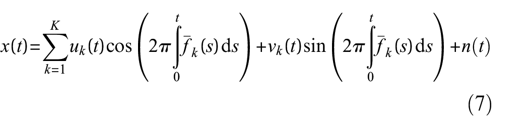
Recently, Antonio et al. proposed a TFA method called IMFogram.22,23 The method first calculates the decomposition of the signal by fast iterative filtering (FIF), and then analyses each decomposed IMF using IMFogram. It identifies both local frequency and local amplitude information for each IMF at the same time and ultimately produces a time–frequency representation (TFR) with accurate resolution. Although IMFogram provides a clearer and more focused TFR, it still has some shortcomings. Firstly, FIF is a fast implementation of Iterative Filtering (IF) on the basis of the Fast Fourier Transform (FFT) framework and is a moving average obtained by means of a double convolution filter. However, this filter is not smooth enough and its IMFs fluctuates spuriously under the disturbance of strong oscillations. Secondly, the practical effectiveness of IMFogram for TFA of multi-component signals is mainly influenced by the choice of several parameters, such as the number of instantaneous frequencies and the length of the time sliding window.
Therefore, a novel TFA method, called adaptive IMFogram (AIMFogram), is put forward in this paper and is applied to achieve high-resolution TFR of vibration signals of wind turbines. AIMFogram is put forward based on the theoretical framework of the existing IMFogram. Firstly, VNCMD is used to replace the FIF as the input to the AIMFgram to avoid interference from other frequency band oscillations. However, since VNCMD relies on the initial center frequency setting, this paper obtains the initial center frequency of the signal by means of a popular multi-ridge detection (MRD) algorithm.23,24 Secondly, particle swarm algorithm (PSO) is chosen as the parameter adaptive optimization method for the AIMFogram in this paper. Renyi entropy is also employed as the fitness function to gain the optimal position of the particles, and finally the optimal combination of parameters is selected for the AIMFogram, namely, the number of drawn IMFs and the sliding time window length.
The remaining sections of this paper are organized as follows: in Section “Theoretical descriptions,” the basic theory of IMFogram and VNCMD is introduced, followed by a detailed theoretical description of AIMFogram, and later the process steps of the wind turbine fault diagnosis are described. In Section “Analogue signal simulation analysis,” analogue signal simulation analysis with time-varying features will be employed to verify the superiority of the proposed AIMFogram. In Section “Experimental data analysis,” the proposed method will be applied for vibration signal analysis on a test rig and an 850-kW wind turbine gearbox with rolling bearing fault. These measurement data will further demonstrate the effectiveness of the proposed AIMFogram. Finally, Section “Conclusion” concludes the paper.
Theoretical descriptions
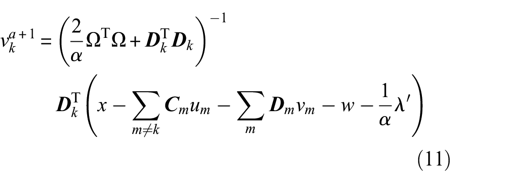
IMFogram
IMFogram is an analogue of a spectrogram which allows fast calculations based on the decomposition results and identification for both local frequency and amplitude information of the signal. Antonio decomposes the signal in the literature 22 using FIF, which is an IF based on a fast implementation of the FFT. The basic idea is to decompose a non-linear and non-smooth signal into IMFs by means of a double convolution filter. Next, a stopping criterion is introduced to ensure the termination of the algorithm. Finally, each IMF is analyzed from a time–frequency perspective to obtain a TFR of the IMFogram.
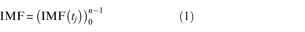
First, the IMF is defined as:
where
Arrange

where
Let the zero crossings of
The IA and IF of the final IMF at
Define the average matrix
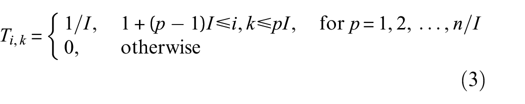
where
In the next step, set

Rewrite the parameters based on the above theoretical derivation, the IMFogram matrix
where
The IMFogram produces TFR results from time domain, local period and local amplitude information, and makes its TFR results more localized by adding windows to the signal. If watching closely, one can see that the TFR results look like they are made up of many rectangular windows. Thus, it is possible to represent the decomposed results accurately on the time–frequency plane.
Proposed AIMFogram algorithm
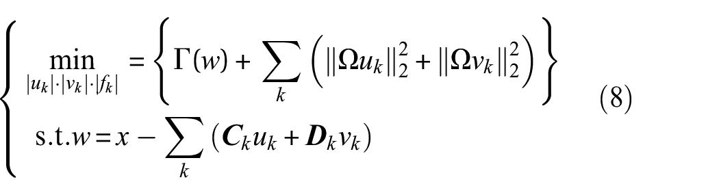
The actual effectiveness of the original IMFogram depends on the results of the FIF decomposition, but two problems still exist in the vibration signal decomposition. Firstly, to make the result of the decomposition more reflective of the local signal characteristics, the filter function must be of finite length. However, the waveform of a filter function with finite length is not smooth enough in general. Secondly, under the influence of noise, there will still be a noisy component in the multiple IMF components of the FIF decomposition, which will directly lead to a time–frequency curve of noise in the time–frequency diagram obtained by the IMFogram. In addition, the IMFogram-calculated results of the TFR depend on the correct selection of parameters. As a result, this paper will improve on the IMFogram and propose an adaptive IMFogram (AIMFogram). At first, we replace FIF with VNCMD, which means using a demodulation technique to convert a broadband FM signal into a narrowband signal and then decomposing the signal into multiple nonlinear chirp mode components by means of a variational model that is more suitable for the vibration signal analysis under speed changing conditions. However, VNCMD requires the setting of an initial center frequency (ICF), which demands a priori knowledge. Therefore, this paper proposes to use MRD to extract the coarser time–frequency distribution ridges of the STFT as the ICF.24,25 Then, by introducing a PSO algorithm and combining it with the Renyi entropy model, the AIMFogram is made to achieve adaptive optimization of the parameters.
Improved VNCMD
In practical scenarios, signals often consist of multiple nonlinear frequency-modulated modes accompanied by Gaussian white noise. The mathematical model
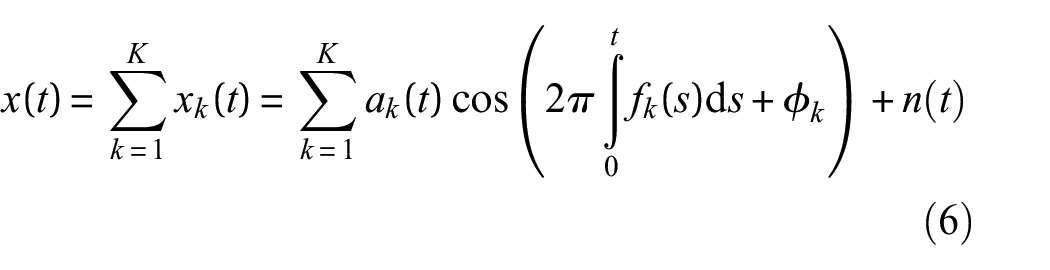
where
where
Since the data analyzed are usually sampled in discrete form, when the sampling interval is
where
To address the issue in Equation (8), the Lagrangian multiplier
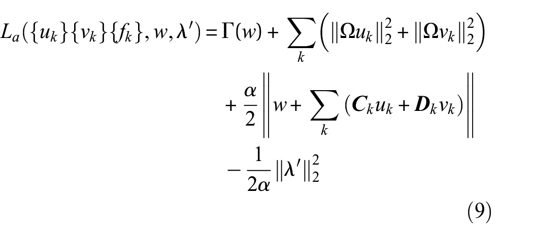
where
Further, alternating direction method of multipliers algorithm is used for instantaneous frequency optimization as well as modal component solution. The specific steps are followed below:
Step 1, update both demodulation signals:
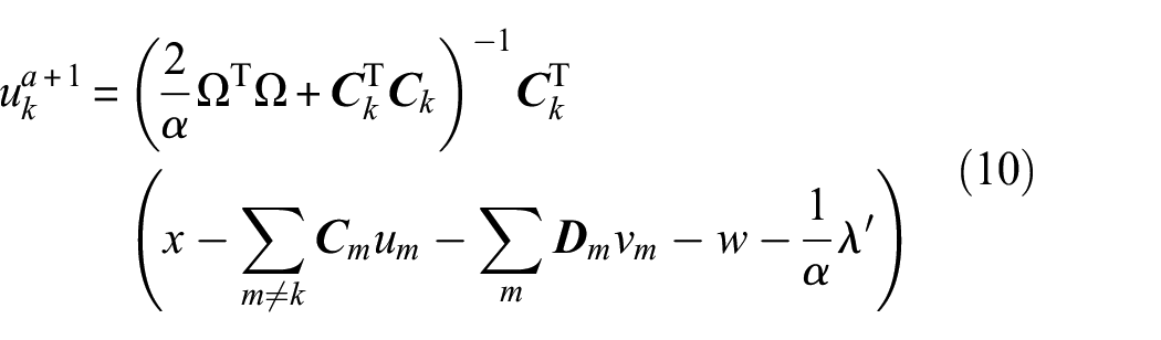
Step 2, the instantaneous frequency
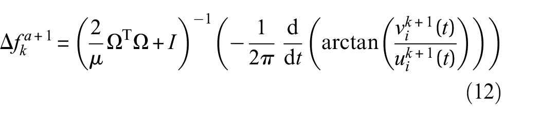

where
Step 3, update and reconfigure the signal

Due to the limitations of the algorithm, VNCMD requires an initial IF that is artificially preset and the estimated frequency band of the pattern depends on the initial IF. For the sake of solving the problem of initial IF for each mode component, a popular multi-ridge detection algorithm of MRD24,25 is proposed to perform initial IF extraction on the time–frequency results of STFT. By predefining the number of modes K, the calculation formula for this algorithm is as follows:
where
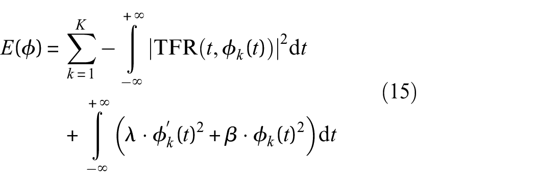
Adaptive optimization of parameters for IMFogram
If IMFogram is to gain a TFR of the energy concentration of vibration signal, it depends primarily on the number
Each particle in the PSO has two properties: velocity and position. The two properties of particle
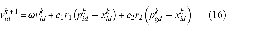

In the Equation, k represents the iteration number; i represents the particle’s index; d represents the dimensionality of the particle;
With the purpose of finding the best position for the particle, an adaptation function is required to be given. Therefore, calculate the fitness function value one time after every iteration and update the position and velocity of particle by comparing the function values. The inertia weights of the PSO only guarantee the general direction of the swarm search but cannot precisely control each iteration of the algorithm. The Renyi entropy, as an extension of the information entropy, reflects the features of the signal in terms of its time–frequency distribution.
28
Compared to information entropy, Renyi entropy is more sensitive to the subtle signal changes, making it easier to identify small changes in the signal. Therefore, this paper optimizes the PSO algorithm based on the Renyi entropy model, and obtains characteristics information of the particle swarm in the search process. The inertia weights of each iteration are dynamically adjusted based on the entropy difference, so as to gain the optimal parameter combination for the IMFogram algorithm, that is, the number
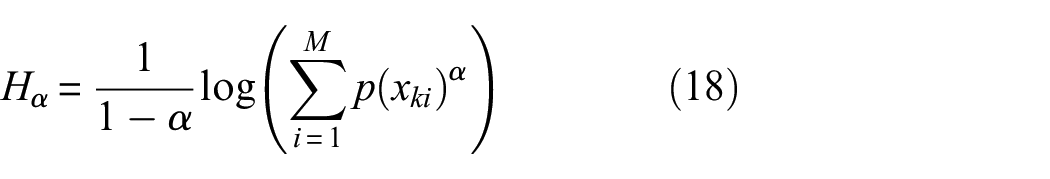
Renyi entropy is calculated as
where
The entropy value is not always in a straight line down, there can be an increase. The entropy difference represents the absolute magnitude of the difference between the minimum entropy value and the entropy value after the latest iteration of optimization search. The formula is as follows:

The specific steps of the parametric adaptive optimization IMFogram algorithm are described below:
(1) Initialize the optimization parameters
(2) Initialize the PSO parameters and set the Renyi entropy to the fitness function.
(3) Aiming at every particle, compare its current fitness with the fitness at its best position encountered so far. If the fitness improves, update
(4) Compare the best fitness of each particle with the fitness at the best position encountered by the swarm. If the former is better, update the best minimum of individual and population history
(5) Adjust the speed and position of the particle and repeat steps (1)–(4). If the maximum number of iterations is reached or the entropy difference becomes zero, the particle search ends and optimum position of the particle is output.
(6) The result of experiencing the best positioned particle is used as the global optimal weight, that is, the value after decoding of the best position encountered by the swarm, which is used as the structural parameter of the IMFogram.
Procedure of the proposed AIMFogram
Under variable speed conditions, the obtained fault characteristic frequencies after time–frequency transformation are time-varying, and traditional fault diagnosis methods have difficulty in identifying their changing instantaneous frequency. Therefore, based on the existing IMFogram theoretical framework, this paper proposes an enhanced variational nonlinear chirp mode decomposition, which achieves the acquisition of the IMF after signal decomposition without prior knowledge. A PSO algorithm based on Renyi entropy is then used to gain the best parameter combination for IMFogram, thus achieving the optimal TFR of IMFogram. The proposed fault diagnosis method follows the procedure below:
(1) First, use an improved VNCMD for the mode decomposition of the wind turbine vibration signal to obtain a number of component IMFs.
(2) Then, using the proposed AIMFogram method, an optimal TFR of the multi-component signal of wind turbine vibration is achieved by determining the parameter combination through PSO and Renyi entropy.
(3) Finally, by calculating the fault characteristic frequencies and extracting the relevant instantaneous frequency curves from the time–frequency plots, the identification of rolling bearing fault types in variable speed operating conditions of the wind turbine is achieved. The flow chart of the proposed AIMFogram applied to fault diagnosis is shown as the Figure 1 below.
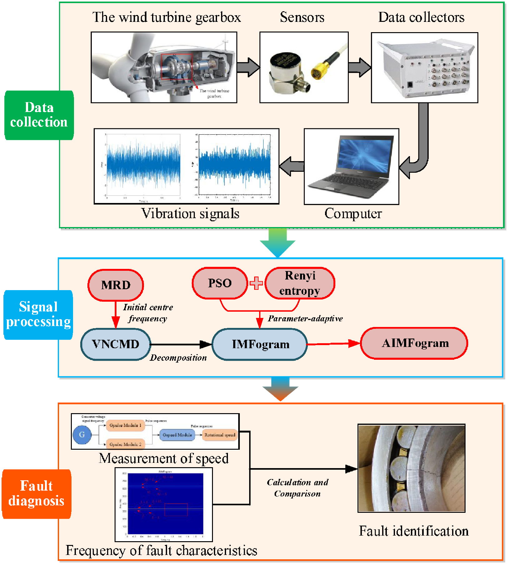
General diagram for fault diagnosis using AIMFogram.
Analogue signal simulation analysis
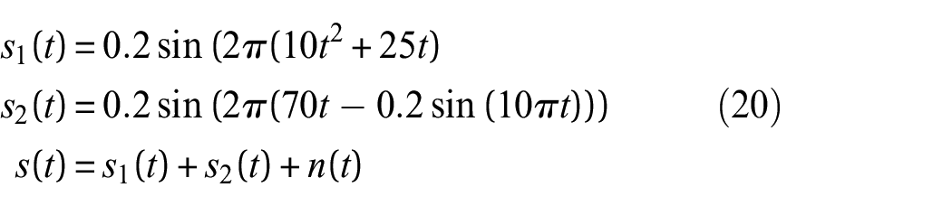
To validate the advantages of the AIMFogram algorithm, a set of multivariate simulated signals with frequency variations over time are utilized for analysis. The simulated signal is configured as follows:
where
The time domain waveform of the analogue signal is drawn in Figure 2(a) and the corresponding frequency spectrum is plotted in Figure 2(b). From the spectrum, the signal components at 25–45 and
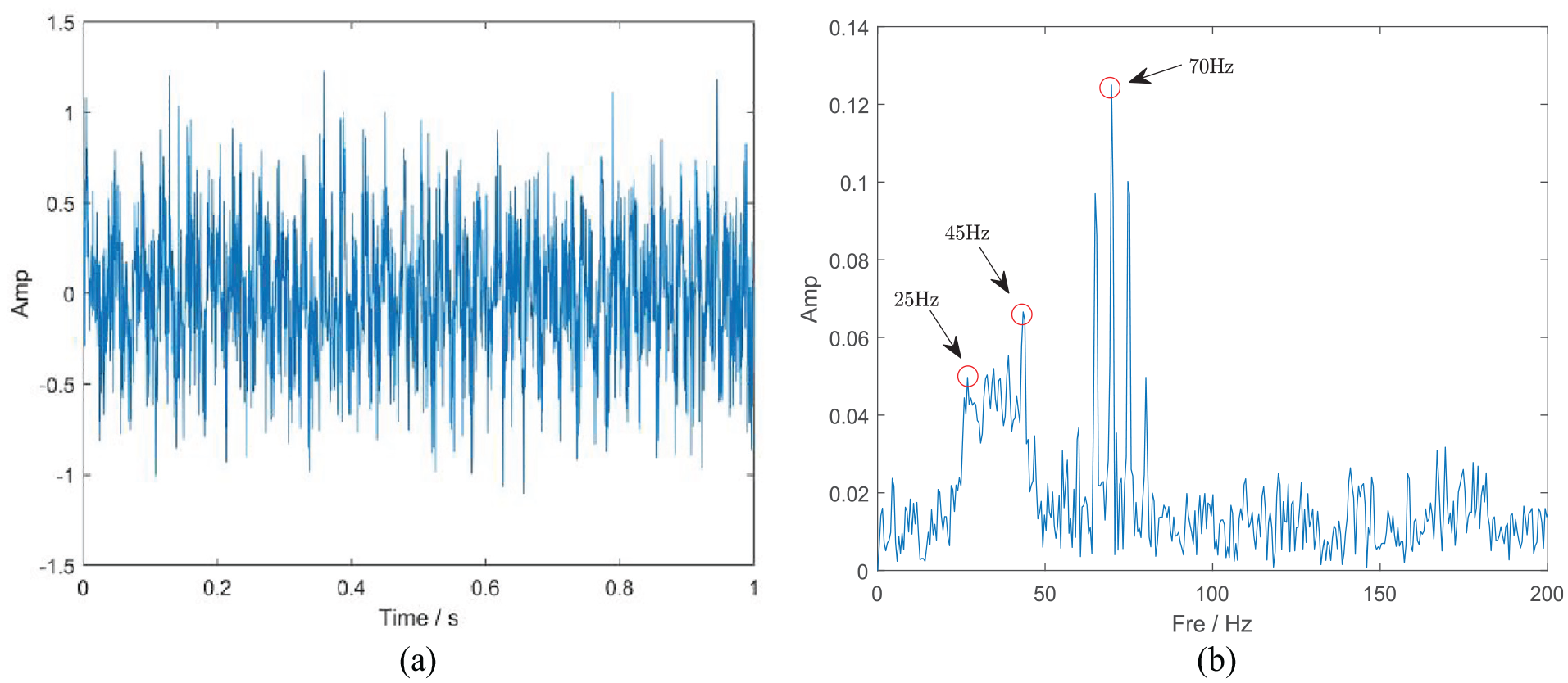
Time domain diagram and frequency spectrum of analogue signal. (a) Time domain diagram of analogue signal and (b) frequency spectrum of analogue signal.
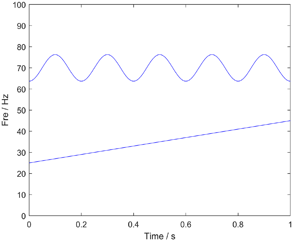
Ideal IF curve for analogue signal.
For the signal as STFT, the window function is chosen as Gaussian window function with a window width of 300, and the computations displayed in Figure 4(a). Obviously, the STFT results are blurred at time–frequency plane. The signal calculation results using SST are expressed as Figure 4(c), where to some extent energy in the time–frequency plane is concentrated, but the IF curve still suffers from energy divergence as can be seen from the local plot in Figure 4(d). Subsequently, Figure 4(e) and (f) demonstrate the TFR and local plots of the IMFogram by FIF after its decomposition. It can be found that energy dispersion in the time–frequency plane has been solved, but due to signal modulation and the influence of noise, the result obtained after FIF decomposition has a large deviation from the ideal IF curve, and there still presents noise. Figure 4(g) and (h) plot the TFR of the above signals using AIMFogram. The initial population size of the particle swarm is 40, the inertia weight
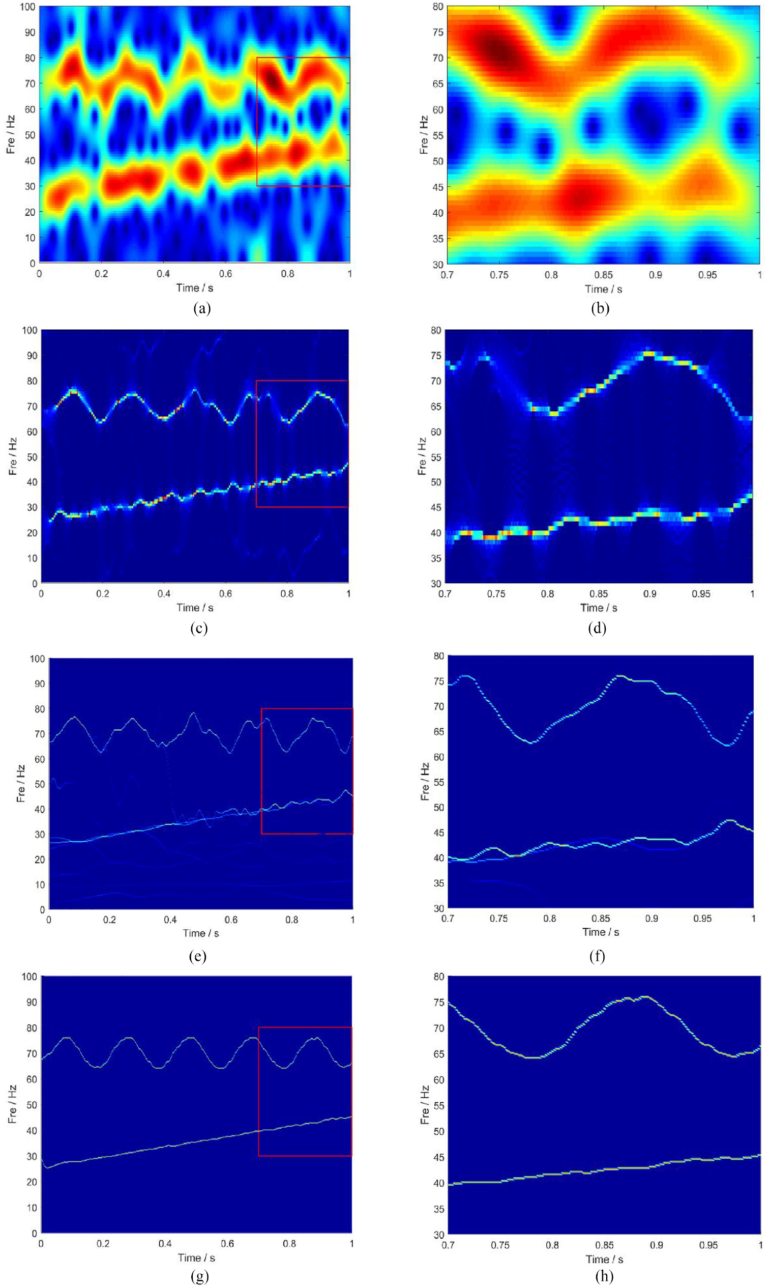
TFR of the simulated signal by different methods. (a) Result provided by STFT, (b) partial view of STFT result, (c) result provided by SST, (d) partial view of SST result, (e) result provided by IMFogram, (f) partial view of IMFogram result, (g) result provided by AIMFogram, and (h) partial view of AIMFogram result.
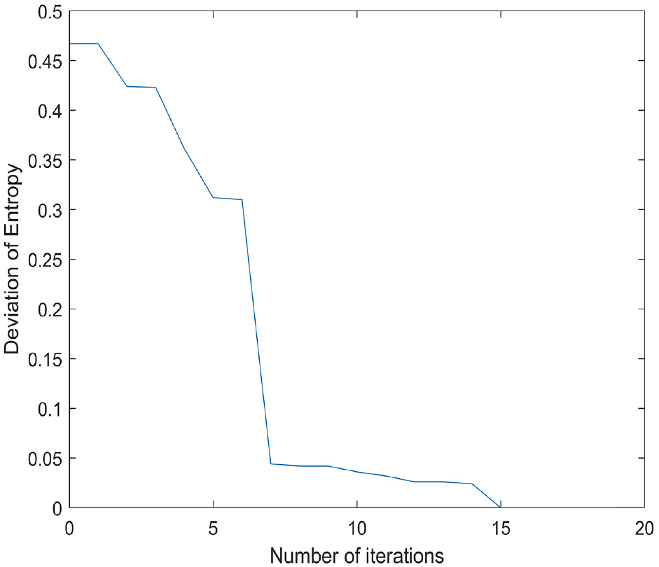
Variation of entropy difference with the number of iterations.
To demonstrate the superiority of the VNCMD method over the FIF algorithm in signal decomposition, this study conducts an analysis using two performance metrics: correlation coefficient and mean square error (MSE). The correlation coefficient is a metric used to assess the correlation between the decomposed synthesized signal and the original noise-free signal. The value of correlation coefficient closer to 1 always indicates a stronger correlation between the two signals. Commonly, the smaller the MSE value is, the stronger the multi-component signal decomposition ability of the employed algorithm is. Therefore, we investigate the performance of function indicators under different noise environments, as shown in Figure 6. In Figure 6(a), VNCMD clearly outperforms FIF. In Figure 6(b), for relatively high SNR values, VNCMD and FIF display similar MSE values, but as the SNR drops below 10 dB, the MSE of FIF increases dramatically. Therefore, VNCMD exhibits superior decomposition performance compared to FIF.
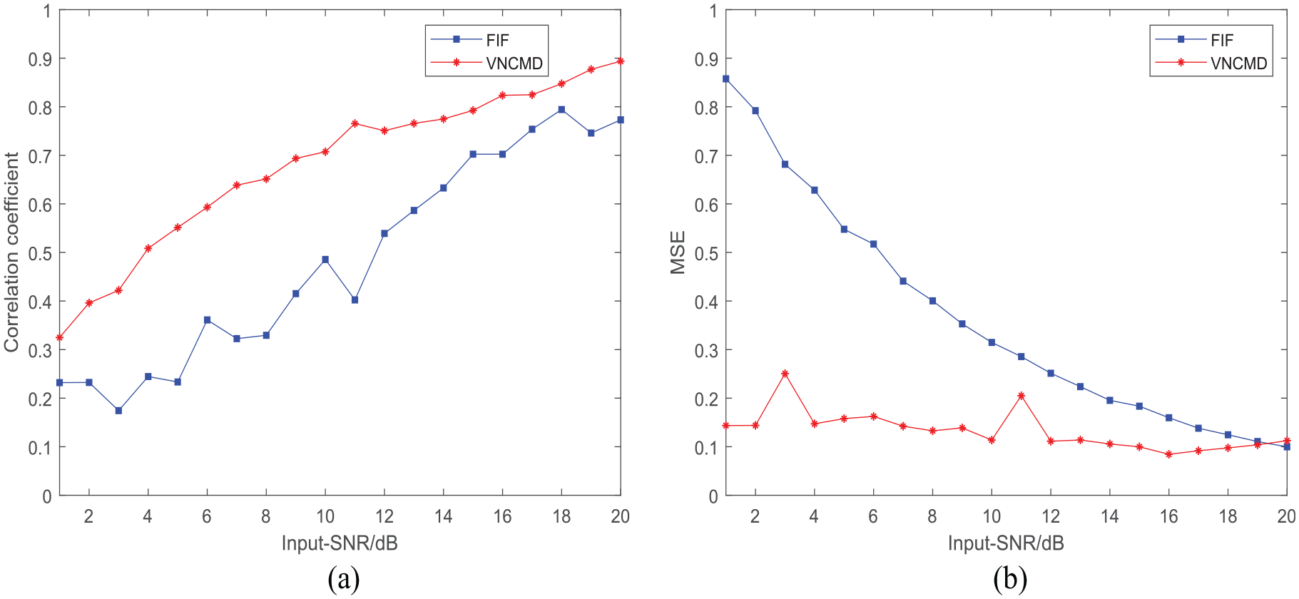
The variation of the performance metrics with SNR input. (a) Correlation coefficient, and (b) MSE.
To assess the performance of the aforementioned methods in terms of TFR, this study quantitatively analyzes the concentration of energy in the IF curves of different TFA methods using Renyi entropy values. 29 Commonly, the lower Renyi entropy value indicates a more concentrated TFR. Figure 7 shows the Renyi entropy values for four different methods in different noise scenarios. As can be seen from the Figure 7, the researched AIMFogram has the lowest Renyi entropy, showing that it comprehensively outperformed the other methods in TFA.
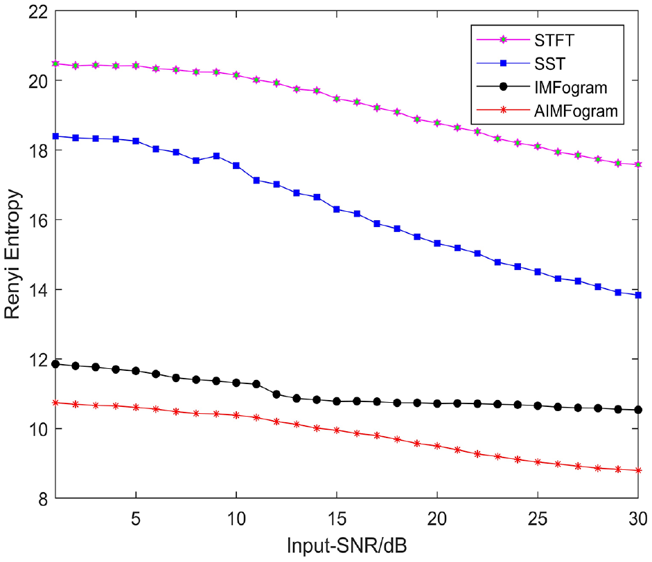
Renyi entropy for different methods with different noise.
Experimental data analysis
Application to rolling bearings with outer ring failures on test bench
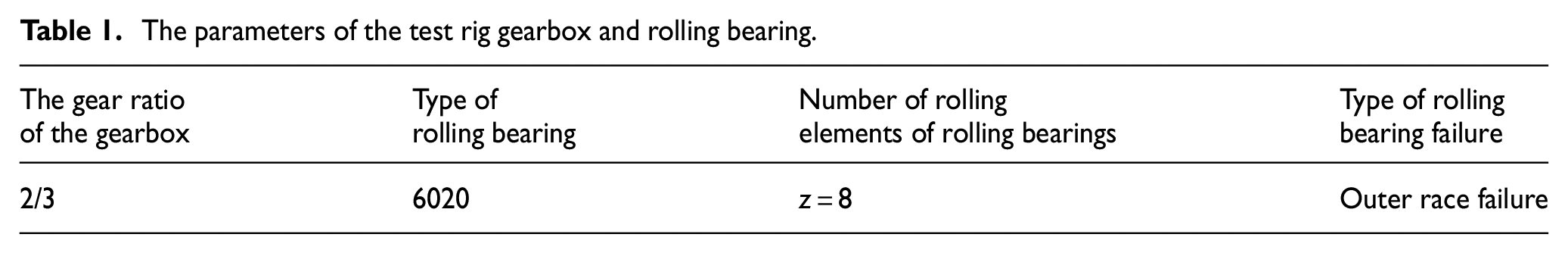
To further verify whether the proposed method in practical applications is effective or not, experimental analysis was carried out using test bench data. A physical diagram and a sketch of the structure of the test rig is shown in Figure 8. During the experiment, the motor gradually accelerated from a stationary state to 1920 rpm in 10 s. The vibration acceleration sensor was radially placed on the external bearing housing for measurement. We collected the acceleration process and selected the final 1.6 s of the acceleration period for analysis, with a sampling frequency of 2560 Hz. Table 1 lists the parameters of the test bench and the model of the faulty rolling bearing in detail. The vibration signal and its frequency spectrum acquired from the test bench are shown in Figure 8.
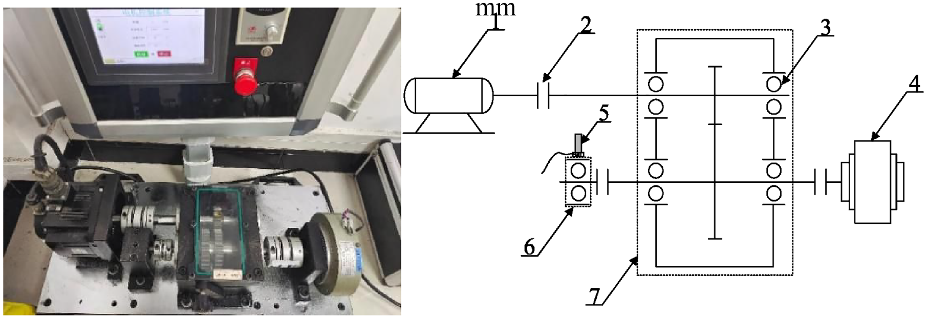
Physical drawing and structural sketch of the experimental bench. 1- Servo motors, 2- Couplings, 3- Bearing seat, 4- Magnetic powder brake, 5- PCB acceleration sensors, 6- External bearing seat, 7- Gearboxes.
The parameters of the test rig gearbox and rolling bearing.
The feature frequency of the bearing failure could not be clearly determined in the spectrum of Figure 9(b); thus the results gained by STFT of the acquired signal are demonstrated in Figure 10(a) and Fig. 10 (b) shows its local enlargement. From this it is clear that due to the inevitable noise and other interference factors in actual measurement process, the time–frequency energy ridge clearly diverges in its local magnification, and its instantaneous frequency cannot be accurately obtained. The analysis results provided by SST are presented in Figure 10(c), with its local enlargement in Figure 10(d), from which the components in the signal can be seen apparently. However, the IF trajectory still exhibits a slight energy divergence. The IMFogram analysis results are shown in Figure 10(e), from which it can be found that the interference of rotating frequency and noise lead to deviations in the components obtained after FIF decomposition, such as triplets of the fault characteristic frequency. There is also information of noise, which causes interference in the next fault diagnosis. Figure 10(f) shows its local magnification; it is obvious that the time–frequency ridge energy is more concentrated compared to those of STFT and SST, but other components exist.
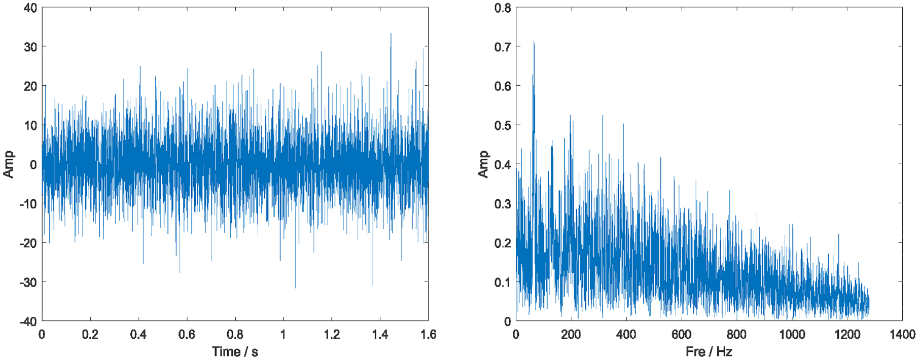
Vibration signal and its frequency spectrum from the test bench. (a) Vibration signal from the test bench and (b) frequency spectrum of the vibration signal.
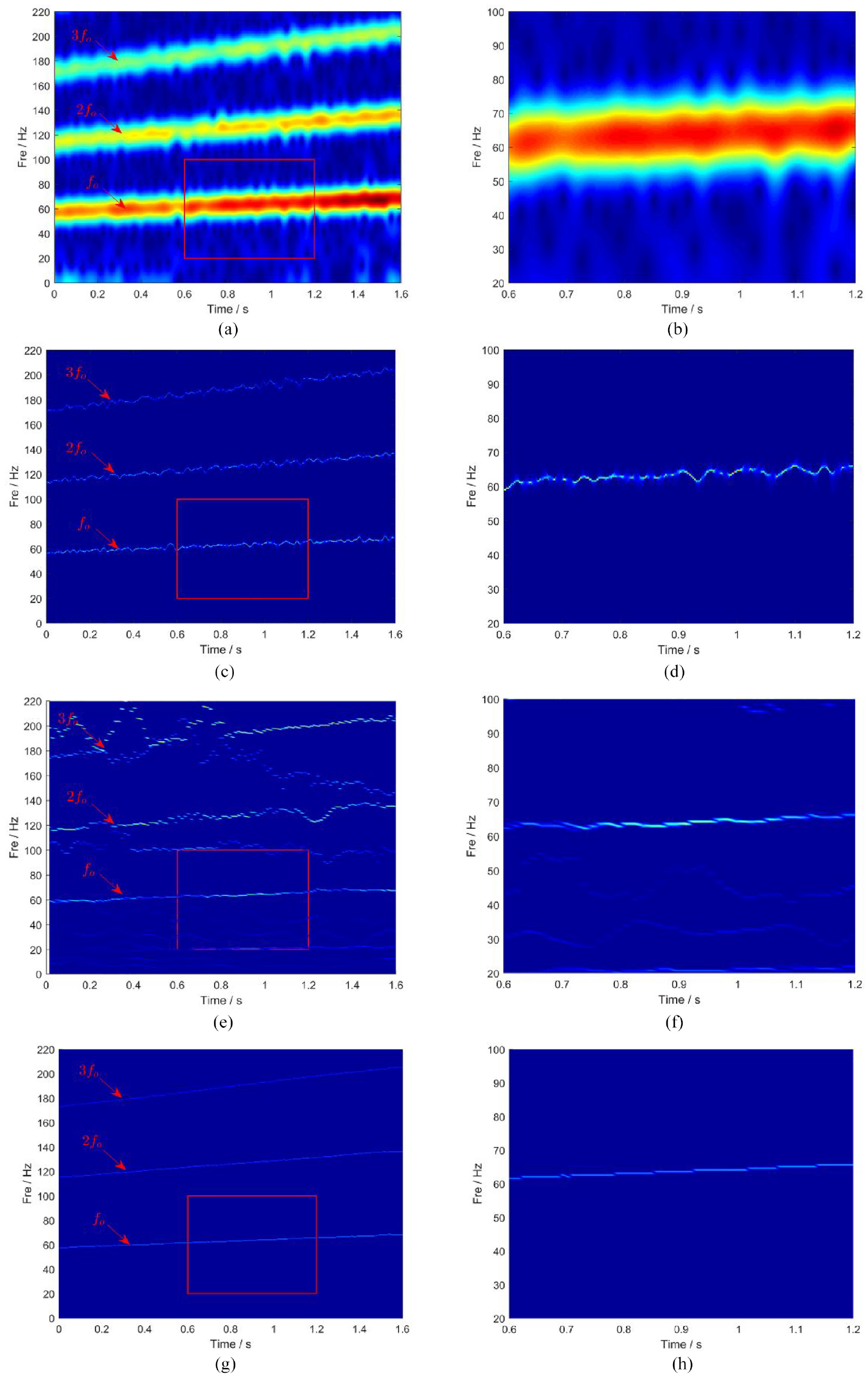
TFR of the vibration signal for four different methods. (a) Result provided by STFT, (b) partial map of STFT result, (c) result provided by SST, (d) partial map of SST result, (e) result provided by IMFogram, (f) partial map of IMFogram result, (g) result provided by AIMFogram, and (h) partial map of AIMFogram result.
The TFA results generated by AIMFogram are presented in Figure 10(g) and (h). The initial population size of the particle swarm is 60, the inertia weight
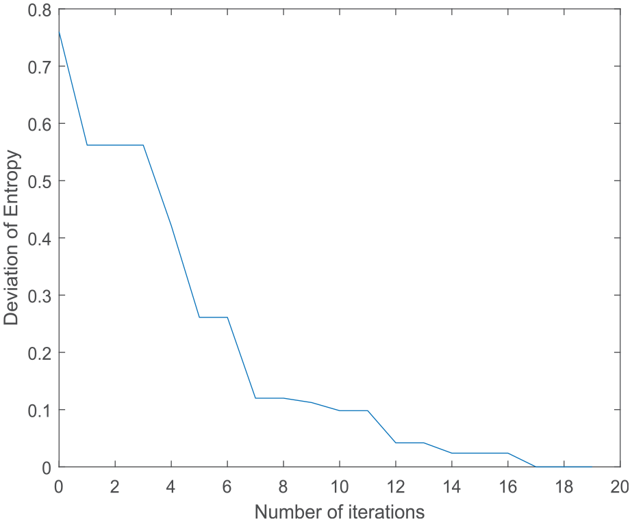
Variation of entropy difference with the number of iterations.
Theoretically, the fault characteristic frequencies of the rolling bearing, namely, the ball passing frequency of outer race
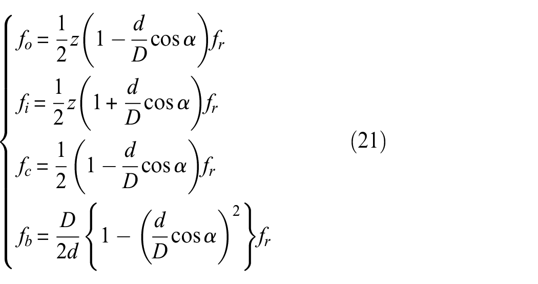
where
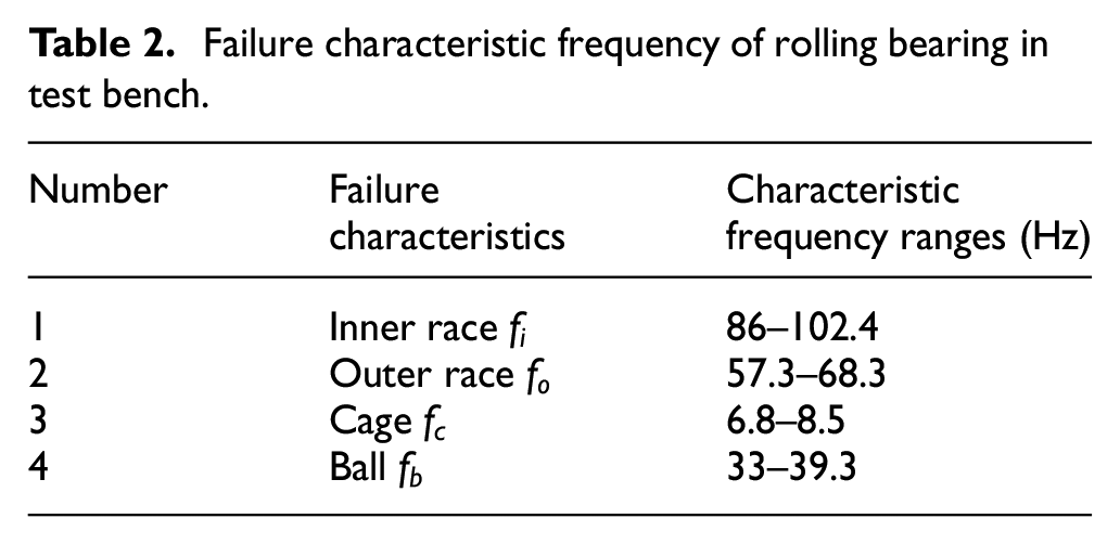
According to the rolling bearing of test bench type 6206 and the fluctuation range of among 17.9–21.3 Hz, we used the rolling bearing failure characteristic frequency formulae (21) to calculate the failure characteristic frequency of the inner race
Failure characteristic frequency of rolling bearing in test bench.
Application to wind turbine gearbox fault identification
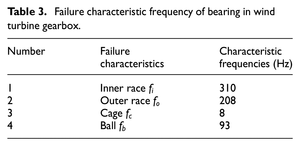
The actual measured vibration signal is sourced from an 850-kW wind turbine unit located at a wind farm operated by Goldwind Sci & Tech Co., Ltd. (Urumqi, China). It was collected from the sensor measuring point of the high-speed shaft front bearing of the gearbox during the operation of a specific wind turbine. This dataset is utilized to further investigate the effectiveness of the proposed method in practical operation of mechanical equipment. The model of the wind turbine gearbox is FLENDER. The structure diagram and the measurement point are shown in Figure 12. The measurement point is the front bearing of the high-speed gear shaft that has 25 rolling elements in total. The vibration signal is sampled at a frequency of 2560 Hz. The generator speed is measured by pulse voltage method. 34 The collected vibration signal time domain diagram and frequency spectrum are presented in Figure 13.
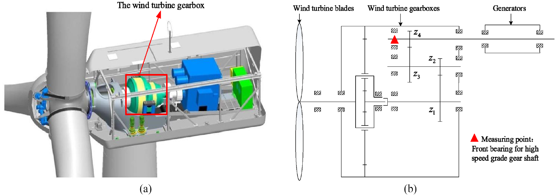
Structure and measurement point of wind turbine. (a) Wind turbine structure diagram and (b) measurement point.
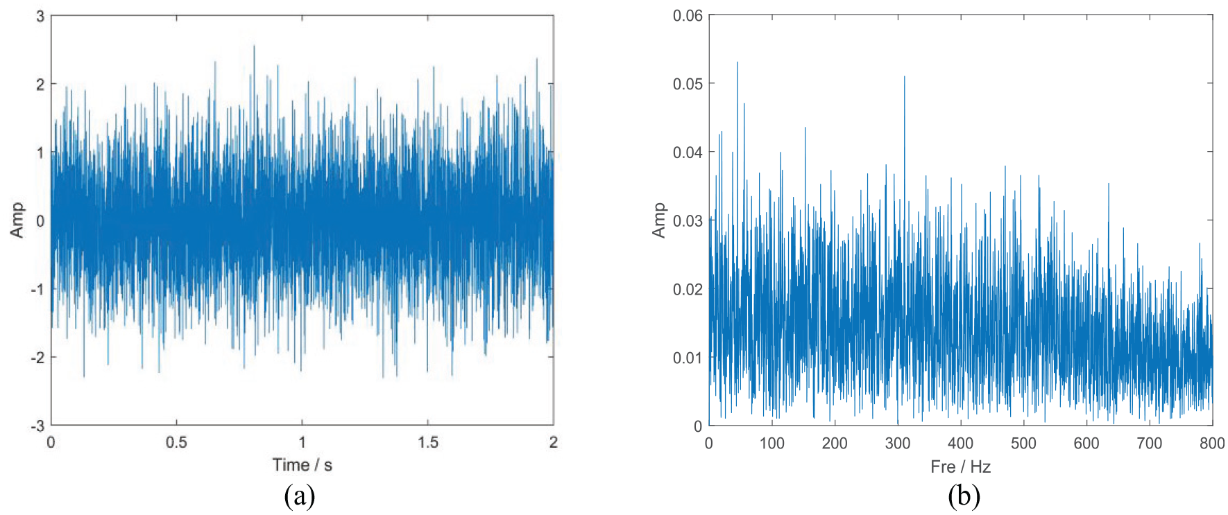
Vibration signal and its frequency spectrum from the wind turbine. (a) Vibration signals from the wind turbine and (b) frequency spectrum of vibration signal.
As the gearbox is operated at variable speed, it is not possible to identify the fault characteristics in the frequency spectrum from Figure 13(b), therefore a TFA is required to obtain more information about the fault under variable speed. In the search for fault characteristic frequency components, the interest frequency band range is set to
Four different algorithms were employed to analyze and calculate the wind turbine gearbox vibration signal and the results were demonstrated in Figure 14. By comparison, it is clear that the TFR of STFT and SST results have different degrees of energy divergence. Due to the strong oscillations encountered in the FIF decomposition for the original IMFogram, the time–frequency characteristic curve experienced periodic spurious fluctuations as presented in Figure 14(e) and (f). Instead, the proposed AIMFogram avoids this situation, as shown in Figure 14(g) and (h). The initial population size of the particle swarm is 50, the inertia weight
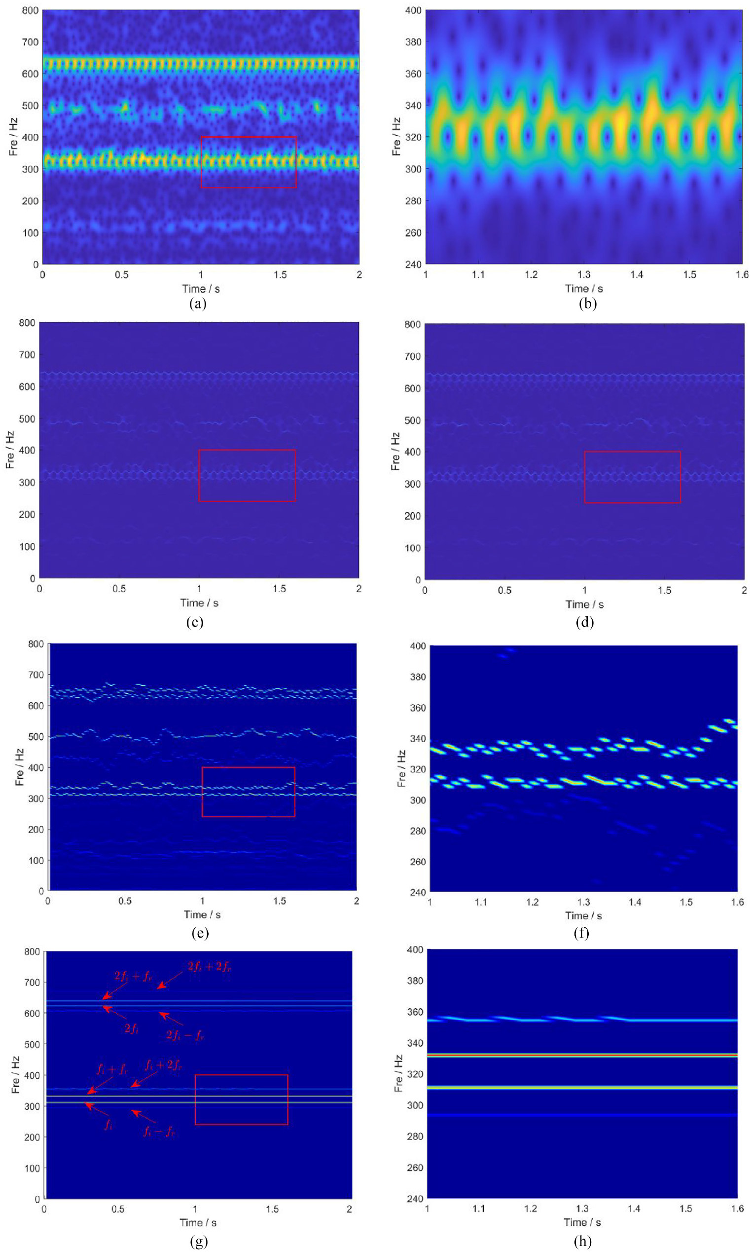
TFR of the wind turbine gearbox vibration signal for four different methods.
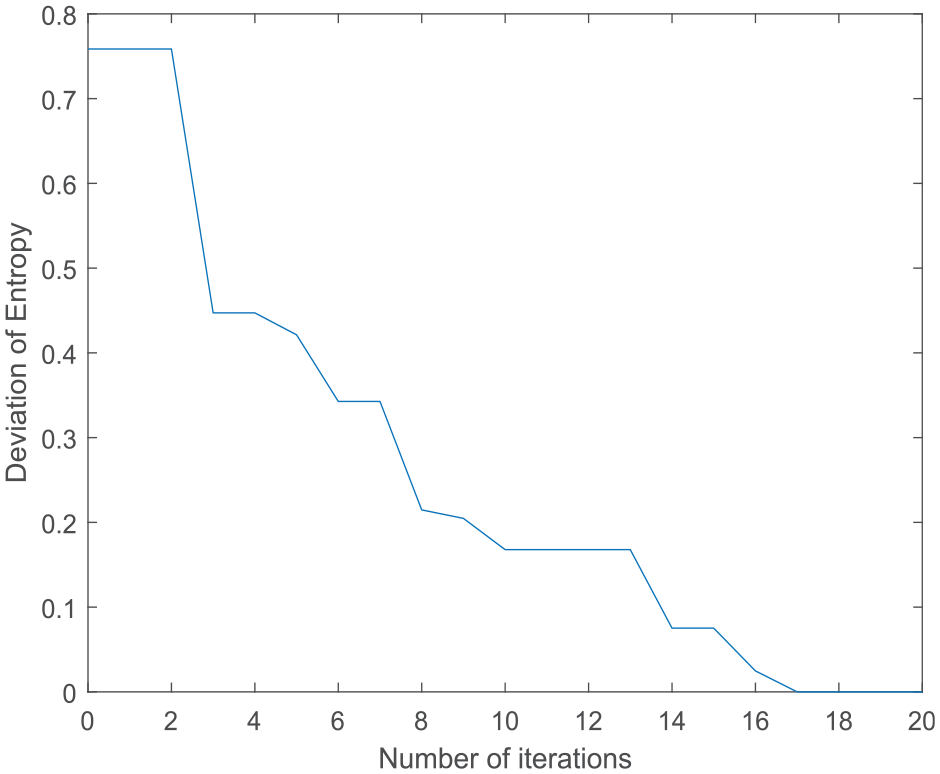
Variation of entropy difference with the number of iterations.
By querying the measurement records of the generator’s rotational speed, which was approximately n = 1250 rpm, the rotating frequency was calculated to be
Failure characteristic frequency of bearing in wind turbine gearbox.
Conclusion
In terms of the wind turbine gearbox under changing operating environment, this paper proposed the AIMFogram to achieve an accurate TFR of multi-components vibration signals aiming at the blurred TFR and hard extraction of signal fault characteristics. The main points of this paper are summarized as following: (1) Original FIF is replaced by an improved VNCMD, and a multi-ridge line detection method of MRD provides the ICF for the VNCMD, enabling adaptive decomposition of the signal without prior knowledge, which is more conducive to the vibration signal analysis under varying velocity. (2) PSO algorithm is employed to optimize the parameters of the structural element scale of the existing IMFogram, and the Renyi entropy is set as the fitness function so as to obtain the best scale parameters. (3) Furthermore, the proposed AIMFogram in this paper has successfully achieved fault diagnosis of a rolling bearing outer ring in a test bench and fault characterization of a gearbox in a 850-kW wind turbine. All the results above fully demonstrate the feasibility of proposed AIMFogram in this paper for rotating machinery fault diagnosis under varying speeds.
Footnotes
Declaration of conflicting interests
The author(s) declared no potential conflicts of interest with respect to the research, authorship, and/or publication of this article.
Funding
The author(s) disclosed receipt of the following financial support for the research, authorship, and/or publication of this article: This work is supported by Hubei Province Key Research and Development Plan (2021BAA194) and Guangxi Key Research and Development Plan (Guike AB21075009). Numerical calculation is supported by High-Performance Computing Center of Wuhan University of Science and Technology.