
Abstract
Deep learning-based concrete defect detection has emerged as a promising technology to overcome the limitations of manual visual inspection, which is often subjective, laborious, and time-consuming. However, most existing methods rely heavily on manual labels and adopt a fully supervised learning approach, which hinders their practical application in engineering. To tackle these concerns, we proposed a semi-supervised learning model, termed Semi-SegDefect. Our proposal utilizes a mean teacher architecture to assign pseudo-labels to the pixels of unlabeled images and performs pixel-level contrastive learning on a sparse set of hard negative pixels to achieve segmentation boundaries with the highest possible accuracy. Test results demonstrate that Semi-SegDefect outperforms fully supervised models significantly, especially when trained with limited labeled data. This method shows great promise for enhancing the accuracy and scalability of concrete defect segmentation and can contribute to the advancement of the construction industry.
Keywords
Introduction
Concrete structures are vulnerable to various defects caused by factors such as material aging, thermal stress, overloading, and inadequate maintenance, which can result in loss of functionality and safety hazards in infrastructure systems.1–3 Regular inspections are crucial for evaluating the current condition of structures and guiding decisions about defect maintenance. Although expert-dependent visual inspection has traditionally been used for detecting defects in concrete structures, this method tends to be time-consuming, labor-intensive, subjective, and prone to errors in many situations.4,5
Recently, the advancements in visual sensing technologies and machine learning have revolutionized operations across various industries. The civil infrastructure inspection and monitoring are also undergoing a transformation from manual visual inspection to data-driven automation, with the potential to achieve more efficient and automated infrastructure maintenance. 6 Machine learning provides advanced mathematical frameworks and algorithms capable of discovering and modeling structural performance and conditions from rich monitoring data sources like images and videos. 7 For concrete defect detection, computer vision techniques can facilitate long-distance, non-contact, low-cost, and automated detection, and many significant researches have been successfully explored. A proposal was made for a deep learning model that integrates One-Dimensional Convolutional Neural Network (1D-CNN) and Long Short-Term Memory (LSTM) to enhance computational efficiency. 8 The input images were transformed into the frequency domain, followed by calibration using the flattened frequency algorithm, and LSTM was employed to enhance the model’s performance on long sequence data. Complex backgrounds may weaken the robustness of convolutional neural networks, such as shallow cracks in range images. Heterogeneous image fusion can reduce false detections and achieve better classification performance. 9 Moreover, a robust augmentation strategy was proposed in Palevičius et al. 10 that includes ray-tracing of shadows, augmenting shadow datasets, and blending shadows, which significantly enhanced the detection robustness. Li et al. 11 proposed a crack detection model that employs enhanced preprocessing, coarse crack localization, and fine crack edge identification progressively. To increase the model’s sensitivity to noise in crack images, a combination of convolutional layers and a cycle generative adversarial network (GAN) was employed. 12 During the training process, multi-scale and multi-level features were aggregated, resulting in improved crack detection capabilities. To facilitate the detection of failures and the assessment of damages in reinforced concrete structures, YOLOv4 was introduced by Zou et al. 13 This model can detect and localize damage in these structures, thereby aiding in their quick and efficient assessment. Santos et al. 14 employed an unmanned aerial system to capture images of exposed steel bars on concrete structures. These images were then analyzed using a region-convolutional neural network (R-CNN), demonstrating the high adaptability of the deep learning-based method. Zhang et al. 15 presented a context-aware crack segmentation network that utilized a context-aware fusion technique with local cross-state and cross-spatial restrictions to integrate image patch predictions. Han et al. 16 used a convolutional neural network to find surface cracks in concrete structures and then modified a threshold method to extract clear crack contours for quantification. To further enhance model performance, researchers have turned their attention toward the use of attention mechanisms. These mechanisms are crucial in effectively utilizing crack features while suppressing background features, resulting in improved overall performance of the model. ATCrack 17 achieved pixel-level crack detection by applying channel spatial attention, increasing model accuracy and robustness. STRNet, 18 a network consisting of a squeeze and excitation attention-based encoder, a multi-head attention-based decoder, coarse up-sampling, and a focal-Tversky loss, showed rapid processing speed on concrete crack images. In addition, Cui et al. 19 proposed an improved attention mechanism model termed Att-Unet, which focused on critical areas, reconstructed semantic features, and significantly improved the pixel-level crack segmentation performance. MaDnet 20 simultaneously identified material types and fine/coarse structural damage via semantic segmentation. The network leverages shared filters learned through multi-objective optimization, improving accuracy. A modified fusion network was utilized to handle multi-level and multi-scale features. The method addresses real-world crack identification within steel box girders of bridges using images containing complex disturbances. 21 To identify and locate various seismic damages in images of damaged reinforced concrete columns, the modified Faster R-CNN was proposed, and the model’s effectiveness in recognizing specific damage types was analyzed. 22
The deep learning models presented in the aforementioned studies heavily depend on high-quality training labels. Semi-supervised learning leverages both labeled data and unlabeled data to extract supervised information. This technique has garnered considerable interest in recent years owing to the availability of vast amounts of unlabeled data in various real-world applications, as well as the desire to minimize the expenses and time involved in manual annotation. Shin et al. 23 combined multi-scale segmentation networks, discriminator networks, and adversarial learning to achieve crack detection in underground concrete structures. By generating a new precisely labeled image from unlabeled images, this approach reduces the burden of manual annotation while enhancing the segmentation performance. They subsequently combined a super-resolution network with a semi-supervised model, using a super-resolution network to improve the quality of the input image. 24 Another semi-supervised approach 25 was to generate supervision signals for unlabeled pavement crack images and use them for model training to compensate for insufficient image labels. Then, an adversarial strategy and a fully convolutional discriminator were employed to distinguish ground truth from predictions. The semi-supervised model also exhibited good robustness in the detection of steel surface defects. 26 An effective improvement for GAN-based semi-supervised models is to boost the performance of the generator. Gao et al. 27 proposed CU-Net and FU-Net based on the U-Net, which served as a generator to generate synthetic crack images, and the binary network was utilized as a discriminator. Wang and Su 28 proposed a semi-supervised model that utilizes consistency regularization for concrete crack segmentation. A few-shot meta-learning paradigm was introduced for structural damage identification. 29 The method involves an external few-shot meta-learning module and an embedded internal attribute-based transfer learning model. Compared to traditional supervised learning, it exhibits higher accuracy and robustness. Xu et al. 30 proposed a task-aware meta-learning approach, which includes an interpretable task generation strategy and a dual-stage optimization framework. The method is evaluated on a multi-type structural damage dataset, showcasing great performance even with limited training images.
While open-source datasets have contributed significantly to the field of concrete defect identification based on images, and high precision has been achieved in recognizing various defects, our main objective focuses on addressing two key challenges, making the transition to practical engineering applications smoother: (1) Reducing annotation effort: Despite the availability of open-source datasets, labeling data for specific engineering projects can be time-consuming and costly, especially when dealing with large-scale or specialized datasets. Our semi-supervised approach, Semi-SegDefect, offers a solution to minimize the need for extensive manual labeling, making it more practical for real-world scenarios. (2) Enhancing performance: Semi-SegDefect has demonstrated superior performance, especially when trained with limited labeled data. This is significant because in practical engineering scenarios, acquiring a vast amount of labeled data may not always be feasible or cost-effective. Our approach improves the accuracy of defect identification even when data availability is limited. Furthermore, the model proposed in this study exhibits excellent scalability. In real-world engineering scenarios, when encountering new types of defects that were not originally considered during the model’s development, our approach offers a practical advantage. With only a small amount of labeled data specific to the new defect type, our model can efficiently adapt and generalize its defect identification capabilities. This adaptability to novel defect categories is a valuable feature, as it allows for the continuous improvement and versatility of the model in addressing emerging challenges within the construction industry. In this study, we proposed a semi-supervised model for pixel-level detection of crack, spalling, and rebar exposure, which improves model performance by providing appropriate contrastive supervision information. Our contributions can be summed as follows:
A semi-supervised learning framework is proposed for multi-class defect segmentation of concrete structures.
Pixel-level contrastive learning is utilized to help models learn feature information from both local context and global semantic class relationships across the entire dataset.
Active sampling strategy optimizes only a sparse set of queries and keys, avoiding expensive computation costs.
Compared with fully supervised methods, our proposal achieves superior results with very few labels.
Methodology
General description
Based on strategies such as consistency regularization, 31 entropy minimization, 32 and pseudo-labeling, 33 many semi-supervised models have been proposed for semantic segmentation. The essence of these strategies is that the model output should always maintain a low-entropy prediction for data perturbations and geometric transformations. Inspired by these approaches, we have developed a semi-supervised segmentation model, Semi-SegDefect, based on pixel-level contrastive learning. Figure 1 depicts the overall structure of our approach, which comprises three components: supervised loss calculation, unsupervised loss calculation, and pixel-level contrastive loss calculation. The computation of supervised loss is implemented by feeding the ground-truth data into the student model. The unsupervised loss calculation adopts Mean Teacher architecture, 34 which includes two fundamental networks: the student model and the teacher model. The pixel-level contrastive loss calculation of concrete defects is performed by projecting the prediction results of labeled and unlabeled data into a high-dimensional feature space. For the improvement of semi-supervised segmentation models, diverse data perturbations are crucial. The strong augmentation process involves the sequential use of color dithering, Gaussian filtering, and CutMix methods. Weak augmentation only includes random flipping and random cropping. Details of each component are elaborated as follows.
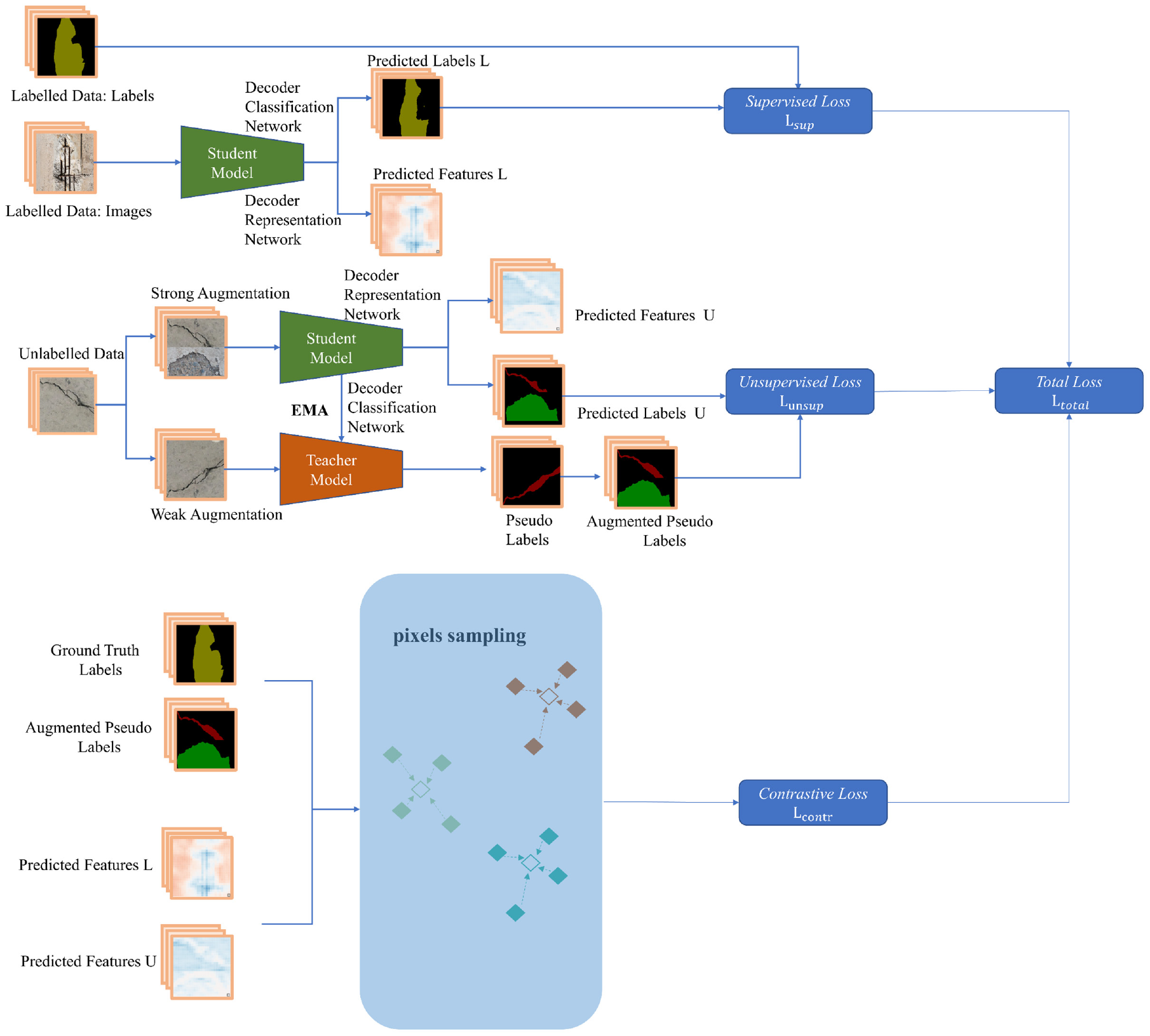
The overall structure of Semi-SegDefect.
Mean teacher framework
The structure of Semi-SegDefect is modified based on Mean Teacher. 34 Mean Teacher architecture adopts the consistency regularization strategy, where the model predictions should not change significantly if data perturbations are applied to unlabeled data samples. In the Mean Teacher architecture, the same network plays dual roles: teacher and student. As a teacher, the goal is to generate objects for consistency loss computation with unlabeled data as input. The teacher model and student model do not share weights. Instead, the teacher model employs the exponential moving average weights of the student model, as depicted in formula (1). This method enables the model to collect information after each training iteration, thereby enhancing the output of all layers for an improved intermediate representation. During the early training stages, the student model progresses rapidly, necessitating the teacher model to swiftly discard outdated and inaccurate student weights. As training progresses and the student model’s progress slows down, the teacher model can benefit from a longer memory by adjusting the smoothing coefficient hyperparameter.

where
Student model and teacher model
Both the student and teacher models adhere to the traditional encoder–decoder structure for semantic segmentation, as shown in Figure 2, and they share the same architecture. The encoder extracts image features by increasing the number of channels while decreasing the resolution, resulting in a pyramid feature structure with four distinct scales. The decoder then projects the semantically rich features into pixel space to produce dense classification results. An input image undergoes a convolution operation with a 4 × 4 kernel and a stride of 4 for a quick reduction in resolution (4× down-sampling) and an increase in channel number from 3 to 192, without information loss. The down-sampled feature maps are then processed by the ConvNext block 35 for further feature extraction, producing the output of the first encoder stage. The following three stages use a convolution operation with a 2 × 2 kernel and a stride of 2 for 2× down-sampling prior to feature extraction. The final feature map resolutions correspond to 1/4, 1/8, 1/16, and 1/32 of the input image, respectively. The ConvNext block, depicted in Figure 3, is the key component of the encoder and extracts image features by stacking multiple convolutional layers.
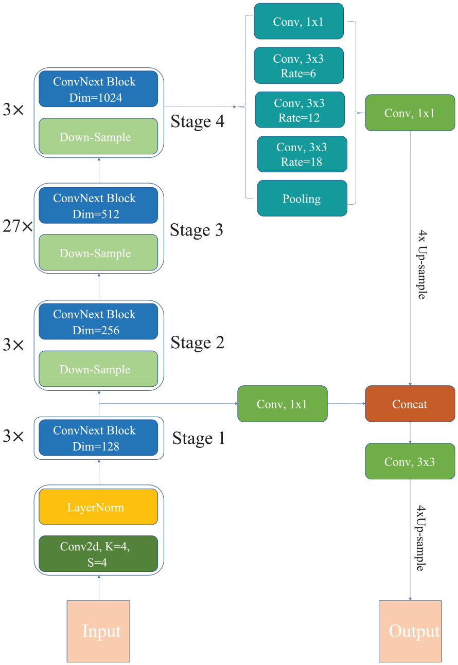
Student model and teacher model structure.
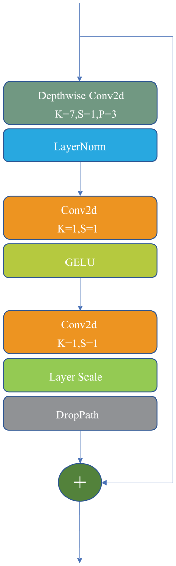
ConvNext block.
The ConvNext block first uses a depth-wise separable convolution with a kernel size of 7 × 7, a stride of 1, and a zero padding of 3 for feature extraction. Compared with standard convolution, depth-wise separable convolution greatly reduces the number of parameters. Then two convolution kernels with a size of 1 × 1 and a stride of 1 are used to realize dimension increase and reduction of feature maps, respectively. The dimension increase operation multiplies the number of input channels by four, allowing for the extraction of more semantically rich information from the feature space.
The decoder employs an atrous spatial pyramid pooling (ASPP) 36 for feature extraction across different receptive fields. It has five parallel branches, consisting of a 1 × 1 convolutional layer, three 3 × 3 dilated convolutional layers, and a global average pooling layer. The ASPP effectively captures multi-scale information using parallel convolution layers with different atrous rates, making the model perform better on multi-scale objects. The outputs from the five branches are concatenated along the channel direction and further fused through a 1 × 1 convolutional layer that adjusts the channel number. To utilize position information in low-dimensional features, a 1 × 1 convolution compresses the low-level feature channels from Stage 1 to 48 channels, providing a bias toward higher-level semantic information. After 4× up-sampling, high-dimensional features are concatenated with low-dimensional features. The output is obtained via a 3 × 3 convolution and bilinear up-sampling.
Pixel-level contrastive learning
Contrastive learning has gained significant success in recent years. It leverages the entirety of information in the dataset to learn a highly representative image representation space. In semantic segmentation, the labels of each image are already known, and positive samples can be considered as pixels of the same category while negative samples can be considered as pixels of different categories, regardless of whether they come from the same image or not.37,38 Contrastive learning can be utilized to enhance the traditional cross-entropy loss by discovering the global semantic relationship between pixels across all the training images, thereby producing a structured semantic feature relationship.
The cross-entropy loss at the pixel level is a standard loss function in semantic segmentation. This loss guides the network on whether its predictions for individual pixel classes are accurate. Despite its usefulness, the cross-entropy loss does not consider the local information of neighboring pixels or the relationships between errors in different classes. To address this, a more effective approach would be to design the loss function to leverage the relationships between categories. Rather than simply teaching the model to identify individual pixels as cracks or spalling, a better approach would be to provide finer supervision on easily confused pixel categories. The availability of finer supervision allows the model to learn more discriminative features in a semi-supervised setting, even with limited labeled data, resulting in improved overall segmentation performance.
To improve the feature representations learned by the model in semi-supervised segmentation, we have incorporated pixel-level contrastive learning that offers insight into the relative relationships between various semantic categories. Suppose
For an anchor pixel
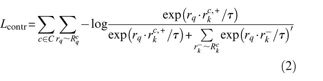
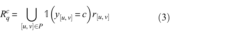
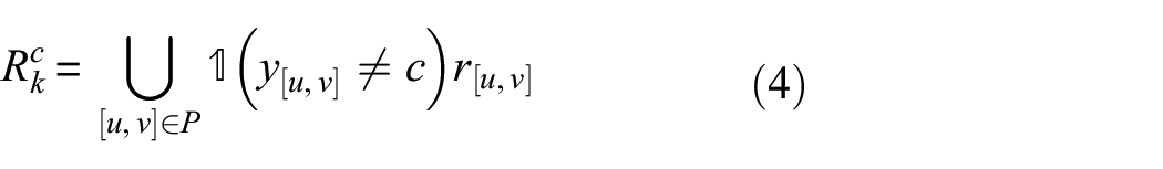
where C is the set of all categories contained in the current batch size;
Suppose P is a set that contains all pixel coordinates with the same resolution as R, these anchor pixels, negative pixels, and average representation used for the contrastive loss calculation can be formulated as follows:
Loss function
Two data sources are available for training semi-supervised semantic segmentation models: a limited number of labeled samples

where
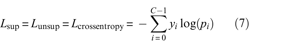
Labeled data are used for the calculation of supervised loss during training, which compares the model’s predictions on labeled data to the ground truth labels and is crucial for training the model to make accurate predictions on these labeled examples. The unsupervised loss is calculated based on unlabeled data, with the purpose of encouraging the model to produce consistent predictions on different views or augmentations of the same unlabeled data point. This consistency regularization helps improve the model’s robustness and generalization. Finally, the pixel-level contrastive loss is calculated based on the dense representations predicted from labeled and unlabeled images. Contrastive loss is applicable to all pixels in labeled samples and valid pixels in unlabeled samples. Valid pixels in unlabeled samples are those located in the pseudo-labels with category confidence greater than a threshold
Data preparation and augmentation
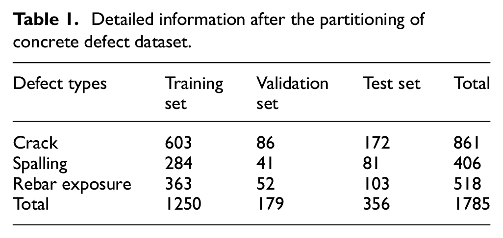
The dataset is a crucial component in the development and training of segmentation models, as the model performance is closely tied to the quality and quantity of the data it is trained on. In recent years, many concrete defect datasets have been made public, which facilitates the conduct of experiments.39–42 We collected relevant datasets, cropped the original image into sub-images with a resolution of 512 × 512 pixels, and only kept the images containing concrete defects. Cropping to a smaller size can ensure that the model only learns the most important information, reducing the risk of overfitting and improving its generalization capabilities. In addition, cropping to a smaller size also reduces the computational cost of training as it requires less memory and processing power. In this way, 1785 images were finally obtained. Unlike classification tasks that rely on extensive datasets like Imagenet or COCO, the focus of our research is defect segmentation, where the emphasis is on pixel-level precision rather than recognizing object classes in entire images. The dataset size depends not only on the number of images but also on the number of pixels within each image, which determines the quantity of training samples available during model training. In the image semantic segmentation task, each pixel can be considered an individual training sample because our goal is to assign the correct semantic label to each pixel. This means that even if the dataset contains limited images, the data volume is still ensured, as every image comprises hundreds of thousands of pixels, each of which provides valuable training information. Hence, even with a dataset containing limited images, considering each pixel as an individual training sample provides the model with a sufficient amount of information to learn various semantic features and boundaries accurately. This fine-grained level of annotation is essential for achieving precise image semantic segmentation, and as such, the data volume is indeed guaranteed. To evaluate the model performance, the dataset is randomly split into training, validation, and test sets in a ratio of 7:1:2. Table 1 summarizes the details of each type of defect in the dataset. In the dataset, crack defects tend to have fewer crack pixels per image, making them more challenging to detect, and therefore, fewer training samples are available compared to the other two defect types. By contrast, spalling and rebar exposure defects typically cover larger areas within the images, making them relatively simpler to detect. Therefore, there are more training samples for crack detection to facilitate comprehensive feature extraction. This distribution accounts for the varying complexities of defect types and aims to ensure effective model training for each category. Figure 4 shows several samples in the concrete defect dataset.
Detailed information after the partitioning of concrete defect dataset.
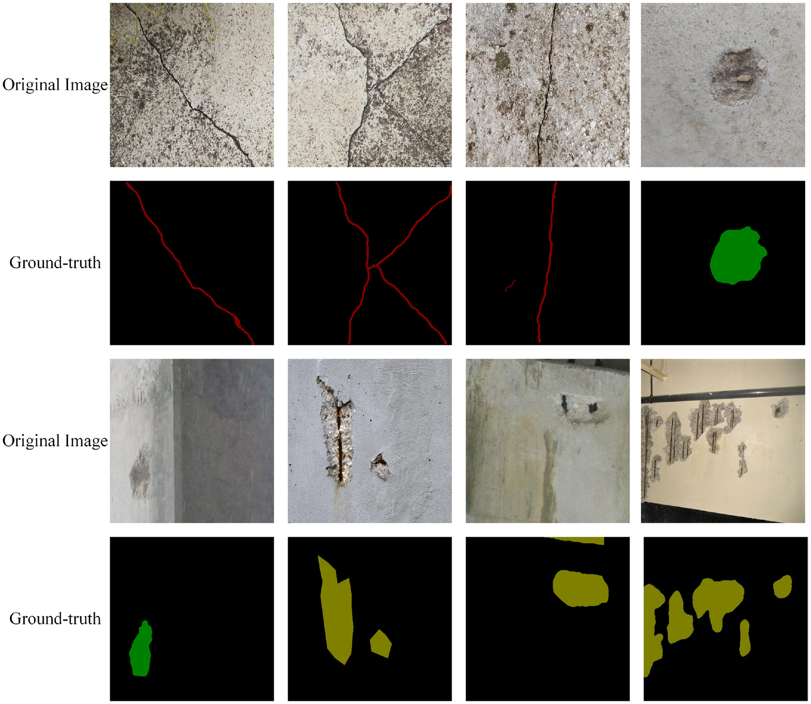
Samples in the concrete defect dataset.
Traditional data augmentation techniques, while valuable for enhancing model generalization, often fall short in the context of semantic segmentation. These methods primarily apply isolated transformations to individual images, which can disrupt the spatial relationships crucial for accurate segmentation. By contrast, CutMix
43
addresses these limitations by seamlessly blending segments of different images. This approach yields several notable advantages: First, CutMix introduces a contextual understanding that traditional data augmentation methods cannot match. By combining segments of multiple images, the model learns to recognize how different objects and regions within an image relate to one another. This heightened contextual awareness leads to improved semantic segmentation. Second, the regularization effect of CutMix is remarkable. The act of replacing segments from one image with those from another enforces consistency within the mixed regions. This regularization discourages overfitting and encourages the model to produce stable predictions. In a semi-supervised setting where labeled data are often scarce, this regularization proves invaluable for effectively leveraging the limited labeled examples. Moreover, by blending regions from distinct images, it guides the model toward learning more accurate and refined segmentation boundaries. CutMix mixes two images along with their corresponding labels to form a new, combined image and label, as shown in Figure 5. By training on a diverse set of images and labels, including those created through CutMix, the model can learn to handle ambiguous and challenging data more effectively. The combined image is a mix of two input images, and the combined label is a mix of their corresponding segmentation masks. The segmentation masks can be combined in the same way as the images, by randomly selecting two regions and merging them to form a single mask. Assuming that

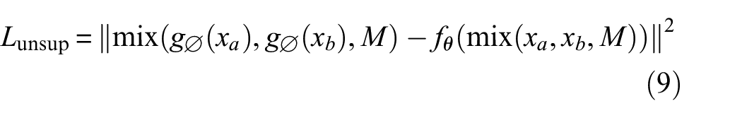
where
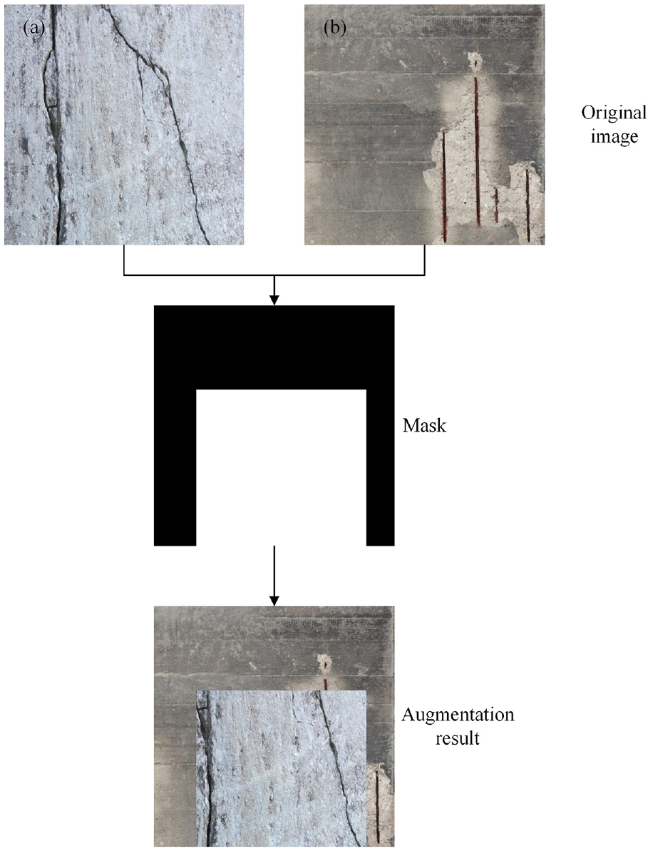
Schematic diagram of CutMix.
In the CutMix algorithm,
Implementation details
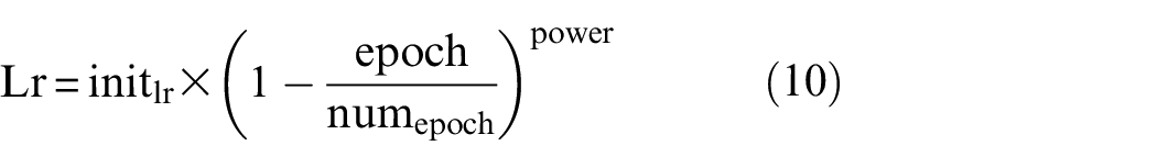
To assess the efficacy of semi-supervised learning, we trained and tested the Semi-SegDefect model on the dataset established in the section “Data preparation and augmentation.” The model was trained and tested on a PC running the Win10 operating system with an Intel® Core™ i7-8700 CPU and a GeForce GTX 1080 Ti 11GB GPU. To ensure fair comparisons, the validation and test sets were kept consistent throughout the experiments. During training, the AdamW 44 optimizer was utilized with an initial learning rate of 1e-3, and a batch size of 2. During the early stage of training, a higher learning rate is recommended to allow the network to converge quickly. Conversely, a lower learning rate is recommended during the later stage of training to enable the network to converge toward an optimal solution more accurately. To achieve this, the Poly strategy was employed to dynamically adjust the learning rate using a power of 0.95.
The quantitative evaluation of the segmentation model adopts two popular metrics: Intersection over Union (IoU) and Mean Intersection over Union (MIoU). IoU is the area of overlap between the predicted segmentation and the ground truth divided by the area of union between the predicted segmentation and the ground truth. MIoU is the average IoU across all classes in a dataset. This metric provides a more comprehensive view of model performance, as it takes into account the performance of individual classes. Figures 6 and 7 show the learning rate and MIoU curves during training. MIoU first increases over time. At some point, the model reaches a saturation point, where the MIoU does not improve significantly despite further training. This indicates that the model has reached its maximum performance capacity, and further training may not result in significant improvements, which will be used for further estimation of model performance:
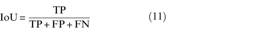

where TP refers to the number of pixels that are correctly classified by the model as belonging to a certain defect class; FP refers to the number of pixels that are wrongly classified by the model as belonging to a certain defect class when they actually do not; FN refers to the number of pixels that belong to a certain defect class but are misclassified as another class or as background by the model.
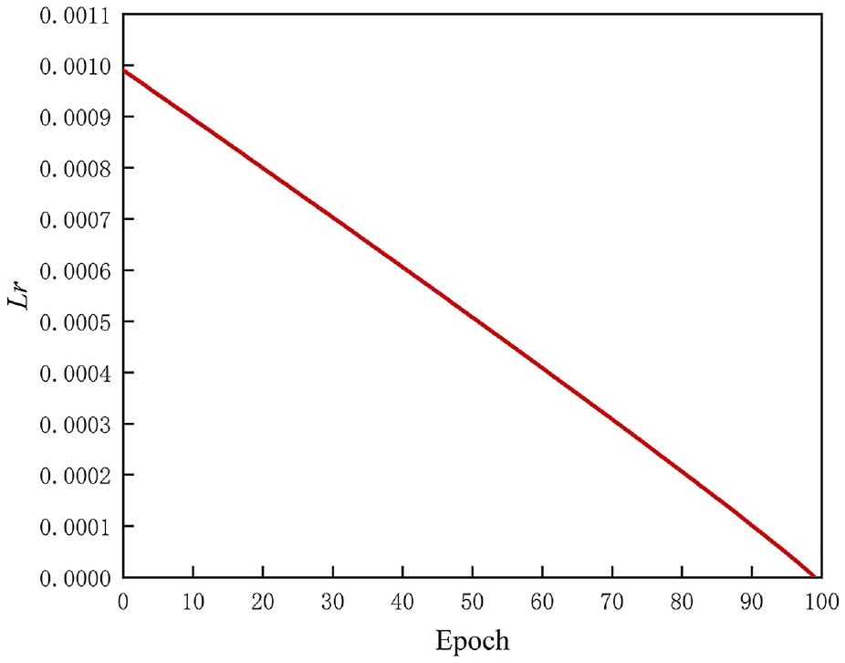
The curve of learning rate during training.
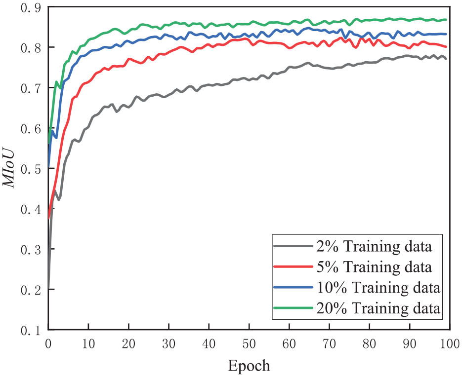
Curves of MIoU during training.
Test results and discussion
Selection of initial learning rate
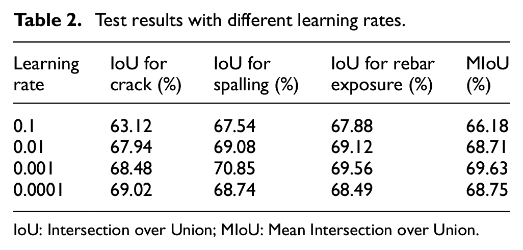
Learning rate is a hyperparameter that determines the step size at which the model updates its parameters during the training process. It is an essential factor in determining the model’s convergence and performance. The ideal learning rate value depends on the problem and the dataset at hand. A learning rate that is too small can result in slow convergence of the model, while a learning rate that is too large can cause the model to overshoot the optimal solution and lead to divergence. This section tests the performance of the model by setting different initial learning rates. Table 2 presents the segmentation results in terms of IoU scores for each category at different learning rates. The MIoU is also calculated to provide an overall performance measure. According to the values in the table, it can be found that when the learning rate is set to 0.1, the performance of the model is the worst. This is mainly because a large learning rate makes the training process of the model divergent and cannot achieve the global optimum. As the learning rate decreases, the optimization process converges more slowly but is more likely to find the global optimum, achieving the best performance with an MIoU of 69.63% when the learning rate is set to 0.001. However, if the learning rate is too small, the optimizer may take tiny steps that cause the model to converge too slowly or get stuck in a local minimum, leading to underfitting. This can result in poor segmentation performance, where the model fails to capture the necessary details in the input data for accurate segmentation. Therefore, the initial learning rate is uniformly set to 0.001 in the following experiments.
Test results with different learning rates.
IoU: Intersection over Union; MIoU: Mean Intersection over Union.
Impact of contrastive loss weight on model performance
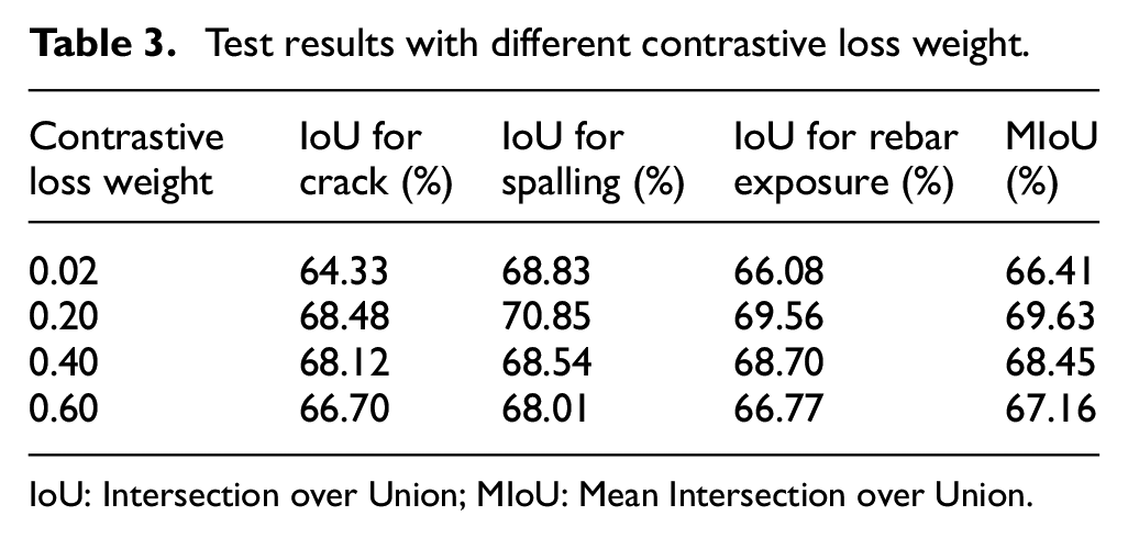
The weight assigned to the contrastive loss function in semi-supervised learning is crucial in determining the balance between the supervised and unsupervised components. The objective of contrastive loss is to enhance the similarity between positive pairs of instances while minimizing the similarity between negative pairs of instances within the feature space. It is a measure of similarity between pixels of different defect categories. In practice, the weight of the contrastive loss function is typically set through experimentation and tuning. To balance the contribution of contrastive loss and the other two losses to the total loss, a hyperparameter study is carried out by setting different loss weights, and the results are summarized in Table 3. It indicates that as the weight of the contrastive loss increases, the total loss gives more weight to the differences between pixel categories. However, if the weight of the contrastive loss becomes too large, it may dominate the total loss and cause a decrease in the overall segmentation performance of the model. Therefore, the contrastive loss weight is set to 0.20 in the experiment.
Test results with different contrastive loss weight.
IoU: Intersection over Union; MIoU: Mean Intersection over Union.
Impact of unsupervised loss weight on model performance
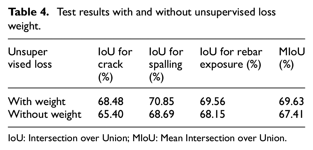
It is beneficial for training that the unsupervised loss weight starts close to zero because the initial model prediction accuracy is low, and the pseudo-labels at this time will not be a reasonable object to provide additional supervision information. Therefore, the contribution of unsupervised loss to the total loss should not be too big. As the training progresses, the model performance improves, and the weight can be increased at this time. In the experiments, the unsupervised loss weight is set as the percentage of the number of pixels with a confidence greater than 0.97 in the predicted pseudo-labels, as a sufficient representative of the prediction quality. The effect of unsupervised loss weights on model performance is shown in Table 4. The results indicate that when the unsupervised loss weight is not set, the segmentation performance of the model for crack, spalling, and rebar exposure drops by 3.08%, 2.16%, and 1.41%, respectively. Unsupervised loss contains much uncertain information, when the unsupervised loss weight is not set, all predicted pixel information will be used for model training, resulting in a great interference to the normal model training.
Test results with and without unsupervised loss weight.
IoU: Intersection over Union; MIoU: Mean Intersection over Union.
Impact of sampling strategy on model performance
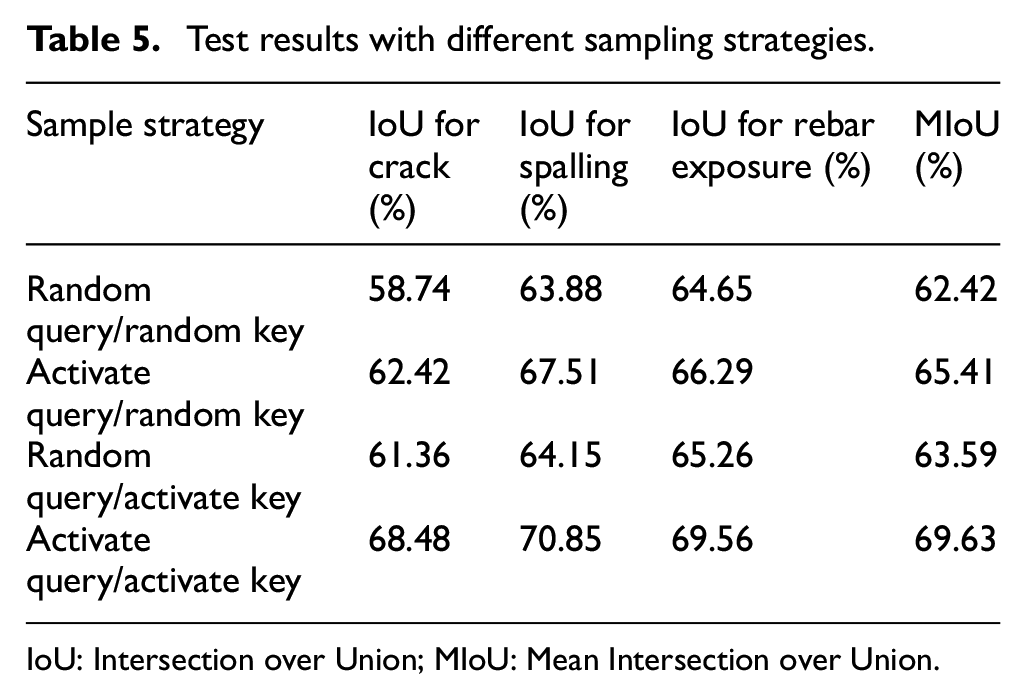
An image contains thousands of pixels, and sampling all the pixels when calculating pixel-level contrastive loss will bring huge computational costs and is unnecessary. The segmentation network is usually only indistinguishable for the pixels at the junction of different categories. To solve the above issue, an active sampling strategy is adopted. The active sampling strategy requires that the selection of anchor pixels must meet the following requirements: (a) under weak data augmentation, the model’s prediction confidence is greater than 0.7 and (b) under strong data augmentation, the model’s prediction confidence is less than 0.97. The anchor pixel first needs to be guaranteed to have the correct label. For the pixels from the labeled dataset, the correctness of the label can be guaranteed; for the pixels from the unlabeled dataset, the requirement (a) can ensure that those pixels with reliable prediction are selected. Requirement (b) can ensure that the model can sample indistinguishable pixels, and only the gradient update of these pixels with insufficient confidence can really help improve performance. If we sample anchor pixels with confidence greater than 0.97 for comparative learning under strong data augmentation operations, the model will not learn any useful information because models have learned well at the beginning for simple samples.
When sampling negative samples, it is better to select those pixels that are easy to confuse, and the definition of these confusion categories obviously cannot be artificial because the confusion categories may be different in different training stages. In the experiment, non-uniform sampling is performed by calculating the relative distance between defect pixels of different categories. If the distance is close, it is considered to be a confusion category. The calculated distances can form a probability distribution where negative samples are sampled. This process assigns more negative samples to categories that are easy to confuse, helping the model learn more accurate decision boundaries.
Table 5 summarizes the model performance when trained with different sampling strategies. Compared with the active sampling strategy, when the random sampling strategy is used, the IoU of crack, spalling, and rebar exposure drops by 9.74%, 6.97%, and 4.91%, respectively, mainly due to that the randomly sampled pixels contain a large number of simple samples. The model fails to learn useful knowledge from these simple samples through contrastive learning, and the effect of contrastive loss cannot be reflected. If the random key is replaced by the activate key, the performance improvement of the model is still small, and the MIoU only improves by about 1.17%. The activate query strategy has a major impact on the model performance, which further confirms that most queries are redundant.
Test results with different sampling strategies.
IoU: Intersection over Union; MIoU: Mean Intersection over Union.
Influence of sampling quantity on model performance
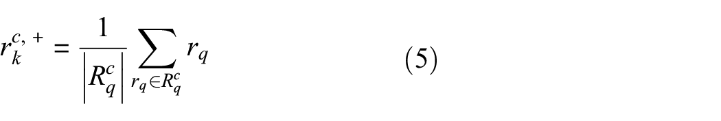
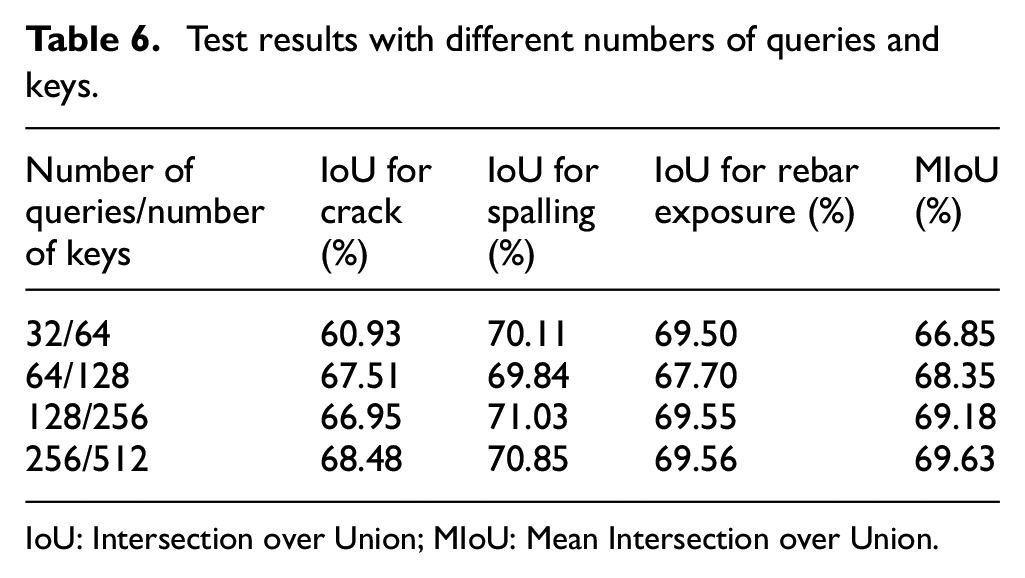
The pixels used for contrastive loss calculation are sampled from the decoder representation network, including three categories: anchor pixels, positive pixels, and negative pixels. Positive pixels are represented by the average representation of the class, calculated by Equation (5). Anchor pixels are selected for comparison with other pixels in an image to learn representations that keep the anchor pixels close to other pixels in the same class and far from pixels in different classes. The number of anchor pixels and negative samples chosen can impact the performance of contrastive loss functions in semi-supervised learning. Typically, the number of anchor pixels is smaller than the number of negative samples in practical applications since negative samples often contain difficult-to-classify pixels that can improve model performance. This ensures that the contrastive loss function has enough negative samples to learn from. As the number of pixel samples increases, the computational cost also increases. The number of pixel samples required depends on the dataset’s complexity and the neural network architecture used for training. This part studies the change in model performance by setting different numbers of anchor pixels and negative pixels. The number of negative samples is set to be twice of anchor pixels. The results are shown in Table 6. It can be observed from Table 6 that when the number of anchor pixels is too small, the model performance is not ideal due to the difficulty of contrastive loss to fully evaluate the difference between pixels of different defect categories. When sampling more pixels, the model performance will be better, but after a certain point increasing the number of sample pixels will have a small improvement in the segmentation performance. Considering the performance improvement and computer hardware requirements, the number of anchor pixels and negative samples is selected as 256/512. It is worth noting that in the four sampling settings, even with the smallest number of pixels (32/64), the segmentation result (MIoU 66.85%) is still better than the DeepLabv3+ shown in Table 9 (MIoU 60.47%), which further verifies the effectiveness of pixel-level contrastive learning.
Test results with different numbers of queries and keys.
IoU: Intersection over Union; MIoU: Mean Intersection over Union.
Comparison results across different dimensions of contrastive loss calculation
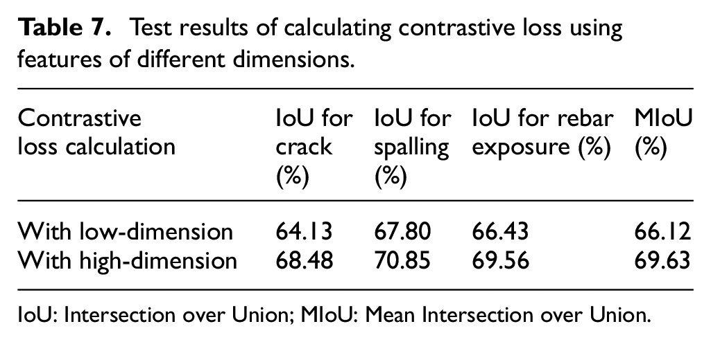
The encoding features extracted from the encoder network often reside in a lower-dimensional space, which might not capture the subtle nuances and semantic information crucial for tasks like similarity learning or contrastive loss effectively. The decoder representation network begins with a 2D convolutional layer using a kernel size of 3 × 3 to extract features. Subsequently, batch normalization is applied to stabilize training. An activation function, ReLU (Rectified Linear Unit), introduces non-linearity into the network. Lastly, another 2D convolutional layer with a 1 × 1 kernel further refines the features, transforming each pixel’s feature vector independently, resulting in the extraction of higher-level feature representations. Table 7 shows the segmentation performance when using high-dimensional features and encoder features for contrastive loss calculation. It can be seen that when high-dimensional features are used to calculate the contrastive loss, the IoU for crack, spalling, and rebar exposure are improved by 4.35%, 3.05, and 3.13%, respectively. By employing a separate decoder representation network that projects these features into a higher-dimensional space, we enrich the feature representations with more expressive power. This higher-dimensional space allows the model to distinguish subtle differences and similarities more effectively, leading to enhanced discriminative capabilities. Furthermore, using high-dimensional features before applying contrastive loss fosters better separability between positive and negative pairs. It provides the model with a broader feature space to work with, reducing the risk of feature collapse or over-regularization that can occur when using lower-dimensional representations directly. The increased dimensionality amplifies the model’s ability to capture fine-grained patterns. Therefore, employing a decoder representation network to project features into a higher-dimensional space before applying contrastive loss is both effective and necessary. It empowers the model with richer and more expressive feature representations and enhances its discriminative capabilities.
Test results of calculating contrastive loss using features of different dimensions.
IoU: Intersection over Union; MIoU: Mean Intersection over Union.
Effect verification of different loss branches
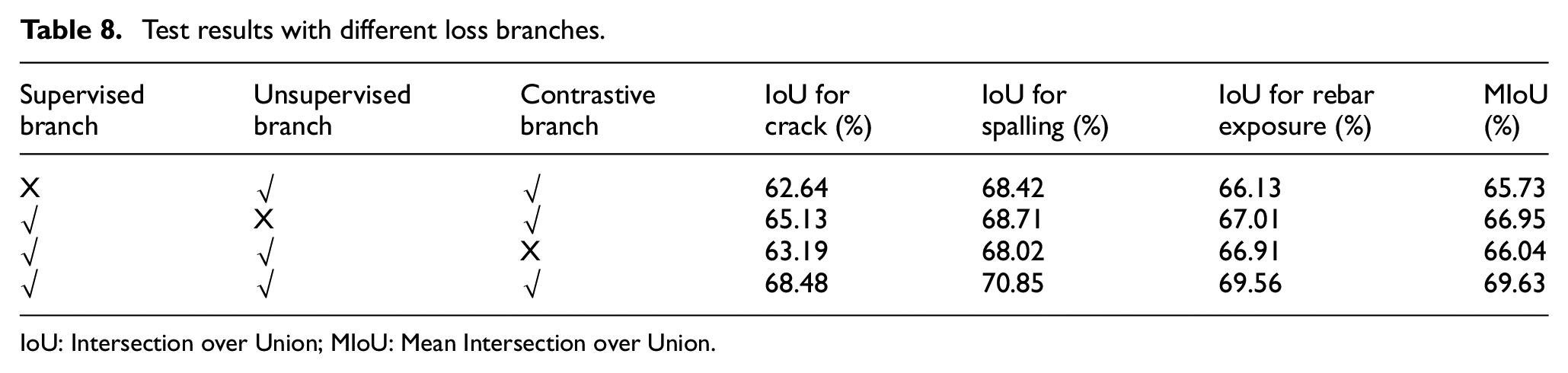
In this study, the loss function comprises three components: supervised loss, unsupervised loss, and contrastive loss. To assess the influence of each loss on model performance, we conducted ablation experiments, and the test results are summarized in Table 8. It can be seen that removing the supervision loss from the total loss will lead to a significant decrease in model performance, with the IoU of crack, spalling, and rebar exposure being reduced by 5.84%, 2.43%, and 3.43%, respectively. The supervised loss serves as a crucial source of task-specific guidance, ensuring that the model accurately predicts labeled data. In addition, the supervised loss aids in generalization, helping the model extend its learning from labeled examples to unseen data. Without it, the model will struggle to adapt to new, unobserved instances, reducing its overall effectiveness. The unsupervised loss leverages the information from unlabeled data, aiding in feature learning, and improving the model’s generalization capabilities. Its absence can lead to a reduction in the model’s ability to utilize unlabeled data effectively, resulting in overfitting to the labeled data. The contrastive loss encourages the model to bring similar samples closer together in feature space while pushing dissimilar samples apart. This mechanism helps the model better discriminate between different classes or objects and enhances its ability to capture subtle differences and similarities in the data. Without the contrastive loss, the model will struggle to learn discriminative features, which can lead to a reduction in its overall performance. When unsupervised loss and contrastive loss are not considered, the overall performance of the model decreases by 2.68% and 3.59%, respectively, in terms of IoU. A balanced combination of all three losses is critical for optimizing the performance of the model in concrete defect segmentation.
Test results with different loss branches.
IoU: Intersection over Union; MIoU: Mean Intersection over Union.
Comparative studies
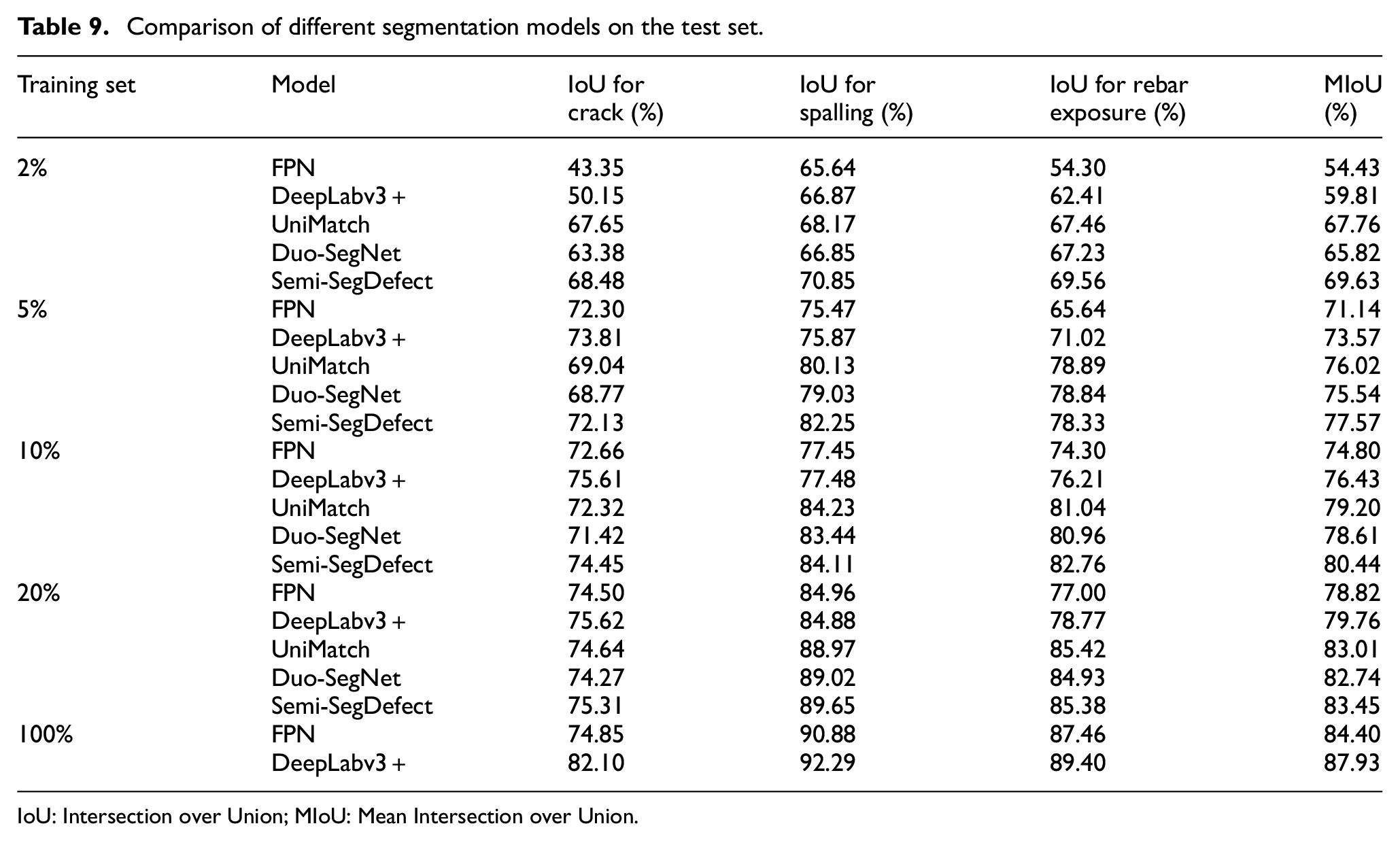
To ensure the fairness of the comparative studies, we took several measures to mitigate the risk of models getting stuck in the local optimum. First, we employed a consistent experimental setup for both the semi-supervised model (Semi-SegDefect, UniMatch, 45 and Duo-SegNet 46 ) and the fully supervised models (FPN, 47 DeepLabv3+ 48 ) by training them on the same subsets of the dataset—specifically, 2%, 5%, 10%, and 20%. This ensured that all models were exposed to equivalent data proportions, minimizing any potential bias stemming from varying dataset sizes. In addition, we implemented the same training strategies designed to help models escape local optimum, including using appropriate learning rate schedules and data augmentation techniques. These strategies aimed to encourage model convergence to more favorable solutions and avoid overfitting.
As shown in Table 9, Semi-SegDefect greatly outperforms DeepLabv3+ when training with 2%, 5%, 10%, and 20% of labeled data. The MIoU are increased by 9.82%, 4.00%, 4.01%, and 3.69%, respectively, which fully demonstrates that the proposed semi-supervised model can mine more effective semantic information from a large amount of unlabeled data to provide additional supervision information for the classification of defect pixels. When the model is trained with very few labeled data (2%, 25 labeled images), the performance gap between the fully supervised model and the semi-supervised model, Semi-SegDefect, is the largest, 18.33% for crack, 3.98% for spalling, and 7.15% for rebar exposure, respectively. The deep learning model has a large number of model parameters, and the model is prone to overfitting when only a few data are used for training, which affects the model’s robustness and generalization performance. Semi-SegDefect makes predictions on unlabeled data after training with a small amount of data and provides supervision information for the successive model training by selecting pixels with reliable predictions in pseudo-labels. When trained with a limited amount of labeled data, semi-supervised models consistently demonstrate superior performance compared to fully supervised models. While UniMatch and Duo-SegNet exhibit competitiveness, they generally exhibit lower IoU scores and MIoU compared to Semi-SegDefect, especially in scenarios with few labeled data. Under the conditions of 2%, 5%, 10%, and 20% labeled data, UniMatch exhibits MIoU scores that are lower than Semi-SegDefect by 1.87%, 1.55%, 1.24%, and 0.44%, respectively. Similarly, Duo-SegNet demonstrates MIoU scores that are lower than Semi-SegDefect by 3.81%, 2.03%, 1.83%, and 0.71%, respectively. The performance gap between the semi-supervised models narrows as the training set size increases, which can be attributed to the distinct strategies these models employ in leveraging unlabeled data. Each semi-supervised model relies on different mechanisms and assumptions about the distribution of unlabeled data, and these discrepancies become more evident when labeled data is scarce. With a larger portion of labeled images participating in the training, the models benefit more from the direct supervision provided by these labeled samples. In the case of spalling and rebar exposure, UniMatch may achieve higher IoU scores than Semi-SegDefect at times. However, its MIoU for all three defects is lower.
Comparison of different segmentation models on the test set.
IoU: Intersection over Union; MIoU: Mean Intersection over Union.
Figure 8 shows the segmentation results of the Semi-SegDefect model on the test set when using 20% labeled data for training. For visual comparison, the segmentation results of DeepLabv3+ trained with all labeled data are also given in Figure 8. Regarding the mis-segmented areas, both models tended to have difficulties in accurately detecting small or faint defects, resulting in under-segmentation. The semi-supervised model also had some mis-segmentation in areas with complex textures or ambiguous boundaries, possibly due to the limited amount of labeled data in the training set. By contrast, the fully supervised model was able to capture more details of the defects, but it still suffered from mis-segmentation in areas with similar edge texture or color to the background. Overall, it can be concluded that Semi-SegDefect can achieve satisfactory segmentation of defects with limited labeled data, greatly reducing the dependence on labeled data, and has a good application prospect in practical engineering. The training process was based on cropped sub-images. Once the model has been trained, it can be used to automate the detection of surface defects in concrete structures.
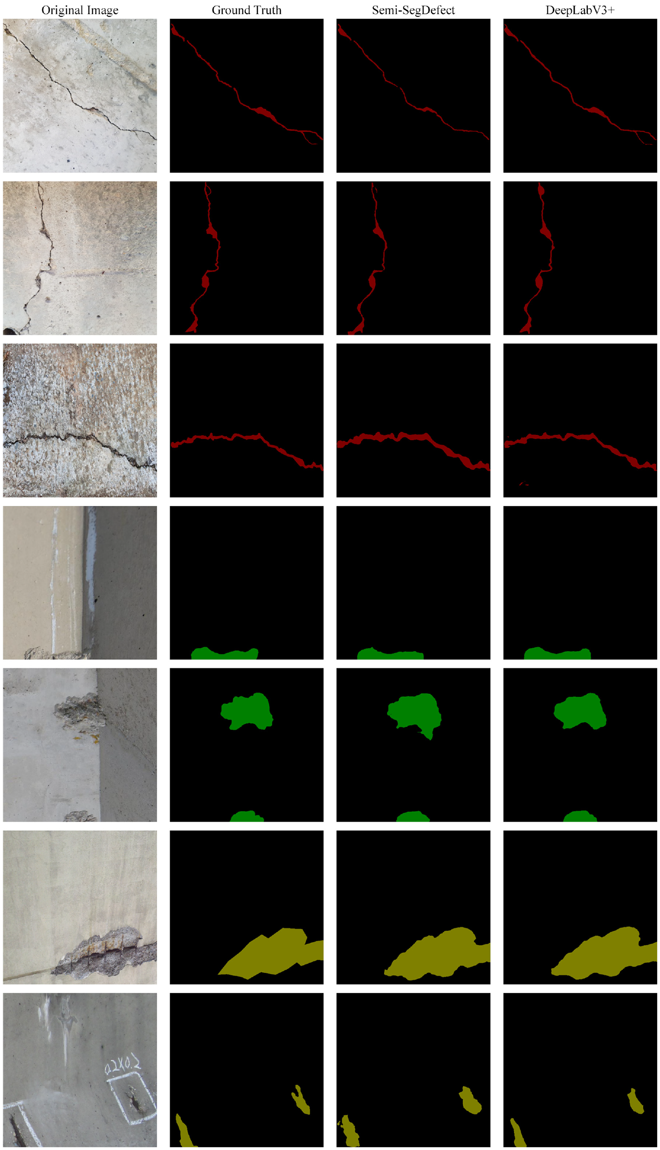
Samples of segmentation results.
Robustness test
Comprehensive robustness testing is paramount to assess the model’s capacity to perform effectively under various challenging conditions. These challenging images were instrumental in thoroughly evaluating the model’s performance and its ability to handle diverse and complex scenarios commonly encountered in concrete defect detection applications. We selected a set of images for model testing, some of which were captured in complex scenes, some exhibited coupled damages, and others contained interference factors such as damage-like edges/regions, variations in illumination, shadows, and motion blurs. Figures 9 and 10 depict the segmentation results of single and coupled defects by the model in complex scenarios, respectively. It can be seen that the proposed model has good adaptability to diverse and complex scenarios frequently encountered in concrete defect detection applications. Notably, the model demonstrates stronger generalization capabilities when it comes to identifying spalling and rebar exposure. This is primarily attributed to the pronounced characteristics of these two defect types, where the model adeptly captures the relevant distinctive features and patterns. In comparison, when it comes to detecting cracks, the model is prone to false negatives or false positives, particularly in scenarios with pronounced interference factors. These findings will motivate ongoing research and improvements to enhance the model’s capabilities for real-world applications.
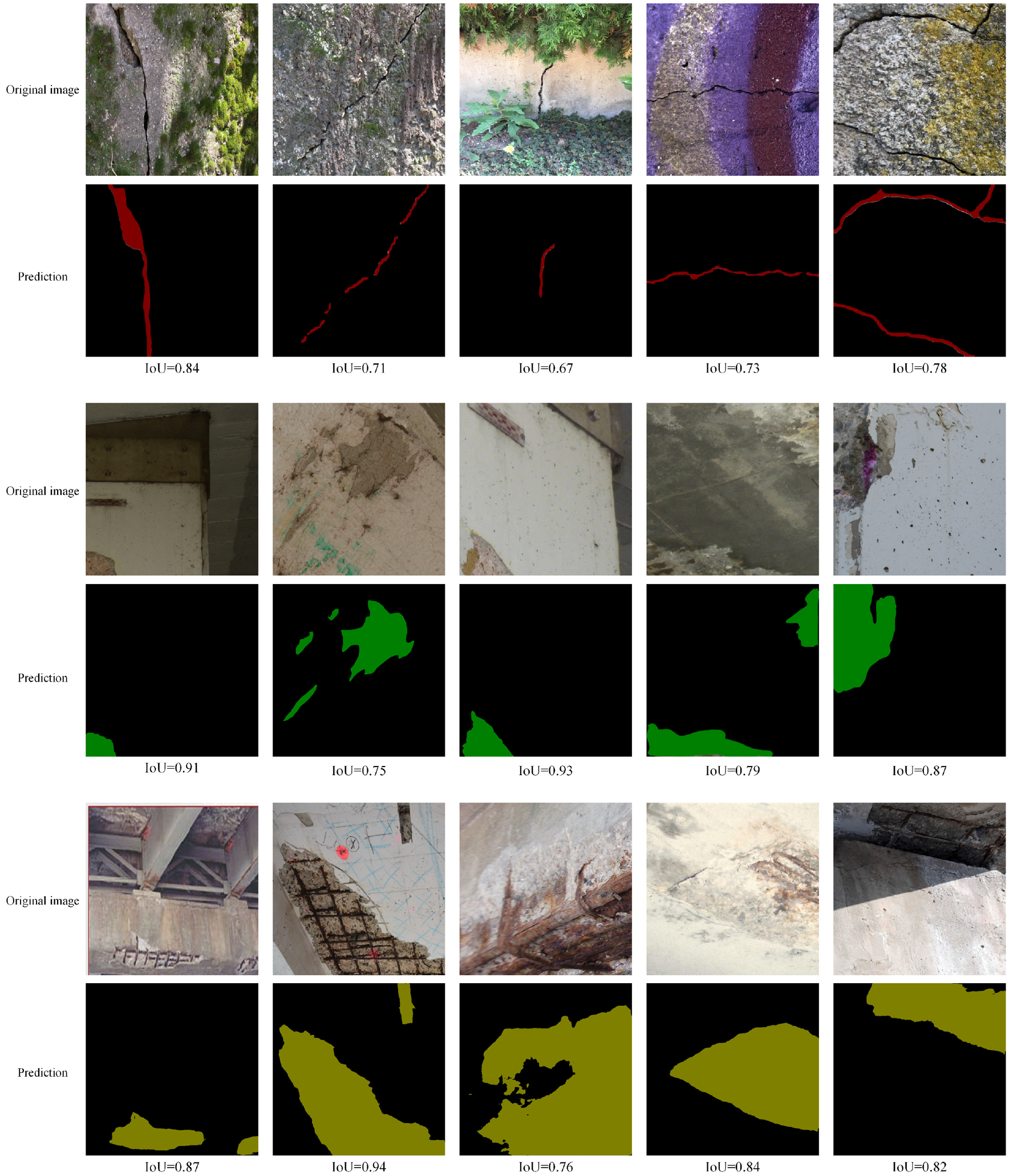
Samples of single defect segmentation results.
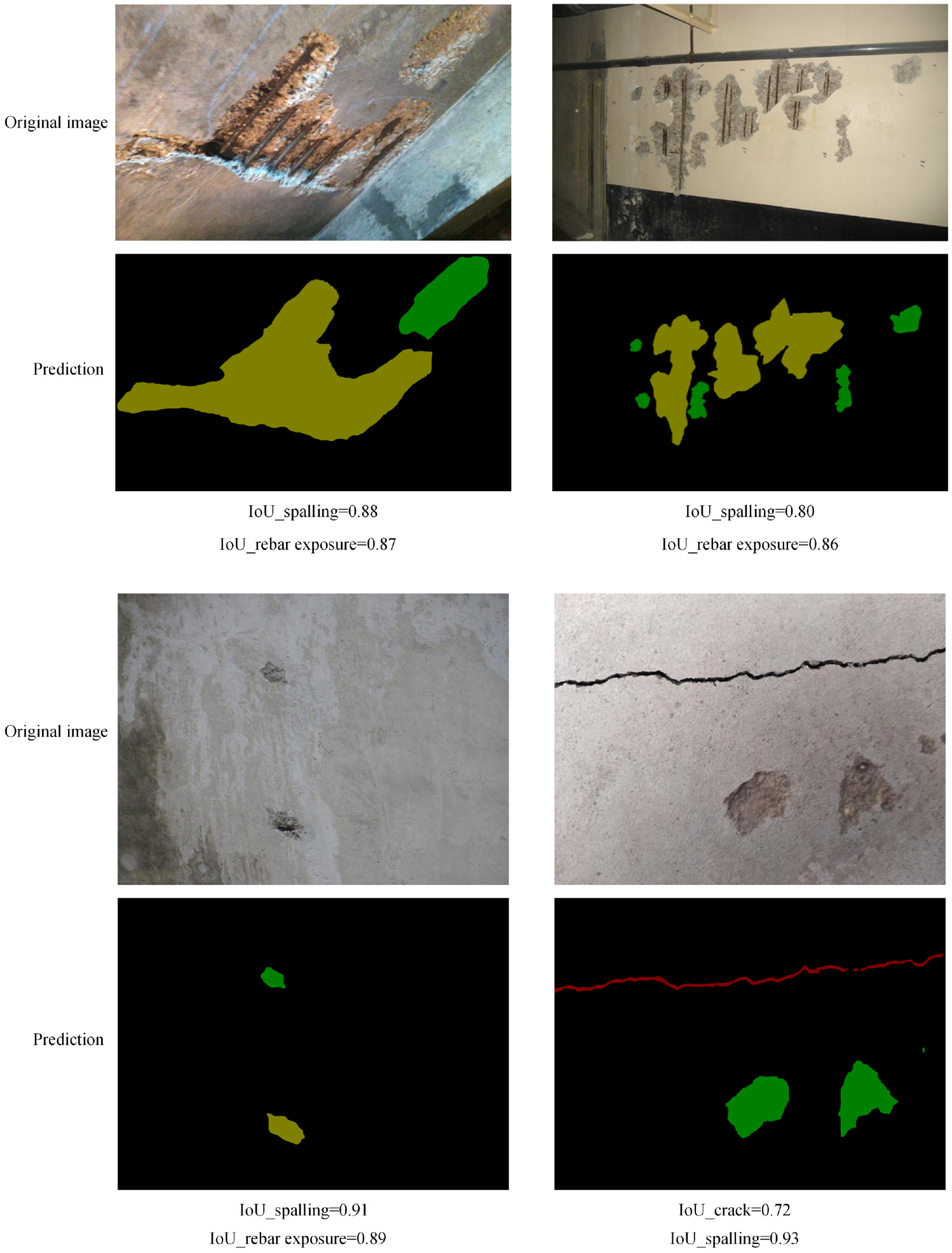
Samples of coupled defect segmentation results.
Visualization of the model decision process
In semi-supervised segmentation, the encoder is a critical component for extracting significant features from both labeled and unlabeled data. Leveraging the knowledge obtained from a vast amount of unlabeled data, the encoder can extract more robust features that are generalizable to new, unseen data. To gain insight into which features Semi-SegDefect uses to make predictions during the inference phase, and to determine whether the model focuses on the correct regions of the image, we utilized gradient-weighted class activation mapping (Grad-CAM) to visualize the encoder. The Grad-CAM algorithm operates by calculating the gradients of the predicted class score relative to the feature maps of the last convolutional layer in the encoder. These gradients are utilized to assign weights to the feature maps, producing a coarse localization map that indicates the regions of the image that contributed the most to the decision. The visualization results of Grad-CAM are shown in Figure 11, demonstrating that the encoder can activate the complete object of interest region while suppressing the irrelevant background region for concrete defect feature extraction, resulting in reliable predictions. The response areas in various scenarios are relatively concentrated, accurately capturing semantically related areas and focusing on important targets. This is crucial in concrete defect detection, as precise and dependable predictions are essential for ensuring the safety and structural integrity of concrete structures.
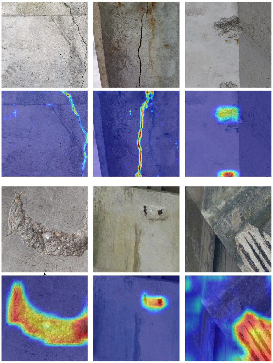
Visualization results of the encoder with Grad-CAM.
Discussion of semi-supervised and fully supervised learning
Semi-supervised learning and fully supervised learning are two approaches used to train models for image segmentation tasks. While both methods aim to improve the model’s accuracy in identifying objects within an image, they differ in the amount of labeled data required. Fully supervised learning requires a large amount of labeled data, which includes both the image and its corresponding ground truth segmentation masks, to train the model effectively. On the other hand, semi-supervised learning can achieve high performance even with a small amount of labeled data because it leverages a large amount of unlabeled data to improve performance. The model is trained using both the labeled data and the unlabeled data, where the unlabeled data are used to learn the underlying patterns and relationships in the data. By learning from both labeled and unlabeled data, the model can better understand the complex relationships within the data, resulting in better performance. The choice between semi-supervised and fully supervised learning depends on the availability of labeled data. If sufficient labeled data are available, fully supervised learning may be the better choice, as it has the potential to achieve higher performance. However, if labeled data are scarce, semi-supervised learning may be a more practical approach, as it can still achieve good performance with limited labeled data.
Conclusion
In this study, a semi-supervised segmentation model termed Semi-SegDefect was proposed to automatically perform pixel-level detection for concrete defects. Semi-SegDefect consists of a student model and a teacher model with the same structure. To achieve pixel-level contrastive learning, a decoder representation network is added in parallel with the decoder classification network, and the encoder output features are projected into a high-dimensional space to select anchor pixels and negative pixels. The hyperparameter selection and applicability study of the proposed Semi-SegDefect model was carried out on a public dataset of concrete defects. In view of the experimental study, several conclusions can be drawn:
The settings of learning rate, contrastive loss weight, and unsupervised loss weight play an important role in achieving better performance.
Most queries are redundant in pixel sampling space, and the activate sampling strategy is quite essential.
Sampling more anchor pixels and negative pixels means better model performance. After a certain point, the performance improvement becomes marginal, along with higher computational cost.
Semi-SegDefect can reach a higher MioU than a fully supervised segmentation model with a small number of labeled data. When using the 2%, 5%, 10%, and 20% training dataset, the MIoU reaches an improvement of 9.82%, 4.00%, 4.01%, and 3.69%, respectively.
Our proposal overcomes the dependence on large-scale labeled data, makes full use of unlabeled data to provide reliable supervision information for model training, and achieves the goal of improving model performance at a low cost. However, we chose to investigate the effects of each hyperparameter independently for efficiency and simplicity in this study. In future work, we will delve deeper into potential coupling influences and fine-tune hyperparameters for specific use cases. Furthermore, we plan to expand our dataset to include a wider range of defect types. This expansion will not only enrich the dataset but also contribute to a more comprehensive evaluation of our model’s performance across various real-world scenarios and structural conditions. In addition, the development of a structural health management platform will also be considered, benefiting from the advantages of deep learning and unmanned aerial vehicles to improve the efficiency of inspectors.
Footnotes
Declaration of conflicting interests
The author(s) declared no potential conflicts of interest with respect to the research, authorship, and/or publication of this article.
Funding
The author(s) disclosed receipt of the following financial support for the research, authorship, and/or publication of this article: The authors gratefully acknowledge the financial support of this research comes from the National Natural Science Foundation of China (grant no. 51579089).