
Abstract
Acoustic emission (AE) technology, as the main method of non-destructive testing technology, has been widely used in structural health monitoring (known as SHM) in the fields of machinery and civil engineering. Locating the failure source is an important application of SHM, and accurately identifying the moment when the AE signal first reaches the sensor (which is called onset time) is of vital importance. Deep learning model has been widely used in onset time determination of AE signals in recent years due to its powerful feature extraction ability. However, as one of the most popular models, Transformer has not been further studied in such field and its effectiveness remains to be proven. In this paper, a novel AE onset time determination method based on Transformer is proposed. Firstly, a preprocessing method based on segmentation-concatenation is applied to divide original data into several connected small segments, while the integrating labeling method is applied on small label segments. Secondly, the preprocessed data and labels are substituted into the Transformer model for training. Finally, for the sequence processed by the Transformer model, the first-time index that reaches the maximum value is obtained as the determination result. Based on the Hsu-Nielson source AE data, the feasibility and performance of this method are analyzed and compared with several commonly used methods: Akaike information criterion (AIC), short/long term average combined with AIC (STA/LTA-AIC), floating threshold (FT) and 1D-CNN-AIC method. The results show that the proposed method is significantly better than AIC, STA/LTA-AIC and FT. Moreover, the determination efficiency is greatly improved while the performance of the proposed method is close to that of 1D-CNN-AIC. Meanwhile, the method has robust performance especially in low signal-to-noise ratio scenario. In practical applications with small-scale data, the proposed method is of relatively high reference as well as application value.
Introduction
Acoustic emission (AE) is a common physical phenomenon in which the energy is generated by the local stress and released in the form of transient elastic wave rapidly. 1 The internal deformation, 2 crack propagation, 3 external impact friction 4 and other events will immediately generate and spread the AE signals, which are directly related to the structural failure mode, the location of the failure source and the degree of damage. 5 Appling AE signals as monitoring factor can quickly locate the internal failure and grasp the health status of materials and structures on time, which make it widely used in fields ranging from machinery 6 to structural health monitoring. 7
Several automatic onset-time picking methods have been proposed in recent years. Two types of the most classic onset time determination methods are the parametric determining methods represented by floating threshold (FT), 8 and auto-regression determining methods represented by Akaike information criterion (AIC) 9 and short/long term average The Short Term Averaging/Long Term Averaging (STA/LTA).10,11 Madarshahian et al. 8 applied four times of standard deviation value of noise segment as threshold to obtain the arrival time. Kim et al. 12 used single-stage and two-stage AIC method for onset time determination. Zhou et al. 13 proposed a hybrid algorithm including the windowing Lempel-Ziv complexity and AIC method combined with multi-scale theory to study arrival time identification. Earle and Shearer 14 used the AE signal and its first-order statistics to calculate the STA/LTA sequence and select the time-stamp at the largest change as the onset time. Chai et al. 15 used Shannon’s Entropy on the basis of the STA/LTA principle to divide the AE signal generated by the fatigue crack growth test of alloy steel into intervals, and calculated the probability distribution of each interval and the corresponding entropy value. The time point with the largest change is taken as the arrival time of the signal. The results show that in the case of low signal-to-noise ratios (SNRs), the picking accuracy of methods based on parametric analysis remains low, and methods based on autoregression need to rely on a reasonable sliding window length. The STA/LTA-based methods fail to accurately select the optimal arrival time from multiple moments with sharp changes. For large amount of waveform data, the computational and picking efficiency of these methods decreases with the increase of dataset, their picking accuracy and efficiency are not enough to meet the requirements. 16
Deep learning has a deep and optimized network structure, which can capture features and learn intrinsic connections with higher efficiency. Many scholars have tried to use deep learning algorithms to obtain accurate AE signal arrival times17,18 and extract the signal features.19,20 Zheng et al. 21 used a deep recurrent neural network (RNN) to identify the onset time of tiny seismic waves and AE signals. Guo et al. 22 used a deep Convolutional Neural Networks (CNN) network to classify each sampling point in the AE signal into noise and signal in advance, then used the labeled AE signal and its several high-order statistics as the input of the network. The sequence generated from network is then substituted into Nonlinear Curve Fitting and special density cluster analysis Density-Based Spatial Clustering of Applications with Noise (DBSCAN) to obtain the results. Zhu and Beroza 23 applied PhaseNet, an adjusted deep neural network, to facilitate one-dimensional micro-seismic data input to classify the P waves and S waves, and identify the boundary time point. Li et al. 24 used one-dimensional CNN network combined with AIC algorithm. The original waveform data is divided into small segments for model training, then the processed sequence from CNN model is substituted into AIC algorithm to find the time point with the lowest AIC value as the arrival time. Saad et al. 25 applied the Auto-encoder-like structure to denoise the seismic waveform data for time-of-arrival identification. The existence of background noise, however, makes the recognition accuracy of the deep learning network insufficient in the case of low SNR. The features required by the model are not generalizable for other waveforms with different data length, and the calculation complexity of models with CNN-like structure increases as the amount of data grows. The one-dimensional data, especially small-scale data, have not been fully utilized. The use of raw data needs to be more concise and direct.
The Transformer model has become one of the most popular deep learning frameworks in recent years due to its unique computing method. The main calculation module, known as Attention, 26 not only realizes the same calculation mode as RNN network does, but can also realize the parallel calculation strategy without using sequence alignment or considering the distance of the target segment in the input or output sequence.27,28 Moreover, compared with CNN, Transformer can keep the computational complexity at a certain level despite the increase of the input length. The Transformer network with stacked multiple Attention modules can realize the simultaneous parallel position calculation of the target sequence more efficiently. Recently, some scholars have begun to apply the Transformer network to the one-dimensional data prediction issue. Devlin et al. 29 proposed an improved Transformer-based BERT network to associate the target text with the context to achieve text data prediction. Lim et al. 30 added a recurrent layer and a gating layer to the Transformer network to realize the prediction of multi-input time series. Zhou et al. proposed an Informer network for long-series time series prediction problems. The new network can be smaller than its predecessor Transformer. The low time complexity and memory cost enable its ability for extremely long sequences identification work. 31 Transformer has been widely used in the fields of natural language processing and sequence prediction, but no scholars have applied it to the onset time determination of AE signals or P waves. By treating the AE signal as an encoded natural language sequence, and treating the data segments before and after the arrival time as interrelated expressions, it can provide a new solution for the onset time identification.
In this article, an AE onset time determination method based on Transformer is proposed. This method is composed of two main components. Unlike seismic signals, AE signals have to be collected at high sampling speed and the scale of datasets of AE events is usually smaller than seismic signals. Therefore, in the first part the original AE data is normalized and processed by preprocessing method based on segmentation-concatenation. The processed data is divided into small connected segments for feature extraction of Transformer model. To lower the calculation complexity and gain a better model performance, the integrating labeling method is applied to simplify the labels of processed data, where the status labels of all points in each segment are replaced by unique status value. The processed data and label values are then substituted into Transformer model due to its learning capacity among every data point. Original AE data is from Hsu-Nielson experiment carried out by Madarshahian, 32 the whole dataset contains different SNRs so the model can be trained under as many AE waveform circumstances as possible. The second part is the determination part. The ready-for-identification AE waveform is preprocessed by the same segmentation-concatenation strategy, then submitted into the trained Transformer model to generate the Transformer sequence. The index of the point that first reaches the maximum value of the Transformer sequence is determined as the result. Compared with traditional determination methods and some methods using deep learning for onset time identification, the proposed method directly uses the original AE data for calculation, training, and maximizes the use of training data. The performance of the proposed method is very robust within various SNR ranges, especially in low SNR range. The proposed method ensures the precision of the onset time picking of AE signals and improves the efficiency.
The main scientific contribution of this work is the development of an onset time determination method of small-scale AE datasets based on Transformer. To achieve this, a fixed-length sliding window is selected to divide the original data into small segments for concatenation, which can maximize the use of small-scale AE data and enable the model to be trained under a more realistic circumstance. The integrating labeling method, which is based on the 0,1 point labeling method, is proposed and applied to simplify the original status feature and calculation complexity. The first index of the Transformer sequence that reaches the maximum value is determined as the onset time. The experiment results show that the onset time of signals with various SNRs can be determined more accurately than with other methods. The proposed method uses data segments to represent the arrival time information of each data point and further optimization is made on this basis unlike other recognition methods using neural networks, which greatly reduces the cost of both training and recognition process, thus has the advantages of fast training speed and low computational complexity for small-scale AE signals. In addition, compared to the 1D-CNN-AIC method, 24 which has to use multiple features to generate convincing results, the method mentioned in this article applies data itself directly, which greatly simplifies the data preprocessing step, significantly reduces the determination time consumption and is more suitable for practical applications. Moreover, by treating AE signals as sequences of natural language and training the Transformer model, whose application in AE onset time identification has yet been relatively limited, on original data directly, the proposed method has achieved more robust results compared to several known classic identification methods without computing or adding other features. This expands the application of the Transformer model to the field of AE onset time identification, and its inherent parallel computing mechanism also reduces the computational cost of the recognition process. This method can be applied to determine the onset time of AE and micro-seismic signals, while in particular, it is believed to be used as a reference for the application of small-scale datasets as input to deep learning models.
The structure of the article is as follows. Section “Theory and background knowledge” describes the relative backgrounds of the determine method, including data preprocessing and Transformer model frameworks. The Hsu-Nielsen experiment (known as pencil lead break, PLB) AE data and the experiment details are described in section “Example”. Section “Performance and analysis” analyzes the method performance and results. Section “Discussions” describes the comparison of the proposed data and other traditional and deep-learning-based determining methods. Section “Conclusion” concludes this article.
Theory and background knowledge
Data preprocessing
The original AE data is normalized at first to avoid the bias effect caused by AE waveforms with different voltage value ranges. For a random AE sequence data
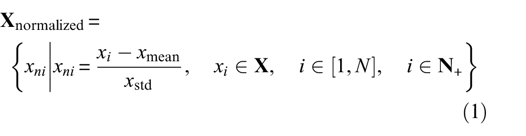
where
Since AE signals have to be collected at high sampling speed and the scale of datasets of AE events is usually smaller than seismic signals, to fully train the Transformer model, a segmentation-concatenation method is applied to the normalized sequences in order to maximize the use of data after the calculation process. Sequence in normalized data is first split with a fixed-length sliding time window with a length of l into several segments. As shown in Figure 1, a fixed-length time window slides on the data sequence to save the current selected segment and move to the next point to continue saving until the end. For a given normalized sequence
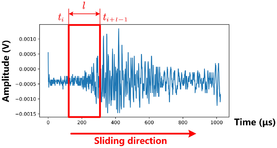
The example of segmentation.
The processing of data label values is equally important. Appropriate labeling strategy can reduce the computational complexity and improve the learning effect and overall performance of the model. It should be noted that in fields where AE-like data is needed, such as SHM, the onset time of signal is recorded as reference by experienced researchers through eye inspection, which is the ground truth.
The AE signal data used in this article comes from the interval sampling mode, with a sampling length of 1024. When the signal strength exceeds the preset threshold, the interval sampling is triggered, collecting the fixed-length signal segment from forward toward backward at the threshold point, where the forward sampling length is the pre-sampling length. Due to the environmental noise and other factors, the threshold-based method cannot accurately indicate the arrival time of AE event. The actual AE arrival time and the arrival time captured by the threshold-based sampling method on the data acquisition system do not occur at the same position. The distribution of the threshold-based sampling point and the actual arrival time sampling point is illustrated in the following Figure 2.
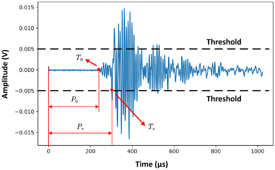
The illustration figure of the actual arrival time point and threshold-based sampling point, where
By taking the difference between the extracted AE arrival sampling point and the threshold-based arrival time sampling point, and knowing the sampling frequency, the precise arrival time can be easily calculated:
The signals collected in Madarshahian’s PLB experiment contain different SNRs. The method mentioned above can’t be applied to the signals with low SNRs. Thus, the equation can be modified. Since the sensor positions remain unchanged, the time difference between arrival of the PLB signal at any two sensors is fixed, and the wave velocity fluctuates merely over this propagation distance so it can be seen as a constant value, the Equation (2) can be adjusted as follows:
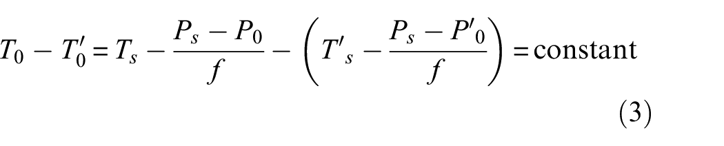
where
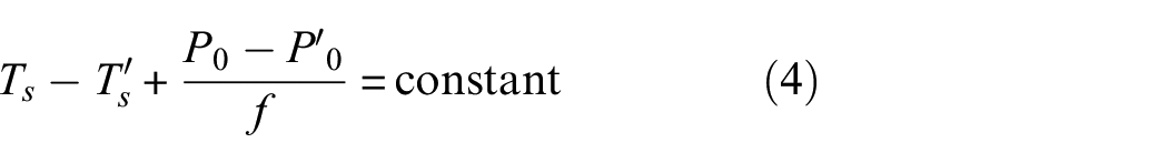
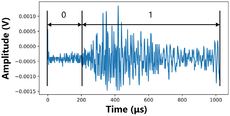
For the original AE data, as shown in Figure 3, the arrival status of each point is first marked manually, with 0 indicating that the point has not “arrived,” and 1 indicating that the point has “arrived.” When the labeling is completed, the label value is further processed by the integrating labeling method. In order to correspond to the AE signal data after segmentation-concatenation, the sum of the labels of each point in each segment is used as the basis for the integration judgment. When the summed value meets the specified threshold for small segments, the status of the entire segment is represented by 1, and the unsatisfied segment is represented by 0. The purpose of this labeling strategy is to replace the state label of each point with the overall 0, 1 state label.
Manual labeling of original acoustic emission waveform data.
For a given label sequence
where
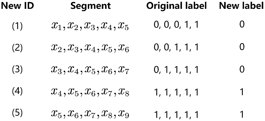
The layout of an example of integrating labeling strategy (threshold of label is set to 1).
Structure and training process of Transformer model
Attention and Transformer
The Transformer structure in this article is applied as deep learning framework due to its unique and powerful parallel calculation. As shown in Figure 5, the Transformer network consists of encoder structure formed by multiple stacked Multi-head attention blocks. The decoder part is not applied because the determination process is digitally related and there is no need for conversion between numbers to text. The positional encoding, Multi-head attention, and residual connection, layer normalization combined with feed forward, are three main parts to realize the calculation which are shown in section “Main calculation procedure in Transformer” in detail.
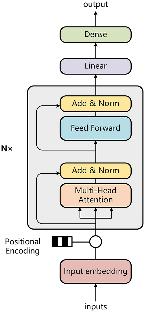
The schematic diagram of the typical encoder structure of Transformer model.
Main calculation procedure in Transformer
Positional encoding
The natural language characters cannot be directly recognized by computers. Characters need to be converted into digital codes before they can be input into the encoder for conversion. The function of positional encoding is to combine each character with positional embedded elements to generate the corresponding digital expression, the dimensions of the expression can be expressed as Equation (6):

Where
For data with nothing but pure digital components, such as AE signals, the positional encoding process can be ignored because the data value of each point can be regarded as its unique character. In order to ensure that Multi-head attention can recognize the input digital data, the dimension of the input needs to be adjusted, where
Multi-head attention
After expanding the dimension of the input sequence to

In order to facilitate the following calculations, the dimension is transposed into Equation (8):

It should be noted that for one-dimensional signal data, the dimension value of
Visual example of natural language processed by Attention calculation. Regions with brighter colors are more strongly correlated.
For one set of weight matrices

Where
Multi-head attention is based on the above single-head attention. Multiple concatenated attention heads are multiplied with the initial weight matrix
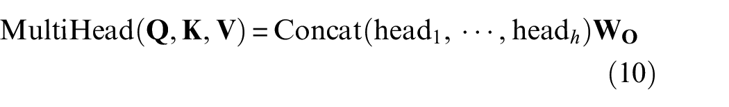
where
Residual connection, layer normalization and feed forward
Layer normalization is to speed up the training speed and accelerate the convergence. The formula can be expressed as Equation (11):

where m represents the number of rows of the matrix in the hidden layer,
Each layer of the encoder structure in the Transformer model contains a fully connected Feed forward network (FFN) to receive the output from Attention module. FFN consists of two linear transformations, which are activated by the ReLU function:

where
Integrating labeling strategy
As can be seen from the previous section, Transformer’s learning method is to calculate the distance between each point in the sequence and other points (including itself), that is, not only to calculate the data point multiplication and status point multiplication of each two data points, but also to calculate the relationship between data and status. Although the computational complexity of Transformer does not increase with the increase of sequence length, which is much better than RNN and CNN, the Transformer model will still face massive computational costs, and even the problem of memory overflow will appear during training if the original per-point status labeling strategy is used. After considering the computing characteristics of Transformer, the integrating labeling strategy is proposed and applied to greatly reduce the computational complexity and memory usage, and also ensure that the arrival information will not be lost, because the label of the entire segment will become 1 only when the sum of the labels satisfies the condition.
Another important issue is why the threshold is multiplied in the Equation (5). When the threshold is 1, that is, the sum of the label of each point in small segment is equal to the window length, so that the status label of the entire small segment is 1. It seems that the arrival time information of the manually labeling is perfectly preserved, which has little effect on signals with high SNR, but there is a significant hysteresis influence for low SNR signals. There is no difference in signals with high SNR whether the sum label value in a small segment is 1 (but at least more than 0.5), because the amplitude difference between the signal segment and the noise segment can make this effect almost negligible. However, in a signal with low SNR, such as shown in Figure 3, the state of the point corresponding to the small segment is already at the onset status when the label value of each point is not all 1 (the proportion of the label 1 is probably 0.7 or 0.8). Therefore, in order to improve the model performance and determination precision, by setting a threshold less than 1 in Equation (5) and lowering the onset standard, the characteristics of Transformer calculation and low SNR data can be better balanced as much as possible.
Algorithm workflow
The workflow of the proposed method is shown in Figure 7. Figure 7(a) is the first part of the method, the Transformer model training part. In this part, original AE data is substituted into the Transformer model for training after the data preprocessing part, and the model is saved when the training is completed. Figure 7(b) is the second part of the method. The data that needs to be recognized is substituted into the saved model, and the first-time index with the maximum value in the processed Transformer sequence is obtained as the arrival time. The specific content will be explained in the next few subsections.

The overall layout of the proposed method: (a) Transformer model training process and (b) onset time determination process.
Example
Experiment and data
The PLB experiment is also called Hsu-Nielsen experiment; 33 it simulates the generation of AE sources by breaking the pencil lead on the solid surface. The PLB experiment is easy to implement and the steps are simple, which is convenient for the arrangement and reception of sensors. The signals generated are different at each time, and the data is highly processable for neural network training, so that the training effect of the model will be guaranteed.
Based on Hsu-Nielsen’s research in the 1970s, Madarshahian replicated the PLB experiment in the laboratory and made the collected AE data public. Due to the instantaneity and unpredictability of AE sources, acquiring sufficient AE signal data is difficult in real engineering applications. The common practice in the field is to use PLB tests to simulate faults, thereby repeatedly acquiring large amounts of AE signals. The AE fault signals generated by such PLB simulations have a similar distribution to those generated by instantaneous faults in engineering practice. Whatsoever, the components in most AE signals of researchers’ interest are in the high frequency range, methods like filtering and denoising can be applied to process these AE signals, and thus the processed AE signals can be obtained which are similar to the ones under laboratory conditions. Therefore, using PLB tests to simulate faults is feasible. The PLB test is a standard test in the field of civil engineering, with rigorous procedure and clear generated AE event data, which is convenient for analysis and processing. Some researchers have used this data set to conduct time-of-arrival identification research. Yang et al. used this dataset to identify the time of arrival by applying the histogram distance method 34 and hybrid method combined with AIC. 35 Madarshahian et al. 36 proposed an autonomous inverse Bayesian-based source localization model framework by using this dataset to choose the most accurate onset time among several picking methods.
As shown in Figure 8, 10 piezoelectric AE sensors are placed on four surfaces of the concrete block: upper, lower, front and rear. Before placing the sensor, the contact surface between the sensor and the concrete sample is kept clean and smooth to ensure that the AE signal is not disturbed by additional noise such as voids and dust. Epoxy resin coupling agent was used to fix between the sensors and the surfaces of the sample respectively. The model of these sensors is PK WDI produced by MISTRAS with an operating frequency range of 200–850 kHz, and their built-in low-power amplifiers gain is set to 26 dB. A 24-channel Express-8 data acquisition system manufactured by MISTRAS Group was connected to the sensors to collect detected AE signals with a sampling frequency of 1 MHz, and overall threshold is set to 31 dB. Peak definition time, hit definition time, hit lockout time (HLT), and pre-trigger time were set to 200, 400, 200, and 256 μs, respectively.
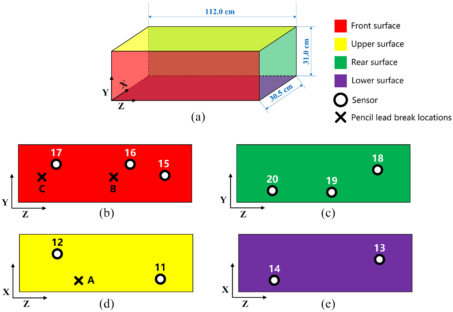
Concrete sample layout and positions of sensors as well as pencil lead break 24 : (a) Schematic diagram of concrete sample structure, (b) front view of sample, (c) rear view of sample, (d) upper view of sample and (e) lower view of sample.
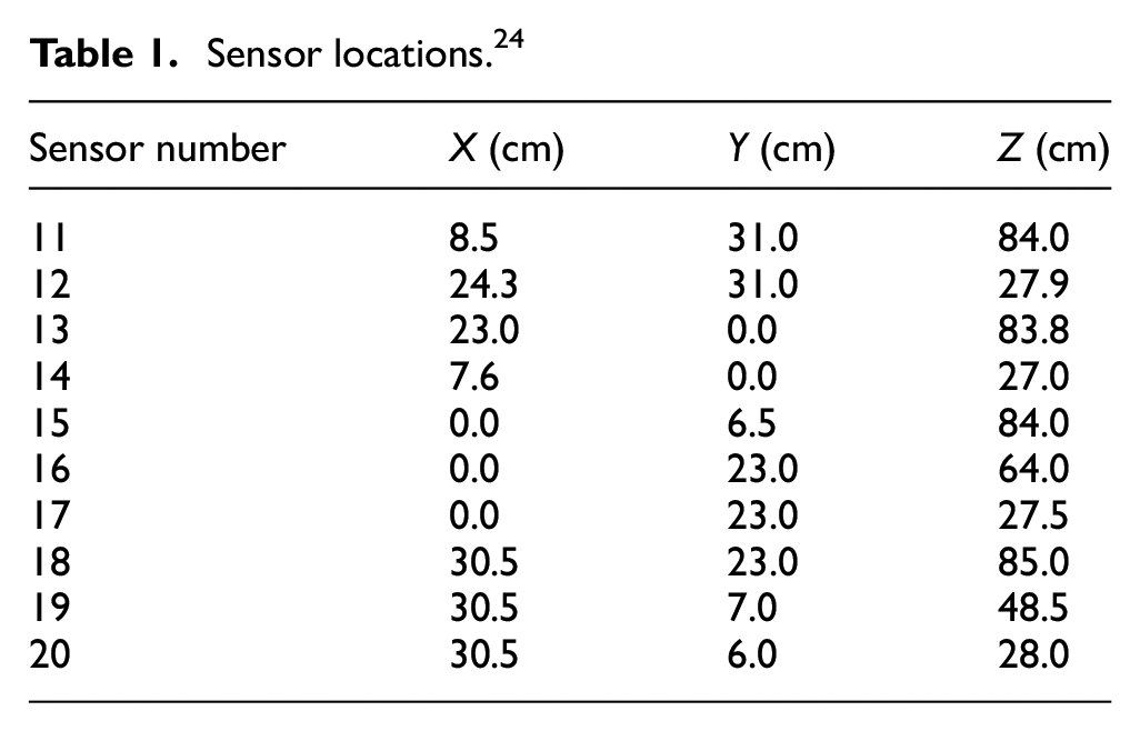
After the experimental devices are set, the pencil lead with a hardness of HB and a diameter of 0.3 mm is broken manually at three positions namely A, B and C on the surface of the concrete sample, and the generated stress wave propagates to the piezoelectric sensors. During this period, the stress waves are converted into electrical signals by the data acquisition system, amplified by the built-in amplifier, and uploaded to the computer. The collected data is divided into three groups: group A, B and C, where A is for model training and B, C are for validation. Each of group A and B contains 100 pieces of records while group C contains 99 pieces, a total of 299 pieces of data. All pieces of data is of the same length, with 1024 points, and the interval between two adjacent points is 10−6 s (1 μs), which is the system sampling interval. The ordinate is volts (V) representing the voltage value at each point. The number of sensors and spatial location information are shown in Table 1, and the coordinates of the PLB are shown in Table 2.
Sensor locations. 24
PLB locations. 24
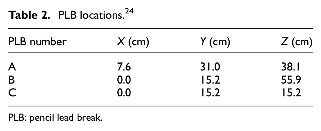
PLB: pencil lead break.
Data preprocessing
The PLB experiment generated three groups of signal data, named A, B, and C respectively. Group A and B had 100 waveform records while group C had 99 waveform records. Each record contains an AE event with a length of 1024 points (1024 μs). The arrival times of all events, that is, the label values, are manually annotated. It should be noted that in fields such as materials and geology that utilize AE technology, the arrival time of the AE signal is judged and recorded manually by experienced researchers, which is proprietary to the field. For the Transformer network mentioned in this paper, the manually calibrated arrival times are more meaningful for training. Before using these data, the arrival time of all data is manually discriminated and recorded.
Group A data is selected as training data and standard normalization is applied. In order to generate a data set that can be fully trained in Transformer with appropriate dimensions, the length of the moving window l is set to 128, and each waveform trace can generate 897 segments, so the entire training data can generate a total of 100 × 897 segments. Each segment is a matrix with dimension of (128, 1). The dimension of the overall data matrix
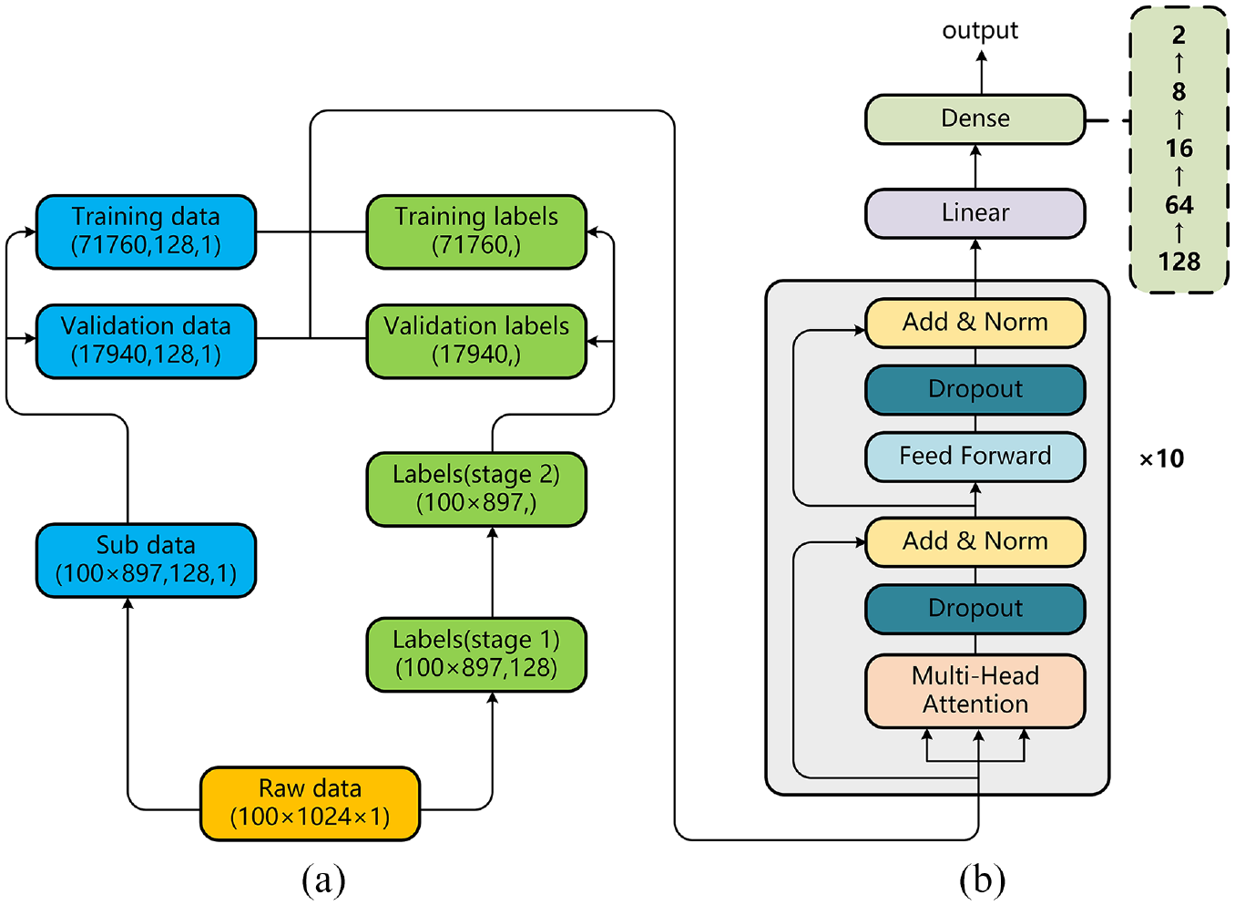
Layout of data preprocessing and model structure: (a) data preprocessing part and corresponding dimensions and (b) model structure.
Figure 9(b) is the structural part of the Transformer model. Multi-head attention, residual connection and layer normalization, feed forward network and dropout layer are combined together as a basic module. The 10-layer basic module blocks are stacked and gradually decreases with the 5-layer dimension. The entire Transformer model structure consists of 10 stacked basic modules and five layers of fully connection layer with dimensions decreasing layer by layer. The preprocessed data is substituted into the Transformer model, and the final probability value is generated after multiple iterations of training. Dropout 37 and global pooling average strategy are applied in order to make the model fully understand the nonlinear features and enhance the performance. The hyperparameters of the model are shown in Table 3.
Hyperparameter settings of Transformer model.
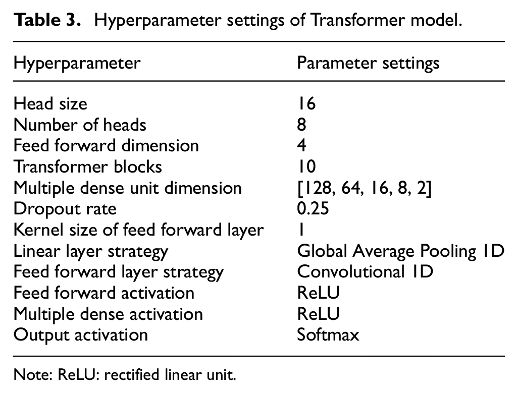
Note: ReLU: rectified linear unit.
The data of groups B and C are used as test data. The dimension of the data to be identified needs to be converted to be the same as that of the training dataset through the segmentation-concatenation method. Each segment in the processed matrix is substituted into the model to generate corresponding values, forming a sequence with values between 0 and 1. For the generated sequence, the first-time coordinate of the point where it reaches the maximum value is obtained as the identified arrival time.
Performance and analysis
Overall performance
The loss function score and Sparse Categorical Crossentropy (SCC) function score of the Transformer model during training are shown in Figure 10. The Transformer model uses 20% of the input data as the validation set during the training process, allowing the model to optimize parameters through the validation set after each iteration. It can be seen that the loss value of the training set gradually decreased to 0.044, the SCC score increased rapidly after the 35th iteration, and the growth trend slowed down and converged to 0.982 after the 73rd iteration. The loss and SCC scores of the validation set converged to 0.032 respectively and 0.986 respectively. In order to comprehensively demonstrate the performance of the entire model, distribution analysis was performed on the identification results of the data in group B and C.
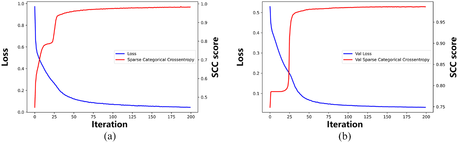
Loss and SCC score of Transformer model: (a) the loss and SCC score curve of the training set and (b) the loss and SCC score curve of the validation set.
The performance distribution of group B and C is shown in Figures 11 and 12, respectively. It can be seen from Figure 11(a) that the difference between the identification results and the manual identification is concentrated between −20 and 40 μs. It is more obvious in Figure 11(b), where the data with absolute difference within 20 μs accounts for 47%, and the data within 40 μs accounts for 94%. The distribution of group C is shown in Figure 12. Similar to group B, the difference distribution of the results is mostly concentrated within −50 to 50 μs, of which the absolute difference within 20 μs accounts for 54%, and within 50 μs accounts for 94%.
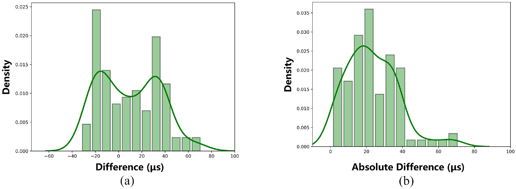
Histogram and density curve of difference distribution of group B: (a) Histogram and density curve of difference distribution and (b) Histogram and density curve of absolute difference distribution.
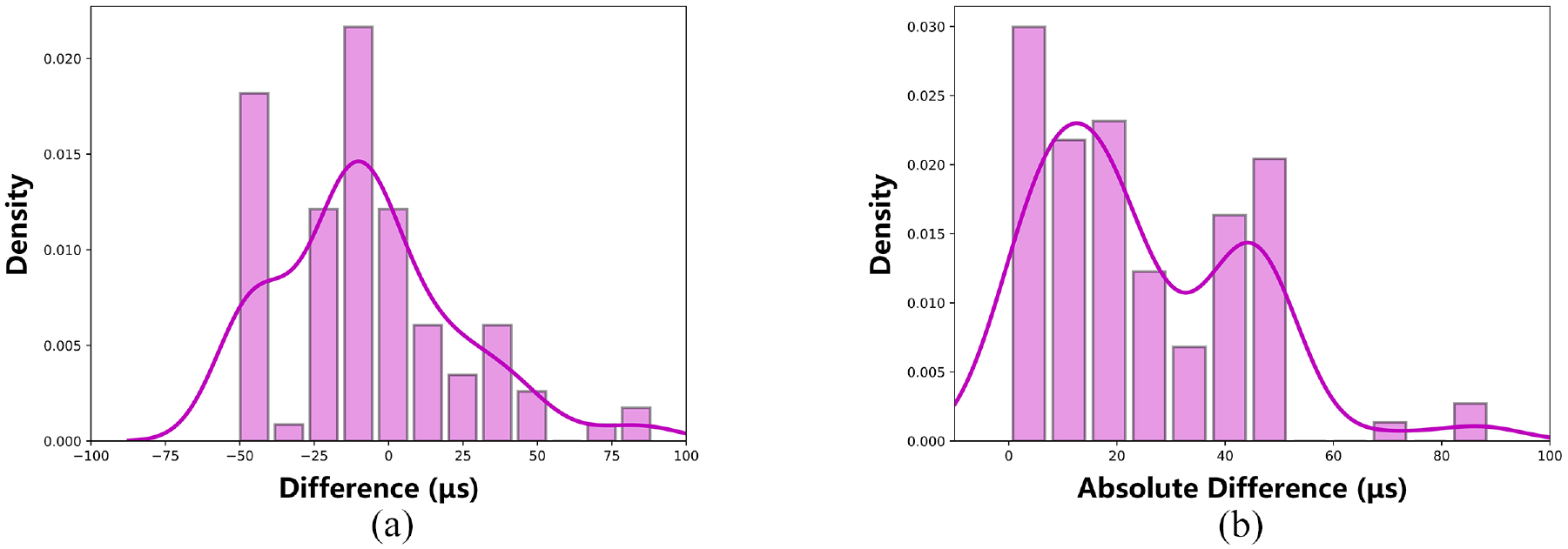
Histogram and density curve of difference distribution of group B: (a) Histogram and density curve of difference distribution and (b) Histogram and density curve of absolute difference distribution.
Low SNR performance
In order to analyze the performance of the Transformer-based determination method in each SNR interval, the absolute difference between the results of group B and group C is classified according to the SNR interval, and the scatter plot and corresponding box plot of the distribution are shown in Figures 13 and 14. The abscissa is the SNR interval, which is divided into four parts: <0, 0–1, 1–5, 5–10, >10. Figure 13 is the layout of distribution of group B, and Figure 14 is the layout of distribution of group C. It can be seen from the figures that in the first three lower SNR intervals, the main distributions of groups B and C remain within 40 μs. In the medium-high SNR interval, the main distributions of groups B and C remain within 40 and 50 μs respectively. It shows that the Transformer method is more reliable in the middle and high SNR range.
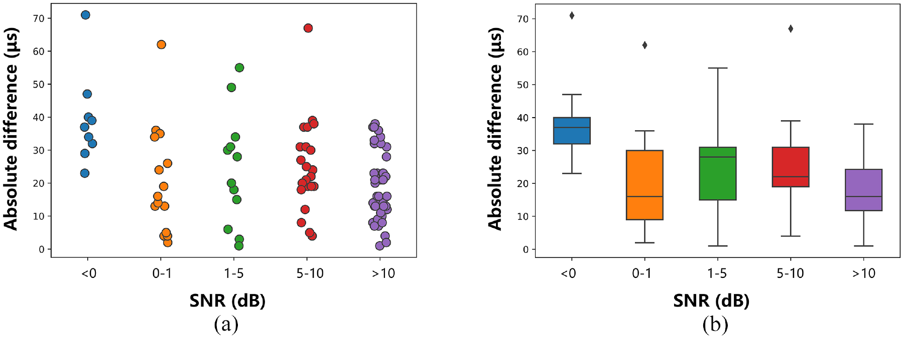
Scatter plot and boxplot of absolute difference at each SNR interval in group B.
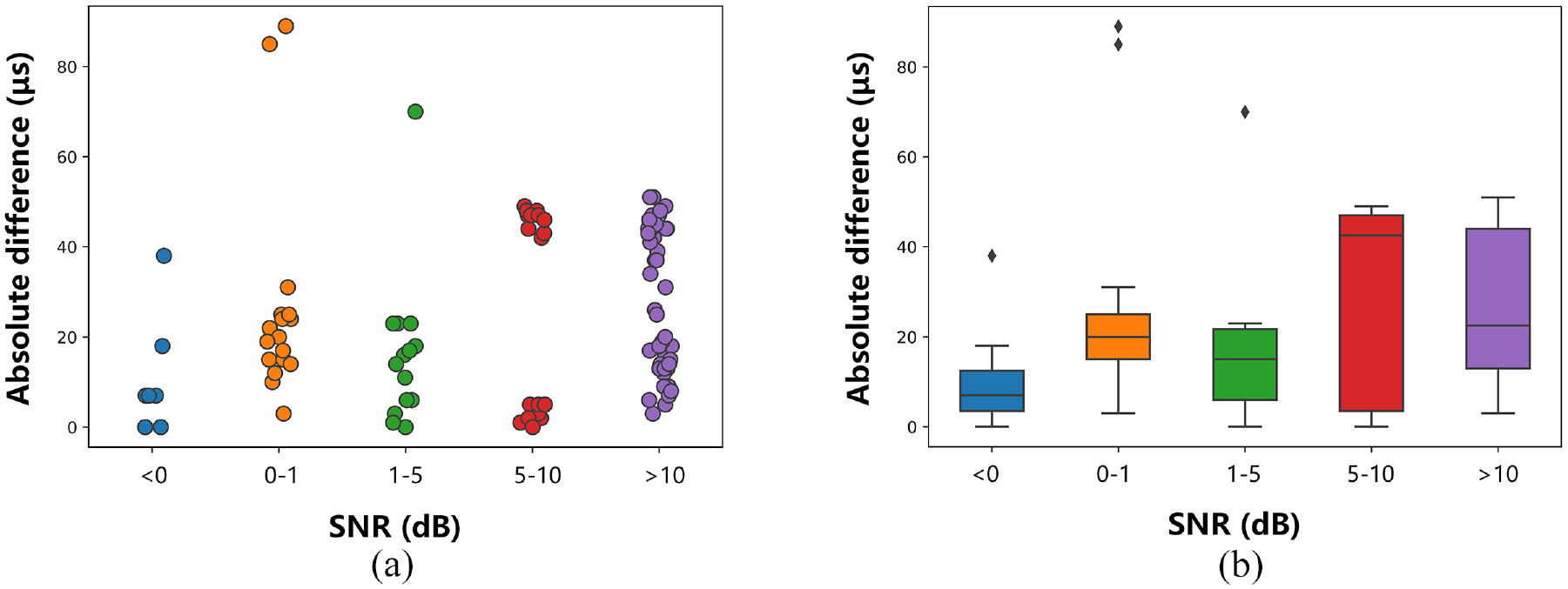
Scatter plot and boxplot of absolute difference at each SNR interval in group C.
Figure 15 shows the joint distribution diagram of the absolute difference of the determination results of group B and group C in each SNR interval, where (a) is the distribution of group B and (b) is the distribution of group C. The darker the contour area, the more concentrated the distribution. The curves at the top and right of the figures represent the corresponding density variation curves of SNR and absolute difference, respectively. The higher the curve, the higher the frequency of the region. It can be clearly seen from the figure that the data volume of the low SNR and high SNR data of group B and C is similar, and their identification results are mainly distributed within 40 and 50 μs. The performance of this method is relatively robust in each SNR interval.
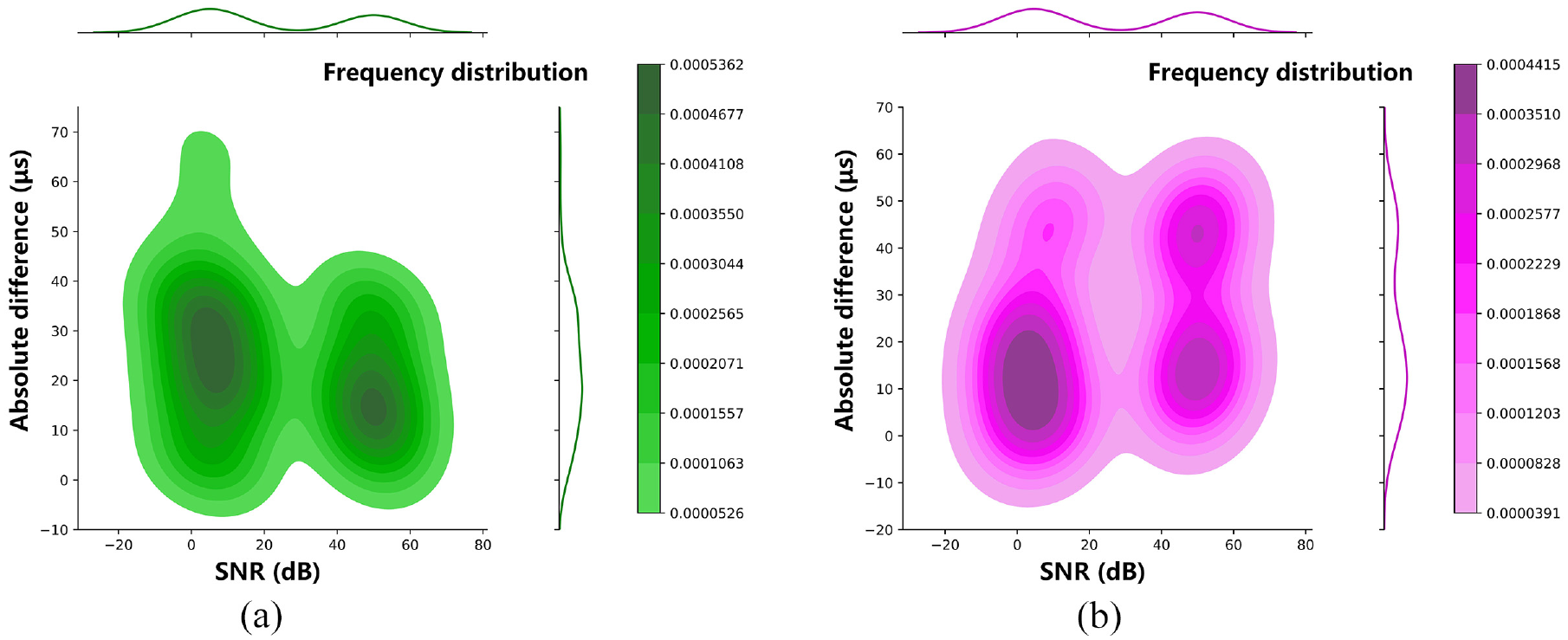
The joint distribution diagram of the absolute difference in each SNR interval: (a) the joint diagram of group B and (b) the joint diagram of group C.
Two pieces of data with low SNR characteristics in group B and group C are respectively selected as examples. The prediction results are shown in Figure 16(a) and (b). From top to bottom are the original waveform, the Transformer processing sequence, and the original waveform with the final determination result and manual recognition marks. The green dotted line represents the final recognition arrival time of the model, and the red solid line represents the arrival time of manual recognition. It can be seen from the figure that for the waveform signal with low SNR, the arrival time identified by this method is relatively close to that of manual identification, which further shows that this method has a certain robustness especially for low SNR waveform identification.

Performance examples of waveforms with low SNR: (a) Waveform ID: PLB B_11_8918128 and (b) Waveform ID: PLB C_11_39457496.
Discussions
Background knowledge of AIC, STA/LTA and FT
To better illustrate the performance and reliability of the proposed method, AIC, FT, STA/LTA-AIC method, and the 1D-CNN-AIC method which is proposed by authors previously, are also applied to groups B and C.
The essence of AIC, built on the concept of information entropy, is an autoregressive estimation of a given series of statistical data as a measure of the complexity and superiority of a model cluster.38,39 In sequences containing multiple distinct events, this criterion can effectively separate the different events in the sequence. Akaike showed that a time series can be divided into two or more locally stationary segments, where the interval before and after the arrival time can be assumed to be two time series with different statistical characteristics. 40 The moment of the minimum point in the time series processed by the AIC algorithm is the separation point of the two time periods, that is, the arrival time. 9 The commonly used AIC calculation method is the improved version proposed by Maeda on the basis of Akaike. 41
For a random AE sequence data
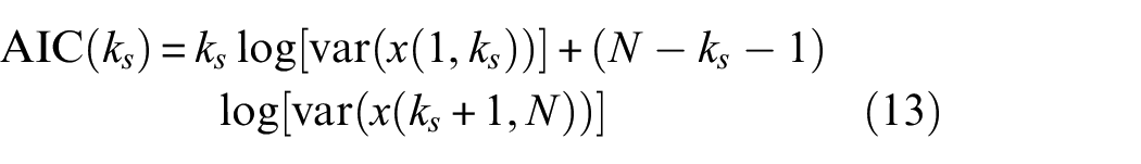
where
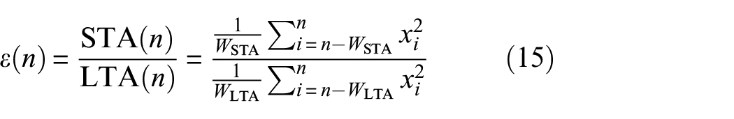
STA/LTA is defined as the ratio of the short-term average to the long-term average of time series data, and is the most widely used algorithm in automatic P-wave detection in the field of seismic signal processing. 5 The STA/LTA method assumes that when an arrival event occurs, the STA increases much faster than the LTA, so the onset time can be determined by setting a threshold for the STA/LTA series. 42 The algorithm has two moving windows, namely the STA window and the LTA window, and the formula is expressed as Equation (14):
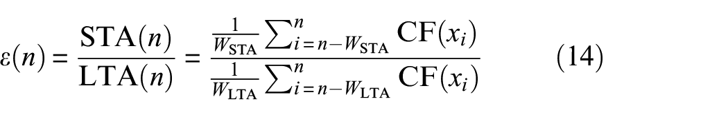
where
In order to optimize the automatic identification process, STA/LTA can also be combined with AIC as the onset time identification method, that is, AIC is used to identify the sequences generated after STA/LTA processing. Moreover, AIC can also be combined with some deep learning networks. The 1D-CNN-AIC method, which is proposed by the authors for example, uses the AIC algorithm as the final decision step of the 1D-CNN model. 24
The FT method assumes that the environmental noise is a stationary signal, while the AE signal is a sudden change signal. When the signal amplitude changes greatly and exceeds the threshold, the index that first crosses the threshold is assumed as the arrival time. The threshold setting of the FT is based on noise, but the fixed threshold cannot be applied to other waveforms since the noise amplitude of each AE waveform is different. Therefore, the statistical characteristics of the local noise section of the current waveform are applied as the standard. The FT method is usually associated with a sliding time window. If the local feature value in the time window exceeds the set threshold, it is determined as the arrival time. 43
For a random AE sequence data
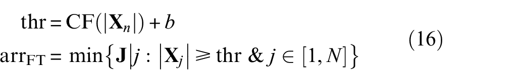
where
Comparison with AIC, STA/LTA-AIC, FT picking method
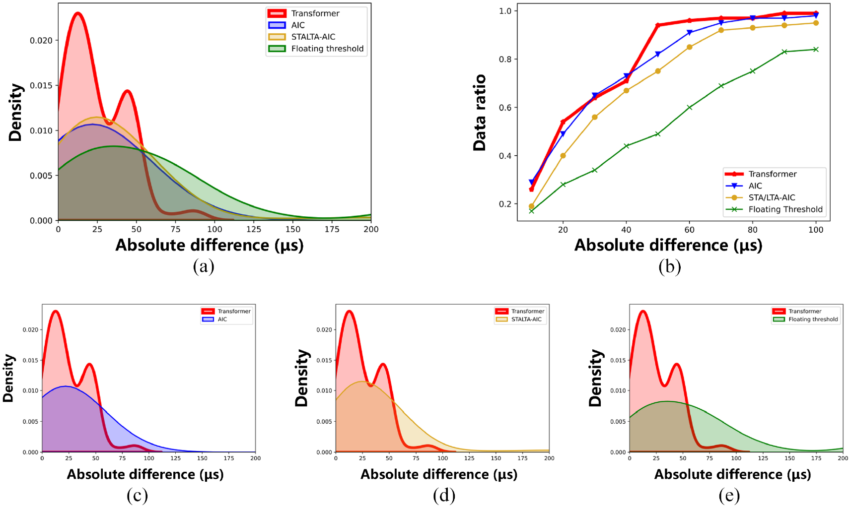
First, the results performance and distribution diagrams of the proposed method and the AIC, STA/LTA-AIC and FT methods of groups B and C are shown in Figures 17 and 18, respectively. The abscissa of the two figures is the absolute difference between the determination result and the manually picking result. In these two figures, the overall distribution density plots of the proposed method and the three methods are shown in (a), while (c), (d), (e) are the proposed method versus the three methods respectively. The red, blue, yellow and green curves and shaded areas represent the density distribution of the proposed method, AIC, STA/LTA-AIC and FT respectively. As can be seen from (c), (d) and (e), when dealing with the same data, the distribution of the proposed method is more concentrated than that of the other methods, mostly within 40 μs (group B) and 50 μs (group C). It is obvious from Figures 17(a) and 18(a) that the proposed method outperforms the other three methods.
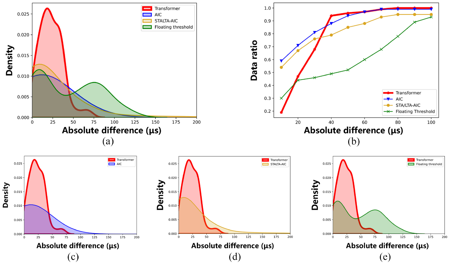
Difference distribution histogram and line chart of the proposed method, AIC, STA/LTA-AIC and FT on group B dataset. Red, blue, green and yellow solid polylines and density plots represent the proposed method, AIC, STA/LTA-AIC and FT respectively: (a) density plot of four methods, (b) distribution line chart of four methods, (c) density plot of proposed method versus AIC, (d) density plot of proposed method versus STA/LTA-AIC, and (e) density plot of proposed method versus FT.
Difference distribution histogram and line chart of the proposed method, AIC, STA/LTA-AIC and FT on group C dataset. Red, blue, green and yellow solid polylines and density plots represent the proposed method, AIC, STA/LTA-AIC and FT respectively: (a) density plot of four methods, (b) distribution line chart of four methods, (c) density plot of proposed method versus AIC, (d) density plot of proposed method versus STA/LTA-AIC and (e) density plot of proposed method versus FT.
In the polyline chart (Figure 17(b)), the proposed method seems to perform not as good as the other three methods within the 40 μs absolute difference interval, but after the 40 μs absolute difference interval, the proposed method is already close to 100% interval distribution. The rising trend of the other three methods is slower and the distribution of results is not as concentrated as the distribution of the proposed method, which can be seen more clearly in Figure 18(b). The performance of group C outperforms the other three methods significantly, reaching a 94% distribution within the first 50 μs absolute difference interval.
Comparison with 1D-CNN-AIC picking method
In authors’ previous work, 1D-CNN-AIC is proposed to be a robust determination method. It uses 1D-CNN to extract the various features calculated from AE data and uses AIC for final determination step. 24 As shown in Figure 19, the performance of the two methods is relatively close, and the results obtained by the 1D-CNN-AIC-based method are more concentrated than those obtained by the Transformer-based method. It can be seen from the (b) and (c) subplots that within each SNR interval, the results presented by the Transformer method are more divergent than that of 1D-CNN-AIC, and the determination precisions are mostly maintained at 40 μs (Figure 19(c)) and 50 μs (Figure 20(c)), which are inferior to 1D-CNN-AIC’s 40 μs (Figure 19(b)) and 30 μs (Figure 20(b)).
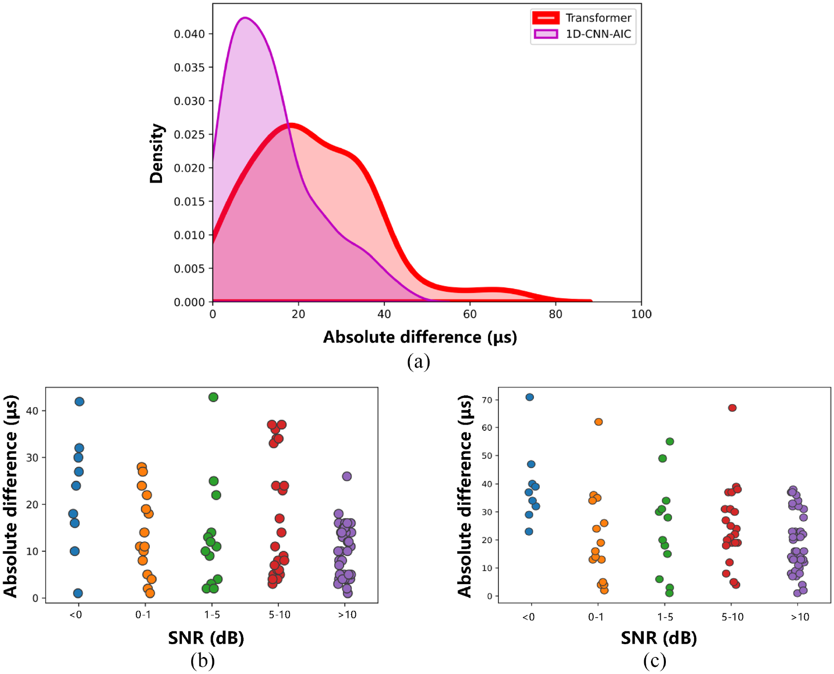
Density diagram and scatter plot of the proposed method and 1D-CNN-AIC method in group B: (a) density diagram of the two method, light green curve and region represent 1D-CNN-AIC and darker ones represent the proposed method, (b) the scatter plot of the 1D-CNN-AIC method at each SNR interval and (c) the scatter plot of the proposed method at each SNR interval.
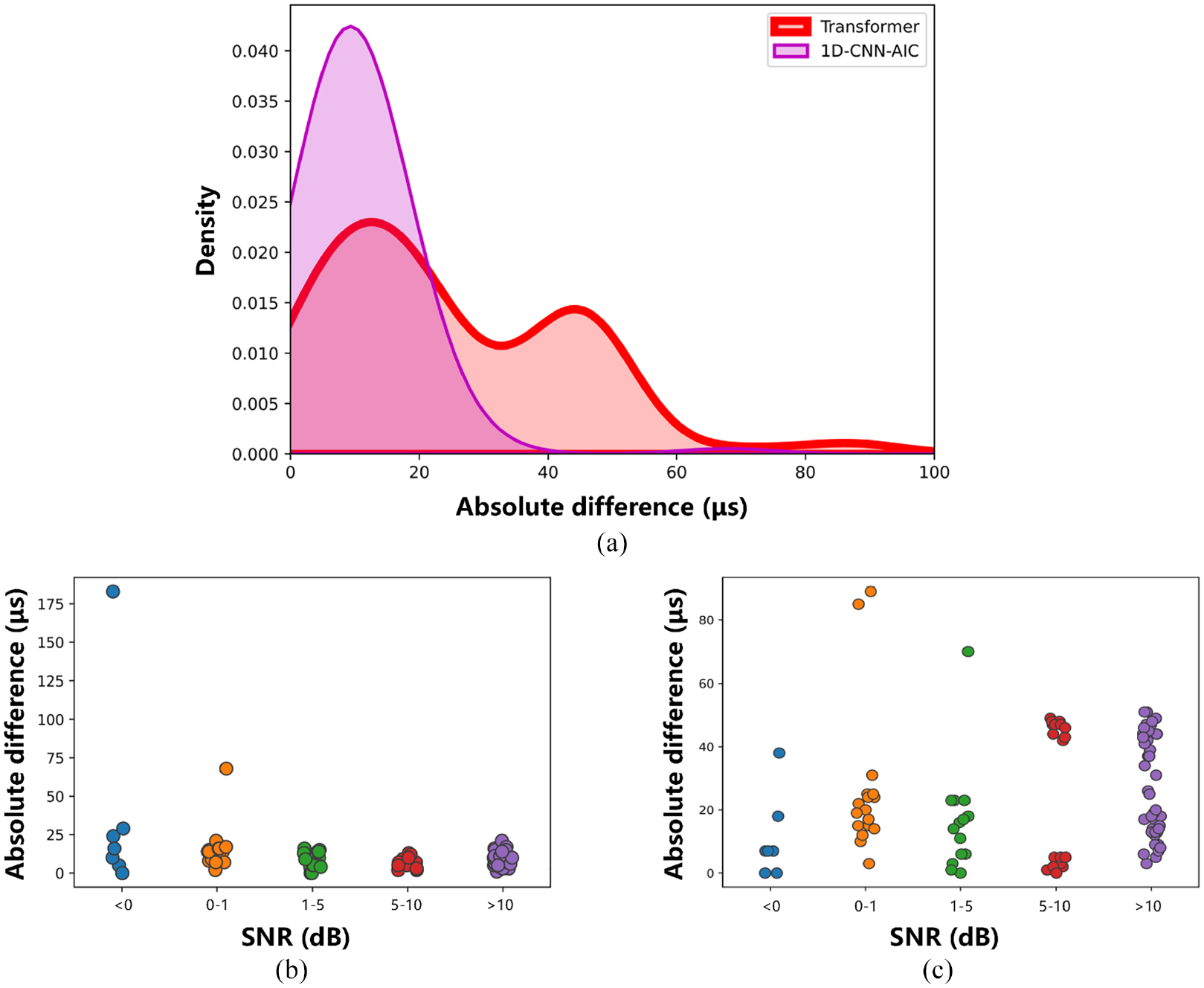
Density diagram and scatter plot of the proposed method and 1D-CNN-AIC method in group C: (a) density diagram of the two method, light purple curve and region represent 1D-CNN-AIC and darker ones represent the proposed method, (b) the scatter plot of the 1D-CNN-AIC method at each SNR interval, (c) the scatter plot of the proposed method at each SNR interval.
The precisions presented by the Transformer-based recognition method are close to the 1D-CNN-AIC method; however, the former one has non-negligible advantages in data preprocessing and feature calculation: (1) The Transformer structure applied by the proposed method can make up for the shortcomings of 1D-CNN in feature extraction via a more powerful computational strategy. The latter one requires utilizing multiple characteristics to enhance the spatio-temporal correlation of the data. This complex calculation process takes up a lot of computer storage, while the Transformer directly applies the original data, which greatly simplifies the data preprocessing steps; (2) Moreover, under the same hardware condition and software configuration, the determination process of 1D-CNN-AIC takes 41 s in total, while that of proposed method only needs 11 s, which greatly improves the determination efficiency and is closer to the actual application. The Transformer-based method has higher recognition efficiency with the approximative performance.
Numerical comparison with 1D-CNN-AIC, AIC, STA/LTA-AIC and FT
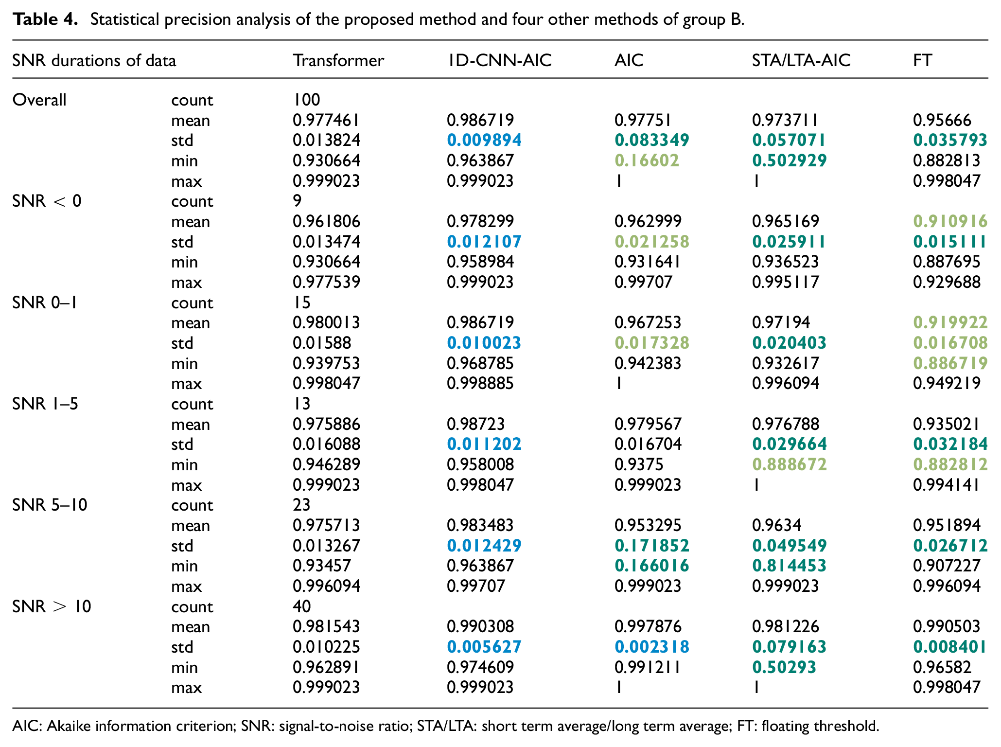
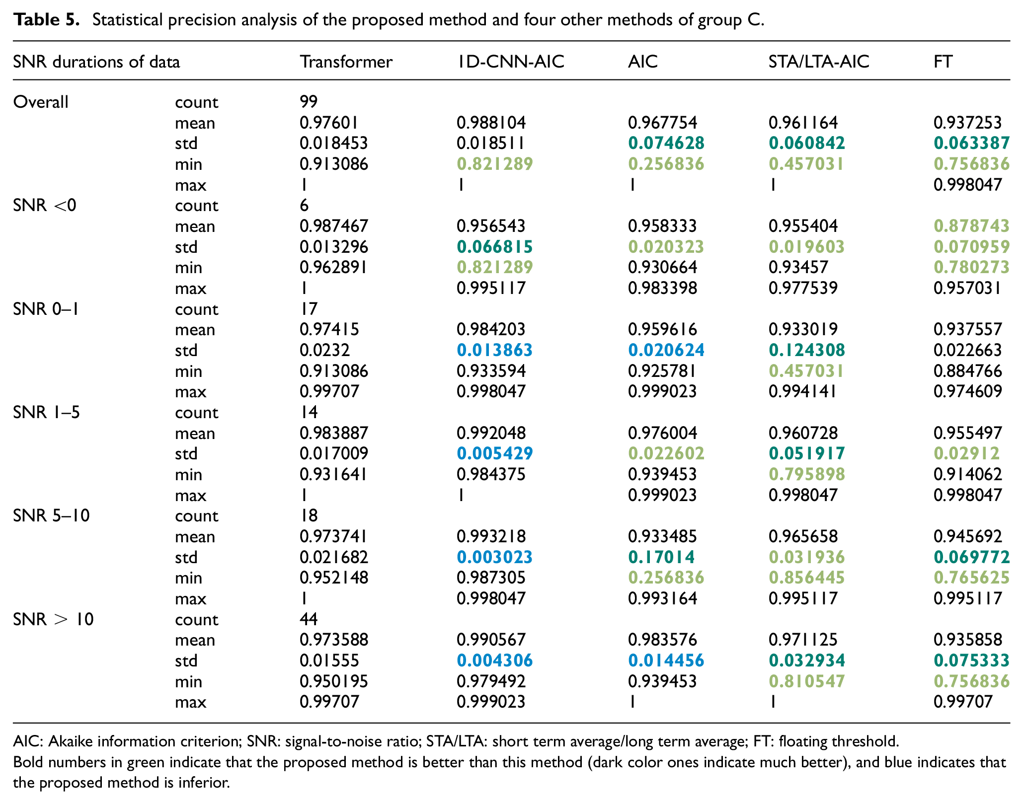
Tables 4 and 5 shows the statistical precision performance of the proposed method and four other methods. The count of the corresponding parameter (noted as count), mean precision value of the corresponding interval (noted as mean), standard deviation of the corresponding interval (noted as std), minimum precision value of the corresponding interval (noted as min), and maximum precision value of the corresponding interval (noted as max) are listed in both tables. The precision is expressed as Equation (17):
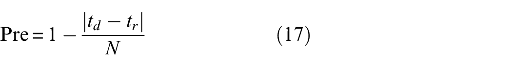
where
Statistical precision analysis of the proposed method and four other methods of group B.
AIC: Akaike information criterion; SNR: signal-to-noise ratio; STA/LTA: short term average/long term average; FT: floating threshold.
Statistical precision analysis of the proposed method and four other methods of group C.
AIC: Akaike information criterion; SNR: signal-to-noise ratio; STA/LTA: short term average/long term average; FT: floating threshold.
Bold numbers in green indicate that the proposed method is better than this method (dark color ones indicate much better), and blue indicates that the proposed method is inferior.
The values of the other four methods are used to compare with the values of the proposed method (std calculates the growth rate, and other statistics calculate the growth value), and the corresponding blank will be marked when the number exceeds 5% (or 0.05 for statistics other than std). Bold numbers in green indicate that the proposed method is better than this method (dark color ones indicate much better), and blue indicates that the proposed method is inferior.
It can be seen from the table that the proposed method has better performance and more stable results than AIC, STA/LTA-AIC and FT. For the 1D-CNN-AIC method, the proposed method is only slightly insufficient in std value (i.e., stability), but other values are not significantly different. The overall difference is below 2%, which is in the acceptable range. In summary, the proposed Transformer-based method has relatively robust performance.
In order to better demonstrate the proposed method and prove its potential application in AE source localization, the identified source locations are calculated based on the arrival times and spatial sensors positions obtained by each method, and presented as mean error scores which are listed in Table 6. As shown, compared to other methods, the proposed method maintains a localization accuracy error of around 10% (group C is even better at around 8%), with good stability. The identification error rate is acceptable, but the advantages are not prominent enough under high SNR data. Further improvements on both identification and localization methods in future work would lead to additional enhancements.
Statistical localization precision analysis with error score of the proposed method and four other methods of group B and C.
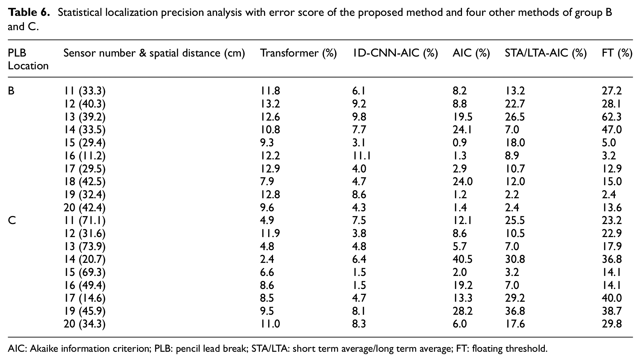
AIC: Akaike information criterion; PLB: pencil lead break; STA/LTA: short term average/long term average; FT: floating threshold.
Conclusion
In this paper, a Transformer-based method for determining the onset time of AE is proposed. It contains a Transformer model, which is used to extract the features of the sample points of the waveforms. The index of the point in the Transformer-processed sequence that first reaches the maximum value is obtained as the arrival time, and the whole identification process is simple. In particular, in the data preprocessing stage, the integrating labeling strategy with thresholds is used, which greatly reduces the training complexity, makes the data in small segments form better reflect the arrival status of the current point, and optimizes the model performance. The performance of this method is evaluated by analyzing the distribution of results via testing. This method can learn the characteristics of the acoustic waveform in the time dimension well, and the arrival time pickup performance is kept within 40 μs. For signals with low SNR, the method in this paper has strong adaptability, and the picking result is very close to manual picking. This method is not only superior to several common determination methods, but also greatly improves the efficiency.
The method in this paper is designed based on laboratory AE data, and the performance of low SNR signals is interesting in the case of small data set. Moreover, the algorithm does not conflict with multi-sensor systems. Each of the multiple co-existing signal sources would be processed as an individual input and undergo the similar algorithmic process. The approach is independent of any different time domain characteristics they may exhibit while it’s the original signals themselves the authors are concerned about.
However, there are still drawbacks to overcome. Due to the small-scale data used for model training, waveforms with low SNR type may not be fully learned. The determination step can be further improved to enhance the precision. Increasing the network depth and improving the model parameters may also improve the performance of this Transformer-based method.
Footnotes
Acknowledgements
The PLB AE data provided by Prof. Madarshahian played a very important role in the development of this article. The author would like to thank him for making the data public.
Declaration of conflicting interests
The author(s) declared no potential conflicts of interest with respect to the research, authorship, and/or publication of this article.
Funding
The author(s) disclosed receipt of the following financial support for the research, authorship, and/or publication of this article: This project is supported by the National Natural Science Foundation of China (Grant No. 51905335) and the Shanghai Science and Technology Committee Research Project (Grant No. 19040501500). The Transformer training part mentioned in this paper relies on Google Colaboratory, a cloud computing platform developed by Google, which enables the Transformer model training to run on computers with any hardware configuration, and makes it possible for the proposed method to be applied on the mobile terminals. The scientific and high-quality PLB data provided by Prof. Madarshahian played a very important role in the validation and analysis part of this paper.