Structural health monitoring of a lenticular truss bridge: a comprehensive study

Abstract

The combined use of finite element modeling and structural health monitoring is becoming increasingly relevant in bridge maintenance. A growing number of new and old structures is instrumented with different kinds of sensors driven by dedicated hardware and software, while numerical models are used to simulate the response of the structures under various scenarios. This paper presents the monitoring of the Smithfield Street Bridge, one of the oldest and most iconic bridges in the city of Pittsburgh (Pennsylvania, USA). The bridge was instrumented by an independent party, not involved with the research presented here, with strain, displacement, and rotation wireless sensors. A detailed finite element model of one of the spans of the bridge was developed to calculate the strains induced by standardized trucks under pristine and simulated damage conditions. In addition, the model enabled to determine the sensitivity necessary to detect relevant structural changes in the bridge. The results of the numerical analyses were then compared with the results of a test in which a truck of known weight crossed the bridge multiple times. Finally, the data relative to 3 years of uninterrupted monitoring were processed and analyzed to identify eventual anomalies.

Keywords

Structural health monitoring bridges finite element modeling wireless sensing systems

Introduction

According to the Federal Highway Administration (FHWA),¹ there are over 600,000 highway bridges (A highway bridge is a public vehicular structure more than 6.1 m (20 feet) in length that spans an obstruction or depression). in the United States (U.S.). Each bridge is assigned with a single-digit number (0–9) that describes the physical condition of its main parts, and the bridge’s overall status is determined by the lowest rating among deck, superstructure, substructure, or culvert.² If the lowest rating is greater than or equal to 7, the bridge is classified as good; if it is less than or equal to 4, the asset is denoted as poor. Bridges rated 5 or 6 are classified as fair.^3,4 Currently, 42% of the U.S. bridges are at least 50 years old, and 7.5% of them are labeled in “poor” condition.⁵ The 2021 report card from the American Society of Civil Engineers (ASCE)⁵ stated that while structurally poor (ASCE uses the term structurally deficient) bridges “are not inherently unsafe, they require substantial investment in the form of replacement or significant rehabilitation, and they present higher risk for future closure or weight restrictions.”

In the U.S., each bridge must be visually inspected at least once every 2 years,⁶ and sometimes nondestructive evaluation (NDE) methods, such as liquid penetrant, magnetic particles, etc., complement the visual inspection. However, periodic inspections may miss the onset of critical issues between two consecutive inspections. This is raising the attention towards cost-effective structural health monitoring (SHM) strategies that evolves the maintenance paradigm from time-based NDE in which a structure is inspected periodically, to permanent-based where sensors monitor 24/7 the asset to flag, locate, and quantify damage as it happens. The sensors measure physical characteristics such as strain and acceleration, just to mention a few, while dedicated hardware/software process the time series streamed from the sensors. Strain is the most frequently monitored parameter in bridge health monitoring.⁷ Strain-based approaches were among the first to be explored and applied because strain is directly related to stress and deflection, which reflect structural performance, safety, and serviceability. Strain field anomalies are frequently indicators of unusual structural behaviors.⁷ One of the advantages of strain-based SHM is that the sensors to measure deformation exist in many different kinds and can be electrical-based or optical-based. In addition, these sensors can be applied on or within any type of structure and any construction material using bolts, adhesive epoxy, or even in a non-contact-based fashion. The many notable examples of strain-based SHM were reviewed in an excellent paper by Glisic.⁷

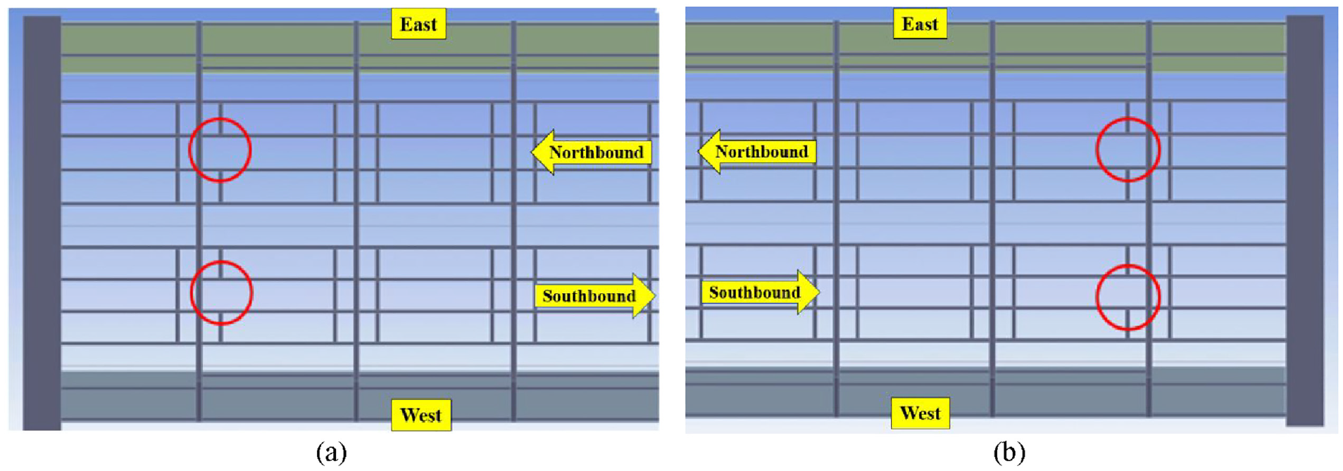
In 2017, the Pennsylvania Department of Transportation (PennDOT) started a pilot bridge instrumentation program. Ten bridges across south and southwest Pennsylvania were instrumented during the period 2017–2019 with an array of commercial wireless sensors capable of providing real-time information about static and (for some bridges) dynamic responses. The installations were completed by a company, hereinafter referred to as the Vendor, not involved in the study presented here. The Vendor owns and maintains the sensors and the associated hardware and software. One of the bridges included in this pilot program is the iconic Smithfield Street Bridge, built nearly 140 years ago in the city of Pittsburgh. The bridge consists of seven spans, two of which are supported by riveted built-up lenticular through-trusses structures (Figure 1). The bridge connects Pittsburgh downtown to the Southside neighborhood across the Monongahela River. The bridge was instrumented with wireless strain gages, displacement sensors, tiltmeters, and a few accelerometers. A few days after installation, the Vendor performed a controlled truck load test.

Figure 1.

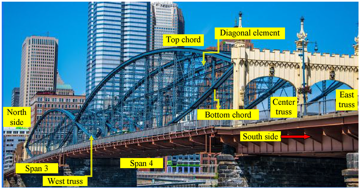
The Smithfield bridge with directions and nomenclature. Span 4 was the subject of this study.

In this paper, a holistic study of the bridge was conducted by combining finite element (FE) modeling and analysis of the SHM data. A high-fidelity FE model of the lenticular through-trusses was developed using the commercial software ANSYS^®. The scope was to determine the required sensitivity to detect subtle changes in the structure, and to simulate a few loading scenarios under pristine and simulated damage conditions. Specifically, the model was used first to predict the static deformation along two control members of the truss caused by the individual crossing of three American Association of State Highway and Transportation (AASHTO) standard trucks. The load of a truck identical to the one used by the Vendor for the load test was simulated, and the results were compared to the experimental measurements made available to the authors by the research sponsor. Then, the strains induced by an AASHTO truck under pristine and simulated damage were computed at the location of the gages. Finally, three data-driven analyses were conducted using the data stored in a password-protected repository, in order to identify existing structural anomalies or precursors of future issues. In the first analysis, the strains and the temperatures were examined to quantify the structural deformation of the structure to thermal loading. Then, the effect of the temperature on the recorded strains was mitigated using a simple procedure to extract and isolate the effects of live loads. The term “live load” is used hereafter to indicate traffic load or any transient rapid event, such as impact, occurring on the bridge during normal operation. Finally, the live loads data were coupled to an unsupervised learning class based on outlier analysis (OA) to identify notable transient events. The use of unsupervised learning in data-driven SHM offers the fundamental advantage that the information on the damage conditions do not need to be known already, contrarily to the supervised learning class. Unsupervised learning algorithms only require a sufficiently large number of data that includes all possible baseline configurations, whereas supervised methods require data from damaged configurations, which cannot always be realistic in practice.^8–10 OA was chosen to leverage the experience of one of the authors, who demonstrated the effectiveness of the analysis at detecting damage in bridges,¹¹ plates,^12,13 cables,¹⁴ and rails.¹⁵

The use of commercial FE software to model a bridge in support of SHM applications is not novel. A review by Rizzo and Enshaeian¹⁶ about bridge health monitoring programs in the U.S. has shown that perhaps the most comprehensive analyses, including load truck tests, involved the I-35W St. Anthony Falls Bridge in Minnesota and the Charles W. Cullen Bridge (Indian River Inlet Bridge) in Delaware. Both bridges are relatively new. The I-35W St. Anthony Falls Bridge opened in 2008 and was instrumented with more than 500 sensors to gage deformations, temperature, vibrations, expansion, and corrosion.¹⁷ Linear elastic FE models were created in ABAQUS and validated using truck-load tests.¹⁸ French et al.¹⁷ investigated the time-dependent (creep and shrinkage) and temperature-dependent behavior of the bridge to prevent excessive loss of post-tensioning that may yield to concrete cracking or large deflections. They used a combination of laboratory creep and shrinkage tests, FE analyses, and in situ monitoring of longitudinal deflections and strains using the first 5 years of bridge operation. The results of this investigation were used to develop a prototype monitoring system for the bearing movements using data from linear potentiometers located near the expansion joints of the bridge. Interested readers are referred to Refs. 17–22 for a holistic view of the program.

The Charles W. Cullen Bridge opened in 2012 and included a comprehensive SHM system based on strain sensors, accelerometers, tiltmeters, displacement sensors, anemometers, and chloride sensors.^23–26 Al-Khateeb et al.²⁶ presented the results of six load tests performed just prior to the bridge’s opening, and then again at 6 months, 1, 2, 4, and 6 years. The results of the first two tests constituted the baseline, for the second test proved that the bridge response stabilized. In order to eliminate any initial offset, the time-history record was first “zeroed” by taking the average of the first 25 data points and subtracting that value from the entire time history. Then, a moving average was computed using a window of 25 data points to eliminate the inherent low-level noise in the sensor data. Finally, the maximum and minimum (i.e., peak) values of the record were determined. At the end of the sixth year, Al-Khateeb et al.²⁶ reported that the comparisons of a few relevant features such as time histories and peak values indicate that the bridge condition had remained unchanged. Although the data contained some variabilities, no trends were observed. Natalicchio²⁷ built and calibrated a 3D FEM in STAAD.Pro using empirical strain data from the controlled load tests. The calibrated parameter was the elastic modulus of the edge girders. Through various iterations, the model of the bridge showed good results when compared to the SHM strain response and the concrete edge girder 56-day compressive strength tests. The model was validated using different loading configurations, and it proved to be a closer representation of the structure.

A few other worldwide examples^28–35 are presented here for the sake of completeness. Yu and Ou²⁸ used the data from 112 sensors to update a model of the Aizhai suspension bridge. Schlune et al.²⁹ modeled the new single-arch Svinesund Bridge and its health was evaluated using static and dynamic measurements. He et al.³⁰ used ANSYS^® to create a 3-D model of the Nanjing Yangtze River Bridge. The model was updated using stress-time histories. Another 3-D model was built by Duan et al.³¹ for the Tsing-Ma cable suspension bridge in order to estimate and compare the amount of strain and stress experienced by important bridge members. Gatti³² combined FE modeling and static and dynamic field data to study a prestressed reinforced concrete. Schommer et al.³³ considered the SHM of a prestressed concrete beam leveraging a FE model and static and dynamic responses. Recently, Venuti et al.³⁴ created two different FE models of the pedestrian Streicker Footbridge at the campus of Princeton University. A three-dimensional beam-based model was developed to represent the complex behavior of the full-scale benchmark bridge. The model of the bridge deck was then refined using shell elements. The Commodore Barry Bridge is the longest cantilever bridge in the U.S.³⁵ It has a total length of 4240 m and a main span of 501 m. Vibrating-wire accelerometers, strain sensors, weigh-in motion devices, and tiltmeters were installed.³⁶ Pines and Atkan³⁷ used this bridge as a testbed for the framework of a supervisory control and data acquisition system (DAQ) system for SHM applications. Catbas et al.³⁵ developed a reliability model considering dead load, wind pressure, traffic loads, temperature effects and their combinations. The scope was to assess how bridge health monitoring can be used to minimize the uncertainties related to phenomena which are difficult to model. They found that temperature effects, that is, expansion and contraction due to temperature increase and decrease, cannot easily be conceptualized and therefore modeled. They observed that the peak-to-peak strain differential due to thermal-induced strain was around 400 µε, that is, 10-fold higher than the maximum strains induced by traffic.

The scientific contribution of this paper lays on the holistic approach taken to monitor an old iconic bridge. An extensive numerical analysis of the pristine bridge and of the bridge with a few simulated damage scenarios was completed using a high-fidelity model. The reliability of the model was proven by comparing some numerical results with the experimental measurements taken with an array of wireless sensors during a controlled truckload test. In addition, the measurements relative to 3 years of monitoring were examined using an ad hoc signal processing to successfully identify non-critical structural anomalies. To the best of the authors’ knowledge,¹⁶ there are very few reported cases in which a given bridge in the U.S. was monitored for as long as 3 years. Moreover, those specific long-term monitoring programs were not complemented with FE data that support field evidence and did not quantify the effects of truck load. Finally, it is emphasized that the present article is completely different than the work presented in Ghahremani et al.¹¹ While paper¹¹ is about a pre-stressed concrete box bridge, the present article is about a lenticular truss bridge structure. While both papers share the same idea of creating a high-fidelity FE model, the study presented in this article provides insightful information about the effects of different truck loads at different positions, about the strains streamed from a network of wireless strain gages, and about the effect of simulated damage. Finally, the study presented in Ghahremani et al. did not consider any effect of damage.

The paper is structured as follows. Next section provides a brief historical account of the Smithfield Street Bridge along with a few structural details, and a description of the monitoring system installed in the year 2019. Section “The FE model” describes the FE model and the static analyses that were computed. Section “Structural health monitoring algorithms” presents the results of the long-term monitoring of the bridge. The focus is on the analysis of the data extracted from the strain gages bonded to the superstructure. Finally, section “Conclusion” ends the article with some concluding remarks and recommendations for future research.

The structure and the health monitoring system

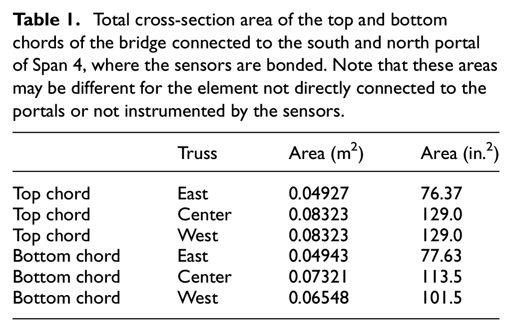
The Smithfield Street Bridge was built between 1881 and 1883, widened in 1889, and widened again in 1911. The whole structure is 542 m (1777 feet) long and consists of seven spans and two lanes each bound. The iconic parts of the Bridge are Span 3, close to downtown, and Span 4, close to the south side neighborhood. The superstructure of Span 4 is the subject of this study, including the FE modeling. The superstructure of Spans 3 and 4 are made of riveted built-up lenticular through-trusses. For convenience, each lenticular truss is labeled as the west, center, and east trusses (Figure 1), and several close-up photos are presented in Figure 2. Span 4 is pinned north and has an expansion joint on its south end. Each truss is composed of three main parts: the top chord, the bottom chord, and the diagonal element. The top chord is formed by four I-shaped steel members riveted together. The bottom chord is formed by a variable number (six to eight) of bars pinned together. The diagonal element is instead a single bar. Table 1 lists the areas of the cross-section of those elements instrumented with the wireless strain gages.

Figure 2.

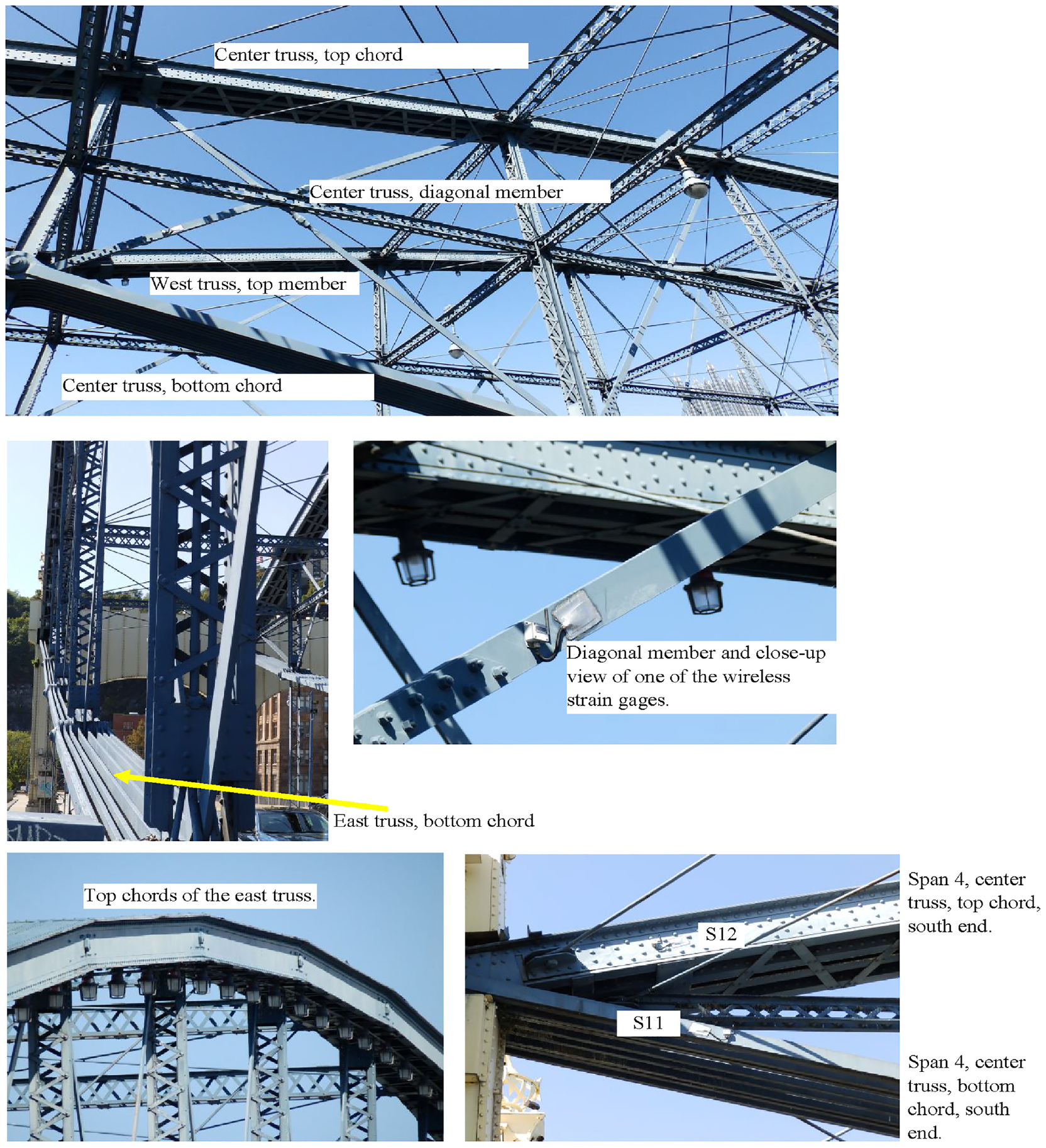
Close-up view of the center truss, with the top, diagonal, and bottom members. The west truss and some strain gages are also visible. Photos by Piervincenzo Rizzo.

Table 1.

Total cross-section area of the top and bottom chords of the bridge connected to the south and north portal of Span 4, where the sensors are bonded. Note that these areas may be different for the element not directly connected to the portals or not instrumented by the sensors.

	Truss	Area (m²)	Area (in.²)
Top chord	East	0.04927	76.37
Top chord	Center	0.08323	129.0
Top chord	West	0.08323	129.0
Bottom chord	East	0.04943	77.63
Bottom chord	Center	0.07321	113.5
Bottom chord	West	0.06548	101.5

In July 2019, the Vendor, which was not involved in the study presented here, instrumented Span 4 with 30 strain gages, seven displacement sensors, three high-resolution tilt sensors, four accelerometers, a data logger, and a remote communication gateway. Each sensor embedded a temperature detector. Figure 3 shows the location of the 18 strain gages bonded to the trusses. Although the top chord is likely not acting as a pure truss member subjected to pure axial load, it may be argued that sensors S01, S06, S07, S12, S13, and S18 are bonded at the neutral axis and therefore subjected to the stress associated with the axial force. The remaining 12 gages were bonded to the south portal, four on each of the three columns of the portal, one on each face of each column. It is noted here that the 12 strain gages on the portal and the other kinds of sensors are not part of the study presented in this article and are ignored hereinafter. The wireless strain gages use proprietary sensing, are self-adhesive type, do not require drilling, and have an accuracy of 1 µε. Each sensor has an adjustable trigger from 16 to 512 µε and the sampling rate can be changed from 10 to 200 ms. The gages are temperature compensated and contain the following additional sensing: temperature, battery voltage, and wireless signal strength. According to the manufacturer, typical measurements occur every 20–25 ms. If strain variation exceeds a preset threshold (minimum of about 30–40 µε) in a short period of time (∼100 ms) and the strain level remains high or low for about 200 ms a strain event packet is generated and sent with the same rate (20–25 ms). If gage does not detect any event, strain readings will be captured on fixed intervals (e.g., 8 s), and transmitted on the next transmission interval (e.g., 6 min).

Figure 3.

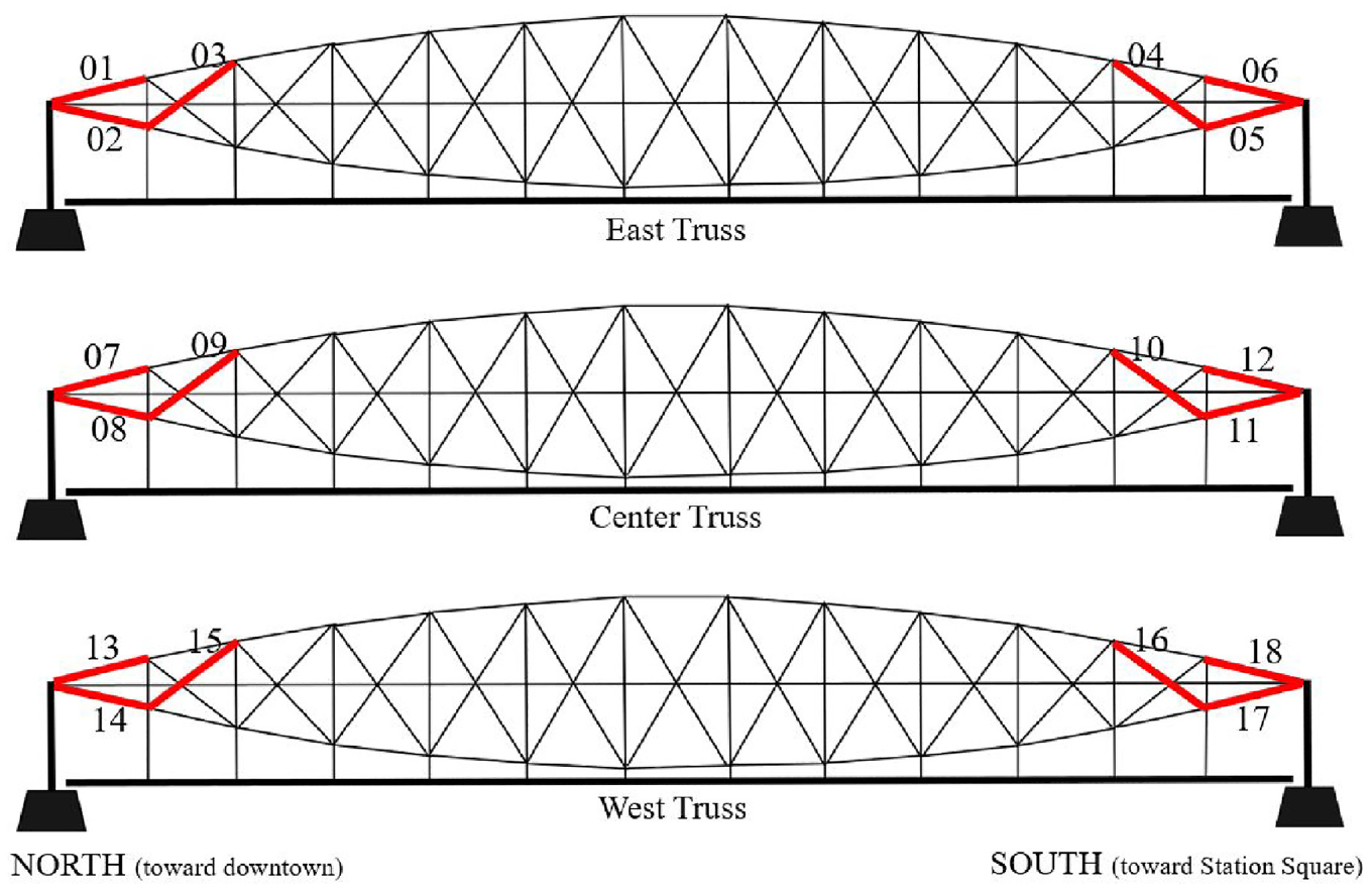
Drawings of the east, center and west trusses. The members instrumented with a wireless strain gage are labeled according to the gage number. The sensors on the east truss face west, whereas the gages on the center and west truss face east.

Shortly after installation, a truckload test was performed using a 26,272 kg (57,920 lb) truck. The steer axle was 7992 kg (17,620 lb) and the drive “tandem” axles were 18,280 kg (40,300 lb). First, the truck traveled northbound twice (Tests 1 and 2) crawling at about 8 km/h on the left lane. Then, the truck stopped at both ends of Span 4. Tests 1 and 2 were repeated with the truck crawling northbound on the right lane (Tests 3 and 4). After that, the truck was directed southbound, and Tests 1 to 4 were replicated and are labeled as Tests 5 and 6 (right lane) and Tests 7 and 8 (left lane). The largest difference between the strain with and without the truck at each gage during each test run was calculated and reported by the Vendor, and summarized in Figure 4. The figure shows that the monitored top chords are in compression, whereas the other elements are in tension. With the exception of the south diagonal member and the bottom chord of the east truss, the deformations at the west truss were smaller than those at the east.

Figure 4.

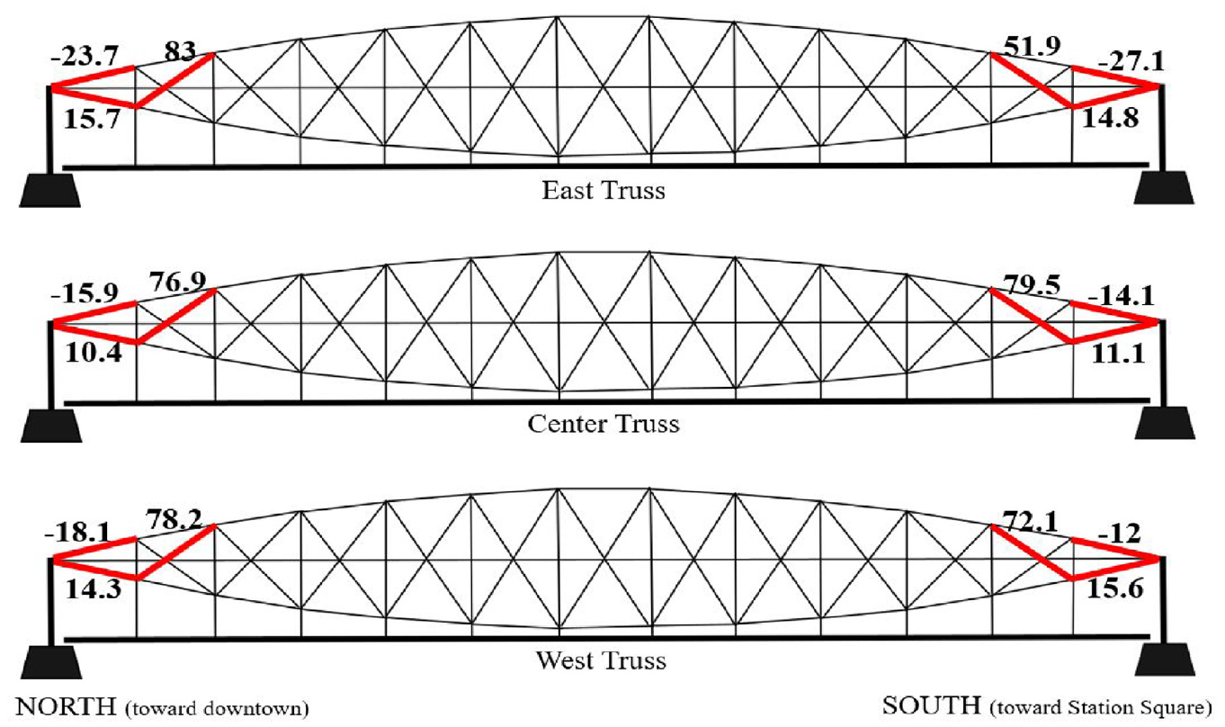
Maximum strain increase measured by each strain gage during the truck load test. The values are expressed in microstrains. The values were reported by the Vendor performing the test in a document made available to the authors by the sponsor of the research.

The FE model

Numerical setup

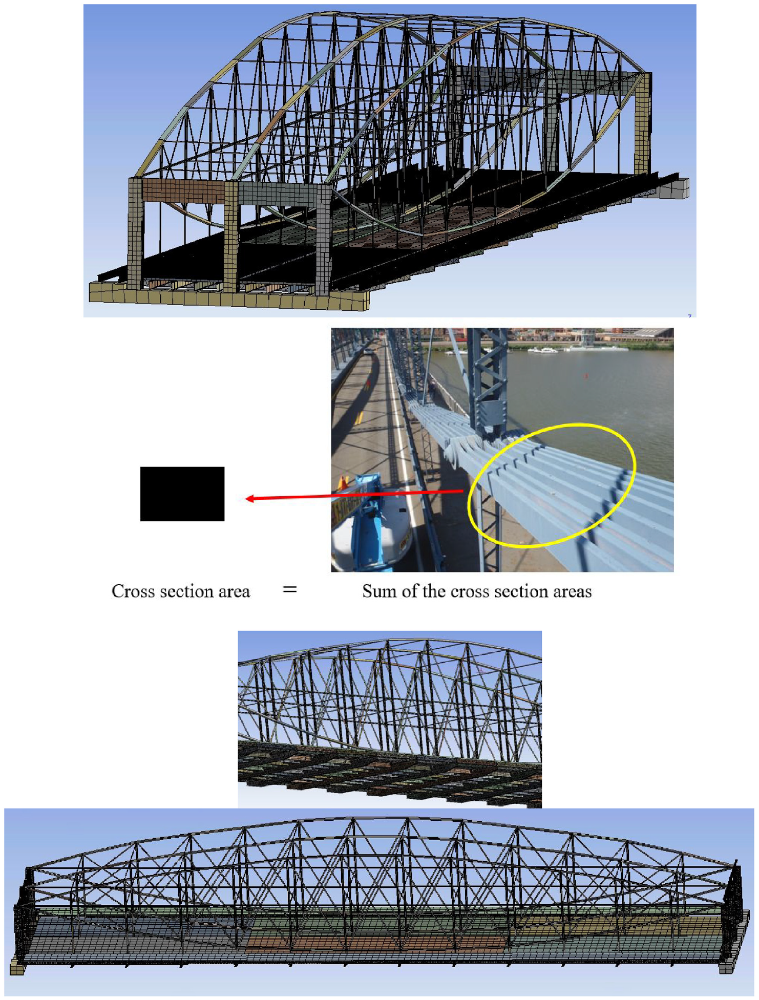
The high-fidelity FE model of the superstructure and the deck of Span 4 was created in ANSYS 2020 R2 using drawings provided to the authors by PennDOT. The model contained more than 17,000 components, most of which are connector members. To make the static analysis computationally manageable, the following few simplifications were made: (1) the small longitudinal components found under the deck and the stiffeners of the floorbeams were not modeled; (2) the splice plates and a few other connection members were neglected; (3) the rebar of the concrete deck were replaced by a steel plate under the deck; (4) the portals were approximated; (5) the bottom chord was modeled as a single 203.2 × 254 mm² (8″ × 10″) steel bar instead of the actual ten 203.2 × 25.4 mm² (8″ × 1″) bars; (6) the top chord became a rectangular element with the cross-section area equal to the total cross-sectional area of the true chord. The model used in the analyses consisted of 880 structural components, more than 244,700 FEs, and over 698,700 nodes. The number of nodes is the result of a tradeoff between convergence of the results and computational time/cost. Some screenshots of the FE model are presented in Figure 5. For the material, the Young’s modulus of structural steel (200 GPa, 29,000 ksi), and the typical type A concrete (24.1 GPa, 3500 ksi) were considered.

Figure 5.

Screenshots of the finite element model of the Smithfield Street Bridge.

Trucks simulations

Three AASHTO trucks, namely the ML-80, the H20, and the HS20 were selected. A fourth truck, identical to the truck used to perform the load test, was considered. The weight and the relative axles distance of the four trucks are schematized in Figure 6. The static analyses calculated the deformation generated by each individual truck on the two diagonal members hereinafter labeled as L₁U₂ and L₁′U₂′, monitored with strain gages S09 and S10, respectively. These members are considered control members because they sustain the largest stress among the components being monitored. Each truck was placed on the northbound left lane. A few truck positions were considered to identify the location that maximizes the deformation of the control members. Figure 7 provides a close-up view of the setup relative to the AASHTO ML-80 truck, near to member L₁U₂, that is, close to the north end of Span 4. The distance of the rear wheels from the north portal ranged between 7.620 and 15.24 m at 1.27 m interval (Table 2). The table shows that the largest numerical load and strain resulted to be equal to 76.15 kN (17.12 kips) and 114.1 µε, respectively, when the rear axle of the truck was 10.16 m (400 in.) away from the north end. Based on the information available to the authors, the steel used for the control members has a nominal yield stress σ_Y equal to 228 MPa (33 ksi) and Young’s modulus equal to 200 GPa (29,000 ksi), which implies that the yield strain is equal to 1138 µε. The above static analysis may be combined with conventional approaches to determine any future load rating and load posting of the bridge.

Figure 6.

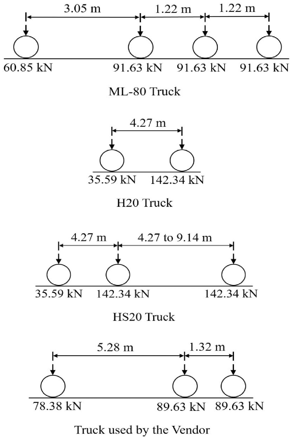
Schematics of the trucks simulated in this study. The top three are AASHTO trucks, whereas the bottom truck has the same characteristics of the vehicle used by the Vendor to test the bridge.

Figure 7.

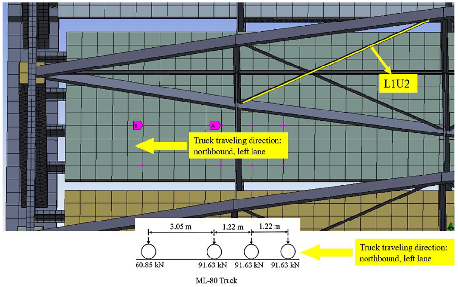
Numerical setup relative to the analysis of the ML-80 AASHTO truck. The pink dots locate the position of the truck wheels.

Table 2.

Numerical simulations. Position of the rear axle of the ML-80 AASHTO truck from the north end of Span 4, and corresponding induced force and strain on the control member L₁U₂. The distances are expressed in m. (in.) and the forces are expressed in kN (kip).

	Distance of rear axle from north portal	Axial force at member L₁U₂	Axial strain at member L₁U₂ (με)
Position 1	15.24 (600)	39.26 (8.83)	58.84
Position 2	13.97 (550)	53.93 (12.12)	80.83
Position 3	12.70 (500)	65.89 (14.81)	98.75
Position 4	11.43 (450)	73.69 (16.57)	110.40
Position 5	10.16 (400)	76.15 (17.12)	114.10
Position 6	8.89 (350)	72.67 (16.34)	108.90
Position 7	7.62 (300)	63.77 (14.34)	95.57

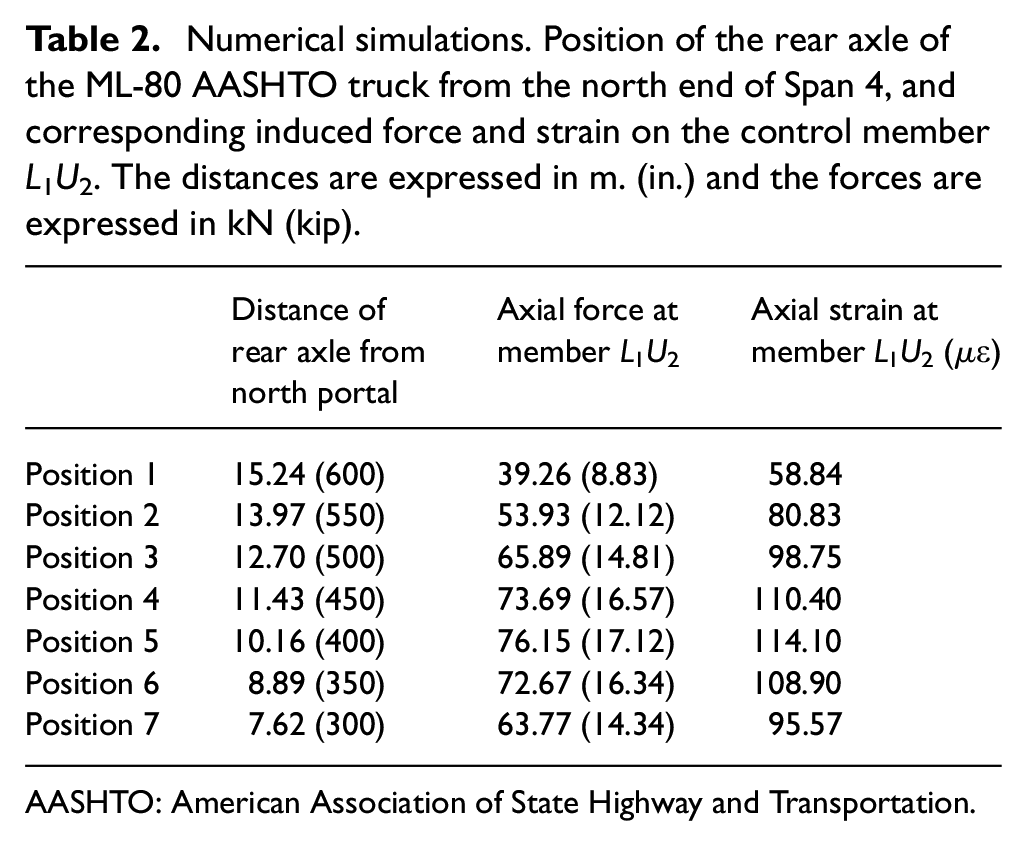
AASHTO: American Association of State Highway and Transportation.

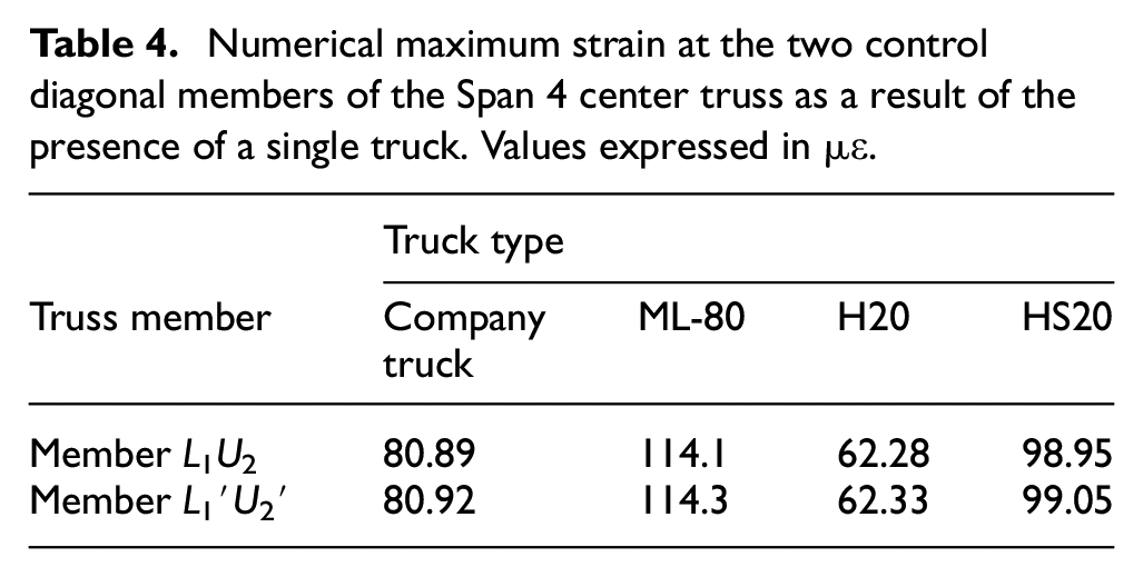
The same approach was applied to calculate the largest values on the diagonal member close to the south side of the bridge. Table 3 summarizes the positions of the truck and the corresponding load and strain. As expected, the calculated values are nearly identical to those relative to the north side of Span 4. The small difference (<1%) is likely due to the spatial resolution (1.27 m) of the longitudinal position of the truck. The same numerical analysis was applied using the other three trucks. The maximum calculated strains in the two diagonal members of the center truss are presented in Table 4. Owing to the linearity of the model, the numerical deformations are proportional to the weight of the truck. It must be noted though that the points of application of the forces, that is, the position of the wheels, differ from truck to truck along the longitudinal direction but the distance of the right wheels from the parapet are the same.

Table 3.

Numerical simulations. Position of the rear axle of the ML-80 AASHTO truck from the south end of Span 4, and corresponding induced force and strain on the control member L₁′U₂′. The distances are expressed in m. (in.) and the forces are expressed in kN (kip).

	Distance of rear axle from south portal	Axial force at member L₁′U₂′	Axial strain at member L₁′U₂′ (με)
Position 1	1.27 (50)	37.88 (8.85)	56.77
Position 2	2.54 (100)	52.20 (11.74)	78.23
Position 3	3.81 (150)	64.36 (14.47)	96.46
Position 4	5.08 (200)	72.84 (16.38)	109.17
Position 5	6.35 (250)	76.27 (17.15)	114.31
Position 6	7.62 (300)	73.80 (16.59)	110.61
Position 7	8.89 (350)	65.58 (14.74)	98.28

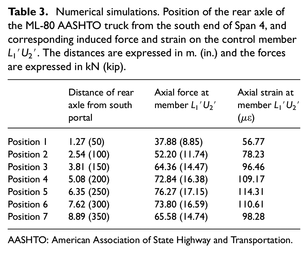
AASHTO: American Association of State Highway and Transportation.

Table 4.

Numerical maximum strain at the two control diagonal members of the Span 4 center truss as a result of the presence of a single truck. Values expressed in µε.

	Truck type
Truss member	Company truck	ML-80	H20	HS20
Member L₁U₂	80.89	114.1	62.28	98.95
Member L₁′U₂′	80.92	114.3	62.33	99.05

Numerical versus experimental results

The FE results relative to the truck used in the field were compared to the experimental results reported by the Vendor. The case of crossing the northbound left lane twice is presented here. The strains measured by sensor S09, bonded to the diagonal member L₁U₂ (see Figure 3) were equal to 67.0 and 66.9 µε. These values are about 17% lower than the calculated numerical deformation of 80.9 µε listed in Table 4. The experimental values recorded by S10, bonded to the diagonal member L₁′U₂′, were equal to 71.5 and 71.2 µε, which are, only 12.3% lower than the numerical prediction of 80.9 µε. The difference between the numerical and the experimental value is likely due to a discrepancy between the numerical and the real (but unknown) lateral distance of the truck from the east parapet. To prove this hypothesis, we placed the same truck 1.91 m (75 in.) away from the centerline instead of 0.89 m (35 in.) to be discussed in section “Trucks simulations.” The numerical strain of member L₁U₂ is now 69.2 µε, just 3.3% higher than the experimental values recorded by S09. Similarly, when the numerical truck is 1.27 m (50 in.) from the center truss, the calculated strain of member L₁′U₂′ is equal to 77.09 µε, just 7.8% higher than the recorded values from gage S10. The outcome of this analysis is that a direct comparison between the FE estimation and the experimental measurements suffers from the lack of knowledge about the exact lateral position of the truck. Nonetheless, the agreement between the numerical and the experimental results is quite good and proves the reliability of the model.

Further numerical analyses

According to the drawings available to the authors, each truss is symmetric with respect to the midspan, but the distance between the west and the center truss is about 305 mm (12 in.) shorter than the distance between the east and the center truss. In addition, as seen in Table 1, the total cross-sectional area of the chords is not the same for all trusses. To quantify the effects of these differences on the deformation of the instrumented members, four concentrated forces were equidistant from the midspan and the centerline, as if two wheels were on the northbound lane and two wheels were on the southbound lane. Each force was 44.5 kN (10 kips), and the relative longitudinal and lateral distance were equal to 2.54 m (100 in.). The resulting strains are visualized in Figure 8, and prove the symmetry of the bridge with respect to its midspan. However, the strains at the east truss are higher than at the corresponding elements of the west truss. For example, the deformation at the north east top chord is −4.26 µε, nearly double the deformation of the north west top chord (−2.42 µε). These numerical findings are consistent with the fact that the total cross-sectional area of the top and bottom east chord is smaller than at the west chords.

Figure 8.

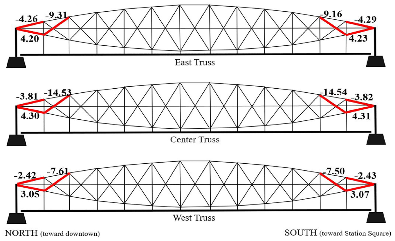
Numerical strains induced by a four-points load centered at midspan at equidistance from the centerline. The values are expressed in microstrains.

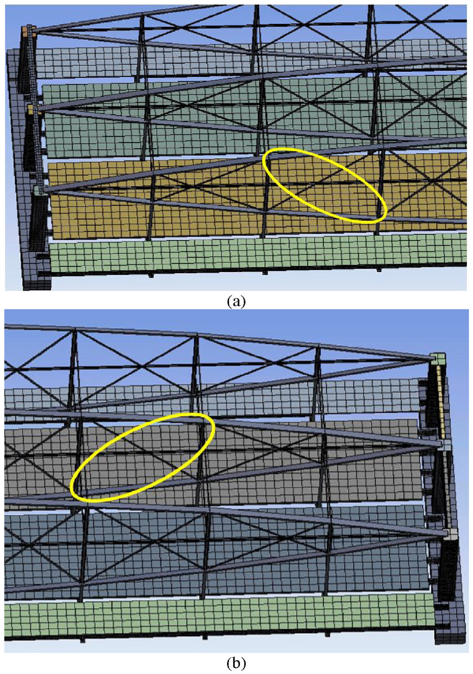
Finally, two damage scenarios were simulated and their effects under certain truck crossings were calculated and compared to the corresponding pristine deformations. The first damage scenario was the removal of four transverse diaphragms: two close to the north portal and two close to the south portal as shown in Figure 9. Tables 5 and 6 present the results. The predicted strains without and with defects are listed on the third and second rightmost columns, respectively, and the relative difference in percentage is quantified on the rightmost column. The tables show that the absence of a few diaphragms does not affect the overall strains at the location of the installed sensors. Accordingly, this type of defect may not be detected by the installed strain sensors on the truss members. The numerical strains are also compared to the strains measured during the truck test. In order to perform the proper comparison, the time-strain graphs made available to the authors were used. For the gages located close to the south side, the numerical load was applied close to the south portal. A few trial-and-error cases were completed by moving the load forward and backward in order to identify the position of the truck that maximized the strain at the instrumented diagonal members, that is, S04, S10, and S16, which can therefore be considered as the control members. Once the location of the numerical load was identified, the experimental strains from the non-diagonal members (bottom and top chords) were extracted from the time-series at the same instant at which the maximum strain in the control member was captured. A similar strategy was adopted for the gages close to the north side when the numerical load was positioned close to the north portal of the span. In both Tables 5 and 6, the experimental value of S07 is absent because it was too small and could not be extracted from the graph we had in available. Table 5 shows that the experimental value measured at S04 is much smaller than the predicted one. This corroborates what is seen in Figure 4, in which the diagonal member of the east truss close to the south portal deforms less than its north counterpart (51.9 vs 83.0 µε), and its west counterpart (51.9 vs 72.1 µε).

Figure 9.

Damage scenario 1. A few diaphragms are removed at close distance from (a) the north portal and (b) the south portal. Note that the deck is hidden in these snapshots (looking from the bottom of the bridge).

Table 5.

Numerical and comparative analysis under the assumption that four diaphragms were missing. In order to perform the comparison, the truck with the same characteristics of the one used in the field, was assumed to be traveling along the right lane, northbound, that is, close to the east parapet.

		Sensor no.	Measured strain (µε)		Predicted strain (µε) (FE model)
			(Test 3)	(Test 4)	Pristine	Damage	Diff. (%)
North End	East Truss	S01	−17.50	−20.00	−20.60	−20.60	0.0
		S02	11.50	11.50	20.20	20.19	0.0
		S03	79.80	83.00	76.28	76.24	−0.1
	Center Truss	S07	—	—	−7.05	−7.05	0.1
		S08	6.00	5.50	7.92	7.93	0.1
		S09	38.20	38.70	37.78	37.81	0.1
South End	East Truss	S04	51.90	48.40	72.22	72.15	−0.1
		S05	10.50	12.00	20.79	20.78	0.0
		S06	−22.00	−23.00	−21.19	−21.18	0.0
	Center Truss	S10	40.80	42.40	41.93	41.96	0.1
		S11	6.00	7.50	9.12	9.12	0.1
		S12	−9.00	−10.00	−8.10	−8.11	0.1

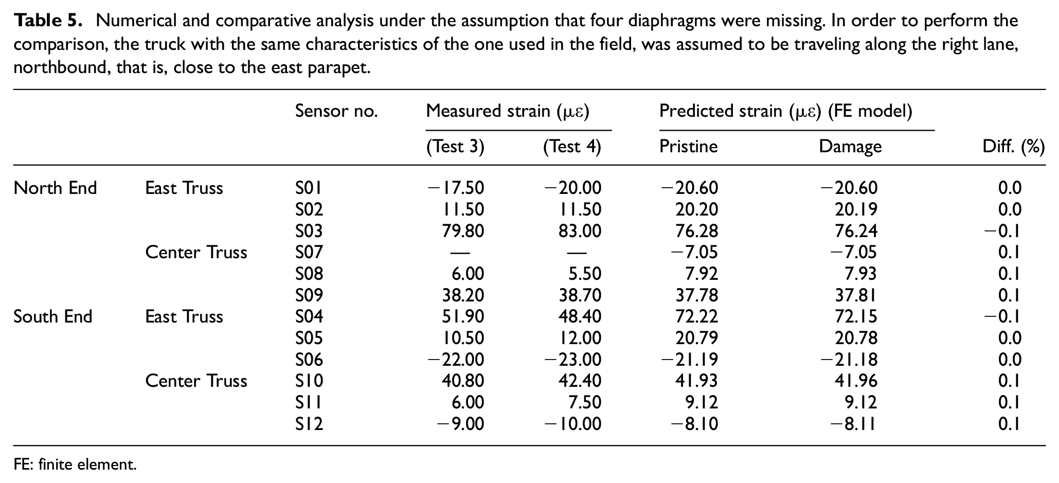
FE: finite element.

Table 6.

Numerical and comparative analysis under the assumption that four diaphragms were missing. In order to perform the comparison, the truck with the same characteristics of the one used in the field, was assumed to be traveling along the left lane, southbound, that is, close to the center truss.

		Sensor no.	Measured strain (µε)		Predicted strain (µε) (FE model)
			(Test 7)	(Test 8)	Pristine	Damage	Diff. (%)
North End	West Truss	S13	−8.50	−8.25	−6.80	−6.79	−0.2
		S14	7.20	6.50	8.54	8.52	−0.2
		S15	33.70	32.30	33.06	32.93	−0.4
	Center Truss	S07	—	—	−12.14	−12.15	0.1
		S08	8.50	8.40	13.66	13.67	0.1
		S09	76.90	73.40	77.90	77.94	0.1
South End	West Truss	S16	29.70	29.20	32.88	32.74	−0.4
		S17	6.60	6.50	7.83	7.81	−0.2
		S18	−5.00	−5.50	−6.24	−6.23	−0.2
	Center Truss	S10	79.50	77.10	78.10	78.15	0.1
		S11	8.50	9.00	12.68	12.69	0.1
		S12	−11.00	−10.50	−11.24	−11.25	0.1

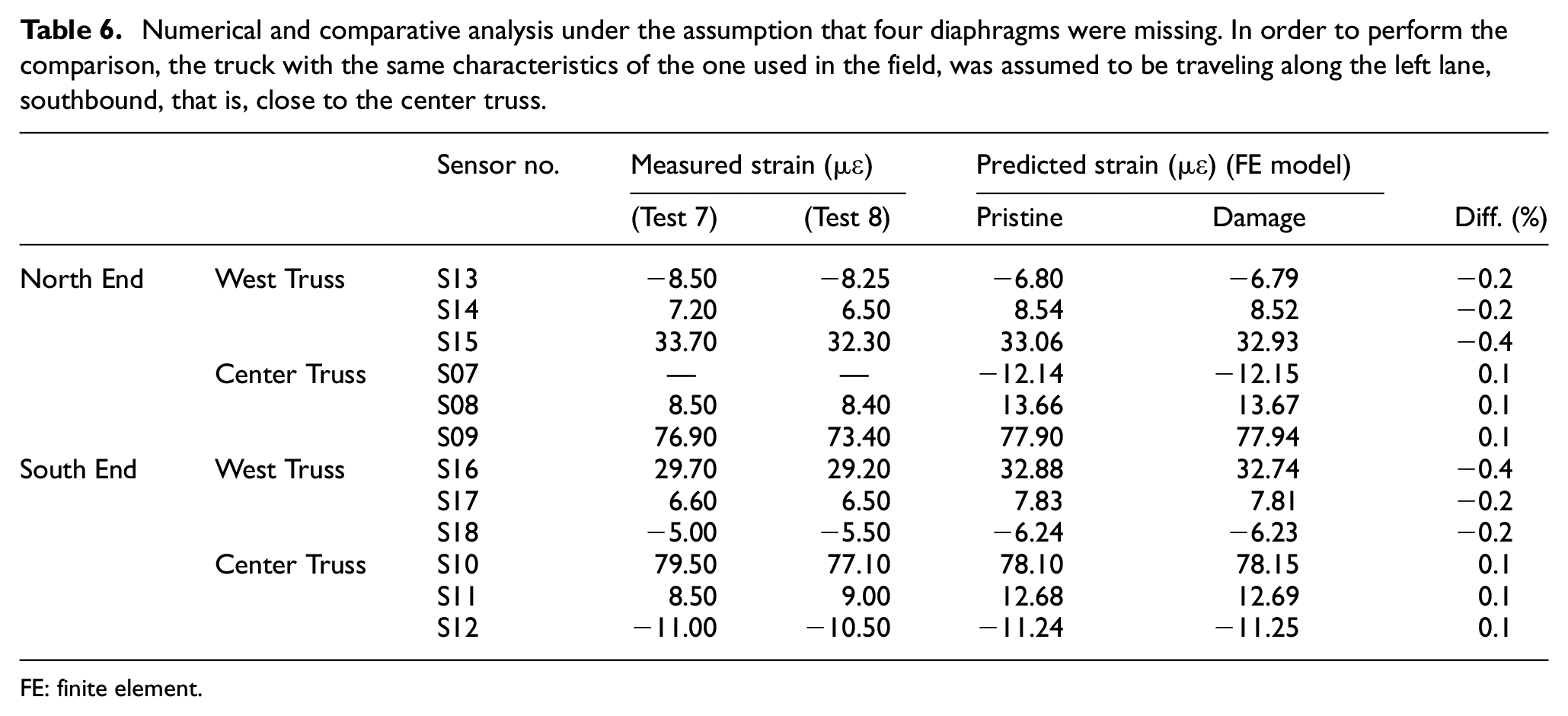
FE: finite element.

The second simulated damage was the removal of two diagonal bars, one from the center truss close to the south end and one from the west truss close to the north end (Figure 10). Tables 7 and 8 present the results and show that the simulated damage redistributes the load across the adjacent members. Thus, the installed sensors on the center truss (those that are close to south end) and the installed sensors on the west truss (those that are close to north end) show less strain.

Figure 10.

Damage scenario 2. A diagonal member close to (a) the north portal and (b) the south portal was removed.

Table 7.

Numerical and comparative analysis under the assumption that two diagonal members are missing. In order to perform the comparison, the truck with the same characteristics of the one used in the field, was assumed to be traveling along the right lane, northbound, that is, close to the east parapet.

		Sensor no.	Measured strain (µε)		Predicted strain (µε) (FE model)
			(Test 3)	(Test 4)	Pristine	Damage	Diff. (%)
North End	East Truss	S01	−17.50	−20.00	−20.60	−20.61	0.1
		S02	11.50	11.50	20.20	20.21	0.1
		S03	79.80	83.00	76.28	76.30	0.0
	Center Truss	S07	—	—	−7.05	−7.03	−0.2
		S08	6.00	5.50	7.92	7.91	−0.2
		S09	38.20	38.70	37.78	37.76	0.0
South End	East Truss	S04	51.90	48.40	72.22	72.89	0.9
		S05	10.50	12.00	20.79	20.90	0.5
		S06	−22.00	−23.00	−21.19	−21.30	0.5
	Center Truss	S10	40.80	42.40	41.93	40.67	−3.0
		S11	6.00	7.50	9.12	8.90	−2.3
		S12	−9.00	−10.00	−8.10	−7.92	−2.3

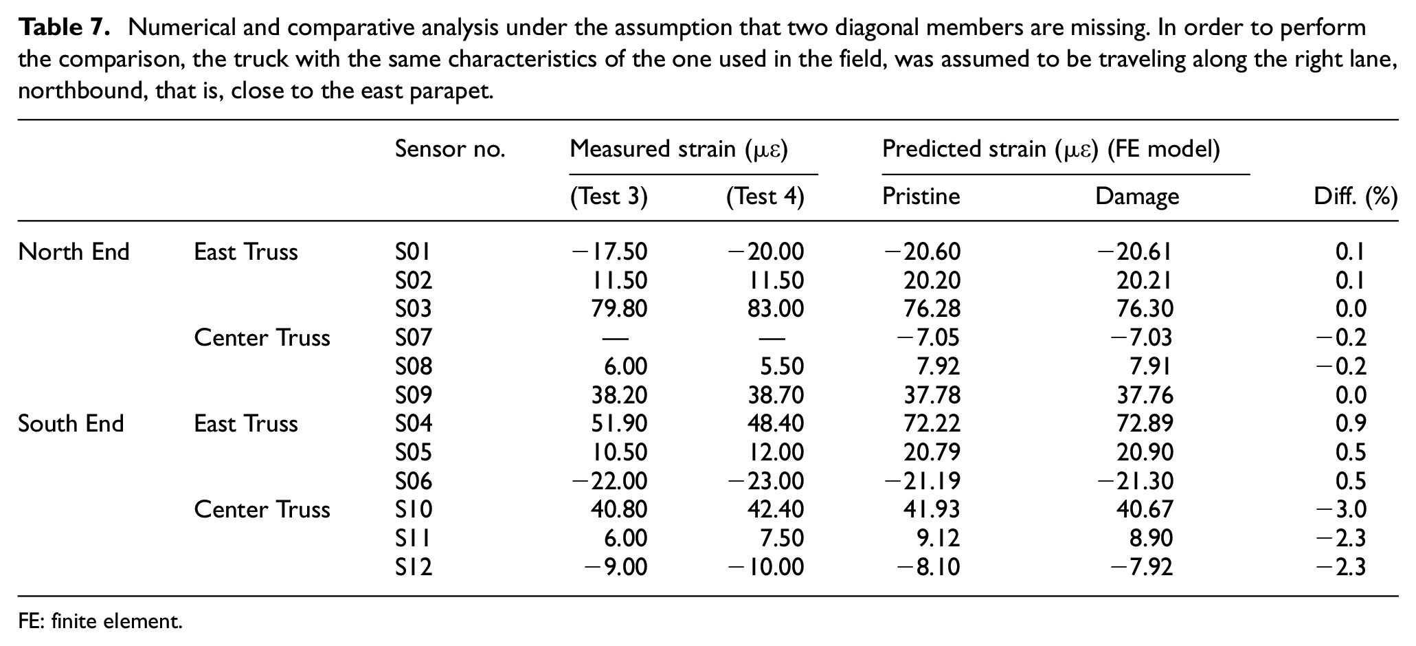
FE: finite element.

Table 8.

Numerical and comparative analysis under the assumption that two diagonal members are missing. In order to perform the comparison, the truck with the same characteristics of the one used in the field, was assumed to be traveling along the left lane, southbound, that is, close to the center truss.

		Sensor no.	Measured strain (µε)		Predicted strain (µε) (FE model)
			(Test 7)	(Test 8)	Pristine	Damage	Diff. (%)
North End	West Truss	S13	−8.50	−8.25	−6.80	−6.71	−1.3
		S14	7.20	6.50	8.54	8.42	−1.4
		S15	33.70	32.30	33.06	32.47	−1.8
	Center Truss	S07	—	—	−12.14	−12.18	0.3
		S08	8.50	8.40	13.66	13.71	0.3
		S09	76.90	73.40	77.90	78.44	0.7
South End	West Truss	S16	29.70	29.20	32.88	33.89	3.1
		S17	6.60	6.50	7.83	7.95	1.5
		S18	−5.00	−5.50	−6.24	−6.33	1.5
	Center Truss	S10	79.50	77.10	78.10	76.13	−2.5
		S11	8.50	9.00	12.68	12.36	−2.6
		S12	−11.00	−10.50	−11.24	−10.96	−2.5

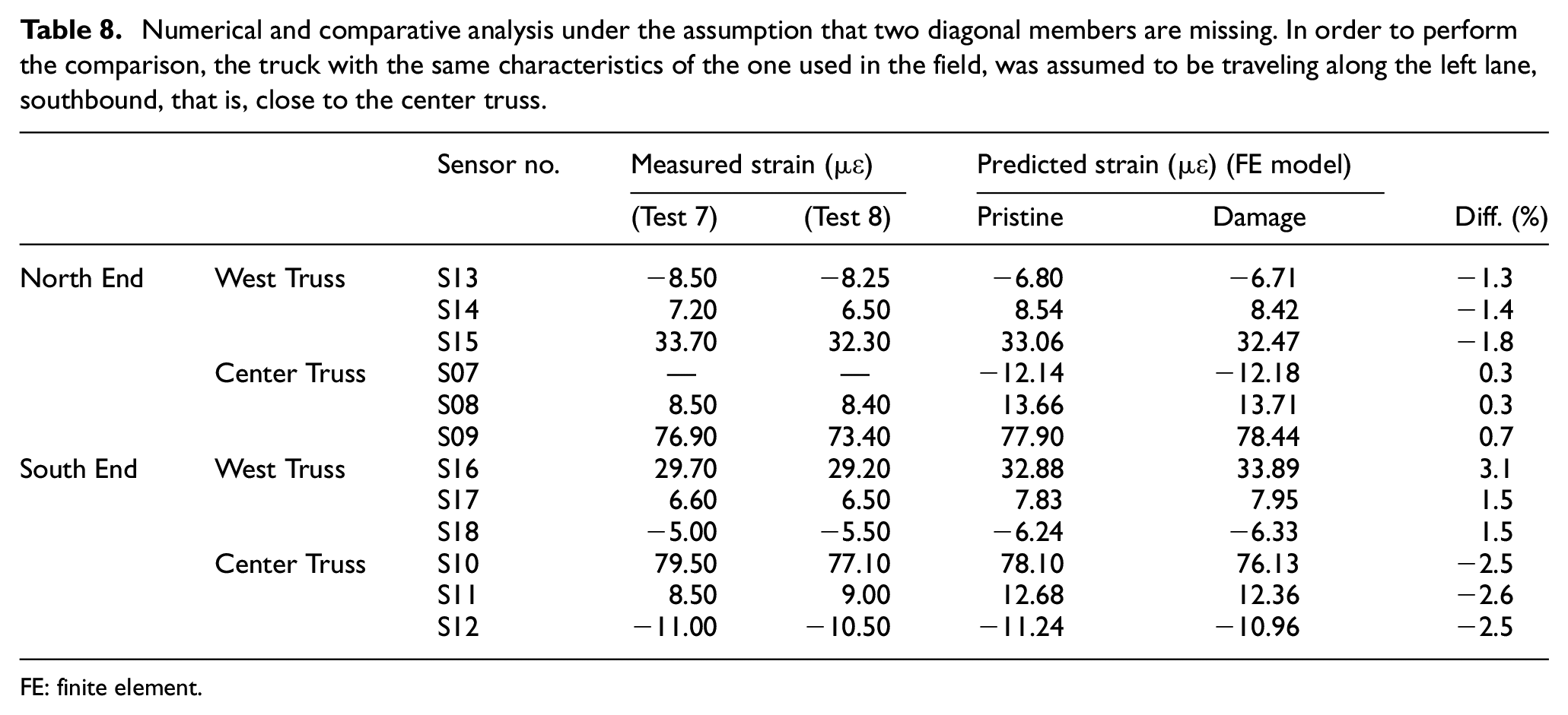
FE: finite element.

SHM algorithms

The data from the 18 strain gages were processed using a general framework designed by the authors and implemented in MATLAB software. The framework aimed to: (1) leverage the bridge response to thermal load in order to identify element-to-element differences that could be symptomatic of structural anomalies; (2) separate thermal effects from live load effects in order to capture transient events attributable to the crossing of heavy trucks, vehicle impacts, or barge collisions; (3) identify sensor drift. The framework was proven validated first by processing the data relative to the truckload test. Then, 3 years (August 1st, 2019 through July 31st, 2022) worth of data were examined. It is noted here that at the time of this paper submission, the SHM system was still active.

Algorithm validation: truckload test

Figure 11 shows the raw strains recorded during the truck test. The experiment lasted about 90 min during which the steel cooled about 3°C (5.5°F). From top to bottom, the values relative to the east, center, and west trusses are displayed. To ease comparison, the range of the vertical axes is identical. The values of the measured strains are not necessarily similar across symmetric elements, for example, S04 and S16, because the sensors were installed at different moments, when the temperature of the steel may have differed by more than 10°C. The consequence is that the raw strains are offset with respect to each other because the “reference temperature,” that is, the temperature at which the gages read zero deformation, is not the same for all the sensors. In addition, the temperature of the steel was not uniform. For example, the temperatures measured by S02 and S06 at 9 PM were equal to 27.1 and 24.7°C, respectively.

Figure 11.

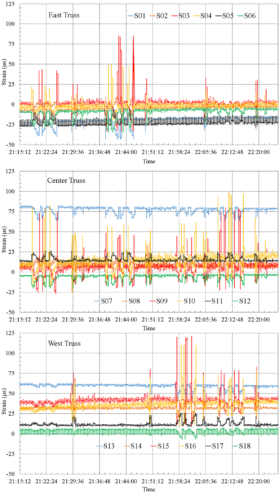
Raw strain measured during the truck test.

To minimize or eliminate any bias attributable to the temperature, the following three-steps procedure was implemented. First, the raw strain data and the raw temperature data were synchronized by up-sampling and interpolating the temperature data. Then, the 15-min moving average for both parameters was calculated. Finally, the difference between the raw and the moving averaged strain was calculated to obtain what hereinafter is referred to as the “true strain.” The hypothesis behind such procedure is that the effect of any transient event, for example, vehicle overload, vehicle crashes, or barge collisions, lasts much less than 15 min and therefore its effect on the moving average of the strain is negligible. Meantime, the inertia of the steel is such that the deformation induced by the temperature takes longer than 15 min. It is noted here that some authors³⁸ have considered longer intervals (60 min) to perform the moving average. The reliability of this procedure was applied to the data shown in Figure 11. The true strains relative to the sensors bonded to the center and the west trusses are presented in Figure 12. Here, the vertical axes are between −40 and +100 µε. In the absence of any live load, each value is centered to zero. Overall, the strain increments observed in Figure 12 are consistent with the maximum strain increases reported by the Vendor during the truck load test and schematized in Figure 4. The highest deformation was recorded by S09 and S10 bonded to the two control members. Figure 12 also confirms that the top chords monitored with sensors 07, 12, 13 and 18 are under compression.

Figure 12.

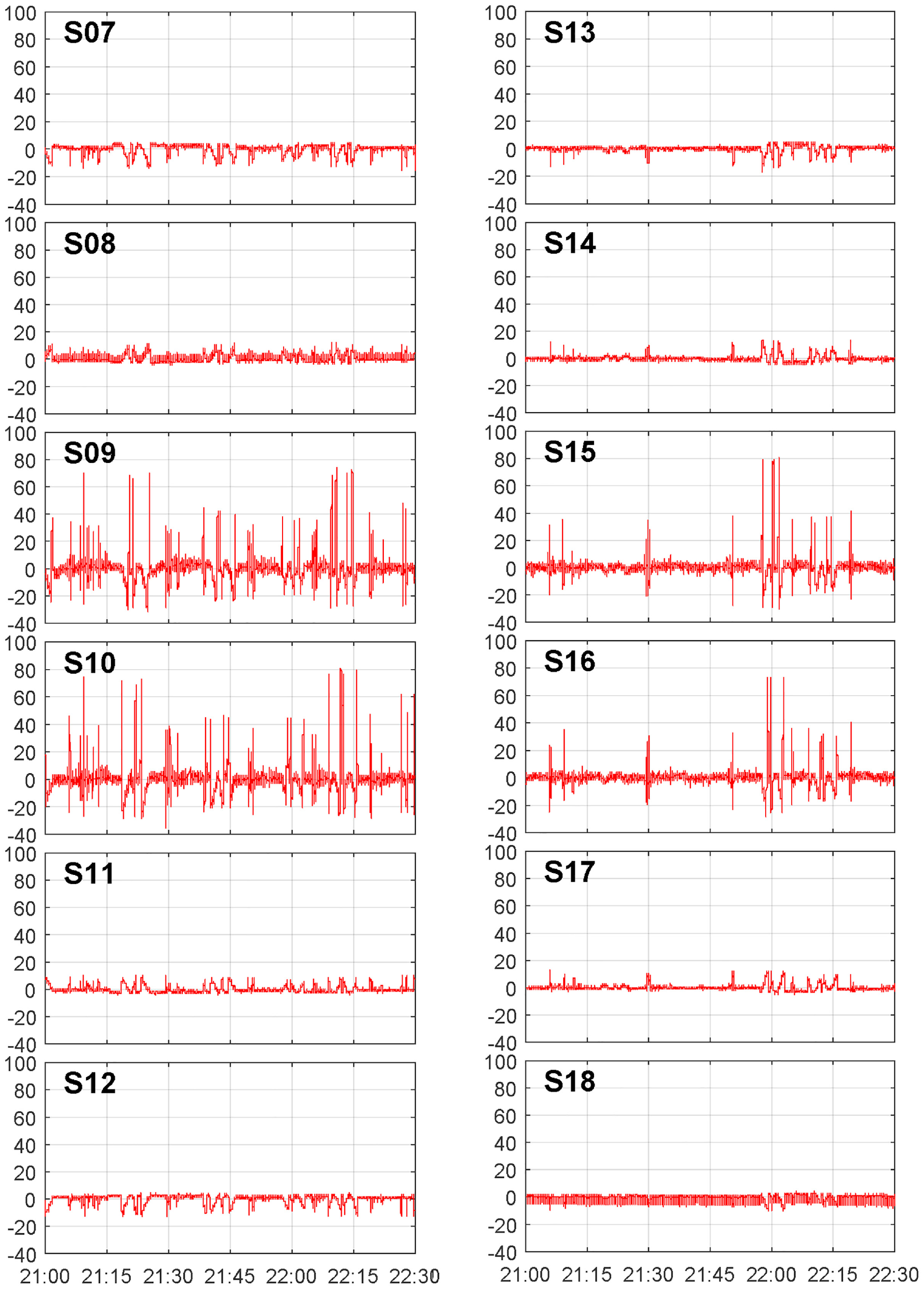
True strains from gages S08 to S18 extracted from the raw strains stored during the controlled load truck test. (The values on the vertical axes indicate strains and are expressed in microstrains.)

The effectiveness of the three-steps procedure described above is demonstrated further with Figure 13, which shows the data recorded by S16 during July 19–23 of year 2020. The steel temperature and the corresponding moving average are presented in Figure 13(a) and they overlap because metal heating or cooling takes longer than 15 min. The raw strains and the corresponding moving average are presented instead in Figure 13(b). The moving average is clearly tied to the temperature trend. The decrease of the temperature increases the strain and vice versa. The raw strains are instead a combination of traffic and thermal load. The difference between the two, that is, the true strain, is presented in Figure 13(c). Besides the fact that the absence of traffic is seen in the early hours of each day, Figure 13(c) shows a peak (152 µε) in the early morning of July 21, 2020. The value of 152 µε is nearly twice as that of any strain seen during the truck load test (Figure 12), and was triggered by the crossing of a very heavy truck traveling southbound. The FE model predicts that the expected static strain caused by a ML-80 type truck standing close to the south portal on the right southbound lane would be 102.1 µε. If a factor of 1.28 is used to account for the dynamic load of the moving truck traveling southbound, the resulting value of 131 µε (=102.1 × 1.28) is close to the measured deformation of 152 µε.

Figure 13.

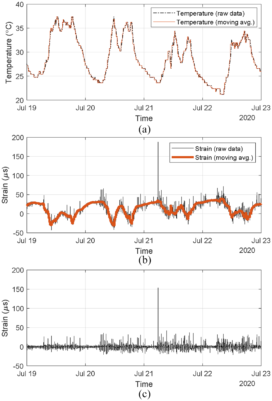
Mitigation strategy to isolate transient events: (a) Top: Raw and 15-min moving average of the temperature data, (b) Center: Raw and 15-min moving average of the strain data, and (c) Bottom: Live load strain.

From graphs like Figures 12 and 13(c), the average value (typically ∼0 µε) and the standard deviation σ can be extracted. Choosing an interval equal to 4σ, we can label as bridge overloads all those events that occur 0.0063% of the cases, that is, one case over 15,787 events. The selection of 4σ as threshold is arbitrary and based on statistical considerations. It can be replaced by a threshold based on engineering judgement such as traffic tonnage or numerical calculations such as those presented in section “The FE model.” For example, for the specific case of sensor 16, the threshold could be set equal to 72 × 1.28 (=92.16) µε, which is the static strain increase recorded in the diagonal member 16 when the 26,308 kg (58 kip) truck crawled over the southbound lane close to the parapet multiplied moving effects.

Long-term monitoring

This section discusses the outcome of the analyses of 3 years (August 1, 2019 to July 31, 2022) of active monitoring.

Raw data analysis

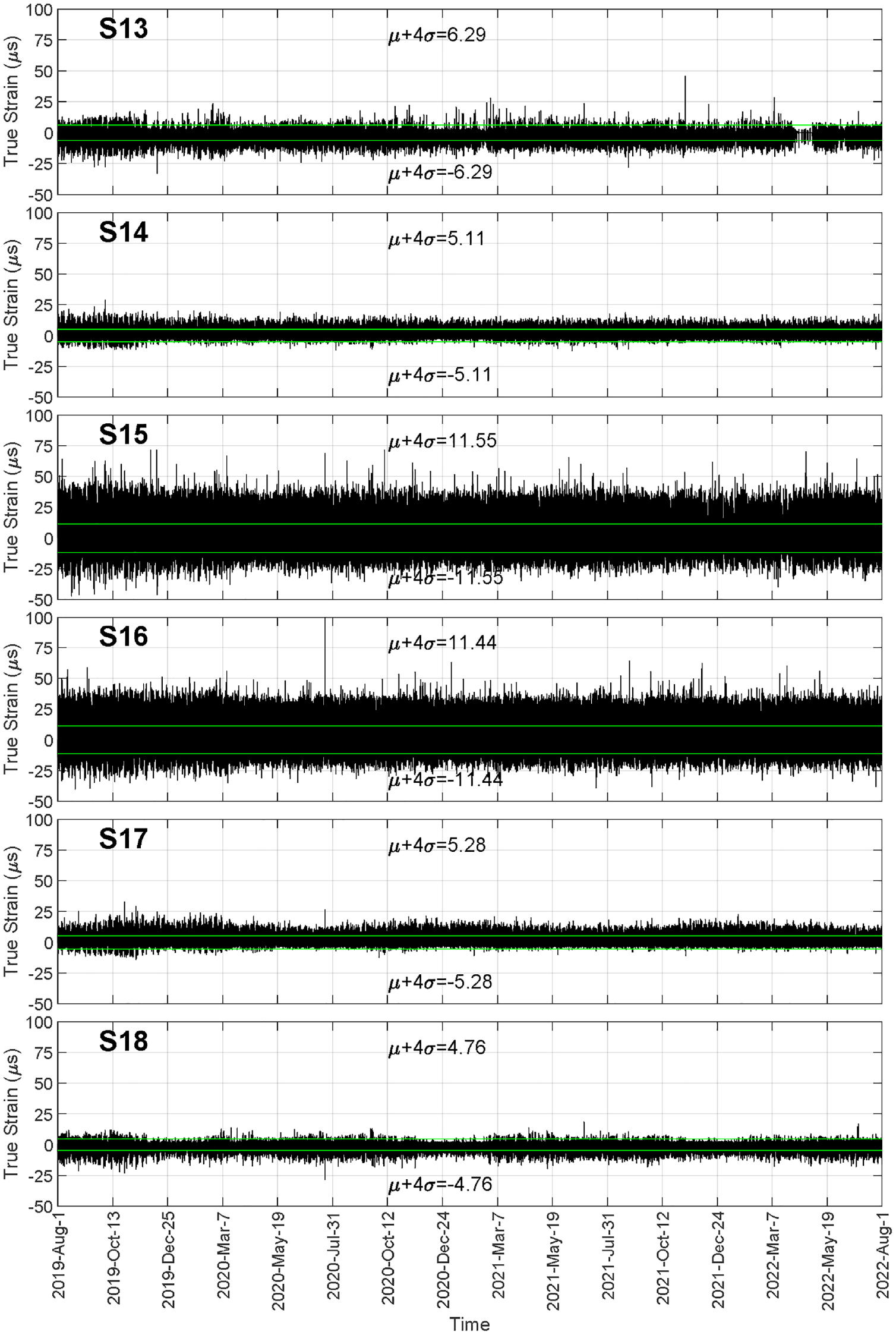
Figure 14 shows the raw strain and the corresponding 15-min moving average of gages S13 through S18. The two horizontal lines identify the ±4σ range. To facilitate data comparison, the vertical scale is identical and comprised between −150 and 200 µε, equivalent to −30–40 MPa if E = 200 GPa. For the sake of space, the graphs relative to the other 12 gages are not reported here but the following overall considerations are made:

Most deformations follow the seasonal changes of the temperature. This is particularly evident for the diagonal member monitored by gage S16.

Sensors S14 and S15 do not exhibit significant periodicity.

The width of the ±4σ range is not the same for all the sensors. While some ranges are below 50 µε (S02, S05), other gages (S01, S07, S13, S16) have ±4σ range wider than 150 µε. This is another indication that some members are less prone to thermal expansion/contraction. Among the less thermally prone members, thousands of deformations were outside the ±4σ interval. These are false positives, suggesting that the width of this interval is too sensitive for certain structural elements and therefore ineffective at identifying overloads or other transient events.

Only one isolated peak exceeded the ±4σ range and it was caused by the truck crossing discussed in section “Algorithm validation: truckload test.” Not shown here, other spikes were recorded by S04 on February 14, 2020 at 9:15:48 AM, and by S10 on July 22, 2021 at 15:21:02.

Figure 14.

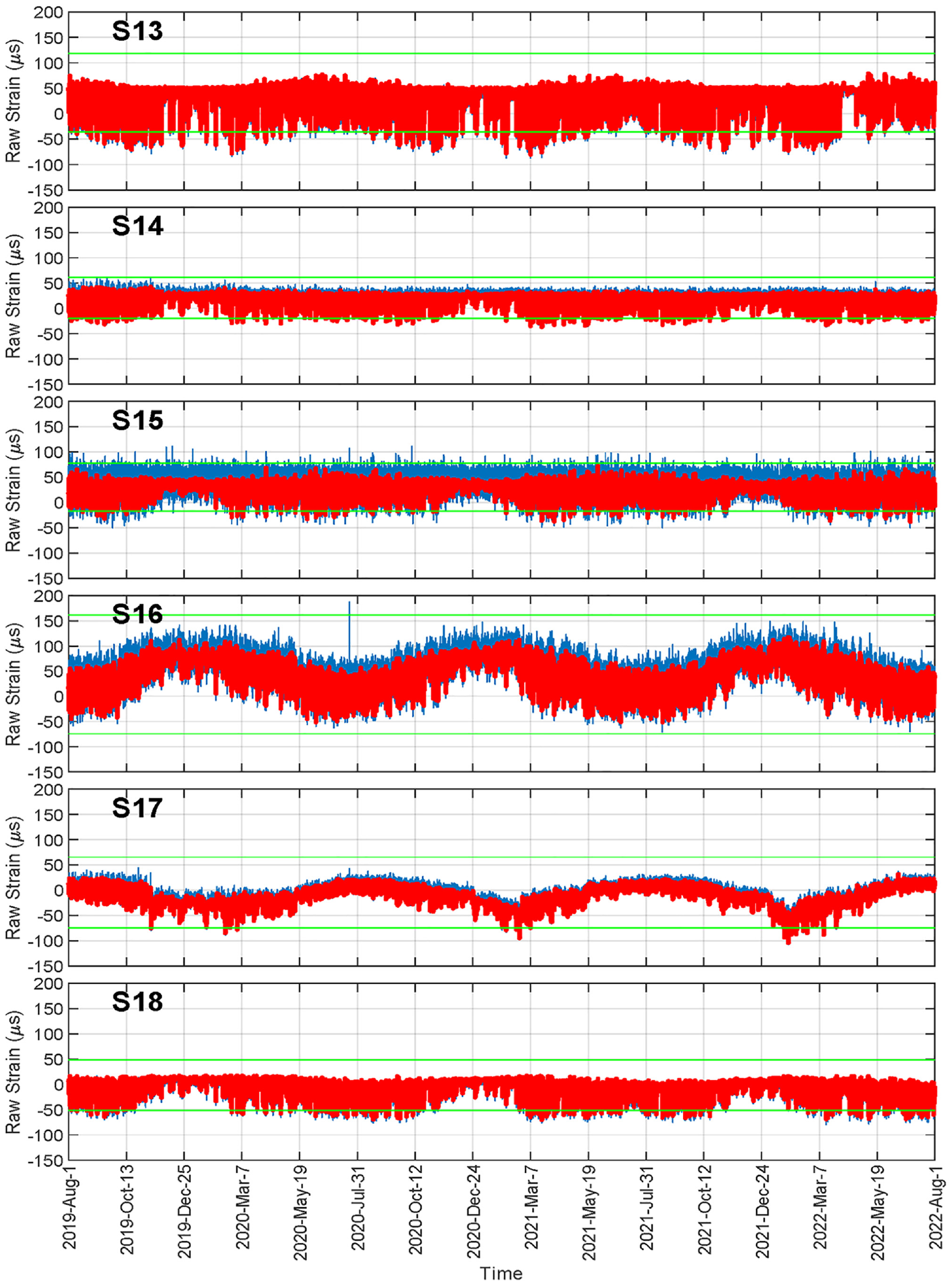
Raw strain and corresponding moving average recorded by six sensors over 3 years.

Graphs like Figure 14 can enable the identification of permanent deformation, and sensor drift. To date, nothing significant has emerged from the raw strains measured by the 18 sensors.

Thermal effects

The raw strains and the corresponding raw temperatures from each sensor were synchronized to create a matrix with three columns: strain, temperature, and corresponding timestamp. The temperatures and the corresponding strains are plotted in Figure 15 for the same gages considered in Figure 14. Each graph contains the lines bounding the ±4σ interval. The linear regression of the experimental data is overlapped (thick red line) and its equation and the corresponding R² are displayed. If any given member of the trusses is free to expand/contract, the slope of the equation would represent the coefficients of linear thermal expansion of the steel.

Figure 15.

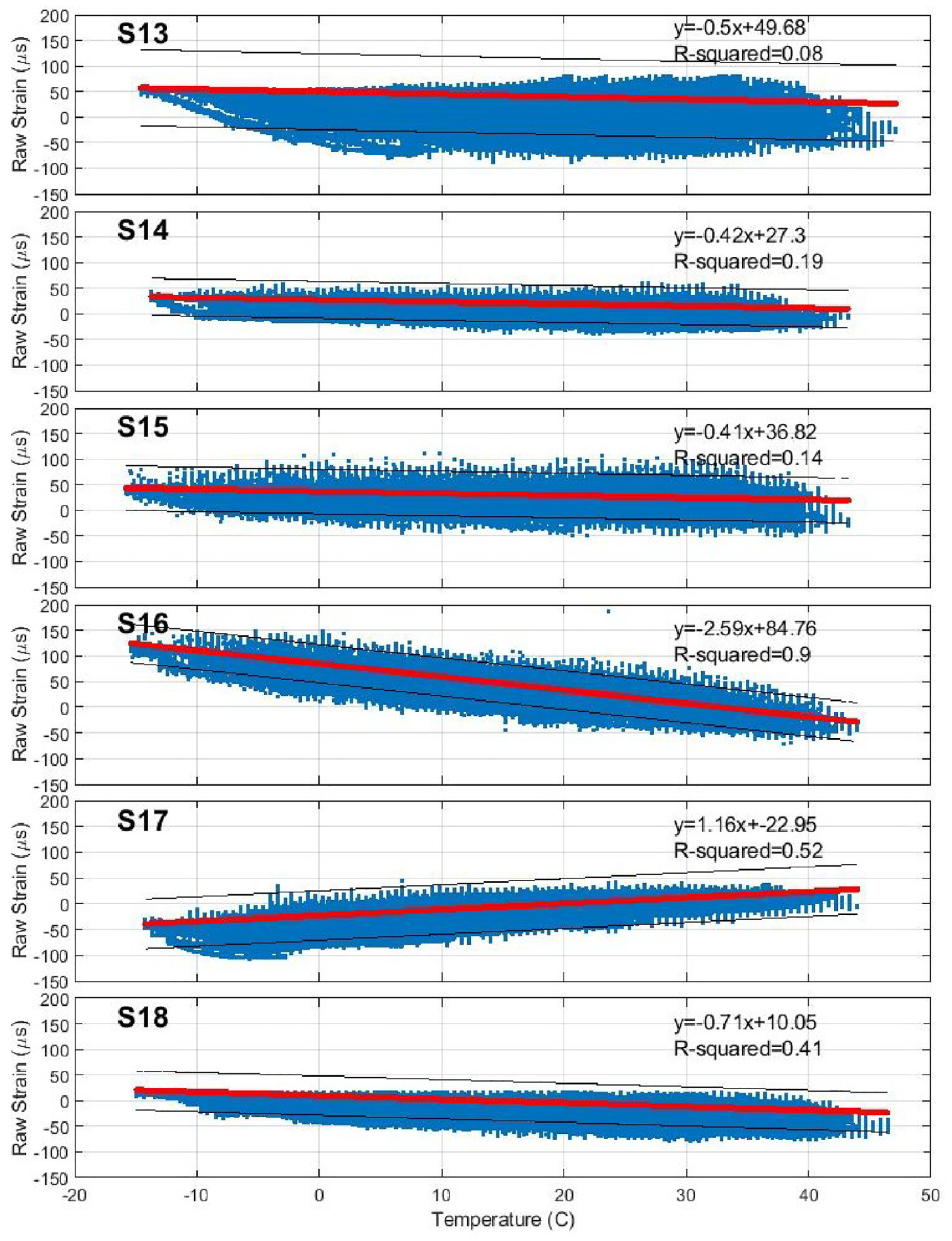
Raw strain vs raw temperature recorded by six strain gages over the 3 years monitoring period considered in this study.

With the exception of sensor S17, the deformation decreases with the increase of the temperature, that is, as the bridge becomes warmer its structural members tend to compress. The response of S17 is believed to be caused by the inversion of the gage terminals. This hypothesis could not be confirmed as the authors do not have access to the SHM system and to the Vendor. However, the error does not compromise the reliability of the information. The plots confirm the presence of the offset discussed in the first paragraph of section “Algorithm validation: truckload test.”

The crossing of the heavy truck discussed in section “Algorithm validation: truckload test” emerges with the dot close to 200 µε and 21°C (gage S16).

The slope for each sensor is presented in Figure 16(a) and visualized on the bridge schematics of Figure 16(b). Consistent with the presence of an expansion joint at the south end of Span 4, eight of the nine slopes calculated from the sensors bonded on the south end of the bridge are higher than the corresponding slopes from the north end. The only exception is S12, for which the value of −0.34 µε/°C is smaller than the slope calculated for gage S07 (−0.53 µε/°C). The strain gradients across the nine monitored members located on the north end are nearly the same. The only relevant exception is the diagonal member of the center truss, that is, gage S09. It is interesting to note that the slope at S04 is 51% the value of S16 (−1.32 µε/°C vs −2.59 µε/°C), and 40% the value of S10 (−1.32 µε/°C vs −3.32 µε/°C). Notably, the slope associated with S10 (−3.32 µε/°C) is nearly 20-fold the value calculated for S09 (−0.17 µε/°C). Such difference is not seen in any other pair. Finally, the cross comparison of the bottom south east and west chord suggests that the west chord expands more than its east counterpart, despite the cross-section of the latter being smaller.

Figure 16.

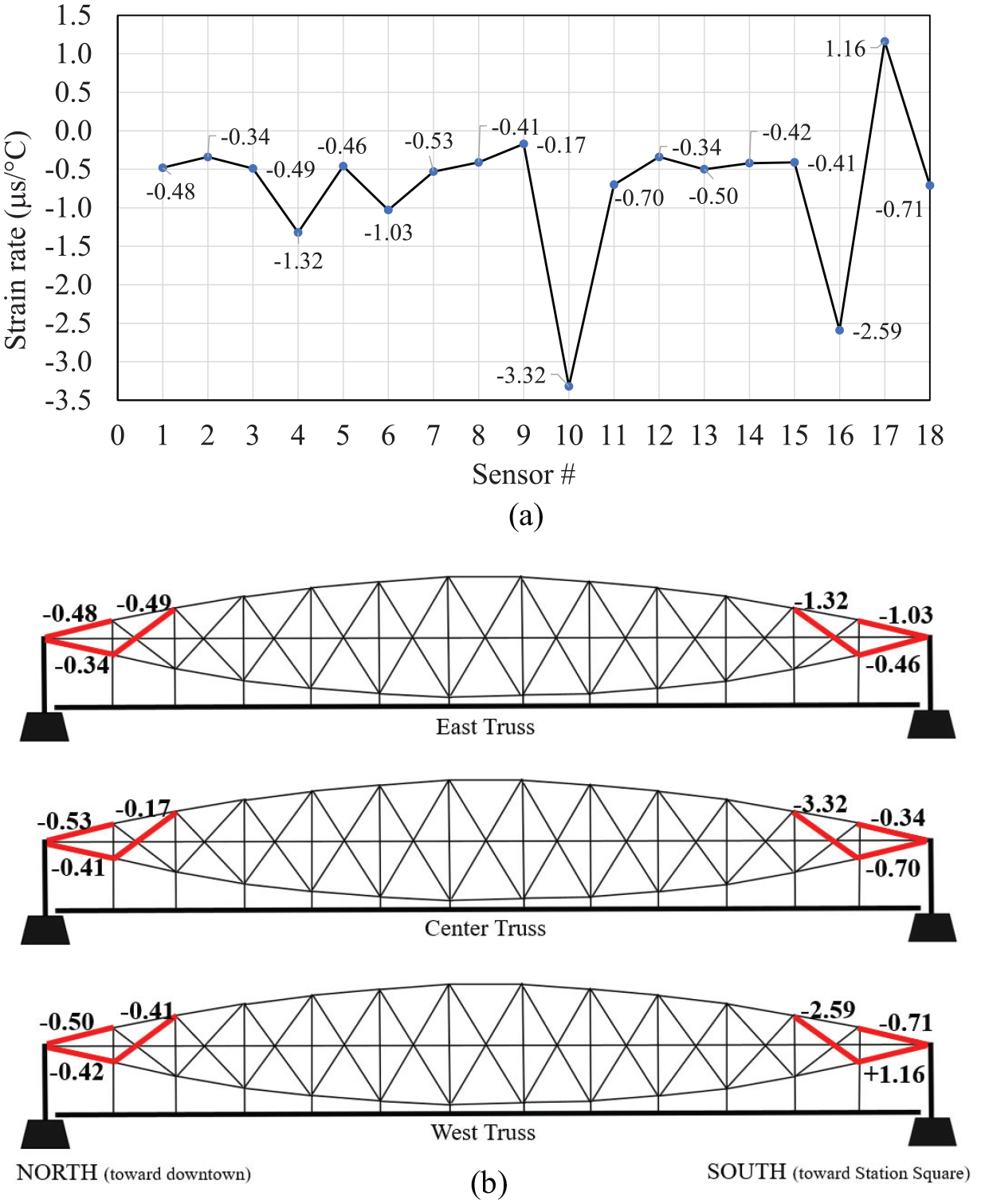
(a) Strain-temperature rate extracted from the sensors data over the 3 years monitoring period and (b) drawings of the east, center and west truss with the members instrumented and the corresponding strain rate expressed in µε/°C.

Figure 17 presents the R² of the line interpolations presented in Figure 15. The graph proves that the three single diagonal elements on the south side of the bridge, which is free to expand, respond linearly to the temperature variation as can be concluded by observing that the corresponding R² are close to 0.9. As expected, all the sensors bonded to the north side of Span 4, which cannot expand, exhibit the lowest R².

Figure 17.

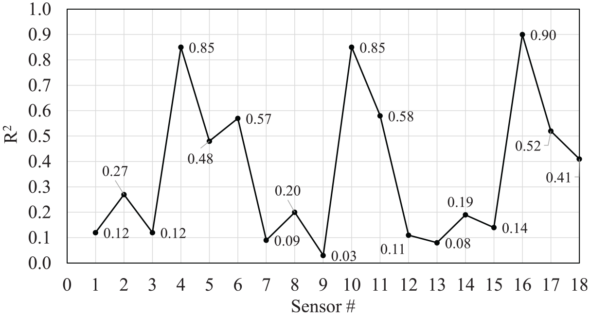
Residual R² of the linear interpolation of the strain vs temperature graphs.

The cross-comparison of graphs like Figures 15 to 17 can reveal anomalies with respect to thermal load. Based on what observed through Figure 14 to 17, it may be argued that the bridge does not respond symmetrically with respect to the median line and does not respond symmetrically with respect to the mid-span. The bottom chord on the south side of the west truss (S17) stands out from the other chords. The diagonal member on the south side of the East truss monitored with gage S04 seems to be partially locked as it does not exhibit the same gradient of the other two counterparts.

Live load effects

The “true strains” represent an accurate quantification of the deformation triggered by the live loads. An example of live load for a subset of strain gages is presented in Figure 18 along with two horizontal lines that bound the ±4σ range. To ease data comparison, the vertical scale is identical for all six graphs and comprised between −50 and 100 µε. Under the assumption that E = 200 GPa, the selected range goes from 10 MPa in compression to 20 MPa in tension. The true strains are consistent with what is seen with the truck load test (see Figure 12): the gages that exhibited small deformations (<20 µε) still showed small deformation over the last 3 years; the sensors (03, 04, 09, 10, 15, and 16) that exhibited an increase in strain above 50 µε instead showed high values of strains. On a few occasions, the sensors exceeded the maximum strain increase recorded during the truck test. Sensor S13 was subjected to an isolated event in November 2021 when the true stain was nearly 50 µε, significantly higher than the values typically recorded by this sensor. Gage S15 displays several isolated events, the most notable ones in December 2019, October 2020, and April 2022. Gage S16 displays a single spike much higher than 100 µε (151 µε), on July 21st, 2020, which is relative to the heavy truck crossing discussed previously. As observed for the raw strains, the selection of the ±4σ range may be too sensitive to identify relevant transient events. Perhaps a more appropriate marker could be the numerical values extracted from the static analysis presented in section “The FE model.”

Figure 18.

True strain extracted from gages S13 to S18 relative to the monitoring range August 2019 through July 2022. The 4σ interval is overlapped.

The values of the ±4σ range are presented in Figure 19. The graph corroborates what was found during the controlled truck test. The members that exhibited very small strain increase (see Figure 4 and 12) have the smallest range. This is a further proof of the reliability of the algorithm developed to extract the information about live loads. The analysis of the true strains shall not ignore the traffic pattern. The south portal of the bridge is located on an expansion joint but is also at a short distance from a traffic light. Vehicles traveling northbound are approaching the bridge after a 90° turn and therefore accelerate and reach full speed when approaching the north end of Span 4. Vehicles traveling southbound begin deceleration and breaking as they approach the traffic light and the 90° right or left turns become more visible. This implies that members instrumented with sensors S16–S18 are more likely to be subjected to the dynamic impact of traffic. Conversely, the members instrumented with sensors S04–S06 (east truss) are subjected to smaller dynamic loads because the vehicles heading northbound are slower and may begin accelerating. This may be the reason why the true strain graphs associated with some sensors may result in being noisier than others. Note that the controlled truck test was conducted at constant speed 8 km/h (5 mph) regardless of the traveling direction.

Figure 19.

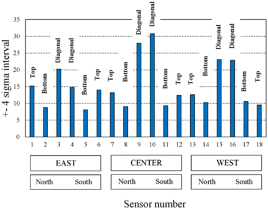
Value of the 4σ interval in µε calculated for each strain gage on the truss.

The analyses of Figures 18 and 19, including the 12 sensors not displayed here, led to the following considerations:

The true strains relative to sensors 02, 06, 08, 12, 14, and 18 do not reveal anything significant. Owing to its geometry, it is reasonable to believe that the strains at the top chord are in between the bottom and the diagonal members.

The amplitudes recorded by S17 (west truss) were significantly higher than sensors S05 and S11 bonded to the other bottom chords on the south side. This could be due to vehicles’ decelerations or to issues with the bridge bearings.

The sensor on the diagonal member of the east truss (S04) showed much lower amplitude than S10 and S16 bonded to the other two diagonal members of the south side. This evidence may support the hypothesis that the vehicles close to the south end of the bridge and traveling northbound are slower than those traveling southbound. An isolated event was detected around mid-February 2020 with a value close to the maximum strain of 51.9 µε recorded during the truck test. Sensor S10 at the center truss is mostly skewed to tensile stress with some events close to the value of 79.5 µε recorded during the truck test. This sensor recorded a significant negative strain (−395 µε) on July 22nd, 2022 at 15:21:02. Since it was only a single data point, not seen by any other gage, it is attributed to an electromagnetic interference. Sensor S16 detected a major event on July 21st, 2020 with a peak that is twice the value of 72.1 µε recorded during the truck test.

The comparison of the sensors located on the center truss did not reveal any specific trend. Owing to their location, any peak may be the result of the simultaneous crossing of two vehicles along the opposite directions.

The value of the ±4σ interval displayed in Figure 19 may also provide a qualitative estimate of the responsiveness of each sensor and of the proper elongation/contraction of the relative bridge element. Figure 19 shows that the individual diagonal members experienced the largest strain variation. The exception is the top member located on the north side of the east truss (S01). Conversely, the bottom chords seem to be the most rigid with least strain variation. Overall, the behavior observed with Figure 19 is compatible to the geometry of the 18 members being monitored: the slender elements exhibit the largest interval, whereas the bulkiest part (the bottom chords) exhibits the smallest interval. The outlier represented by the information collected with S01 may be related to the installation of the sensor far from the neutral axis, that is, the sensor may read flexural strain besides axial strain.

Outlier analysis

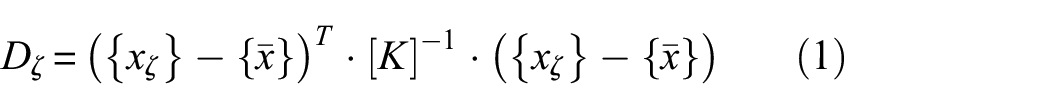
OA is a novelty detection method that establishes whether a new configuration of a given system is discordant or inconsistent from the baseline configuration, which consists of an existing set of data (or patterns) that describes the normal operative conditions. Ideally, if the OA is used for damage detection, the baseline should include normal variations in environmental or operative conditions of the structure (e.g., temperature, humidity, loads). In this study, multivariate OA was performed by computing the Mahalanobis squared distance (MSD) D_ζ, which is a scalar defined as^12–14:

D_{ζ} = {({x_{ζ}} - {\bar{x}})}^{T} \cdot {[K]}^{- 1} \cdot ({x_{ζ}} - {\bar{x}})

(1)

was calculated. In Equation (1), {x_ζ} is the potential outlier vector, ${\bar{x}}$ is the mean vector of the baseline, [K] is the covariance matrix of the baseline and T is the transpose symbol. The baseline mean vector and the covariance matrix were calculated exclusively without contaminating the statistics of the baseline data.

In order to determine whether a new datum is an outlier, the corresponding D_ζ has to be compared to a threshold computed from the baseline. Usually, the baseline data set consists of a large number of samples collected under all possible environmental conditions. Once the values D_ζ of the baseline distribution are determined, the threshold value is typically taken as the upper value of 3σ, equal to 99.73% of the Gaussian confidence limit. Thus, if a new datum was classified as an outlier, theoretically there is only a 0.27% chance of a “false positive” reading. This approach assumes that the samples sufficiently represent the statistical distribution as a Gaussian curve.

In this study, each truss was considered individually. As such, the input vector contains the true strains from six sensors. The baseline consisted of all the data collected during the month of August 2019. This relatively short interval was deemed to be representative of the baseline because the OA was applied to the true strains, and the true strains are unbiased by thermal effect. The threshold was instead set as the upper value of 4σ. The results of the OA are presented in Figure 20. About 20 relevant outliers emerge and are indicated with date and times. The largest MSD (close to 10,000) was found at the center truss on July 22, 2021 and was caused by what is believed to be an electromagnetic interference. The second largest MSD (∼2000) was seen at the west truss on July 21, 2020 and is relative to the heavy truck crossings discussed previously. By looking at the date and hours, it was determined that these outliers were caused by the sensors bonded to the single elements of the bridge, that is, to the diagonal members.

Figure 20.

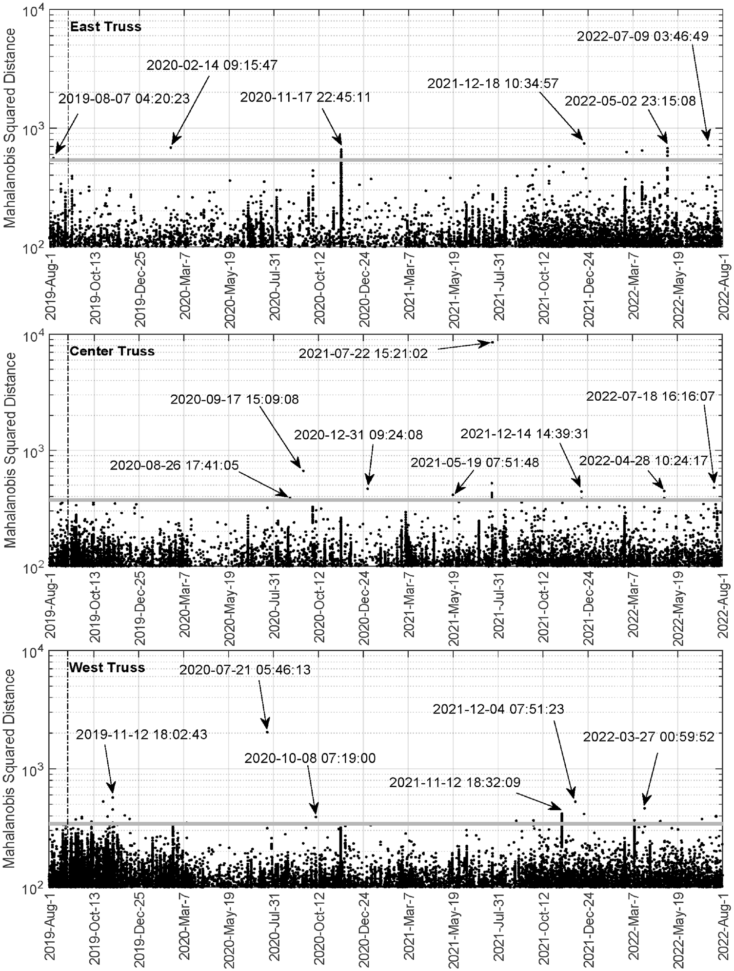
Mahalanobis squared distance applied to the strain gage data on the individual trusses. From top to bottom, east, center, and west truss.

Figure 20 shows the reliability of the analysis at identifying outliers of a certain significance. To this end, while the investigation of the outlier on July 22, 2021 in the center truss identified a false positive, the outlier on July 21, 2020 in the west truss revealed the passing of an overweight unauthorized truck over the bridge. In addition, the classification of the sensors into three groups (east, center, and west) may help the localization of any potential issues recorded by the sensors. For example, the outlier relative to the overweight truck is identified in the west truss analysis, which implies that the truck was traveling southbound, close to the parapet. It must be noted that the application of the OA presented here required some data prepping. Owing to sensors synchronization, the time stamp for each recording may not have been identical to each of the sensors included in a given cluster, that is, in a given truss. To overcome the lack of data synchronization, the pre-processing included the insertion of strain data that represented the linear interpolation between two consecutive recording.

The OA was also run for the time interval corresponding to the evening of the controlled truck load test. For the sake of space, the results are not shown here. However, it was found that most of the truck crossings resulted in several outliers slightly above the corresponding threshold of each truss.

Conclusion

This paper presented a comprehensive study about one of the most iconic bridges in the city of Pittsburgh, the Smithfield Street Bridge. The bridge was modeled using a commercial FE software to predict the deformation of those members that are currently monitored with wireless strain sensors that are part of a more comprehensive SHM system installed by a company not involved with the research presented here. The numerical deformations were calculated under the assumption that the bridge is subjected to the load of a truck of well-defined geometry and weight. Four different trucks were considered. One of these trucks was identical to the vehicle used by the private company to perform a truck load test. The experimental results of this test were compared with the numerical results predicted with the FE model and they showed very good agreement, despite uncertainties about the lateral distance of the truck from the centerline of the bridge. The study was then complemented with a thorough analysis of the SHM data made available to the authors. The effect of the temperature on the strains was exploited to identify any anomalous behavior of the members being monitored. In addition, a simple algorithm was then implemented to mitigate the effect of temperature in order to extract the deformation induced by traffic or other transient events (live loads). The strains from the live loads were then combined into an OA to detect anomalies that may be of significance for the bridge owner. Overall, it was observed that the south side of the west truss exhibits slightly larger thermal deformations than its east counterpart. The same truss shows slightly higher strains due to live loads. The motivation may be structural, but it may also be associated with differences in the number and speed of the vehicles traveling southbound. The live load graphs may reveal isolated peaks that can be attributed to heavy traffic or a sudden transient event of a different kind. These graphs enable the comparison with the value of the maximum strain recorded during controlled truck tests because the graphs are not adversely affected by the offset induced by the installation. However, live load graphs cannot reveal either sensors drift or permanent deterioration of the structure because the live load is obtained by subtracting the raw strain to the 15-min moving average.

Owing to the overall cross-sectional geometry of the monitored components, a direct comparison between the individual diagonal member and the top chord, which is formed by four I-shaped steel members riveted together, and between the diagonal member and the bottom chord, which is by bars pinned together, can only be approximate. In fact, the diagonal member is a single element carrying axial stress; the instrumented bottom chord is one of the eight bars designed to carry axial stress; the cross-section of the top chord is different from the other two. Future studies may look at the data from the other two kinds of sensors installed on the bridge, namely the displacement and the rotation sensors, and at analyzing new data. The strain gage sensors installed on the trusses are still active and are not showing any relevant issues, including drift. Future studies may also consider the inclusion of thermal effects into the numerical analyses.

Footnotes

Acknowledgements

The contents of this document are not meant to represent standards and are not intended for use as a reference in specifications, contracts, regulations, statutes, or any other legal document. The opinions and interpretations expressed are those of the authors and other duly referenced sources. The views and findings reported herein are solely those of the writers and not necessarily those of PennDOT. This paper does not constitute a standard, a specification, or regulations. The model presented here is based on drawings of the Bridge provided to the authors and may not necessarily reflect any modifications made over the years to rehabilitate/retrofit the structure. The second author performed this research while working under the supervision of the corresponding author. The FE data may be made available upon reasonable requests. The availability of the raw strain data may require special permission from the research sponsor.

Declaration of conflicting interests

The author(s) declared no potential conflicts of interest with respect to the research, authorship, and/or publication of this article.

Funding

The author(s) disclosed receipt of the following financial support for the research, authorship, and/or publication of this article: The authors acknowledge the support of the Pennsylvania Department of Transportation (PennDOT) under contract 4400018535, PIT WO 003 titled “Data Management, Mining, and Inference for Bridge Monitoring.”

ORCID iD

Piervincenzo Rizzo

References

Federal Highway Administration, https://www.fhwa.dot.gov/bridge/nbi/ascii.cfm (2019).

Pennsylvania Department of Transportation, https://www.penndot.pa.gov/ProjectAndPrograms/Bridges/Pages/Bridge-Inspection-Terminology.aspx (accessed 3 October 2023).

Federal Highway Administration, https://www.fhwa.dot.gov/bridge/britab.cfm (accessed 3 October 2023).

Federal Highway Administration, https://www.federalregister.gov/documents/2017/01/18/2017-00550/national-performance-management-measures-assessing-pavement-condition-for-the-national-highway (accessed 3 October 2023).

ASCE Report Card 2021, https://infrastructurereportcard.org/wp-content/uploads/2020/12/Bridges-2021.pdf (2021)

U.S. Department of Transportation, https://www.transportation.gov/testimony/highway-bridge-inspections (accessed 3 October 2023).

Glisic

. Concise historic overview of strain sensors used in the monitoring of civil structures: the first one hundred years. Sensors 2022; 22(6): 2397.

Barthorpe

Manson

Worden

. On multi-site damage identification using single-site training data. J Sound Vib 2017; 409: 43–64.

Worden

Manson

. The application of machine learning to structural health monitoring. Philos Trans R Soc London Ser A 2007; 365(1851): 515–537.

10.

Zhang

Sun

. Multi-site structural damage identification using a multi-label classification scheme of machine learning. Measurement 2020; 154: 107473.

11.

Ghahremani

Enshaeian

Rizzo

. Bridge health monitoring using strain data and high-fidelity finite element analysis. Sensors 2022; 22(14): 5172.

12.

Bagheri

Pistone

Rizzo

. Outlier analysis and artificial neural network for the noncontact nondestructive evaluation of immersed plates. Res Nondestr Eval 2015; 26(3): 154–173.

13.

Zheng

Rizzo

Nasrollahi

. Outlier analysis of nonlinear solitary waves for health monitoring applications. Struct Health Monit 2020; 19(4): 1160–1174.

14.

Rizzo

Sorrivi

Lanza

Scalea

, et al. Wavelet-based outlier analysis for guided wave structural monitoring: application to multi-wire strands. J Sound Vib 2007; 307(1–2): 52–68.

15.

Lanza

Scalea

Rizzo

Coccia

, et al. Non-contact ultrasonic inspection of rails and signal processing for automatic defect detection and classification. Insight 2005; 47(6): 346–353.

16.

Rizzo

Enshaeian

. Bridge health monitoring in the United States: a Review. Struct Monit Maint 2021; 8(1): 1–50.

17.

French

CEW

Shield

Hedegaard

. Modeling and monitoring the long-term behavior of post-tensioned concrete bridges. Report No. MN/RC 2014-39, Minnesota Department of Transportation, Minneapolis, 2014.

18.

Hedegaard

French

Shield

, et al. Instrumentation and modeling of I-35W St. Anthony Falls bridge. J Bridge Eng 2013; 18(6): 476–485.

19.

French

CEW

Shield

Stolarski

, et al. Instrumentation, monitoring, and modeling of the I-35W Bridge. Report No. MN/RC 2012-24, Minnesota Department of Transportation, Minneapolis, 2012.

20.

Gaebler

Hedegaard

Shield

, et al. Signal selection and analysis methodology of long-term vibration data from the I-35W St. Anthony Falls Bridge. Struct Control Health Monit 2018; 25(7): e2182.

21.

Hedegaard

French

Shield

. Time-dependent monitoring and modeling of I-35W St. Anthony Falls Bridge. I: analysis of monitoring data. J Bridge Eng 2017; 22(7): 04017025.

22.

Hedegaard

French

Shield

. Long-term monitoring strategy for time-dependent deflections of posttensioned concrete bridges. J Bridge Eng 2017; 22(11): 04017095.

23.

Shenton

III Al-Khateeb

Chajes

, et al. Indian river inlet bridge (part A): description of the bridge and the structural health monitoring system. Bridge Struct 2017; 13(1): 3–13.

24.

Shenton

III Chajes

Wenczel

, et al. Load tests of the Charles W. Cullen bridge at Indian river inlet. Technical Report, Center for Innovative Bridge Engineering, University of Delaware, Newark, Delaware, 2016.

25.

Shenton

III Chajes

Wenczel

, et al. Inaugural load test of the Charles W. Cullen bridge at Indian river inlet. Report No. DCT 238, Center for Innovative Bridge Engineering, University of Delaware, Newark, Delaware, 2013.

26.

Al-Khateeb

Shenton

III Chajes

, et al. Structural health monitoring of a cable-stayed bridge using regularly conducted diagnostic load tests. Front Built Environ 2019; 5(41): 1–12.

27.

Natalicchio

. Model calibration of the Indian River Inlet Bridge using structural health monitoring strain data. PhD Dissertation, University of Delaware, Newark, Delaware, 2018.

28.

. Structural health monitoring and model updating of Aizhai suspension bridge. J Aerosp Eng 2017; 30(2): B4016009-1-15.

29.

Schlune

Plos

Gylltoft

. Improved bridge evaluation through finite element model updating using static and dynamic measurements. Eng Struct 2009; 31(7): 1477–1485.

30.

Chen

. Finite element model updating of existing steel bridge based on structural health monitoring. J Cent South Univ Technol 2008; 15(3): 399–403.

31.

Duan

Fei

, et al. Advanced finite element model of Tsing Ma Bridge for structural health monitoring. Int J Struct Stab Dyn 2011; 11(2): 313–344.

32.

Gatti

. Structural health monitoring of an operational bridge: a case study. Eng Struct 2019; 195: 200–209.

33.

Schommer

Nguyen

Maas

, et al. Model updating for structural health monitoring using static and dynamic measurements. Procedia Eng 2017; 199: 2146–2153.

34.

Venuti

Domaneschi

Lizana

, et al. Finite element models of a benchmark footbridge. Appl Sci 2021; 11(19): 9024.

35.

Catbas

Susoy

Frangopol

. Structural health monitoring and reliability estimation: long span truss bridge application with environmental monitoring data. Eng Struct 2008; 30(9): 2347–2359.

36.

Kulcu

Qin

Barrish

JRA

, et al. Information technology and data management issues for health monitoring of the Commodore Barry Bridge. In: Proceedings of the SPIE’s 5th annual international symposium on nondestructive evaluation and health monitoring of aging infrastructure; SPIE-Intl Soc Optical Eng 2000, Newport Beach, CA, USA, pp. 98–111.

37.

Pines

Aktan

. Status of structural health monitoring of long-span bridges in the United States. Prog Struct Eng Mater 2002; 4(4): 372–380.

38.

Huang

, et al. New representative temperature for performance alarming of bridge expansion joints through temperature-displacement relationship. J Bridge Eng 2018; 23(7): 04018043.