
Abstract
Welding is a commonly used method for joining two or more parts together in steel construction. Various defects in weld regions such as cracks, pores, and slag inclusion can be present from the beginning, generated during the welding process, or can be developed while in service. Such defects are the weak spots that degrade the structure’s quality and can lead to structural failures. Therefore, early detection of these defects in welded joints, before visible cracks appear, is very important. Using appropriate ultrasonic non-destructive testing and evaluation (NDT&E) techniques, one can detect these defects and take remedial actions to prevent catastrophic structural failures. Guided acoustic wave-based techniques have been proven to be effective for damage detection in steel pipes and rods. Several studies have previously attempted to detect damage in steel tubes using guided ultrasonic waves. Unlike earlier attempts which mostly focused on conventional linear ultrasonic techniques, a relatively new nonlinear ultrasonic technique called sideband peak count-index (SPC-I) is carried out in this research. For this investigation, cast steel components and round hollow structural sections are welded together, and a four-point bending test is conducted under fatigue loading. The welded joints are continuously monitored in real time using strain gages and lead zirconate titanate (PZT) transducers. The PZT transducers are used to generate and receive guided acoustic waves. The signal is propagated through the specimen in a single-sided transmission mode setup. The strain gage readings and the nonlinear ultrasonic parameter, the SPC-I values, are monitored simultaneously. The results obtained from the nonlinear ultrasonic NDT&E measurements are compared with the data obtained from the strain gages to determine the robustness and reliability of the SPC-I technique for monitoring welded joints. This investigation also shows the potential effectiveness of the nonlinear ultrasonic parameter SPC-I for early detection of weld failure.
Keywords
Introduction
Structural steel is one of the most widely used construction materials because of its desirable properties—high strength, ductility, and constructability. Frequently, fabricated steel parts are delivered to the construction site and assembled. Welding is one of the two accepted joining methods in steel construction (along with bolting). However, the occurrence of defects such as cracks, pores, and slag inclusion in welded joints is inevitable. The defects may be present in the parent material and can arise due to the welding process as well. Heat-affected zone (HAZ) due to welding can also lead to weaker inherent material. Welding creates residual stresses, high triaxial restraint, and a HAZ with diminished properties. Welded joints are generally vulnerable to fatigue loading due to the presence of internal defects and weaknesses in HAZ which can result in structural failure. 1 Thus, controlling and monitoring the quality of the welded joints are critically important. One approach to inspect the welded joints is to take the help of ultrasonic non-destructive testing and evaluation (NDT&E) techniques. Ultrasonic testing is one of many techniques used in NDT&E industry today. In ultrasonic testing, any change in the ultrasonic wave transmitted through the material is monitored and analyzed to evaluate the condition of the material.
Most ultrasonic NDT&E techniques widely adopted in the industry are conventional linear ultrasonic techniques. Defects present in a material affect a signal passing through it. Thus, in principle, defects can be detected and characterized by analyzing the changes in received signals. The variations in linear ultrasonic parameters are generally noticeable for relatively large defects; however, it is often negligible and hence hardly detectable for very small defects such as microscale damage. Nonlinear ultrasonic techniques are known to be more sensitive to microscale damage compared to conventional linear ultrasonic techniques.2–6 One popular reason that causes the nonlinearity is the breathing effect (opening and closing) of microcracks. As waves propagate through a material, the opening and closing of microcracks create the changes in stiffness of the material with strain and time, which introduces material nonlinearity.7–10 It should be noted that such microcrack-induced nonlinearity can occur in the elastic range of the stress–strain relation of the material. Breathing cracks change elastic stiffness locally as those cracks open and close due to propagating elastic waves. The breathing microcracks cause nonlinear stress–strain behavior. Such small nonlinearity can be detected by nonlinear ultrasonic techniques even when the global stress–strain response shows almost a linear behavior under loading. It is because the microcrack-induced nonlinearity is so small that this small curvature in the stress–strain plot is difficult to detect through traditional stress–strain experiments.
Two well-established nonlinear ultrasonic techniques commonly used to evaluate material nonlinearity include (1) higher harmonic generation (HHG)9–28 and (2) nonlinear wave modulation spectroscopy (NWMS) or frequency modulation (FM).29–36 However, there are some challenges for practical field applications of these techniques. Certain conditions must be met to use the HHG technique properly, such as material homogeneity; the use of the same wave traveling path; and high voltage to increase the sensitivity of the technique. Moreover, when it comes to waveguides such as plates, pipes, and rods where the wave propagates as guided waves—Rayleigh surface wave and Lamb wave—the dispersive nature and multi-mode propagation characteristics of guided waves make it difficult for higher harmonics to be generated. To use the HHG technique for guided waves, the two conditions—phase matching and power transfer from the fundamental mode to the second higher harmonic mode—need to be satisfied. The NWMS/FM technique is known to be more sensitive than the HHG technique. Also, the NWMS/FM technique is valid irrespective of the wave traveling path and structural inhomogeneity. However, it is difficult to apply the NWMS/FM technique for guided waves as well due to its characteristics—the dispersive nature and multi-mode propagation. In addition, the two input wave frequencies need to be carefully controlled for optimal sideband generation, which implies the need for narrow-band excitation.
A recently developed nonlinear ultrasonic technique called the sideband peak count (SPC) technique and its offshoot named the SPC-index (SPC-I) technique have been demonstrated to be more robust compared to other nonlinear techniques and they possess some other inherent benefits. Unlike the other techniques, the SPC-based techniques do not necessitate higher harmonics to be generated, hence can avoid high amplitude excitation. In the absence of higher harmonics, the SPC-based techniques simply count the other peaks to quantify the material nonlinearity. When multiple Lamb wave modes are generated with broadband excitation, interactions between various modes and material nonlinearity also produce multiple sidebands. The SPC-based techniques do not require two well-distinct frequency excitations—pumping frequency and probing frequency—as required by the NWMS/FM technique. Because of these advantages, various research groups have adopted SPC-based techniques to detect and monitor defects in different types of materials—cementitious materials, metals, and polymer composites.5,6,37–48 In this paper, the early prediction capability of the SPC-I technique is compared with the strain monitoring-based technique for predictions of tube weld fracture under fatigue loading.
Sideband generation due to material nonlinearity
In this section, the sideband peak generation due to material nonlinearity is explained using a simple mathematical derivation.39,40 When a nonlinear material is excited by two elastic waves with different frequencies


The total displacement field is,
In the displacement field expressions shown above, the cosine terms are excluded to keep the expressions simple.
The one-dimensional strain field
Following the classical nonlinear quadratic stress–strain relation, the harmonic stress field is given as follows:
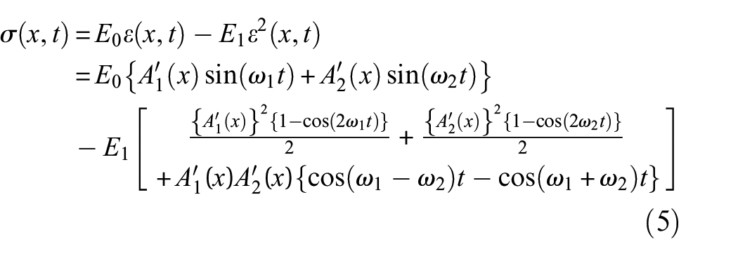
where
SPC-I technique
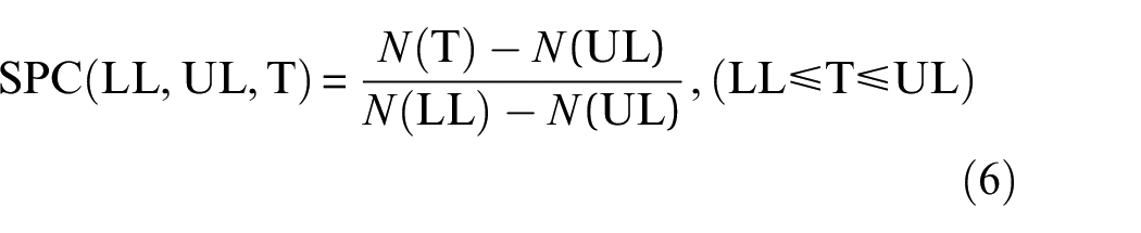
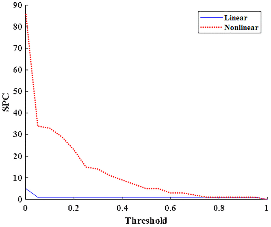
As mentioned in the previous section, when waves with certain frequencies propagate through a nonlinear material, new waves with frequencies other than the input waves are generated. 47 These new frequency peaks observed in the received signal spectrum can include higher harmonics, subharmonic, and other frequency peaks due to FM which are all called sideband peaks or simply sidebands. Sidebands are generally much smaller than the fundamental frequency peaks. The SPC technique, introduced by Eiras et al., 37 counts the sideband peaks above a moving threshold that moves between two limits—a lower limit and an upper limit (Figure 1). These SPCs are related to the nonlinearity of the material. The SPC curve in Figure 2 shows the variation in the number of counted peaks as the threshold value changes from the lower limit to the upper limit. The SPC expression can be given as follows:
where
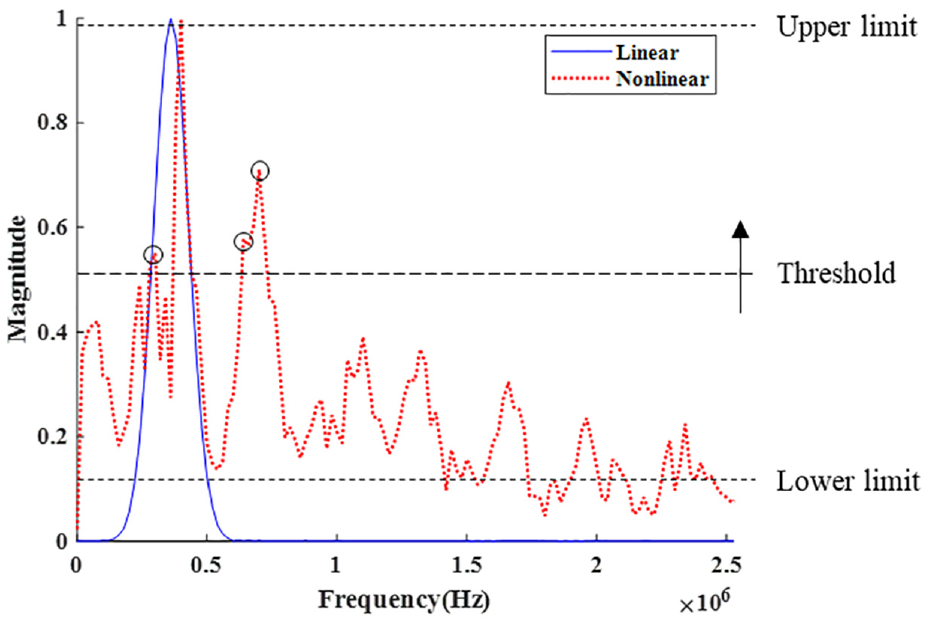
Illustration of the SPC technique—the curve with a single peak is generated by a linear material while the curve with multiple peaks is generated by a nonlinear material. As the threshold line moves upward, the number of counted sideband peaks decreases.
SPC curves generated by linear and nonlinear materials.
The SPC-I technique is an offshoot of the SPC technique, as introduced by Alnuaimi et al. 41 The SPC-I technique returns a single value by taking the average of the peak numbers in the SPC curve. SPC-I can be expressed as follows:
where
It has been verified by modeling and experiments that the SPC-I values increase as the number and size of micro-defects increase and decrease when micro-defects coalesce to form macro-defects.48,49 Therefore, it is important to note that not only the increasing trend of SPC-I be monitored but also its decreasing trend. In particular, the decrease in SPC-I after an increasing trend can indicate the formation of macro-defects and thus can represent the first signal of a structural failure.
Experimental program
Specimen
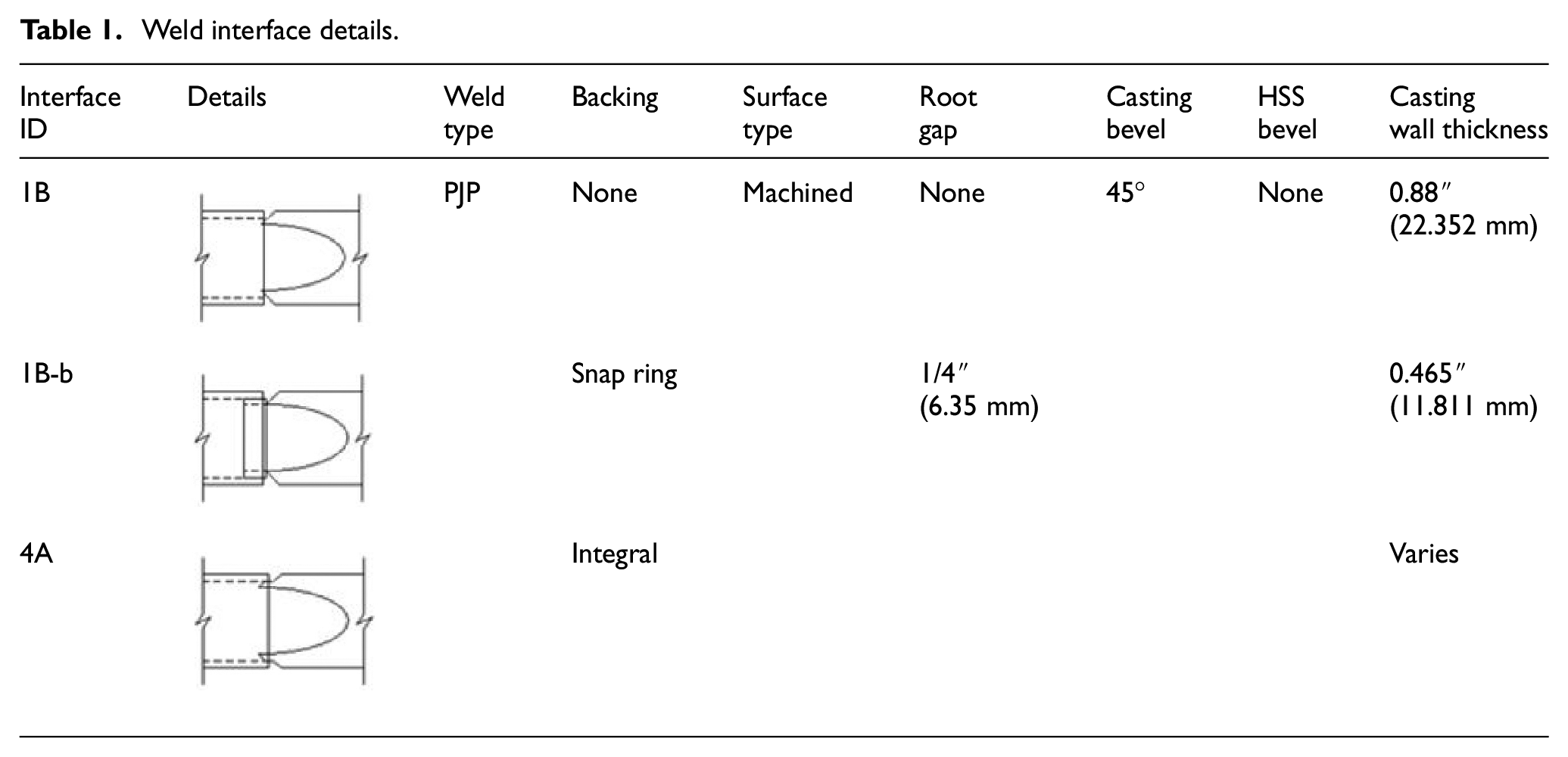
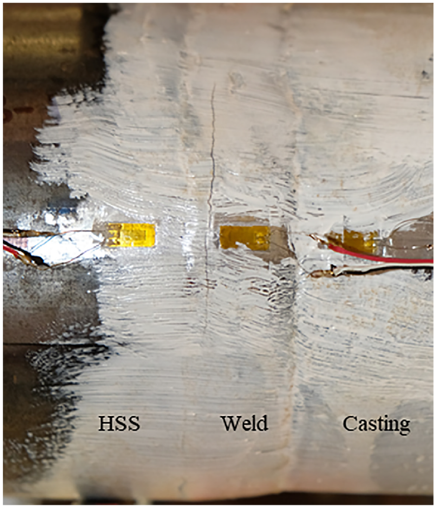
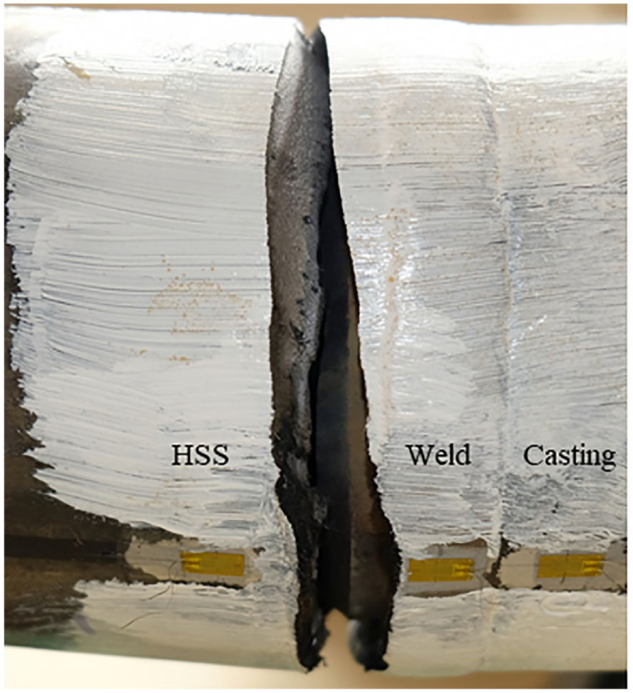
The specimens used in the experimental study are structural members composed of a central cast steel component welded to round hollow structural sections (HSS), that is, structural tubes, on either side (Figure 3). The cast steel is ASTM A958 Grade 8620 80/50 steel equivalent. The castings are provided by our industry partner and Steel Founders’ Society of America member Spokane Industries (Spokane Valley, WA, USA). Spokane performed a standard radiographic (RT) inspection of the cast components at the foundry. The RT confirmed the absence of any significant indications of damage in the casting at the welded interface region. The HSS members are American Society for Testing and Materials (ASTM) A500-18 Grade C steel. Fabrication of the welded specimens is performed by an American Institute of Steel Construction (AISC)-certified fabricator/erector JB Steel, Inc. (Tucson, AZ, USA). The weld types evaluated were partial joint penetration (PJP) groove welds, located between the casting and HSS.
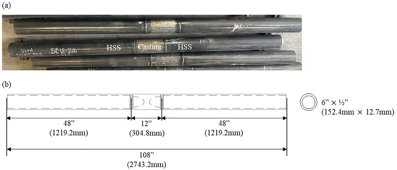
Welded test specimens: (a) photo and (b) dimensions.
Three welded interface configurations were evaluated in the experiments: (1) a PJP created using a 45 machined bevel in the casting; (2) the same detail also incorporating a backing ring; and (3) a detail incorporating a “built-in” backing ring cast integrally into the casting. Table 1 and associated schematics show each of these welded interface details and the pertinent information.
Weld interface details.
Instrumentation and data collection
The welded specimens were subjected to high-cycle fatigue loading conditions in a four-point bending test configuration. The load points flanked the cast component, placing both welded joints in the constant moment region (Figure 4). The specimens were cyclically loaded in a displacement-controlled fashion to produce a maximum and minimum stress of approximately 40 and 10 ksi (275.8 and 68.95 MPa), translating to a target stress range of 30 ksi (206.85 MPa) and a nominal stress ratio of R = 0.25. A loading rate of 3 Hz was selected, representing the maximum frequency of the dual servo-valve 55-kip (244.652 kN) actuator used in the testing that provided stable and repeatable loading amplitudes.
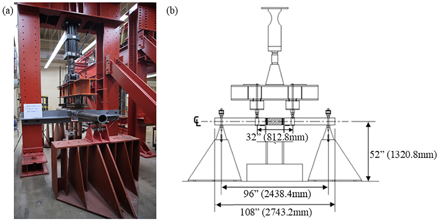
Four-point bending test setup: (a) photo and (b) schematic.
The instrumentation included two distinct sets of strain gages. One set consisted of two pairs of elastic strain gages placed at the extreme top and bottom lines or bending fibers of the cross-section and located midway between the end support and load application point on each HSS (Figure 5). This region is anticipated to remain elastic throughout the testing, and thus these gages are used to determine the internal flexural forces in the specimen for verification of the applied load, and quantification of any asymmetry in the setup. For this, classical Bernoulli beam theory is used to calculate the section curvature from the strain gage readings, and the resulting bending moment is calculated using principles of elasticity. The left- and the right-hand reaction forces are then approximated by assuming a point of inflection at the end supports. The nominal stress range for each test was determined by applying classical beam theory.
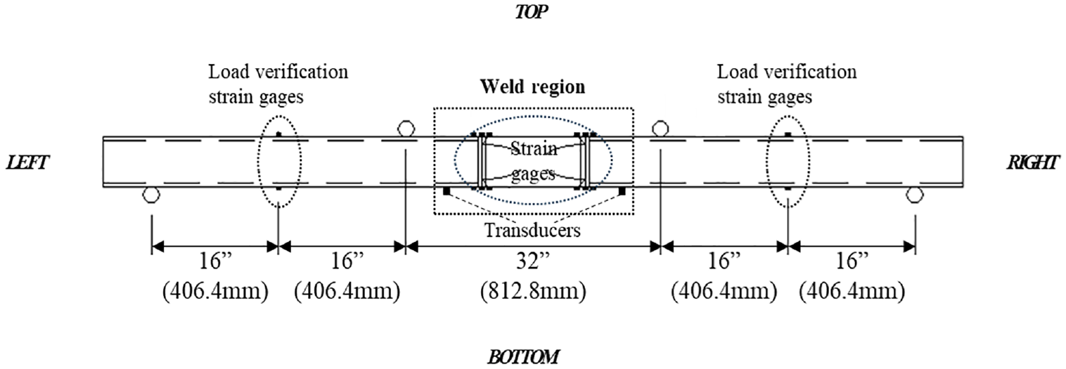
Placement of ultrasonic transducers and load verification strain gages.
The second set of strain gages was inelastic strain gages placed along the welded joint region between the HSS and casting (Figure 6). Each joint had three strain gages placed at its bottom most and topmost surface points: one was placed near the HAZ of the casting, one on the weld, and one near the HAZ of the HSS. Strain gages placed along the welded joint were positioned half an inch from the face of the weld on both the HSS and casting and one centered inside the width of the welded filler metal. The measured stress range for each location was calculated by measuring the local strain range from the gages and multiplying the measured modulus of elasticity from tensile coupons of the corresponding material. Note that for positive bending, the bottom extreme fiber would be in the critical tension region.
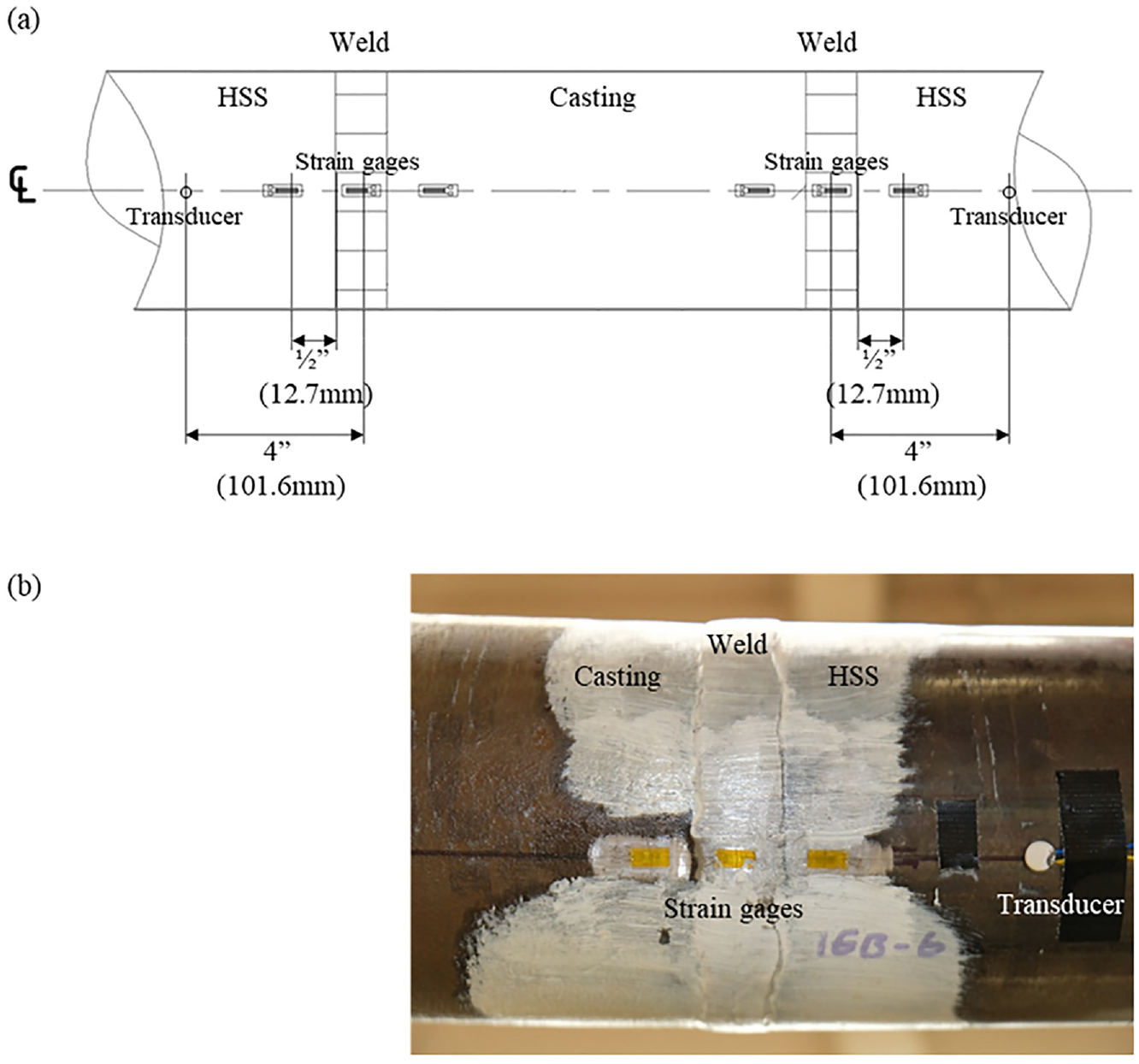
Placement of strain gages and ultrasonic transducers at the bottom of the weld region: (a) layout and (b) photo of the right side.
The fatigue tests were performed under the displacement-control condition. The displacement range associated with the stress range was first estimated using classical theory. Then each specimen was loaded monotonically under force control conditions to a proportion of the intended loading in the elastic range to confirm the target displacement while also monitoring the local strains (and corresponding calculated stress) of the weld region strain gages. For all tests, in the weld tension region, the HSS strain gages exhibited a higher strain than those on the weld and casting. Furthermore, one welded interface tended to have slightly higher readings due to inherent eccentricity in the system. This maximum reading is identified as the critical strain reading. Once a displacement and stress range were selected for each test, no alterations to the protocol (frequency or displacement amplitude) were made until the test was completed. Tests were terminated when a visible fracture was observed in the weld region which is denoted as the failure of the structure. Since a positive moment was applied, this region occurred at or near the extreme bottom fiber of the cross-section. Whitewash was applied to the welded regions on each specimen to see the cracks more clearly.
For ultrasonic NDT&E inspection, two ultrasonic transducers were used—one for excitation and the second one for receiving signals—in a transmission mode setup. Ultrasonic transducers were attached to the HSS flanking the two welded regions and placed 4 inches from the center of each welded joint (Figure 6). An ultrasonic signal with a central frequency of 230 kHz was excited and propagated through the welded joints. The nonlinear ultrasonic parameter SPC-I values were calculated from the received signal that was collected every 2 min (360 loading cycles). The schematic diagram of the ultrasonic NDT&E setup is shown in Figure 7.
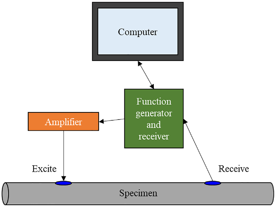
Schematic diagram of the ultrasonic NDT&E setup.
Experimental results
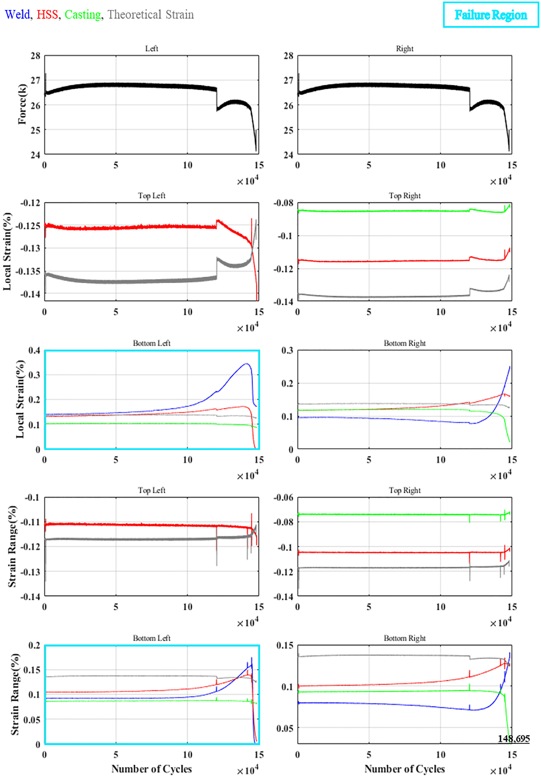
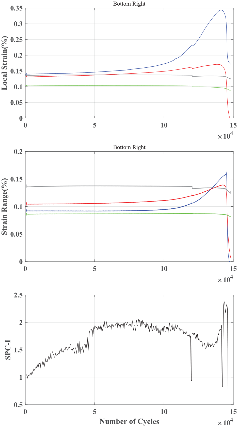
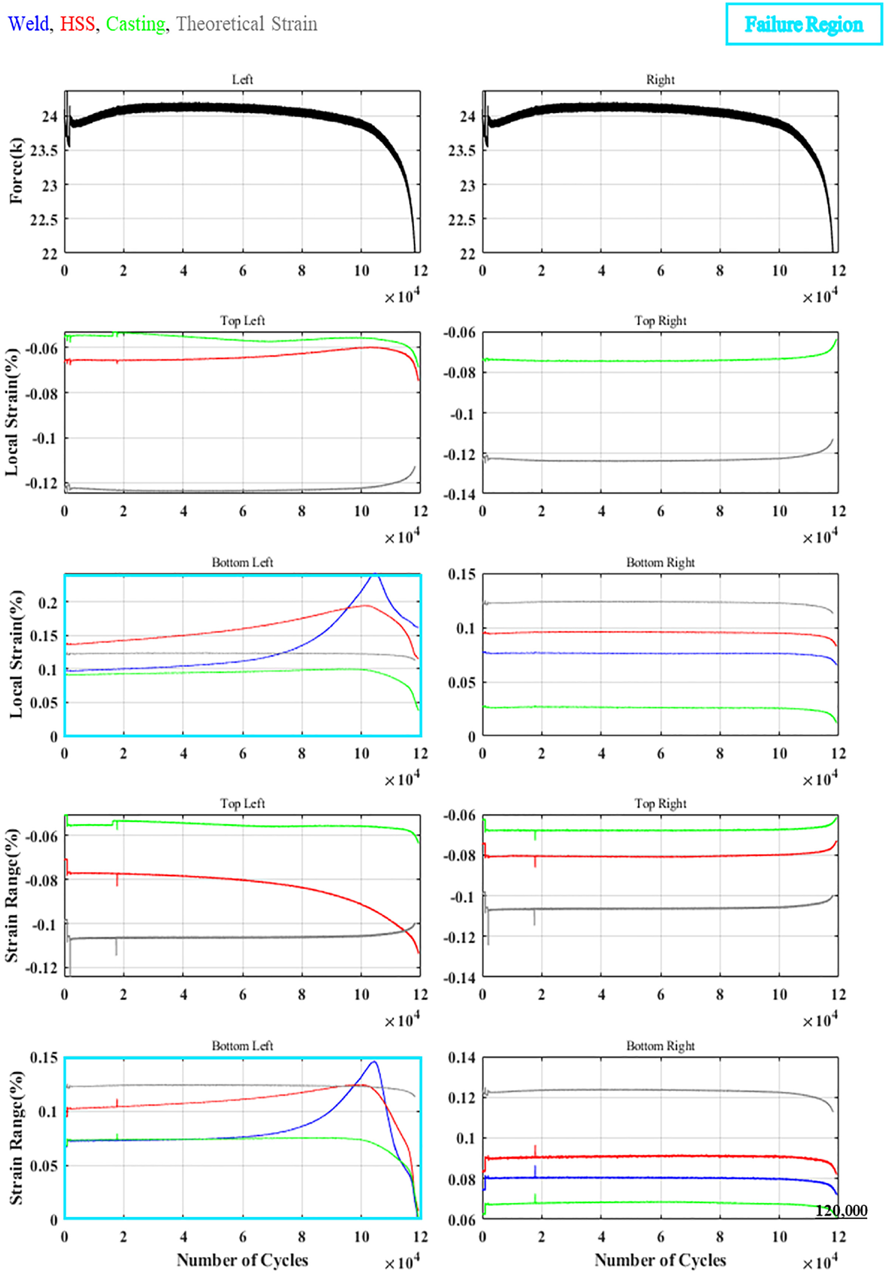
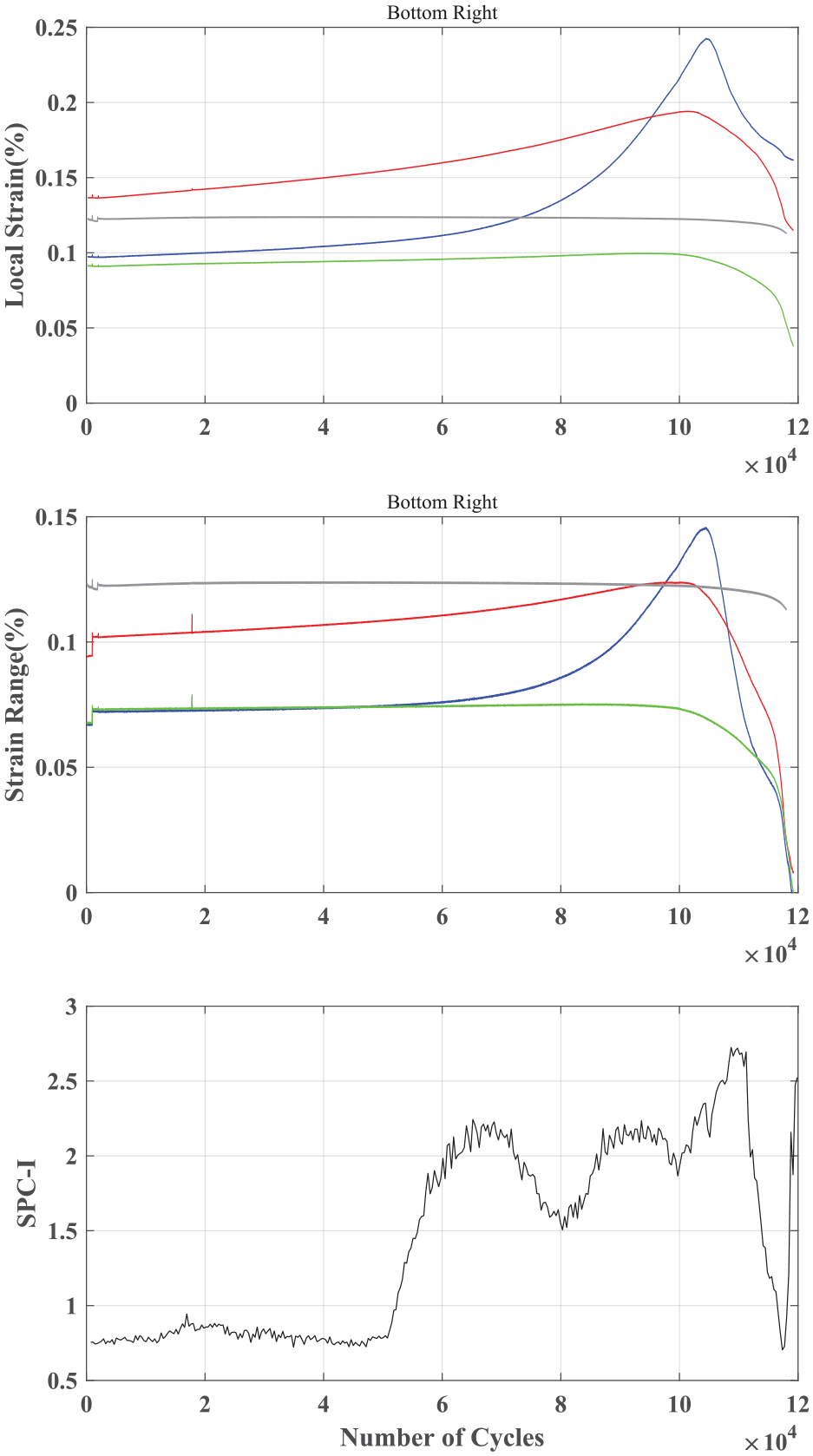
The results for each specimen are presented in the following order from top to bottom: (1) Applied force versus number of cycles; (2) local strain versus number of cycles; (3) strain range versus number of cycles; and finally (4) SPC-I versus number of cycles. The peak (maxima) global reaction force values at the left and right ends of the specimen for each corresponding cycle are included. Local strain is the peak (maxima) strain value for each cycle. The strain range is determined by subtracting the minima of each cycle from the maxima of the corresponding cycle. A theoretical strain calculation is added for each strain plot based on the global force (maxima of each cycle) for reference. In each plot, the weld strain values are indicated in blue, HSS strain values in red, and casting strain values in green. The local strain and strain range curves at the failure region for each test have also been indicated in a light blue box. The SPC-I plot is shown after the failure region local strain and strain range curves to clearly show how many cycles of loading SPC-I give a warning sign for the structural behavior. If the SPC-I value starts to decrease after reaching a local peak value, then it is considered an early warning predictor. This is because microcracks are first formed resulting in an increase in SPC-I values then they coalesce to form macrocracks, which reduces SPC-I value producing a hump in the SPC-I plot. The general trend of SPC-I variation ignoring the localized fluctuations is of our interest. Lastly, the close-up photos of the fractured region are shown.
Specimen 1B
Test results from strain gages for specimen 1B are shown in Figure 8. Note that for the applied positive moment, the top gages are always in compression (negative strain reading), while the bottom gages are always in tension. It can be observed that throughout the test, except at or near failure, the majority of the local strain readings exhibit stable behavior, with constant maxima within their material’s elastic limit (e.g., top left, top right, and bottom left regions). By contrast, the bottom right HSS and weld strain gages show an increase that continues until the end of the test where a noticeable fracture in the weld occurred. It is noted that the bottom right weld region had the highest initial strain and strain range among the four regions. Note that no weld strain gages were attached to this test specimen in the top (compression) region of the specimen.
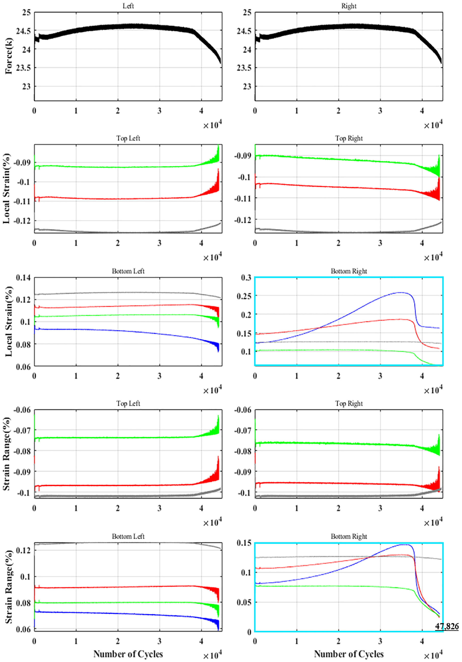
Strain gage data for 1B.
Figure 9 shows the corresponding SPC-I curve for specimen 1B, aligned by cycle number with the strain responses for the critical (bottom right) region. During the loading, the SPC-I value exhibits a steadily increasing trend until approximately 30,000 loading cycles. At this point, the SPC-I value starts to decrease. Thus, a hump is formed in the SPC-I plot. The hump indicates multiple microcracks are coalescing to form macrocracks. A reduction in the number of microcracks to form macrocracks lowers the SPC-I values resulting in the formation of the hump. Therefore, the reversal of the SPC-I trend (at ∼30,000 cycles) can be considered an early warning predictor for the impending structural failure. Note that the strain value reached a maximum value at around 35,000 before starting to go down as the loading was gradually reduced and finally stopped after 47,826 cycles when a visible crack appeared. At the end of the 47,826 loading cycles, the cracks developed in the pipe were closely inspected. Thus, all three parameters—strain, strain range, and SPC-I—could detect the impending failure before the appearance of visible cracks. In this test, the SPC-I gave the warning sign a little earlier (at 30 K cycles) compared to that given by the strain measurement (at 35 K cycles).
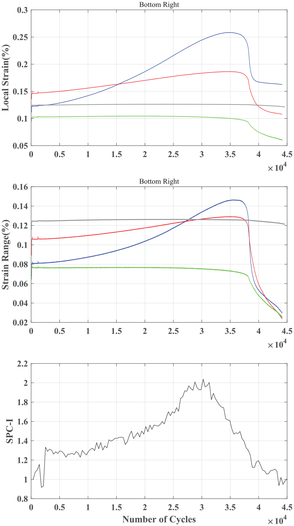
Local strain (top), strain range (middle), and SPC-I (bottom) variations with the number of loading cycles for specimen 1B.
Figure 10 shows a close-up photo of the failed weld where it can be seen that the fracture propagated along the weld and HSS interface. No other indication of failure or fracture developing was observed.
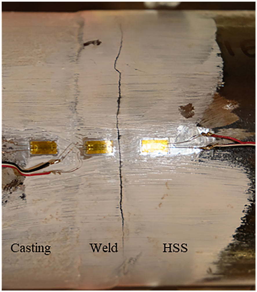
Specimen 1B weld fracture.
Specimen 1B-b
Test results from strain gages for specimen 1B-b are shown in Figure 11. It can be seen that both strain gages in the tension region of the weld exhibited an increase in strain when the test concluded. The bottom left weld strain began increasing approximately halfway through the test and continued until failure. The increased strain corresponds to a decrease in peak force as the fracture propagates. The marked drop in force at approximately 120,000 loading cycles is due to a pause in testing to check for visible fractures. Note that no strain gages have been applied to this test specimen at the top (compression) weld region of the specimen. In addition, the strain gage at the top left side of the casting is excluded due to a malfunction.
Strain gage data for 1B-b.
Figure 12 shows the SPC-I curve along with local strain and strain range curves for specimen 1B-b. The SPC-I value gradually increases until approximately 40,000 loading cycles then shows a sudden jump upward at approximately 50,000 loading cycles, indicating the likely formation of a large number of microcracks and or dislocations. After this sudden jump, the SPC-I value increases further until approximately 80,000 loading cycles, then it starts to decrease until approximately 100,000 loading cycles, indicating the likely coalescing of some of the microcracks to form macrocracks, which is an early warning predictor for potential failure. Another hump can be seen at around 110,000 loading cycles. The second hump implies the formation of more microcracks (as the SPC-I goes up) and coalescing of more microcracks to form macrocracks (as SPC-I again starts to go down). Therefore, two warning signs from the SPC-I measurement can be observed in this experiment before the structural failure (formation of the visible crack). Note that both the weld local strain and strain range values reached a maximum value at approximately 140,000 cycles before starting to go down as the loading was gradually reduced and finally stopped at 148,695 cycles. Interestingly, the weld strain range value starts to increase at approximately 50,000 loading cycles, coinciding with a sudden jump in the SPC-I plot, while conversely, the weld local strain shows a continuous increase.
Local strain (top), strain range (middle), and SPC-I (bottom) variations with the number of loading cycles for specimen 1B-b.
Figure 13 shows a close-up photo of the failed weld of specimen 1B-b. It can be seen that the fracture propagated along the interface between the weld and HSS. No other indication of fracture was observed along the circumference of the welds.
Specimen 1B-b weld fracture.
Specimen 4A
Test results from strain gages for specimen 4A are shown in Figure 14. The top right HSS strain gage is not shown due to an offset issue causing the reading to be excessively low. Note that the maximum strain readings remained relatively constant throughout the duration of this test, except for the bottom left strain gages. Both the bottom left HSS and weld strain readings started to increase until the test was terminated. A more significant increase occurs when the peak force begins to drop, and fracture develops along the outside surface of the weld.
Strain gage data for 4A.
Figure 15 shows the SPC-I curve along with maximum strain profiles for specimen 4A. A sharp increase in SPC-I values is observed between 50,000 and 65,000 loading cycles; followed by a decrease until 80,000 loading cycles, indicating the formation of a large number of microcracks during 50,000 to 65,000 loading cycles and then the formation of macrocracks due to coalescing of microcracks up to 80,000 loading cycles. This hump in the SPC-I plot can be regarded as the first warning sign of impending structural failure. The second hump is observed at approximately 95,000 loading cycles, which can be considered as the second warning sign. Thus, as before, two warning signs are provided by the SPC-I technique before the structural failure occurs when the visible cracks appear and the applied load is reduced. The third hump is observed after the structural failure. Note that both the local strain at the weld region and the stress range values became maximum at approximately 105,000 cycles, before starting to go down as the loading was gradually reduced and finally stopped at 120,000 cycles.
Local strain (top), strain range (middle), and SPC-I (bottom) variations with the number of loading cycles for specimen 4A.
Figure 16 shows a close-up photo of the fractured region of specimen 4A. The fracture developed along the weld and HSS interface can be seen in this photo. This test continued after the visible crack appeared allowing the crack to propagate along most of the weld circumference and the loading was terminated at approximately 120,000 loading cycles when the test data showed a significant drop in peak force.
Specimen 4A weld fracture.
Summary of observation
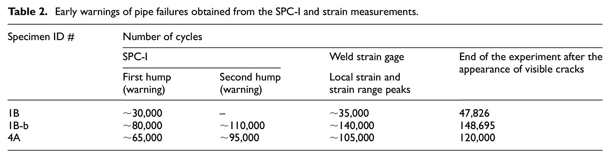
In this experimental investigation, the SPC-I curves showed a consistent trend giving one or more early warnings of impending structural failure for all three specimens considered here, as summarized in Table 2. Note that the local strain at the weld and strain range continuously increased until the resisting force at this displacement control test setup started to go down. Thus, strain gages cannot be used effectively as an early warning predictor for the impending structural failure of a component. The SPC-I technique, on the other hand, shows a clearly identifiable trend—a hump—that can serve as a warning sign. A hump is formed when the SPC-I values start to decrease followed by an increasing trend due to microcrack and macrocrack formations. This hump is observed well before the structural failure that becomes apparent from the appearance of visible cracks at the welded region. It should be emphasized here that the hump formation in the SPC-I plot indicates that the inspected structure has experienced increasing microcrack density (causing increasing trend of the SPC-I curve) followed by the macrocrack formation from the coalescing of microcracks and hence reduction in the microcrack density (causing decreasing trend of the SPC-I curve). Macrocrack formation does not necessarily automatically imply failure of the structure. Only when the generated macrocrack size exceeds the critical crack length for that structure, then it fails. Therefore, the SPC-I hump should only be interpreted as an indicator of the formation of macrocracks in the structure or an early warning before the actual failure. The sharpness of these humps can be related to the type of failure modes as discussed in the following paragraph.
Early warnings of pipe failures obtained from the SPC-I and strain measurements.
Due to the differences in the details of each casting weld interface, different types of crack formation were observed. Different mechanisms for crack initiation and propagation for the three specimens influenced the steepness or the gradient of the SPC-I curve differently. Comparing the post-test close-up photos for the three experiments (Figures 10, 13, and 16), it was concluded that the levels of fracture (or crack sizes) increased in the order: 1B-b, 1B, and 4A. This order can be related to the observed slope of the SPC-I variations (see Figures 9, 12, and 15). One can see that the SPC-I curve with a sharper hump is associated with a more severe fracture which produces a larger crack (Figures 9 and 15). The SPC-I curves with a lower hump (Figure 12) produce smaller cracks. Although there are differences in the steepness or the slope of the SPC-I curve, in all three cases, the early warning sign, which is a hump, is observed well before the structural failure. Recording both the SPC-I variation and the strain variation may be the best option for monitoring the damage progression in welded regions since the overall structural behavior can be determined from the strain values while the damage initiation (formation of microcracks) and its progression (when microcracks coalesce to form macrocracks) can be monitored from the rise and fall of the SPC-I values forming a hump in the SPC-I plot.
Conclusion
The purpose of this study is to examine the efficacy of the SPC-I nonlinear ultrasonic NDT&E technique in providing an early warning for impending failure of welded joints. Three specimens composed of cast steel components welded to round HSS were examined. Four-point bending tests of the welded specimen were conducted under fatigue loading conditions. Strain gages and ultrasonic transducers were attached to the specimens at the weld region to record strains and ultrasonic signals, respectively, in real time. For all experiments, strain data showed a continuously increasing trend until the failure. The failure was defined as when a sudden drop of the recorded stress values was observed and cracks in the welded region became visible. Clear warning signs—formation of humps—were observed in the SPC-I plot well before the structural failure. The results of this experimental investigation show that the SPC-I technique is a promising tool that can be implemented to detect and monitor the health of steel welded joints in real time. The recommendation from this investigation is that welded pipes in the field should be inspected for possible crack formation near the weld when a hump in the SPC-I curve is observed. A hump in the SPC-I plot indicates several microcracks after coalescing formed one or more macrocracks. After the formation of the hump if no visible cracks are detected on the weld surface or inside the weld using established nondestructive testing techniques, then the pipe may be allowed to operate until the second hump in the SPC-I plot is observed. The use of the pipe beyond a second hump is too risky and is not recommended. If the pipe failure can cause severe economic loss or loss of human life, then operating the pipe after the formation of the first hump is also not recommended. The SPC-I monitoring system can be used either as a continuous monitoring unit or for intermittent use where the data are collected at regular or irregular intervals. This monitoring technique can be used in either mode and should be decided by the user depending on the application and the criticality of the structure.
Footnotes
Acknowledgements
The mechanical testing portion of this research is sponsored by the DLA—Troop Support, Philadelphia, PA and the Defense Logistics Agency Information Operations, J68, Research & Development, Ft. Belvoir, VA, through the Steel Founders Society of America (SFSA) Digital Innovative Design (DID) Program. This support is greatly appreciated.
Declaration of conflicting interests
The author(s) declared no potential conflicts of interest with respect to the research, authorship, and/or publication of this article.
Funding
The author(s) received no financial support for the research, authorship, and/or publication of this article.
Disclaimer
The publication of this material does not constitute approval by the government of the findings or conclusion herein. Wide distribution or announcement of this material shall not be made without specific approval by the sponsoring government activity.