
Abstract
Existing intelligent fault diagnosis approaches demand substantial data for training diagnostic models. However, factors such as the inherent characteristics of bearings, operating conditions, and privacy security make collecting comprehensive fault-bearing data very difficult. Although generating synthetic data through generative adversarial networks (GANs) is feasible, the data generation of GANs is a time-consuming process. To address these challenges, a fault diagnosis framework based on GAN and deep transfer learning (DTL) is proposed, termed the simplified fast GAN triple-type data transfer learning (SFGAN-TDTL) method. Initially, an SFGAN is proposed as a replacement for traditional GANs. The time-frequency image data generated by SFGAN serve to augment the training dataset, offering faster and higher-quality data generation compared to traditional GANs. To further reduce time consumption for GAN-based methods, the TDTL method is proposed. Differing from DTL, which utilizes synthetic data to construct a pre-trained model and conducts targeted fine-tuning with real data, TDTL employs open-source data, synthetic data, and real data to fill the weights of the task-insensitive layer, task-sensitive layer, and fully connected layer, respectively. Numerical results demonstrate that SFGAN-TDTL maintains higher diagnostic accuracy while significantly reducing time consumption.
Keywords
Introduction
In the industrial landscape, the importance of bearings is paramount, serving as essential components that enable the seamless functioning of machinery, ensuring stability, reduced friction, and overall operational reliability.1,2 Bearings often operate under extreme conditions, experiencing severe vibrations, sudden temperature changes, and overweight loads. Consequently, they inevitably deteriorate over time, which can lead to machine failures, unplanned downtime, safety hazards, and significant economic losses.3,4 To this end, bearing fault diagnosis is crucial in equipment maintenance and upkeep.5–8
As big data continue to evolve, many fields resort to machine learning techniques to solve their problems.9,10 Widodo and Yang 11 employed support vector machines for fault diagnosis, Cerrada et al. 12 utilized random forests, and Sun et al. 13 used decision trees for the same purposes. As an extension of machine learning, deep learning is popular for minimizing human intervention by automatically extracting features. In fault diagnosis, deep learning networks have become increasingly popular. Shao et al. 14 proposed a hierarchical structure stacked with three restricted Boltzmann machines, thereby improving the classification accuracy. Qi et al. 15 proposed a novel fault diagnosis method using a stacked sparse autoencoder (SAE). The penalty term of the SAE is optimized to extract high-level fault features. However, deep learning networks are typically characterized by their data-intensive nature. This means that these networks often require substantial amounts of data for effective training and optimal performance. Specifically, large-scale datasets are essential to enable the network to learn and generalize patterns, features, and representations that can be applied to unseen or novel data, thereby enhancing the model’s overall capabilities and classification accuracy. In contrast to fields such as face recognition, defect inspection, and speech recognition, where data acquisition is relatively easy, gathering sufficient data from faulty bearings is exceedingly challenging for several reasons. First, the occurrence of bearing failure is often relatively infrequent. Second, bearing failure can manifest in various forms, increasing the complexity of data collection. Finally, it is crucial to note that data collection may involve proprietary or sensitive company information, subject to restrictions imposed by regulations and privacy policies.16,17 To overcome this challenge, data augmentation approaches such as simple transformation (e.g., adding noise) and digital twin have been widely used to generate sufficient fault data. Despite their usefulness, these methods have limitations. Simple transformation methods may not accurately capture the full diversity of faulty data, while digital twin methods may hard to simulate all fault features accurately. 18 Therefore, there is a need for a more effective data augmentation approach.
Generative adversarial network (GAN) was proposed by Goodfellow et al. 19 as an effective data augmentation approach. However, the original GANs are influenced by training instability and mode collapse due to various factors.20–22 Therefore, there are also numerous research results in the field of fault diagnosis. Zhou et al. 23 proposed a global GAN optimization mechanism to generate discriminant fault data and then filter out unqualified ones. Wan et al. 24 proposed a fast self-attentive deep convolution GAN (DCGAN), utilizing the self-attention module to focus on deeper data features and employing spectral normalization to enhance training stability. Fan et al. 25 proposed a GAN method that involves adding gradient normalization to the discriminator to enhance stability and incorporating a full attention module into the generator to extract deeper features. Although GAN-based fault diagnosis methods have demonstrated great potential in various applications, the data synthesis process is very time-consuming, posing great challenges. Given that most fault diagnosis scenarios demand high real-time capabilities, existing GANs may not be applicable. 26 Consequently, accelerating the training process of existing GANs to facilitate rapid data generation is a worthwhile research area, which has not been fully explored.
GAN-based fault diagnosis methods not only require time investment in data generation but also demand a considerable amount of time to train the diagnostic model on synthetic data.27,28 By leveraging pre-trained weights, deep transfer learning (DTL) can substantially reduce the required training data and accelerate the training process.29,30 Dong et al. 31 proposed a dynamic bearing physical model to generate simulation data. The knowledge acquired from the simulated data is then used in the training of diagnostic models. Zhong and Ban 32 proposed a transfer fault diagnosis method. The weights of shallow layers are obtained from a pre-trained CNN on the ImageNet database, whereas the weights of deep layers are customized to align with the target task. Li et al. 33 proposed a small sample wind turbine fault diagnosis method based on transfer learning and autoencoder, which acquire knowledge from similar wind turbines. Xu et al. 34 proposed a digital twin-assisted fault diagnosis method. This method employs DTL to transfer previously trained diagnostic models from the virtual space to the physical space.
To decrease the time consumption in fault diagnosis utilizing GANs, SFAGN-TDTL is introduced in this research. Our contributions are listed as follows:
(1) Combining the advantages of GAN and DTL, a fault diagnosis framework branded GAN-DTL is proposed. The time-frequency image data generated by the GAN are utilized to augment the training dataset, addressing the issue of insufficient data. The DTL leverages these synthetic data to build a pre-trained model for better performance.
(2) To reduce the training time of the diagnostic model based on GAN-DTL, a triple-type data transfer learning (TDTL) method is proposed. For the diagnostic model, the weights of the task-insensitive layer are trained on an open-source database, thus reducing training time through preloading. Subsequently, the weights of the task-sensitive layer are obtained from synthetic data, and the fully connected (FC) layer is fine-tuned with real data to align with the task target.
(3) To accelerate the data generation of GAN, SFGAN is proposed to synthesize data with improved image quality and faster speed. One key component of SFGAN is the lightweight skip connection (LSC) module, which utilizes skip connections to enhance gradient flow and incorporates 1 × 1 convolutions based on this approach.
(4) In light of both SFGAN and TDTL, a novel GAN-based fault diagnosis model called SFGAN-TDTL is proposed, integrating both methods to classify bearing faults. Experimental results demonstrate its superior performance, particularly in small sample scenarios, including higher diagnostic accuracy, rapid data generation, and quicker model training.
The rest of the paper is organized as follows. In the following sections, preliminaries are presented, the proposed SFGAN-TDTL method is detailed, and the comparison experiments on two representative bearing datasets are introduced. Finally, a conclusion is drawn in the final section.
Preliminaries
Deep transfer learning
convolutional neural network (CNN)-based DTL involves network models in both the source and target domains.
35
Among the pre-trained model

where

where

where
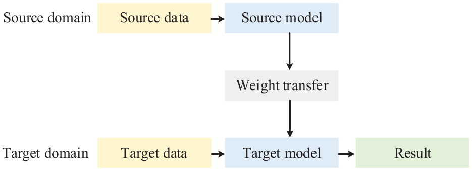
Typical architecture of DTL.
Generative adversarial network
The basic idea of GAN is to use generator
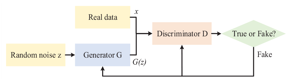
Typical architecture of regular GAN.
The optimization of GAN is equal to

where
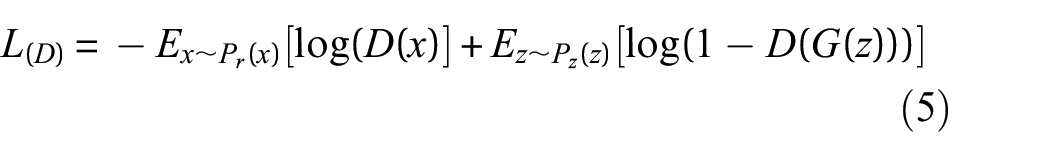
where
The proposed SFGAN-TDTL method
Overview of GAN-DTL
This section provides a systematic description of SFGAN-TDTL. First, a brief introduction to GAN-DTL is provided, which is shown in Figure 3. The real data are imported to GAN. Afterward, the source model undergoes learning using synthetic data, and its trained weights are transferred to the target model. Finally, the target model is fine-tuned with real data and gives diagnostic results.
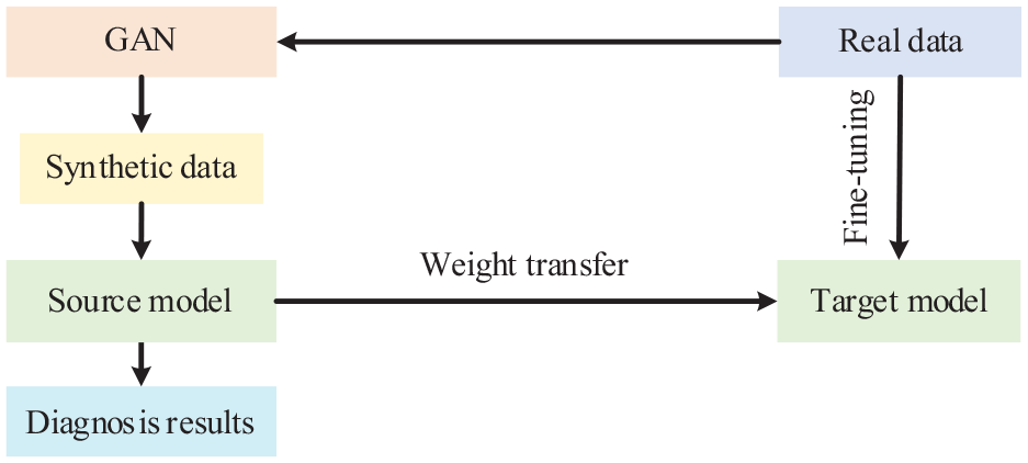
Basic flowchart of GAN-DTL.
Triple-type data transfer learning
Deep CNNs demonstrate broad applicability in intelligent fault diagnosis. However, their substantial size, comprising millions or even billions of learned parameters, makes them time-consuming to deploy in practical industry applications. 36 In response to this challenge, researchers have explored DTL, leveraging pre-trained models to reduce training time. Typically, models are pre-trained on open-source data and subsequently fine-tuned with real data, as shown in the upper left of Figure 4. Nevertheless, open-source data are not tailored for the target task, making it challenging to achieve satisfactory performance. Simultaneously, some studies utilize synthetic data generated by GANs to train models but encounter two time-related challenges. First, the generation time of synthetic data is notably lengthy. Second, unlike open-source data, the training of synthetic data cannot be preloaded, thereby extending time consumption. To address the above challenges, TDTL is proposed based on DTL and GAN, integrating three types of data to decrease time consumption while maintaining high performance.
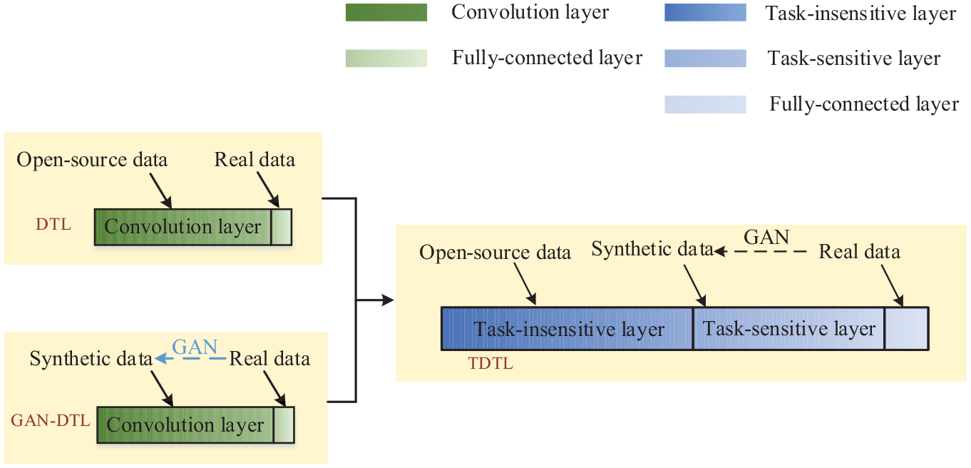
Diagram of DTL: GAN-DTL (green) and TDTL (blue).
In most CNNs, shallow layers learn common features, and deeper layers learn more specific features for a given task.
37
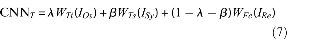
This phenomenon results in shallow weights having less impact on the result, while deep weights have a greater impact. Therefore, all the convolutional layers are artificially divided into task-insensitive and task-sensitive layers, as shown in the right half of Figure 4. The task-insensitive layer is defined as being insensitive to the target task, while the task-sensitive layer is defined as being sensitive to the target task. The task-sensitive layer undergoes learning using open-source data as the part of pre-trained model. Then, the task-sensitive layer is trained on synthetic data. Finally, the FC layer is fine-tuned with real data, the same as in DTL. Hence, the weight structure of the
where

Since TDTL involves three types of data, its specific operational steps include training the pre-trained model, the source model, and the target model, as shown in Figure 5. The detailed operational process is as follows:
(1) Pre-trained model: Pre-train and save the weights of task-insensitive layers.
(2) Source model: Inherit the weights of the task-insensitive layer from the pre-trained model and freeze it. Subsequently, train with synthetic data while saving the weights of task-sensitive layers.
(3) Target model: First, inherit the weights of the task-insensitive layer from the pre-trained model. Then, inherit the weights of the task-sensitive layer from the source model. Finally, fine-tune the FC layer with real data.
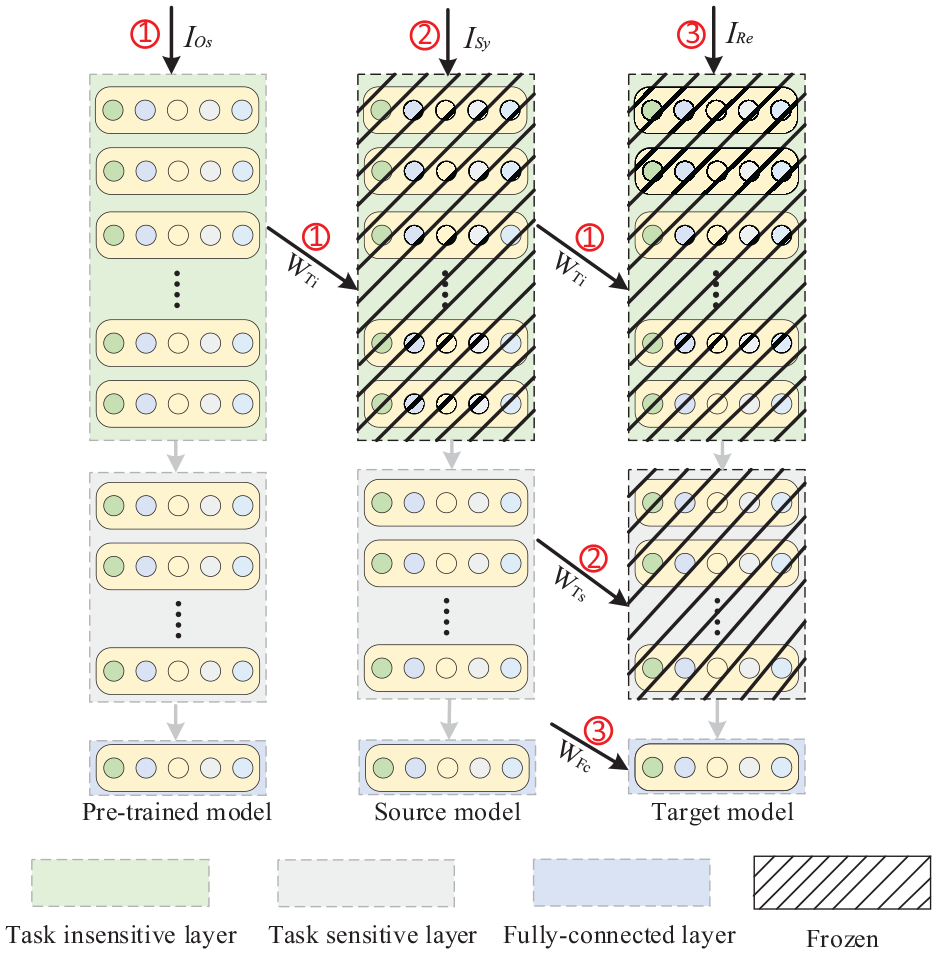
Detailed operational process of TDTL.
Simplified fast GAN
While GANs are extensively employed for data synthesis, the process is time-consuming due to the numerous parameter weights inherent in GANs. These weights contribute to a slowdown in the data synthesis process.
38
Targeting this challenge, SFGAN is proposed to speed data generation through the proposed LSC module. First, LSC contains two inputs, which are the low-resolution
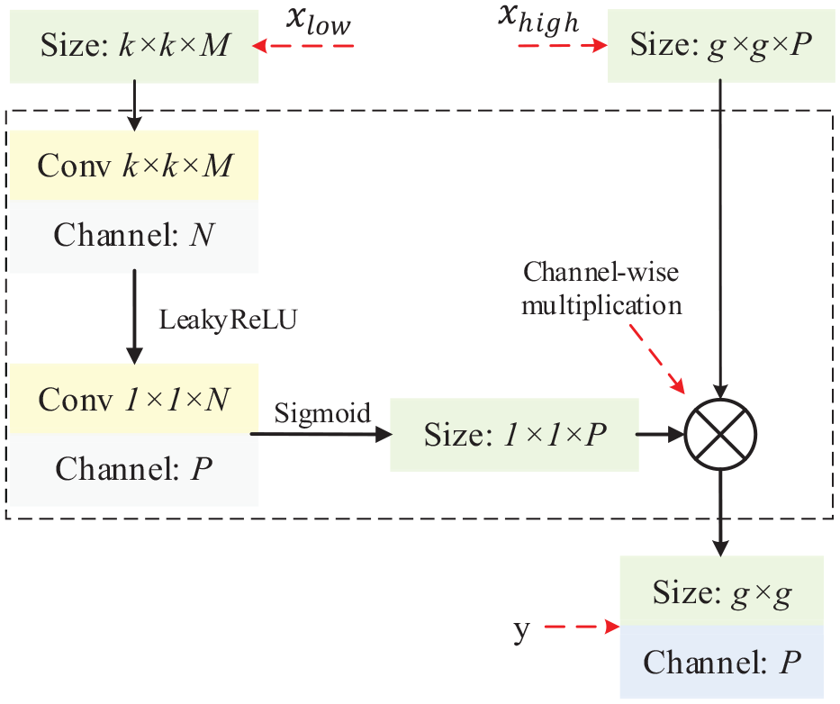
Architecture of the LSC module.
Skip connection
Smooth gradient flow in deep learning networks promotes faster convergence, stable training dynamics, and addresses issues such as vanishing and exploding gradients. It enhances generalization, simplifies hyperparameter tuning, and facilitates efficient parallelization in distributed computing environments. A robust gradient flow can be enhanced with skip connections.
39
Therefore, a skip connection is implemented between
1 × 1 convolution
The 1 × 1 convolution in deep learning networks is advantageous for its computational efficiency, capacity for dimensionality reduction, and ability to amplify expressiveness, leading to improved model efficiency and performance.
40
In the study, 1 × 1 convolution and channel multiplication are employed. Initially, the spatial dimension of

where
Finally, LSC is integrated into the generator, which is shown in Figure 7. More specifically, the two LSC modules are embedded between 4 × 4 resolution and 64 × 64 resolution, 8 × 8 resolution, and 128 × 128 resolution.
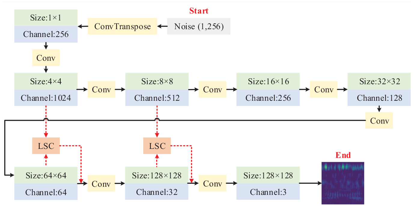
Structure of SFGAN.
Procedure of the proposed SFGAN-TDTL method
Most GAN-based fault diagnosis methods typically involve three key stages: data sample construction, data synthesis, and model training. Initially, time-frequency images are chosen for data sample construction due to two primary reasons. First, time-frequency images align better with the input format requirements of deep learning networks. Second, the time-frequency image effectively highlights diverse fault characteristics, offering clear discrimination. In the data synthesis stage, SFGAN is employed with real data to generate synthetic data. Subsequently, in the model training phase, TDTL is applied. Figure 8 depicts the basic flowchart of SFGAN-TDTL, expressed as follows:
(1) Different types of vibration signals are collected from rolling bearings. Subsequently, the fault signals are transformed into time-frequency images, that is, real data, through continuous wavelet transform (CWT).
(2) Train a complete SFGAN with real data, followed by the generation of synthetic data using the SFGAN generator.
(3) The insensitive layer is trained with open-source data, and its weights are transferred to the target model. Subsequently, the sensitive layer learns from synthetic data, and its weights are applied to the target model. Ultimately, the FC layer of the target model is adjusted using real data.
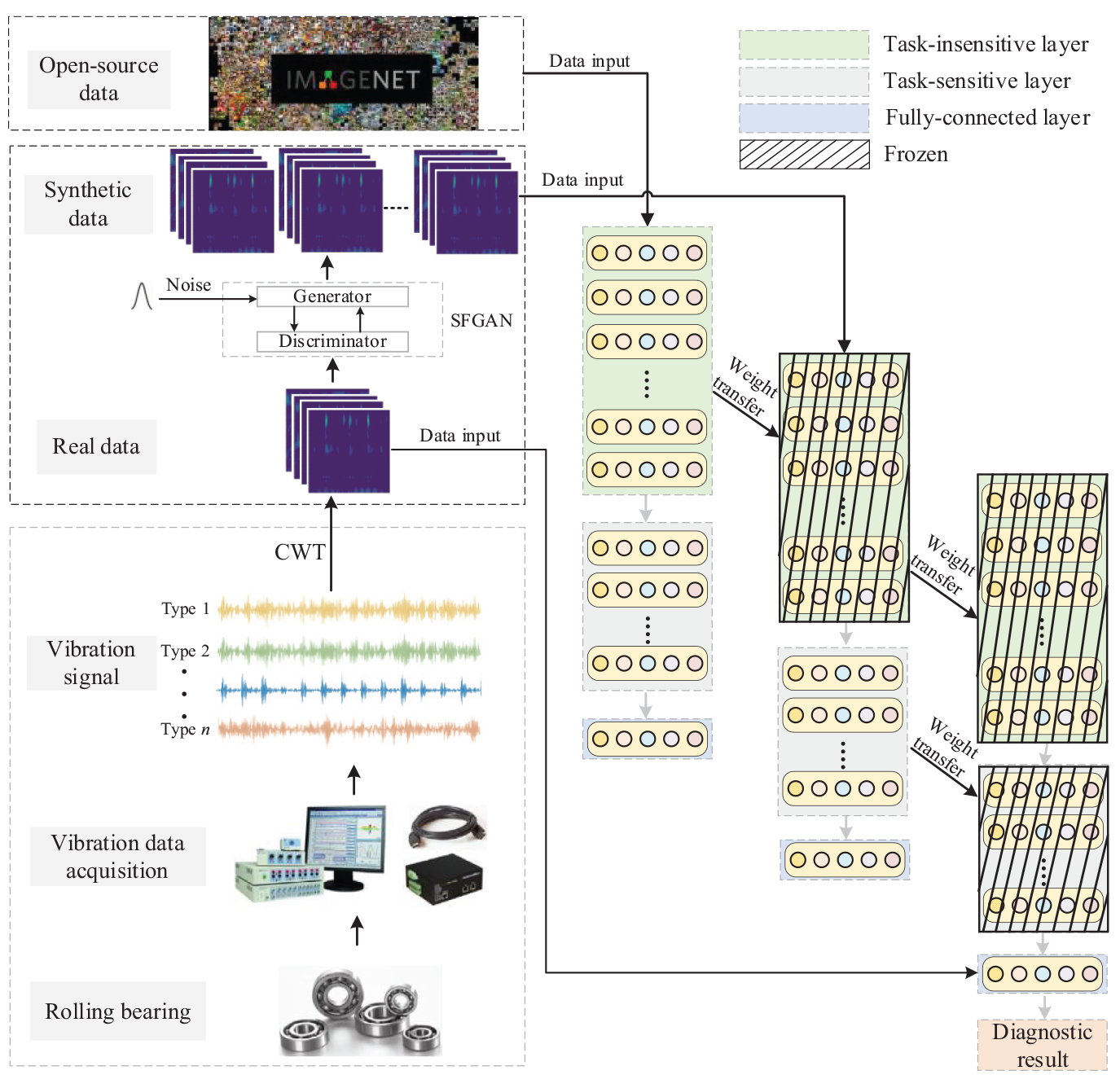
Architecture of the SFGAN-TDTL method.
Case study and experimental results
Case study 1: CWRU-bearing dataset
Dataset description
Currently, the most widely used dataset for bearing fault diagnosis is the Case Western Reserve University (CWRU) dataset. 41 The experimental setup includes a 2 HP induction motor, a torque sensor/encoder, and a dynamometer, as shown in Figure 9. In addition, the control electronics, although not visible, are also part of the setup. The driving end of the induction motor is equipped with test bearings, and the sampling frequency is set at 12 kHz.
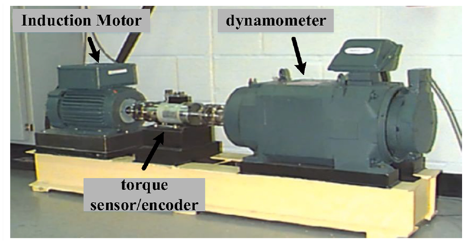
CWRU experiment equipment.
Different bearing health conditions are considered, including ball fault, inner-race fault, and outer-race fault. These faults are made by an electro-discharge machine, and all the diameters are 0.007 inch. The details of the dataset are listed in Table 1.
Details of the CWRU dataset.
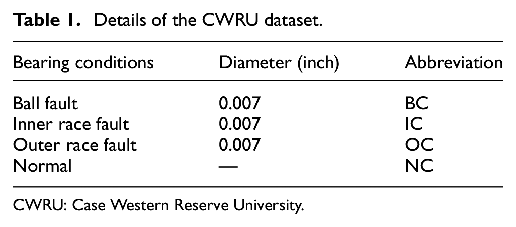
CWRU: Case Western Reserve University.
As described in Section “Procedure of the proposed SFGAN-TDTL method,” CWT is employed to transform raw vibration signals into time-frequency images. For time-frequency conversion, the four types of signal segments in the CWRU dataset are uniformly set to 1470. 42 Then, the raw vibration signals are converted into time-frequency images, which are shown in Figure 10.
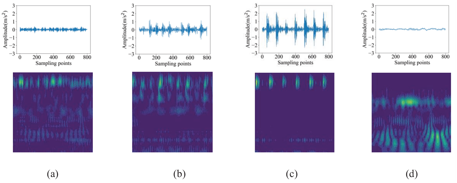
Time-frequency images of four states on the CWRU dataset: (a) BC, (b) IC, (c) OC, and (d) NC.
Effectiveness of TDTL
TDTL is proposed as a transfer learning methodology that leverages open-source data, synthetic data, and real data. The primary objective is to reduce training time while maintaining high diagnostic accuracy, especially in small sample scenarios. Therefore, to systematically evaluate the effectiveness of TDTL, conduct comprehensive comparisons encompassing diverse training methods and varying synthetic data quantities. Considering that TDTL inherently utilizes GAN, for a more precise description, it can equivalently be referred to as GAN-TDTL. First, the three comparison training methods are outlined: (a) DTL: this approach leverages open-source data to train CNN and fine-tune it; (b) GAN-CNN: this approach uses synthetic data to train CNN; and (c) GAN-DTL: this approach uses synthetic data to train CNN and fine-tune it with real data. To enhance clarity in illustrating the above training methods, diagrams for each method are shown in Figure 11.
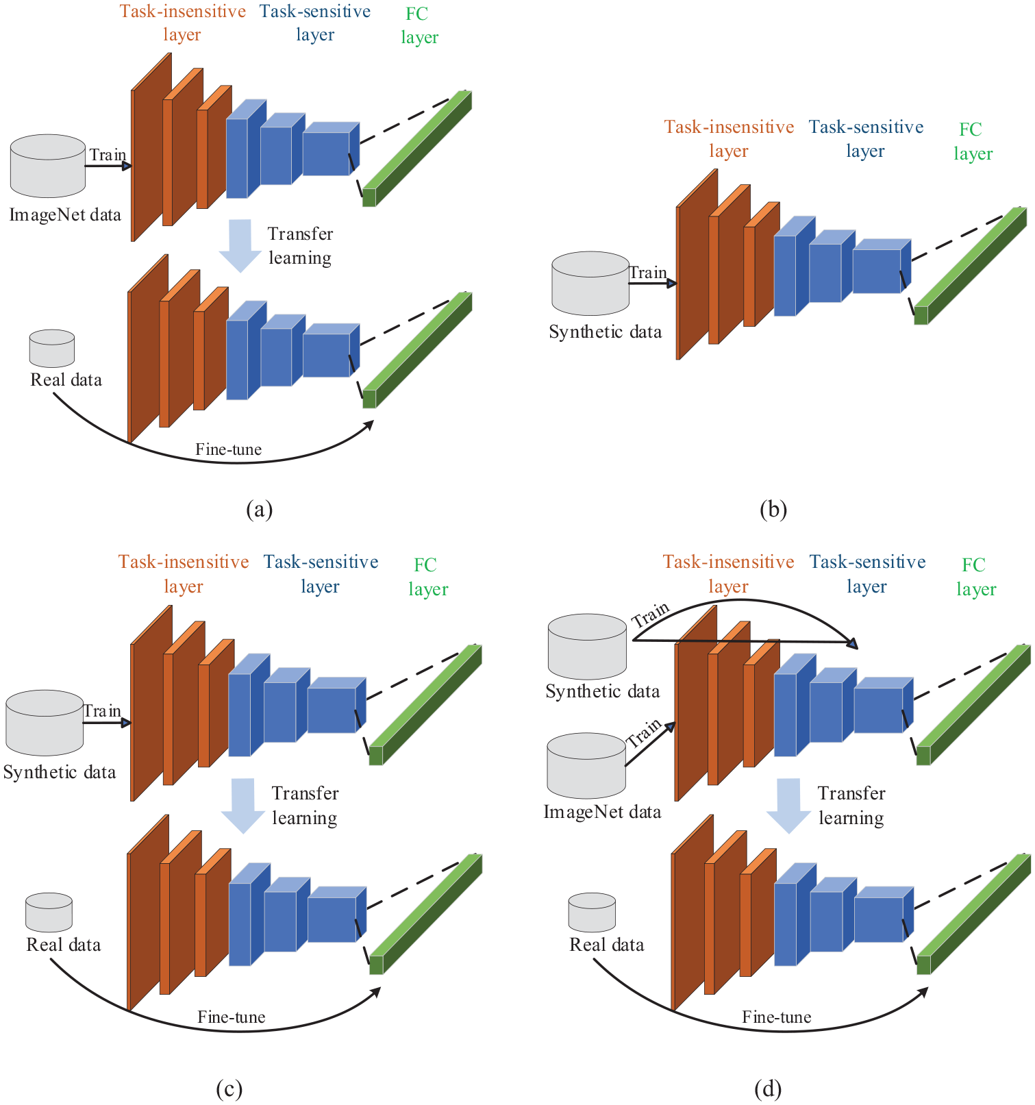
Diagrams of (a) DTL, (b) GAN-CNN, (c) GAN-DTL, and (d) GAN-TDTL.
In the comparative experiments, a standardized CNN model is employed, and the synthetic data are uniformly generated with DCGAN. 43 The ImageNet dataset is set as open-source data, and its quantity is sufficient. 44 To establish a control group, three distinct sets of synthetic data, comprising 2000, 4000, and 6000 samples, are created. The quantitative results encompass two key metrics: time consumption (min) and accuracy (acc). The models are run on the Pytorch framework with Intel(R) Core R7-5800H CPU (16GB RAM), and RTX3060 GPU. Detailed numerical results are comprehensively presented in Table 2.
Comparison results of time consumption and accuracy.
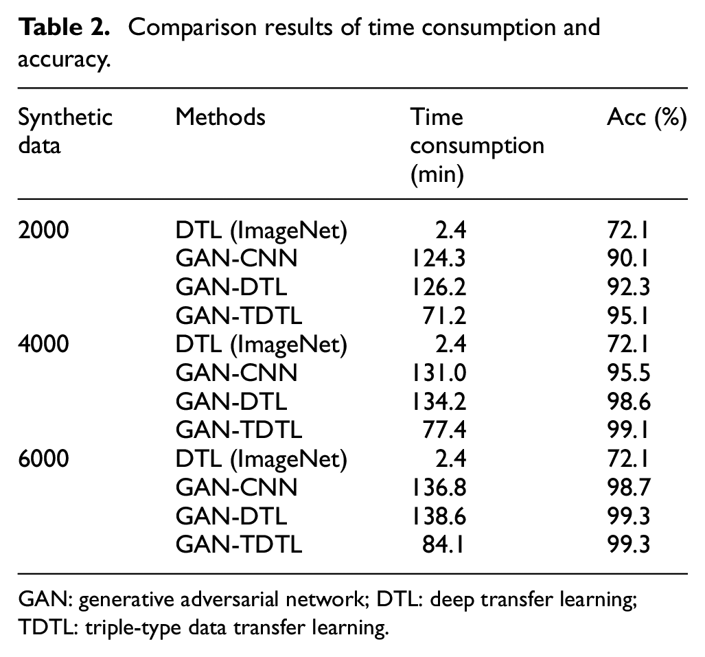
GAN: generative adversarial network; DTL: deep transfer learning; TDTL: triple-type data transfer learning.
Table 2 shows that GAN-TDTL achieves the highest accuracy under the three sets of synthetic data. For instance, with 2000 synthetic data, GAN-TDTL achieves 95.1% accuracy, which is 2.8% and 5.0% higher than the GAN-DTL and GAN-CNN, respectively. With 4000 synthetic data, the accuracy of GAN-TDTL increases to 99.1%, which is 0.5% and 3.6% higher than GAN-DTL and GAN-CNN, respectively. However, as the amount of synthetic data increases, the accuracy increase of GAN-TDTL becomes less significant compared to GAN-DTL and GAN-CNN. With 6000 synthetic data, GAN-TDTL has the same accuracy as GAN-DTL and is only 0.6% higher than the GAN-CNN. From the above analysis, it is evident that GAN-TDTL achieves the highest accuracy by leveraging ImageNet data to compensate for the insufficiency of synthetic data (2000, 4000). However, when synthetic data are abundant (6000), the advantage of ImageNet data participation in TDTL diminishes. Given that this study primarily concerns small sample scenarios, it can be concluded that the accuracy of GAN-TDTL surpasses that of other methods being compared. Furthermore, with 2000, 4000, and 6000 synthetic data, the model training time of GAN-TDTL is reduced by 55.0, 56.8, and 54.5 min compared to GAN-DTL and GAN-CNN. In summary, GAN-TDTL exhibits higher accuracy and shorter training time in small sample scenarios.
Effectiveness of SFGAN
To verify the effectiveness of SFGAN, real data are imported into DCGAN, WGAN, 45 CGAN, 46 and SFGAN, to generate synthetic data. Following that, two indices, structural similarity (SSIM) and Fréchet inception distance (FID), are employed for a quantitative analysis of the images. SSIM is defined as:
where
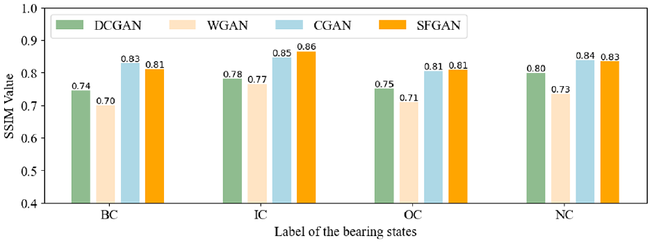
Comparison of GANs on SSIM.
In Figure 12, the average SSIM values of DCGAN, WGAN, and CGAN are 0.767, 0.727, and 0.832, respectively. The average SSIM value of SFGAN is only lower than that of CGAN, with an average of 0.825. Next, FID is defined as:
where
Comparison of GANs on FID.
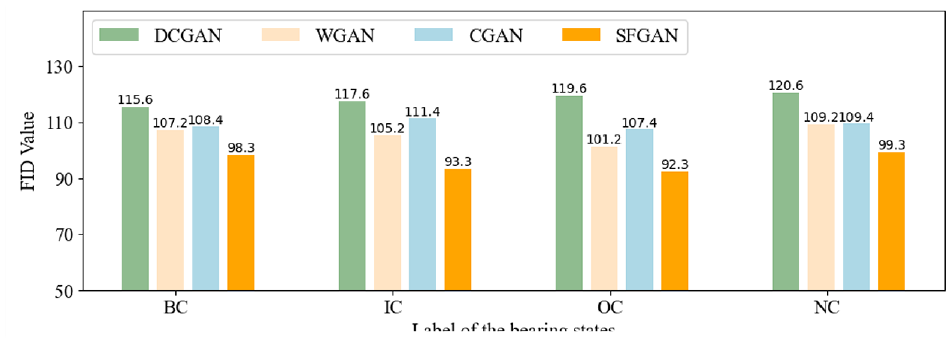
In Figure 13, the average FID values of DCGAN, WGAN, and CGAN are 118.35, 105.7, and 109.9, respectively. SFGAN gives a lower average SSIM than these three GANs with an accuracy of 95.82. Overall, both the SSIM and FID values offered by SFGAN consistently exceed those of other GANs, demonstrating that the synthetic data generated by SFGAN achieve high quality. Furthermore, the time and image quality of various GANs are added to the comparison, which is shown in Table 3.
Overall performance of the SFGAN and comparison GANs.
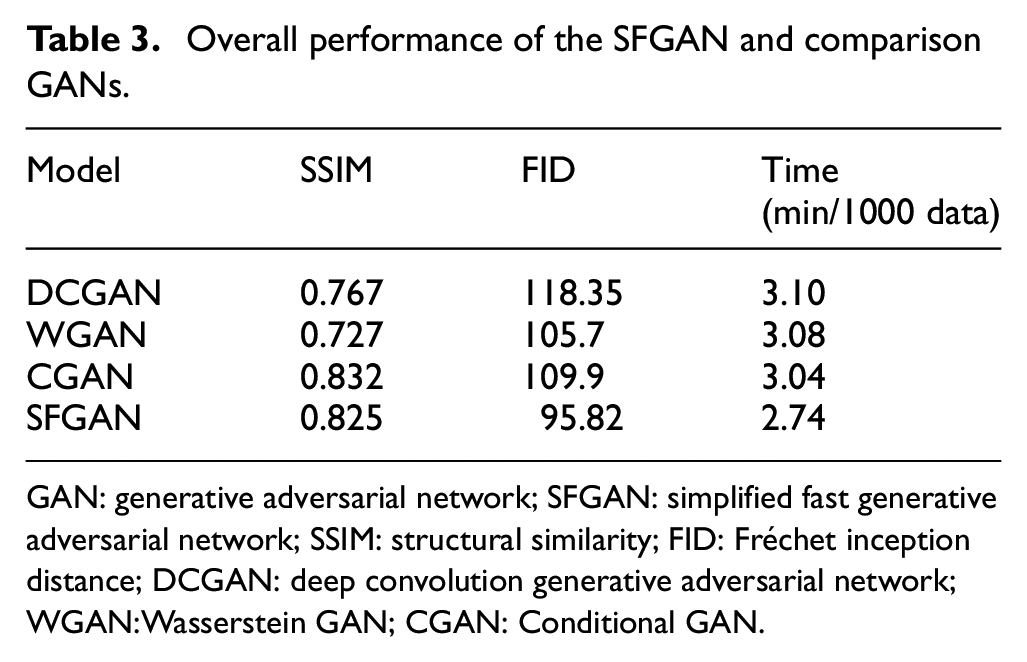
GAN: generative adversarial network; SFGAN: simplified fast generative adversarial network; SSIM: structural similarity; FID: Fréchet inception distance; DCGAN: deep convolution generative adversarial network; WGAN:Wasserstein GAN; CGAN: Conditional GAN.
From Table 3, SFGAN shows the shortest data generation time of 2.74 min/1000 data, which is 11.6% shorter than the second-ranked CGAN (3.04 min). In addition, the relationship between data generation time and image quality is shown in Figure 14, where the x-axis, y-axis, and z-axis represent SSIM value, FID value, and data generation time, respectively.
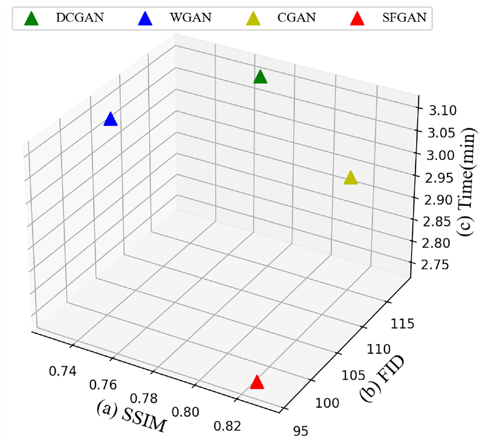
Comparison of different GANs on three indicators: (a) SSIM, (b) FID, and (c) data generation time.
As shown in Figure 14, SFGAN reaches the best balance between image quality and generation time. These results show that SFGAN minimizes the time needed to synthesize data without compromising image quality.
Comprehensive performance evaluation of SFGAN-TDTL
To thoroughly evaluate the effectiveness of SFGAN-TDTL, an ablation experiment is conducted, involving different transfer learning methods, including DTL and TDTL, as well as data augmentation methods such as GAN and SFGAN. The purpose is to determine which components of SFGAN-TDTL contribute most to its overall performance. The experimental results on 2000, 4000, and 6000 synthetic data are shown in Table 4.
The results of ablation studies.
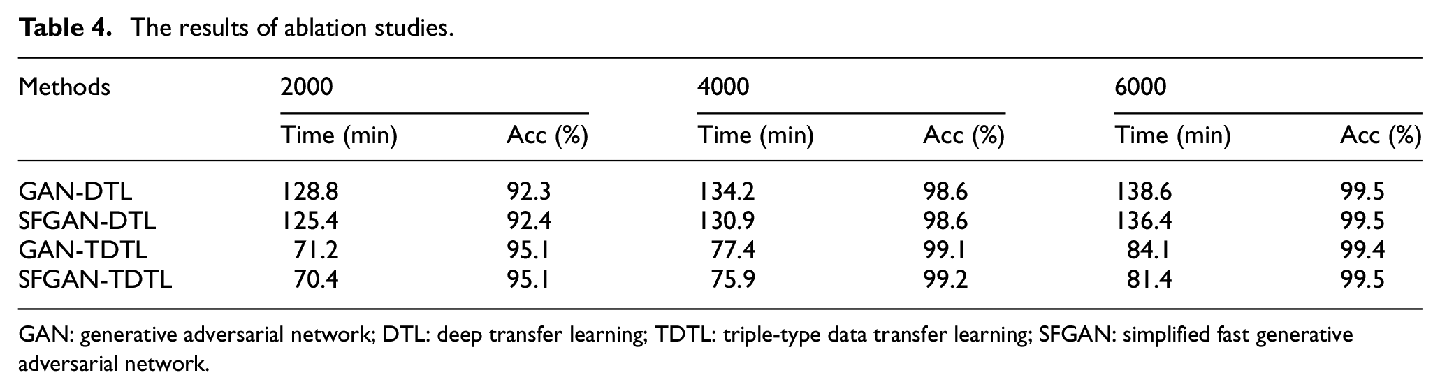
GAN: generative adversarial network; DTL: deep transfer learning; TDTL: triple-type data transfer learning; SFGAN: simplified fast generative adversarial network.
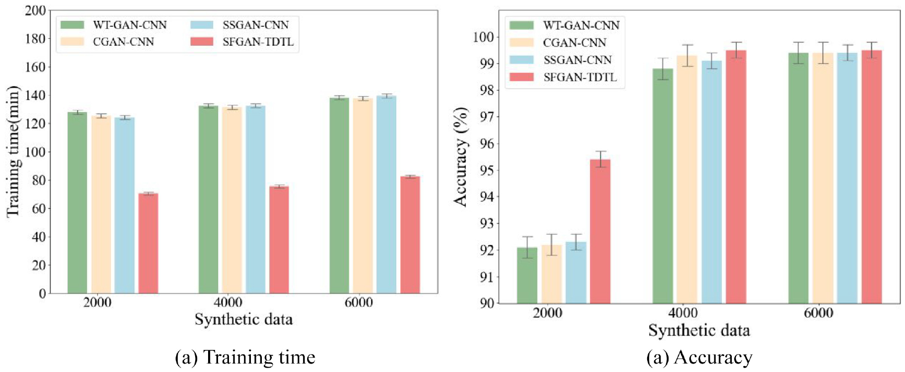
From Table 4, it is observed that using SFGAN instead of GAN reduces the data generation time by 13%. Besides, comparing SFGAN-DTL to SFGAN-TDTL, TDTL requires 47% shorter training time than DTL. In addition to these experiments, three state-of-the-art GAN-based fault diagnosis methods are supplemented to the experiment for comparison, as shown in Figure 15.
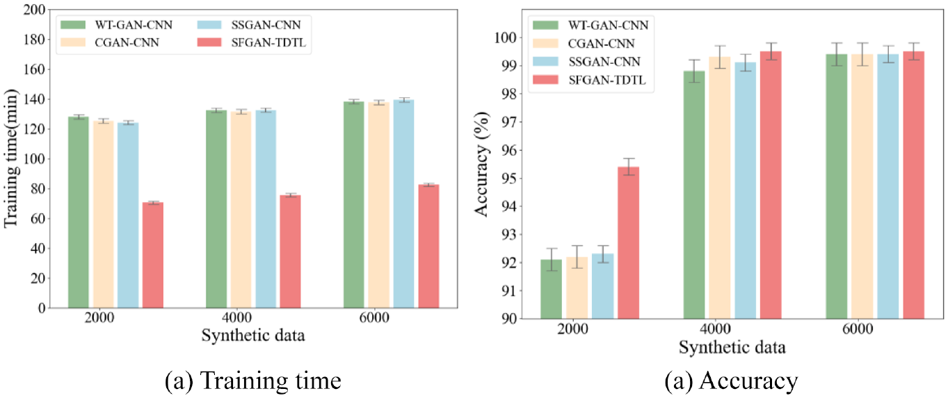
Performance comparison on the CWRU dataset: (a) Training time; (b) Accuracy.
In Figure 15(a), the time consumption of SFGAN-TDTL on the sets of 2000, 4000, and 6000 synthetic data is lower than that of its competitors. Specifically, the time of SFGAN-TDTL is 45, 47, and 48% less than WT-GAN-CNN, 47 CGAN-CNN 45 and SSGAN-CNN, 48 respectively. The significant advantages of SFGAN-TDTL become evident, emphasizing its efficiency in terms of time consumption. Notably, the 2000 synthetic dataset in Figure 15(b), SFGAN-TDTL achieves higher diagnostic accuracy, surpassing WT-GAN-CNN, CGAN-CNN, and SSGAN-CNN by 0.31, 0.32, and 0.28%, respectively. This demonstrates that with the assistance of a pre-trained model, SFGAN-TDTL can attain higher accuracy with a shorter time and less data.
Case study 2: SBTR-bearing dataset
Dataset description
The proposed method has been validated on the CWRU dataset. We further investigate the performance of this method on the SBTR dataset, and its test rig is shown in Figure 16. This extension aims to evaluate the generality and robustness of the proposed method across different datasets.
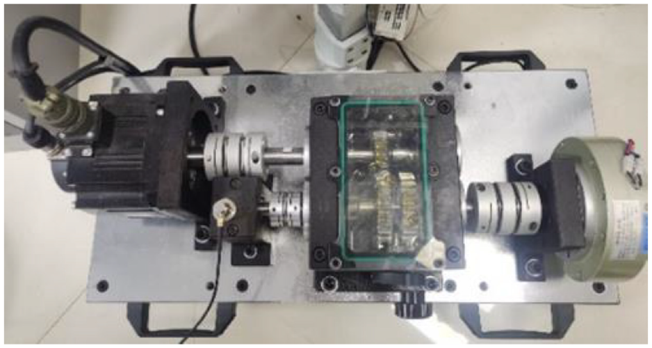
Self-built test rig.
The vibration signals in vertical and horizontal directions are collected by two accelerometers installed on the upper right surface of the bearing test motor attached with a sampling frequency of 2.56 kHz. The bearing failure type involves a defect with a depth of 0.5 mm and a width of 0.2 mm. Detailed information on the SBTR dataset is listed in Table 5.
Details of the SBTR dataset.
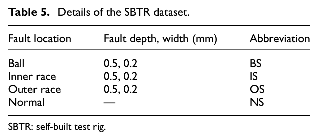
SBTR: self-built test rig.
To establish a clear distinction, the sampling point value in the SBTR dataset is set to 4200. Then, the raw vibration signals are converted into time-frequency images, as shown in Figure 17.
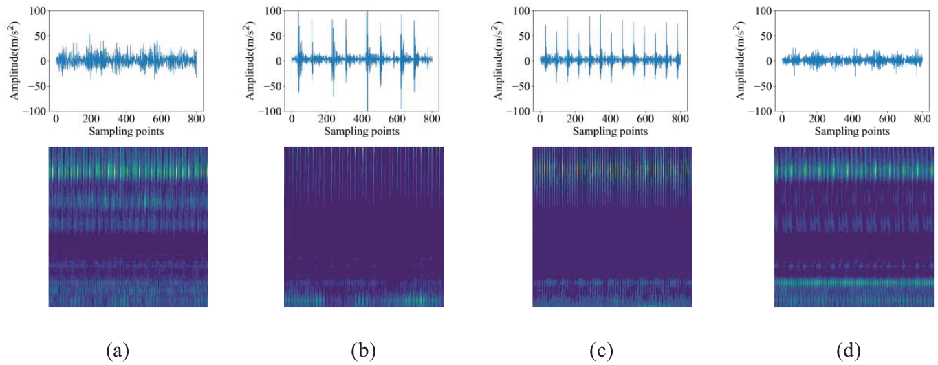
Time-frequency images of four states on the SBTR dataset: (a) BS, (b) IS, (c) OS, and (d) NS.
Comprehensive performance evaluation of SFGAN-TDTL
On the SBTR dataset, the time consumption and image quality of various GANs are added to the comparison. The three-dimensional axes representing SSIM value, FID value, and data generation time are shown in Figure 18.
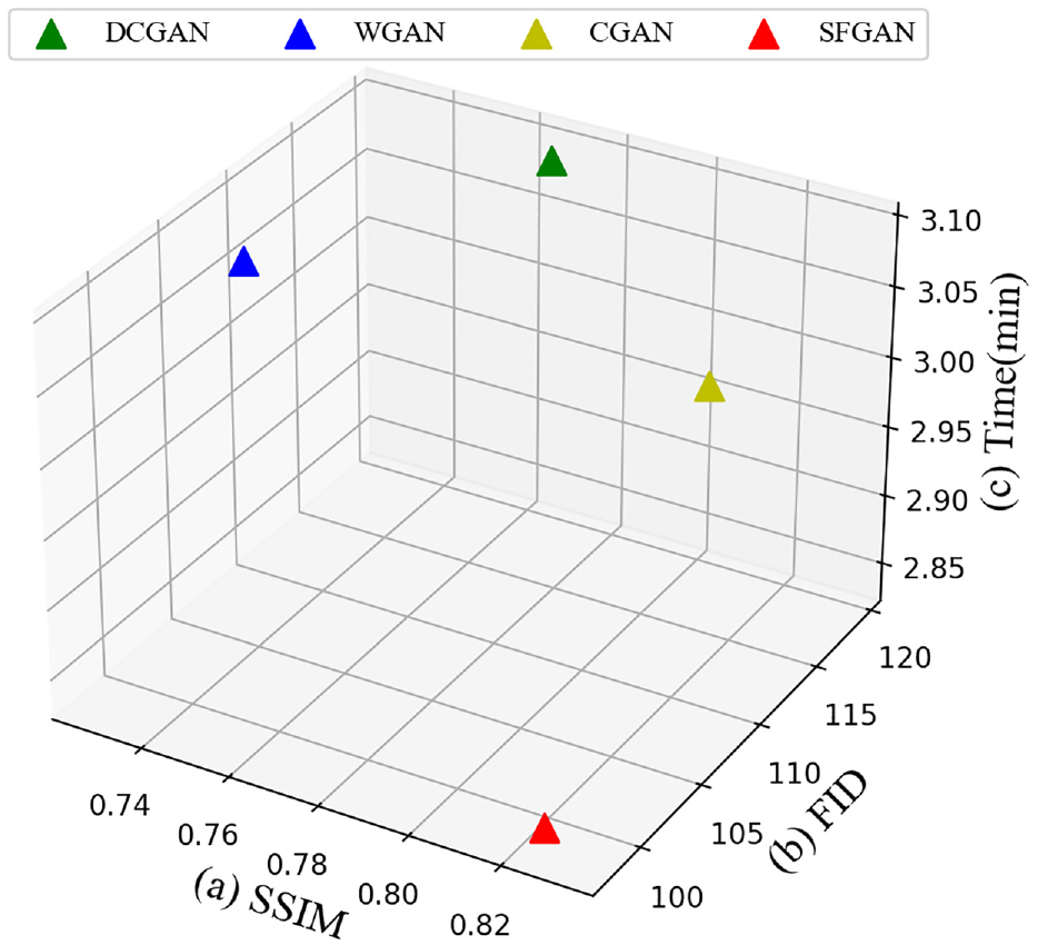
Comparison of different GANs on three indicators: (a) SSIM, (b) FID, and (c) data generation time.
As shown in Figure 18, SFGAN reaches the best balance between image quality and data generation time. Finally, we conducted comparison experiments to assess the time consumption and diagnostic accuracy of different GAN-based fault diagnosis methods. These experiments are performed on the SBTR dataset, and the results are shown in Figure 19.
Performance comparison on the SBTR dataset: (a) Training time; (b) Accuracy.
In Figure 19, the time consumed by the SFGAN-TDTL is approximately half that of the other comparison methods. Due to its excellent performance in both diagnostic accuracy and time consumption on the CWRU and SBTR datasets, SFGAN-TDTL exemplifies the potential to save time.
Conclusion
Accurate fault pattern recognition is a crucial task in bearing fault diagnosis, and various approaches have been proposed. In this study, a bearing fault diagnosis framework named GAN-DTL is proposed. GAN is employed to generate synthetic data, while DTL is utilized for weight transfer and fine-tuning. Building upon GAN-DTL, a time-saving fault diagnosis approach, called SFGAN-TDTL, is proposed. First, SFGAN is proposed to reduce the time consumption of data generation, leveraging the LSC module with 1 × 1 convolution and skip connection. Subsequently, TDTL is proposed to reduce training time based on open-source data, synthetic data, and real data. Experimental results have demonstrated that the SFGAN-TDTL method can achieve high diagnostic accuracy with small samples while significantly reducing time consumption.
Footnotes
Declaration of conflicting interests
The author(s) declared no potential conflicts of interest with respect to the research, authorship, and/or publication of this article.
Funding
The author(s) disclosed receipt of the following financial support for the research, authorship, and/or publication of this article: This work was supported by National Natural Science Foundation of China under Grant No.52305125 and No.51875416, Hubei Natural Science Foundation Innovation Group Program, Youth Program, and Innovation Development Joint Key Program, under Grant No.2020CFA033, No.2023AFB028, and No.2023AFD001, respectively, Wuhan Key Research and Development Plan Artificial Intelligence Innovation Special Program under Grant No.2023010402040005, and 14th Five Year Plan Hubei Provincial Advantaged Characteristic Disciplines (Groups) Project of Wuhan University of Science and Technology under Grant No.2023B0301, which are greatly appreciated.