
Abstract
Accurate modeling of guided wave propagation is crucial for structural health monitoring (SHM) systems, where a large amount of information and cases are needed to cover all in-service conditions of a structure. Finite-element models have proven to be accurate enough to simulate the problem; however, they typically require substantial computational resources, and each simulation may require a significant amount of time. This article presents a comprehensive study of a ray-tracing-based wave propagation methodology applied to predict the acoustic behavior of lightweight structures. Focused on composite materials, particularly carbon fiber-reinforced plastic (CFRP), the study addresses the growing need for accurate and fast simulation tools in industries where high-strength lightweight materials play a pivotal role, such as aerospace or automotive. The study presents an examination of the ray tracing method’s effectiveness with series of experimental coupon tests, ranging from a simple metallic plate to a representative CFRP wing lower cover of the Universidad Politécnica de Madrid-LIBIS Unmanned Aerial Vehicle. The investigation spans a distribution of possible damage locations ensuring a comprehensive applicability evaluation. Results demonstrate efficacy in predicting the wave propagation characteristics, including transmission, reflection, and absorption within composite structures, and also an accurate representation of its behavior for in-service damages, both via added masses and real impact damages. The validation involves an in-detail comparison with experimental measurements, evaluating the reliability and applicability of the ray tracing approach. This research not only contributes to the advancement of predictive modeling for acoustic behavior in composite structures but also addresses the broader implications for industries relying on accurate simulations for design optimization and performance evaluation. The validated ray tracing method has proven to be a valuable tool to ensure precise predictions of wave propagation in composite materials, and its computation speed makes the methodology ideal to contribute to a training database for a possible physics-informed machine learning SHM system.
Introduction
Structural health monitoring (SHM) performs a crucial function in industries where lightweight, high-strength materials are essential for achieving optimal performance and efficiency. These structures, and specifically carbon fiber-reinforced plastic (CFRP), can present a much wider range of specific failure modes, such as delaminations, fiber breakage, matrix cracking, and impact-induced damage, some of which may be difficult to assess by visual inspection.1–4
SHM works by employing various sensing technologies, data acquisition systems, and signal processing techniques to be able to monitor the structure periodically or in real time. There are two primary approaches in the field: data-driven and model-driven. 5 Data-driven methods are supported directly on structural data, from which they are able to deduce the normal operational state of a structure typically using machine learning processes. On the other hand, model-driven methods leverage simulations to ascertain the health condition of a structure by directly comparing the models’ predictions with the actual structural information taken from the sensors. 6
The extraction of damage-sensitive features from the structure and the analysis of these features can be used to detect, quantify, and determine the location of damage and, additionally, the system could be used to capture real-time events and assess them, 7 or even be able to consider even the effect of corrosion 8 and other environmental factors. 9
To achieve this, every kind of methodology must be fed with data from a sensor network, which must be permanently installed in the structure. There are many kinds of sensors currently available in the industry, and in this article, we focus on ultrasonic inspections, which have historically proven to be a reliable and cheap way of evaluating manufacturing defects or in-service damages. This technique is ideal for lightweight structures, as elastic waves are able to travel large distances with very low attenuation and are very sensitive to typical damages of interest 10 in both metallic and composite materials. 11
A significantly complex structure could, therefore, be inspected with a very small number of sensors12,13; employing elastic waves with a distributed piezoelectric actuator/sensor network based on the pitch-catch method has proven to be very successful for impact damage detection14,15 and even for other nontypical damages such as crack and corrosion localization. 16 These SHM systems could present many cost advantages when compared with the traditional inspection methods and could also be used to improve the life prediction of the structure based on its usage.13,17
Being able to extract relevant damage identification parameters and accomplish the objective of these systems still requires a significant effort in terms of signal analysis and interpretation18,19 and must be substantiated by relevant testing experience. However, due to the high cost of physical tests, numerical simulation can be especially helpful to predict the elastic wave propagation and may help improve the accuracy of these systems. 20 These data-driven methods, also referred as physics-informed machine learning systems, are an emerging methodology that can also significantly aid in the interpretation of SHM data. The basic idea consists in combining physics-based models with data-driven ones taking advantage of both to improve predictive capability in an SHM setting. 21
Numerical simulations provide a very effective way to capture and understand the structural behavior in terms of elastic wave response; general-purpose computational codes such as time-domain spectral finite-element methods22,23 or explicit finite-element methods20,24–26 are commonly used to calculate the wave propagation and have proven to be a useful tool when used for training of a physics-informed machine learning model. 27
Finite-element or finite-difference methods could still present a series of significant disadvantages that may still render them not suitable to be used in some SHM system applications. Some of the most limiting ones could be:
Computational complexity: the methodologies tend to be computationally intensive, especially for large and complex structures. Long computation times and high memory requirements may limit their efficiency and are usually not suitable for real-time or iterative analyses.
Grid or element discretization: discretizing the structure into grids or elements may result in some loss of accuracy, difficulties in capturing fine details, or aliasing effects on high frequencies. The choice of grid or element size can impact the accuracy and computational cost of the analysis and is usually a limiting factor for the maximum scale of structures to be analyzed.
Material damping of boundary damping: specifically for the explicit finite-element method, introducing damping elements, either as dashpots or material damping, significantly reduces the stable time increment, making it exponentially more costly to solve problems where this effect is relevant on the solution.
For these reasons, and also to increase the reliability of the simulations, there have been multiple attempts of solving the problem without resorting to finite elements in the literature, either analytically28–30 or using statistics or artificial intelligence31,32; some of these methods are able to achieve very good results, but the algorithms studied tend to be too complex to generalize or limited in applicability.
There are, however, other numerical approaches that may breach the problems issued above; specifically, this article focuses on the ray tracing method, which is based on the assumption that the particle motion can be modeled as a number of idealized narrow beams (rays) advanced through the medium by discrete amounts. Tracing the paths of individual rays provides valuable information about wave behavior, including wavefront curvature, mode conversion, reflection, and transmission as the rays interact with the objects present along their path. Ray tracing methods have been extensively developed recently for graphics rendering due to the recent technological developments of high-end graphics cards, 33 but have also been continually used historically for science and research in different fields such as astronomy 34 or optical design. 35
Ray tracing, however, is not limited to visual rendering, as it can also be applied to simulate sound propagation in various environments. In the context of acoustics and sound engineering, it involves tracing the paths of sound waves as they interact with the boundaries given by the structure. This technique allows for the modeling of how sound behaves in complex 2D or 3D environments, considering factors such as reflection, diffraction, and absorption.
The ray-tracing-based approach offers significant advantages over traditional numerical methods in terms of computational efficiency and ease of implementation as it is not limited by an element size, although a large number of rays may be limiting in some applications. It provides a practical tool to analyze wave propagation phenomena and has been widely used in scientific research for many different applications, most notably: ocean acoustics36,37 or heat transfer. 38
Specifically, it has also been previously used in SHM to solve the guided wave propagation problem, and it has proven its effectiveness, tracing possible reflections individually implementing a multipath baseline-free damage imaging method, 39 applying it to iterative tomography to reconstruct Lamb wave velocity maps, 40 using two-step algorithms to identify possible propagation paths and computing the sensors signals, 41 tracing reflections from an initial ray beam in in-homogeneous media, 42 or even to aid in the interpretation of experimental results. 43
The solution presented in this article also applies the ray tracing method to solve the general guided elastic wave propagation problem for an arbitrary 2D structure, and it aims to provide additional versatility such as accounting for multiple sensors or actuators and adjustable boundary parameters in order to accurately match experimental data, with the objective of developing an efficient and accurate numerical model that may be later used as part of a complete SHM framework, whether it is to train an artificial intelligence model or to determine relevant damage indicators.
Additionally, the sensor model developed considers a finite area instead of a single spatial point. This provides a significant advantage when compared with other ray tracing methodologies as it eliminates the need of computing eigenrays, and the sensor size and geometrical dispersion are considered intrinsically.
The main limitation of this approach is that a sufficiently large number of rays must be used to completely capture all possible relevant propagation paths that may reach the sensor, analogous to the number of elements or nodes on an explicit finite-element model (FEM), although its computation is still significantly more efficient.
In order to validate the methodology and demonstrate its applicability, the article is structured in the analysis of a series of case studies. First, a metallic rectangular aluminum plate is used as an initial validation for an isotropic material and the ray tracing results are compared with an FEM simulation. This specimen is also used to adjust the boundary reflection parameters of the simulation.
Afterward, the simulation is then validated against a representative composite structure, corresponding to the wing lower cover of the experimental LIBIS Unmanned Aerial Vehicle (UAV). Artificial damages are introduced in the structure adding small masses using vacuum paste, and the test results are compared with the simulation.
Finally, the simulation is validated with a real damage present in the structure. An impact of 7 J generating of a possible representative barely visible impact damage (BVID) is performed in the LIBIS composite wing. The damage is inspected with traditional Nondestructive Testing (NDT) techniques and with the installed Lead Zirconate Titanate (PZT) sensor network and compared with the simulation results. This is shown in a qualitative way by comparing the Hilbert transform of the signals.
Materials and methods
The basic idea behind ray tracing involves tracing the path of straight ideal rays as they travel through the structure. This process simulates the behavior of these ultrasonic waves considering factors like reflection, refraction, dispersion, and, indirectly, shading. The main steps involved in the analysis are as follows:
The refracted ray path along the structure is governed with the Snell’s law and, at the boundary of two mediums 1 and 2, is expressed as:
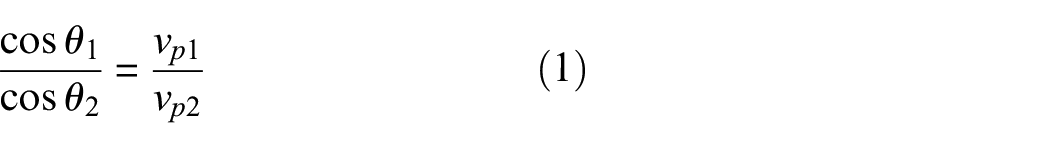
where
When a ray encounters a boundary, a component of the ray energy is reflected and another part is refracted or transmitted. For the particular case in which the ray would reach a segment end (i.e., a corner), the ray is eliminated from the model. This approach is taken as a simplification to reduce computational effort, as the effect is negligible for a sufficiently large number of rays and can be minimized considering initial rays that will not intersect any corners of the model on their first propagation step, for example: by choosing an odd number of initial rays.
The model takes into account the mode conversion phenomena44,45 at each boundary, and therefore, the transmitted and reflected component energy is divided between the different propagation modes.
The energy of the incident ray

where
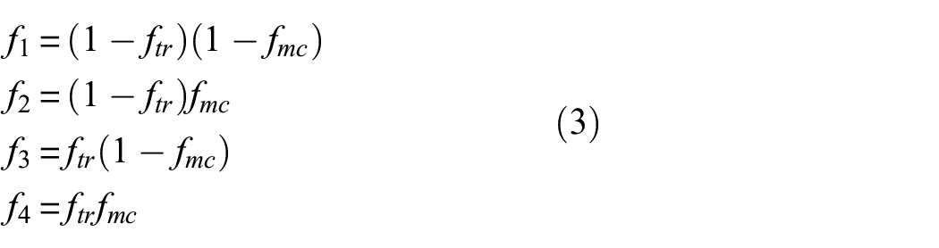
considering
Wave speed and dispersion in metals
Wave propagation in isotropic plates, such as metals, can be understood by the characteristic Lamb wave equations, initially established by Horace Lamb in 1917 and further developed by Raymond Mindlin in 1951.
46
They define group and phase velocities for waves propagating in an infinite plate, describing two modes of propagation: symmetric
These equations were derived by setting up formalism for a solid plate having infinite extent in the x- and y-directions and thickness
Lamb wave equations originate from imposing sinusoidal solutions to the wave equation; they have no analytical solution and must be solved iteratively to estimate the wave propagation speed at any given frequency–thickness ratio. The equations intrinsically imply that Lamb waves are dispersive regardless of propagation mode, resulting in a frequency-dependent speed. The main parameter that governs the dispersive behavior of the waves is the ratio of plate thickness h to wavelength
As the problem is formulated by assuming an infinite plate, by definition, Lamb waves have no particle motion in the y-direction. Motion in the y-direction in plates is found in the so-called
Wave speed and dispersion in composite materials
Composite materials present characteristic anisotropic stiffness properties that have a significant influence on the propagation speed and media dispersion for elastic waves. 48 The stiffness transfer matrix method has proven to be a good approximation in order to estimate the wave propagation speed 49 ; this methodology is well suited for multilayered media as it condenses the system into four equations, eliminating all other intermediate interfaces. It can be calculated for each medium before the tracing of the ray propagation map and the propagation speed of each individual ray can be later interpolated from it based on its traveling direction angle and wave mode.
Assuming that all composite layers behave as orthotropic media and following Hooke’s law generalized for a two-dimensional shell, the layer stiffness matrix expressed in the laminate coordinates (rotated around the laminate perpendicular axis)
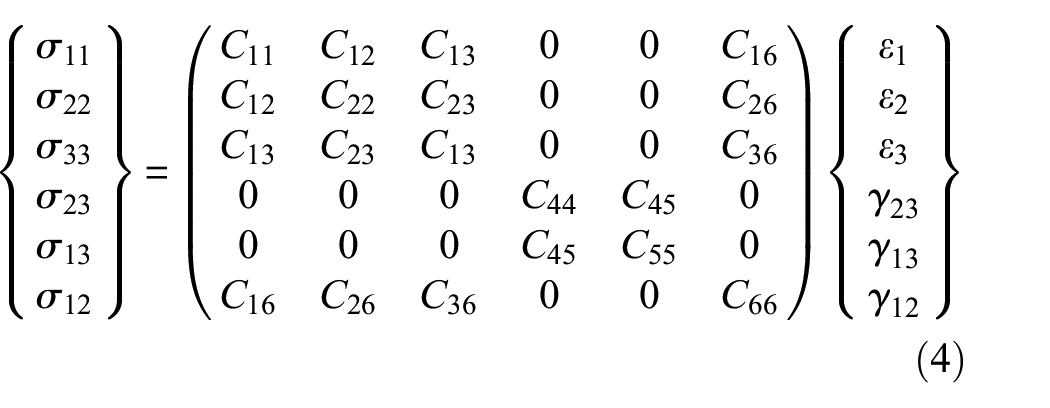
where
Applying Newton’s second law to the stiffness matrix from Equation (4) and considering the small linear strain displacement approximation, given by:
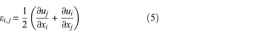
the internal forces can be converted into internal stresses, resulting in
where
Therefore, the equations of motion can be rewritten in matrix form as:
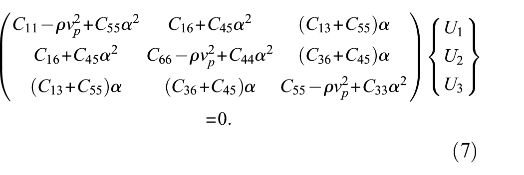
The system from Equation (7) can only present a nontrivial solution when its determinant equals zero; therefore, it could be studied as an eigenvalue problem to obtain the values of
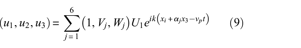
Once solved, the values of

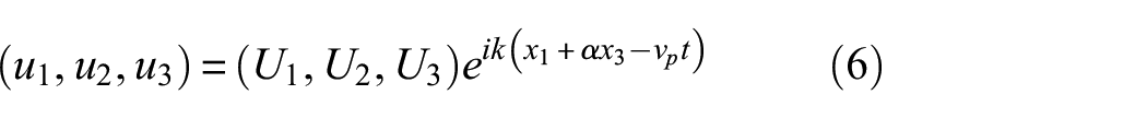
It is then possible to rewrite the expressions for displacements and layer stresses as a function of
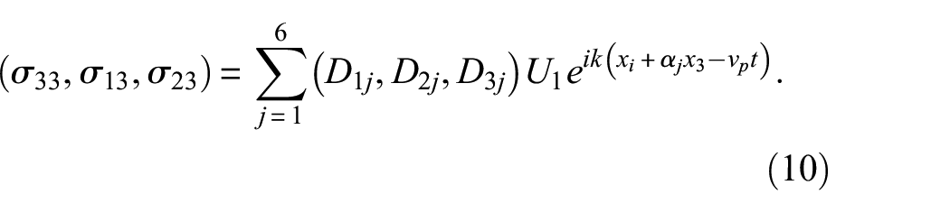
Values for the matrix terms
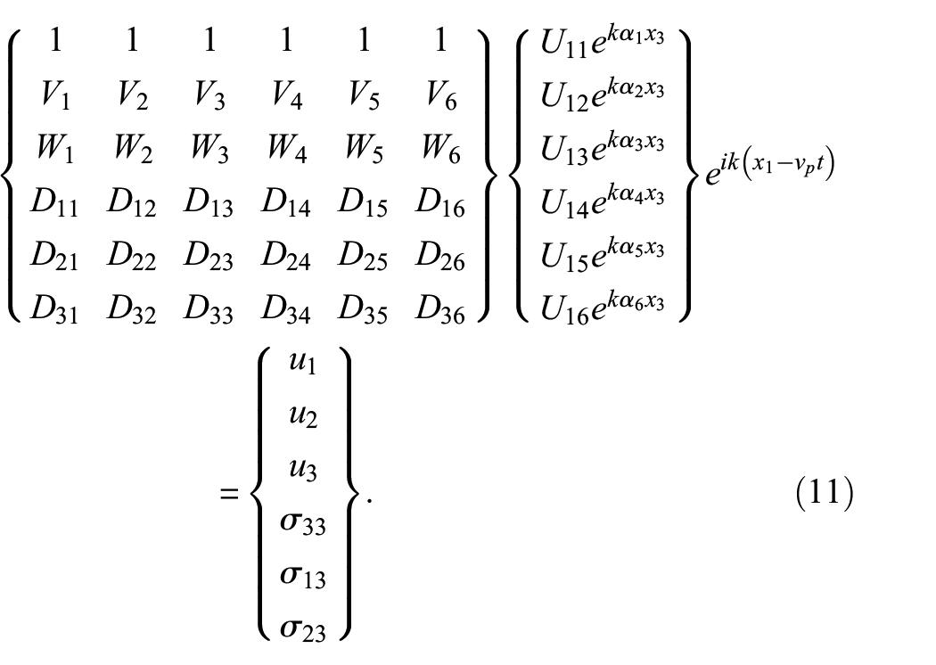
Guaranteeing continuity by solving Equation (11) at the top and bottom of each layer, it is possible to obtain a relation between the upper and lower surfaces of the plate. Therefore, for a laminate of
Stress-free boundary conditions are then guaranteed in the top and bottom layers as
While the phase velocity,
In a dispersive medium, where different frequencies of a wave travel at different speeds, the group velocity
The shear wave propagation mode
Ray signal recovery
In the case of active interrogation, a tone burst is typically used as an excitation signal, usually consisting of a 10 – 50 V peak-to-peak sine wave modulated by a Hamming window. These signals are named with the convention BURSTn where
The signal information is carried independently on each ray in the frequency domain, via a sufficiently large amount of terms of their Fourier transform, and could then be altered as the ray propagates through the model due to different effects, such as material damping which is considered as a factor over the signal amplitude

where
The signal is then recovered at each point applying the time shift property of the Fourier transform:

As the signal is dispersive, the phase velocity as a function of frequency
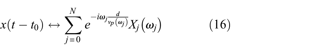
where d is the distance along the ray path where the signal is to be obtained.
The ray tracing implementation is designed to be used with piezoelectric transducers, as these sensors are ideal for SHM systems due to their low weight and their ability of both generating and measuring guided elastic waves. Piezoelectric wafers tipycally low-cost and lightweight and can be used for active sensing of far-field damage using pulse-echo, pitch-catch, and phased-array methods.
Nonetheless, as signals obtained in this sensors unavoidably contain multiple modes, it is required to use complex signal processing techniques to extract useful information.
To include the PZT sensors in the simulation, they are modeled as a circle boundary. This boundary does not interact with the incident rays; however, the intersection time points (
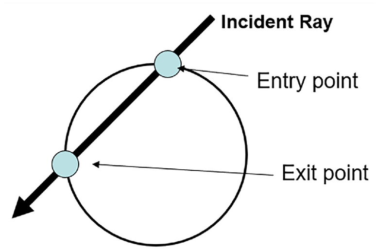
Schema of the PZT sensors model for the ray tracing algorithm.
There are a number of significant advantages that arise from using this methodology, the main one is being able to avoid the need to calculate eigenrays to the sensors or to use a two-step methodology by using focused ray beams and locating the paths to the sensors. Instead, the solution is solved by a single iteration, where the transducer emits rays in all directions and all relevant propagation paths could be captured by the sensor with a sufficiently large number of initial rays.
As the sensors act as a signal integrator, the geometrical spreading effect is inherently captured by modeling its area and adding up all the rays that intersect the sensor on their path; with a sufficient number of rays, the effect converges to the analytical geometrical spreading predicted by the wave equation. In addition, the sensor size is taken into account, and its effect, which is significantly more relevant for cases where the signal wavelength is comparable to the sensor dimensions, can be evaluated with this methodology.
On the contrary, a larger number of initial rays are needed to achieve a good solution, and later reflections may be captured imprecisely or not be captured at all due to the low number of rays that may cross the sensor, although this could be solved by iteratively increasing the number of rays until achieving a converged solution.
PZT transducers may reveal certain nonlinear behavior and hysteresis under large strains/voltages or at high temperature; implementing this in the simulation could be done by applying a transfer function directly modulating the resulting sensor signal; however, as the experimental set does not reflect this behavior, it is not studied in this article, and it is assumed that all components of the acquisition systems function in their linear range. Other phenomena that may be exhibited by these transducers such as brittleness, low fatigue life, etc. 52 are also not reflected in the proposed methodology and may limit its application range.
Isotropic metallic plate analysis and methodology validation
The methodology is first validated against a physical test in a rectangular aeronautic grade 2023-T3 aluminum plate. The test is instrumented with an array of 7, evenly distributed, piezoelectric sensors (8-mm PZT ceramic wafer, over a 12-mm bronze disc), and the data are recorded with an Acellent SCAN GENIE system, with a sampling frequency of 48 MHz. The plate is simply supported on two of its sides. The support effect is considered negligible for the simulation, and it was opted to just assume a constant uniform energy loss in all of the boundary; weight of cabling and instrumentation are also not considered in the simulation (Figure 2).
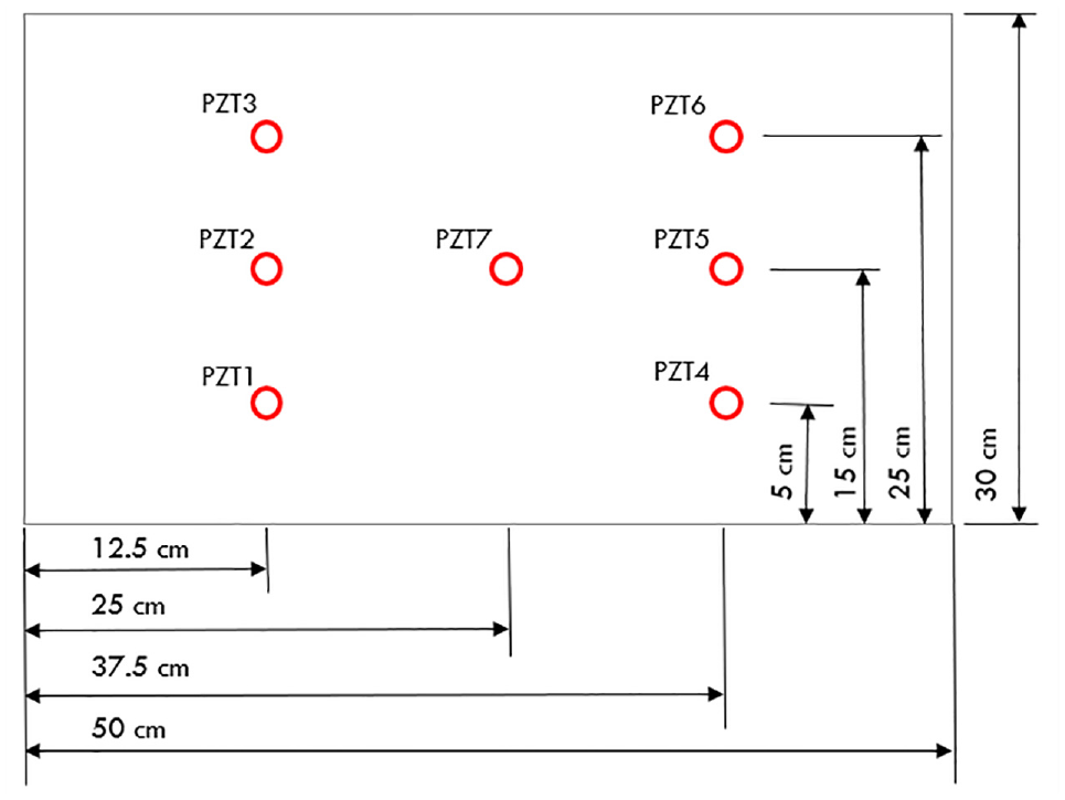
Schema of the PZT sensors location for the metallic plate study.
The results of a ray tracing simulation, for 1602 initial rays (801 S0 rays and 801 A0 rays), are shown as a heat-map in Figure 3(a) at a time
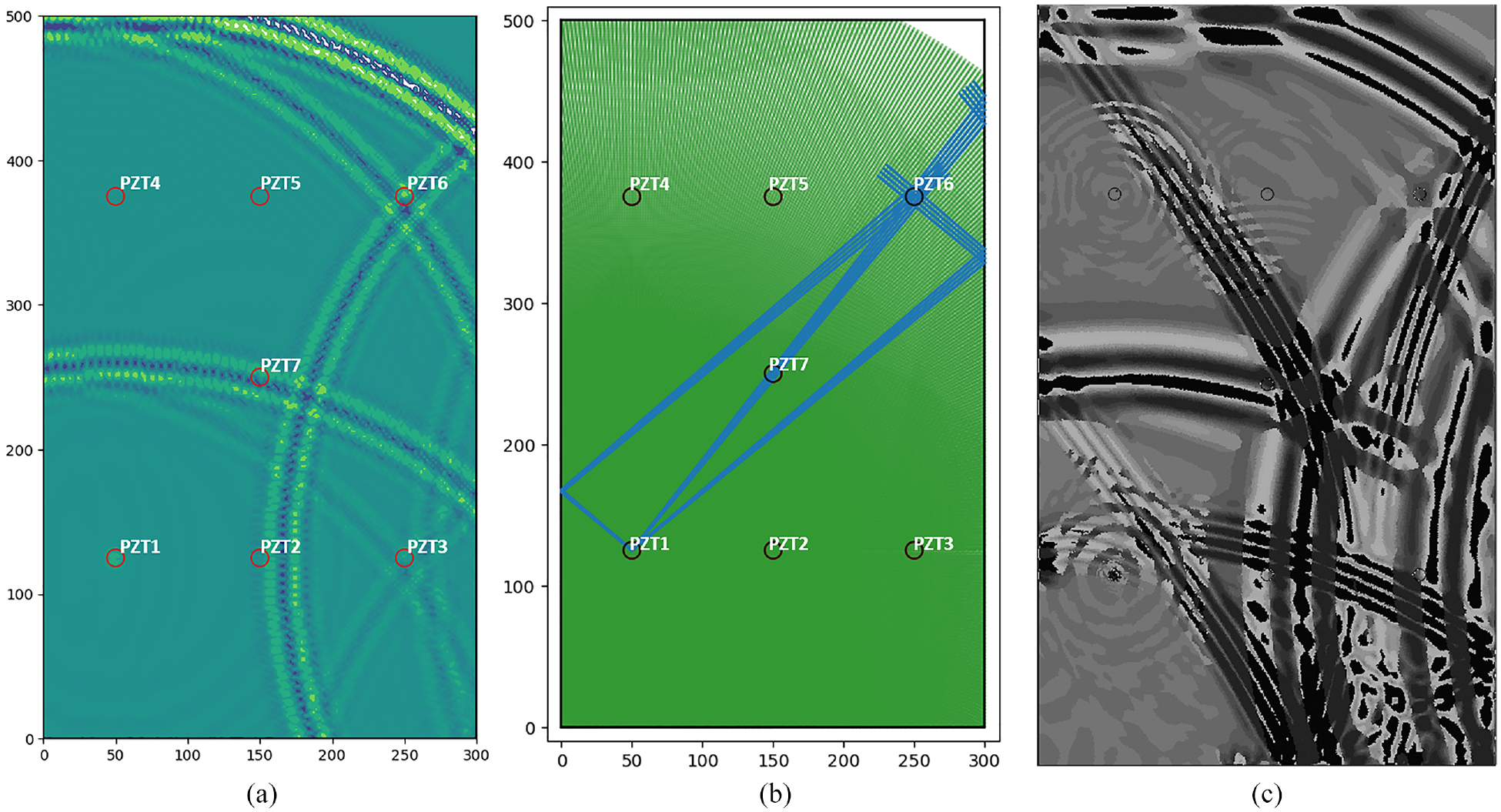
Simulation results (FEM and ray tracing) at
These results are compared with a dynamic explicit time integration FEM, run in Abaqus/Explicit version 2020 HF6, that has been developed to aid in the ray tracing validation, following the modeling principles described in Sánchez Iglesias et al. 53 A contour plot of the absolute maximum principal membrane strains is shown in Figure 3(c).
In order to simulate a 300-kHz elastic wave, the element size is limited to approximately 1 mm, resulting in 539 reduced integration shell elements, S4R, for the transducers and 370,235 reduced integration continuum shell elements, SC8R, and a total of 185,144. The stable time increment of the FEM simulation is
The heat-map shown in Figure 3(a) is calculated by mapping the rays signal over a square grid with a characteristic length of 2 mm. The figure shows how the elastic waves propagate through the plate and interact with each boundary and how the energy is being dissipated after each reflection.
In order to capture the results on a selected transducer, the rays that intersect the sensor must be detected and integrated over its length. As an example, all rays captured by transducer
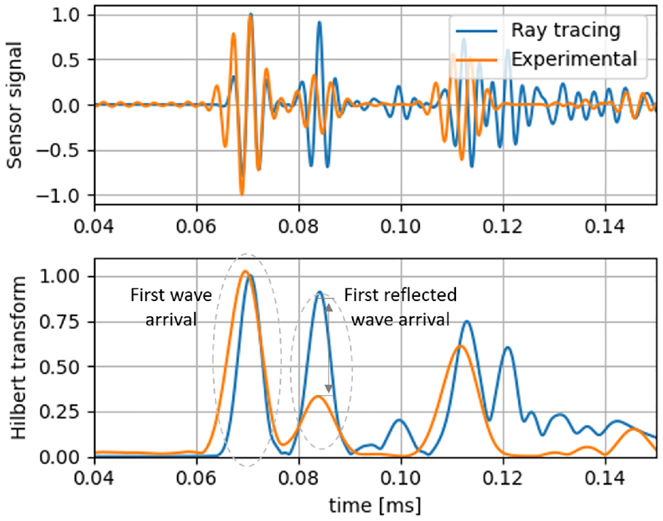
Result signal and Hilbert transform for path 1-6, normalized with first wave arrival amplitude peak.
In order to better interpret signal results, they are compared both as-is and in terms of their Hilbert transform. An analytic signal is defined in terms of a real part and an imaginary part; its magnitude is related to the magnitude spectrum, and its phase angle its phase spectrum. Features, such as standard deviation of amplitude, standard deviation of phase, and signal energy, can be extracted from these spectrums.
The real and imaginary parts of the analytic signal are related by the Hilbert transform, which takes a function
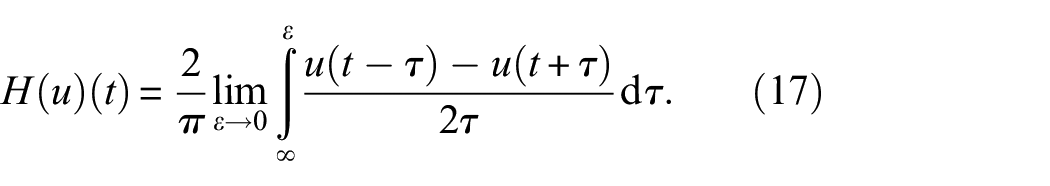
By taking the real function
The absolute value of the Hilbert transform gives a representation of the instantaneous amplitude of the function, as shown in Figure 4, where it is plotted alongside the sensor signal to aid with its visual interpretation.
As shown in Figure 4, the intensity of the first peak of the received signal is related to the amplitude of the input and material properties (damping or guided wave dispersion) during the wave path. Its absolute value, however, is governed by many different factors such as piezoelectric characteristics of the sensors or the amplification factor of the acquisition system. These factors, although, out of the scope of this study, are assumed to have a linear effect on the signal, and therefore, the experimental signal is normalized when compared with the simulated data.
Second and successive peaks on the received signal are related to wave reflections on the plate edges (the A0 wave arrives at the sensor significantly later and at a point where its distinction from other phenomena is not clear from the experimental signal due to its relatively low propagation speed in this condition). Their relative amplitude is, therefore, governed by the energy dissipated in those reflections. This is taken into account in the simulation by the boundary losses coefficient set at the edges .
A parametric study is performed evaluating the boundary losses coefficient
The normalized error on the second peak resulting of this study is shown in Figure 5, along with its average and standard deviation for each of the sensor paths present in the plate. The average of each measure is joined together to highlight the tendency of the data.
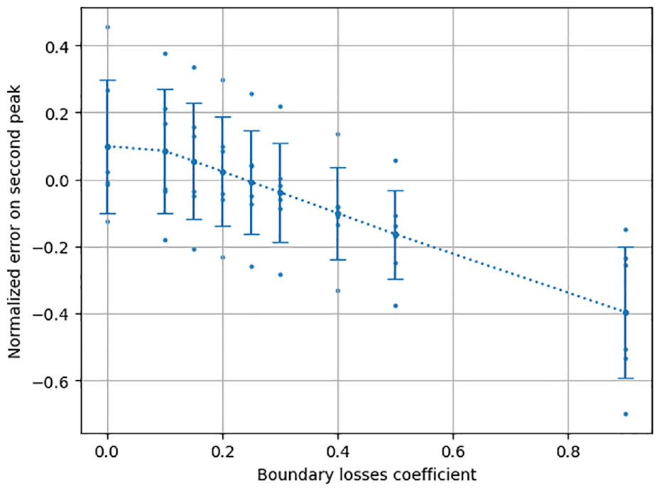
Aluminum plate error on second peak.
Figure 5 shows a significant dispersion in the data; this dispersion has been mainly attributed to factors not accounted for in the simulation, such as precission in sensor position and adhesion to the plate, plate material imperfections, sensors and cabling weight, and differences in the edges and supports of the plate, which are only represented in the simulation as the uniform factor
Therefore, based on the results of this study, the boundary losses factor
The results obtained for a number of relevant paths are shown in Figure 6 compared with the experimental test results and the FEM results, for a simulation with 1602 initial rays and assuming the boundary losses factor
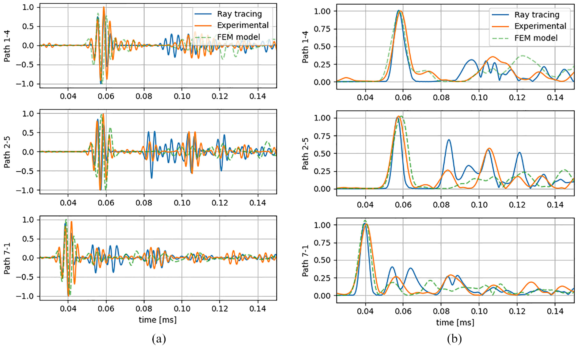
Signal intensity comparison for relevant sensor paths, normalized with first arrival amplitude peak: (b) raw signal and (b) Hilbert transform.
As shown in Figure 6(a) and (b), the simulation presents a very good agreement with the experimental data after the boundary losses coefficient fitting, for all configurations explored. Initial wave packet and reflections appear with precision both in arrival times and amplitude in the simulation results, although some differences can be observed on some of the later reflections that may be explained due to signal error accumulation, sensor positioning and bonding imperfections, geometrical differences or imperfections in the boundaries, materials and sensors, and cable and sensors’ weight.
The correlation with the tests shown in Figure 6 obtained by the ray tracing method is comparable in accuracy to the FEM simulation, and most of the possible sources of error identified are applicable to both methodologies.
A computation time comparative is shown in Table 1. Both computation times of the signal at one sensor,
Computation time comparison: FEM versus ray tracing.
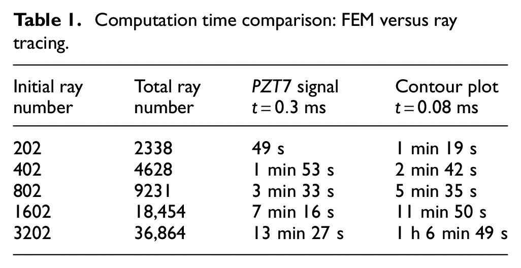
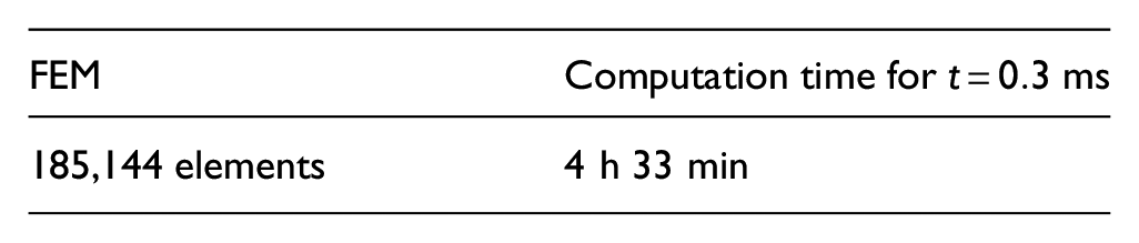
For comparison, the contour plot is performed with a grid length of 2 mm, consistent with the plot shown in Figure 3(a). The ray tracing model runs a single processor on a standard work laptop (Intel Core i7-10875H CPU@2.30 GHz) and the FEM runs on four processors on an HPC cluster (Intel Xeon Gold 6136 CPU@3.00 GHz).
It is clear from the results shown that the ray tracing method provides a significant time advantage over the FEM (considering the examples used for the method validation of 1602 initial rays, the time difference is nearly of two orders of magnitude); moreover, pre- and postprocessing times of the FEM are not considered in the results shown; however, for a model of this size, this could become a significant time investment.
However, the ray tracing methodology requires the adjustment of a larger number of parameters than the FEM, especially in the presence of geometrical boundaries. Nonetheless, the advantages in computation time are very significant, making the ray tracing method especially attractive for generating a large number of data points that could be used in cases of artificial intelligence training databases.
Study of artificial damages on composite wing demonstrator
In order to evaluate the simulation behavior in the presence of damage, the methodology is compared against a physical demonstrator of the front left wing lower cover of the remotely piloted aircraft system LIBIS, designed and built by the Technical University of Madrid (Figure 7).
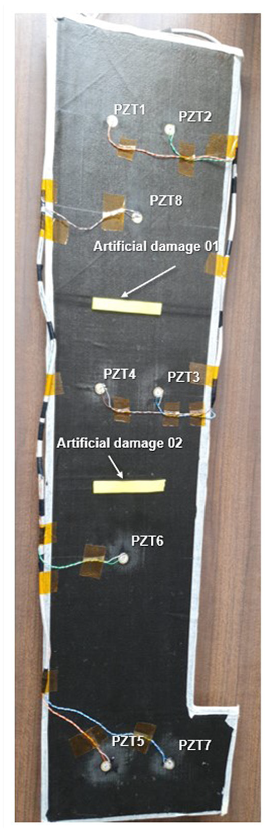
Example test configurations evaluated on LIBIS wing prototype. Transducers and artificial damages location and numbering.
The specimen is instrumented with an array of eight piezoelectric transducers (8-mm PZT ceramic wafer, over a 12-mm bronze disc), shown in Figure 7, and the data are again recorded with the same Acellent SCANGENIE system, using a sampling frequency of 48 MHz.
Artificial damages have been introduced in the specimen, as shown in Figure 7. They are introduced with 8-cm-long, 1-cm-thick strips of vacuum paste stuck on the inner side of the laminate, with an average mass of 5 g; they function as added masses in order to alter the dynamic behavior of the structure. Given that the structural integrity of the CFRP remains intact under the vacuum paste, it is considered that the effect of adding the masses could show a higher resemblance to the effect of a delamination or matrix failure rather than a fiber breakage, although other types of damages may have a similar effect.55,56
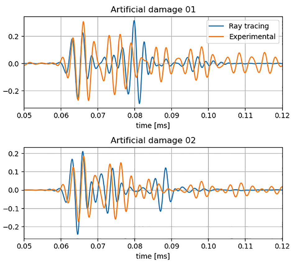
Three sets of tests were performed considering the intact structure, the structure with artificial damage 01, and the structure with artificial damage 02. The input signal used consists of a 40-V BURST3 at 350 kHz, and test results are presented as an average of three runs; these parameters are not a limitation of the simulation method; instead, they are selected based on the best experimental result data available.
A contour plot of the simulation results for each case is shown in Figure 8 at
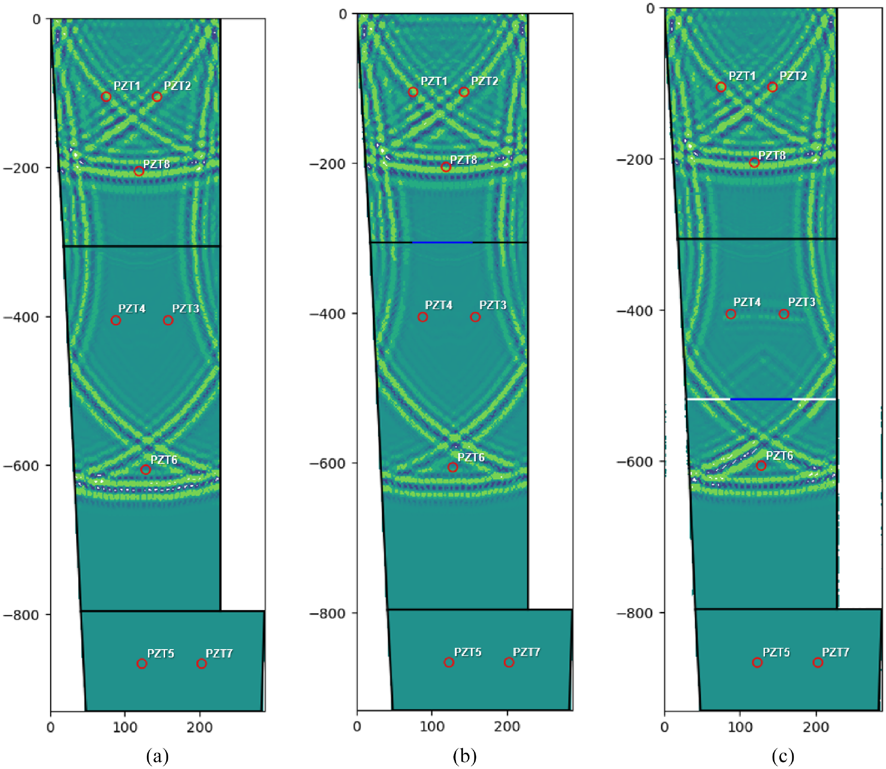
Numerical result contours for the configurations evaluated on LIBIS wing prototype, at
In order to quantify the effect of the damage on the system, both the energies reflected and dissipated in the artificial boundary were adjusted manually based on the shortest linear propagation path, in this case corresponding to between sensors
The raw signal obtained with the tests is compared against the simulation in Figure 9 for the path between
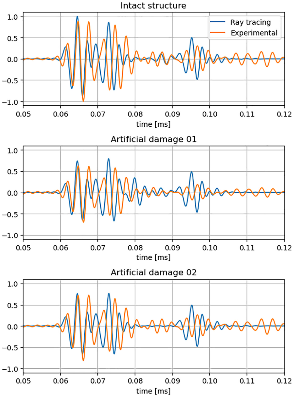
Simulation versus test results’ raw signal comparison with artificial damages for path 8-6, normalized with first wave arrival amplitude peak.
Scattered wave signal (the difference between intact and damaged signals) is shown in Figure 10, for the path between
Simulation versus test results’ scattered wave signal comparison with artificial damages for path 8-6.
Although in this case there are much higher uncertainties in the experiment and the differences between test and simulation are more significant than in the metallic plate case, the model predictions are still consistent with the experimental data when estimating the effect of the artificial damages on the signal, and its effect can be observed and quantified with the sensor network data.
Real impact damage study on composite wing demonstrator
Evaluating the effect of a real damage on the LIBIS panel is then subjected to a 7 J impact, with a 1-kg-steel 20-mm-diameter spherical tip impactor, using a 70-cm-tall drop tower. The impact is located in the center of the panel in a similar location as the artificial damage 02, at approximately 6 cm from the lower cover trailing edge. The impact is performed on the outer face in order to emulate a possible real BVID due to some external in-service damage.
Images of the resulting impact are shown in Figure 11. As expected, the effects of the damage can be more clearly observed on the opposite side of the impact, appearing as some fiber breakage, shown in Figure 11(b), while on the impact side (Figure 11(a)), they appear only as a small indentation.
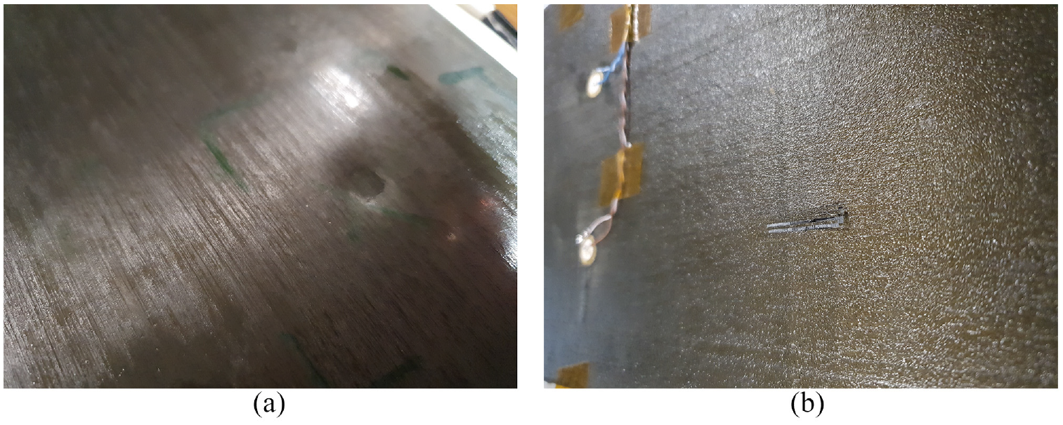
7 J impact damage pictures: (a) impacted side and (b) opposite of impacted side.
To fully characterize the impact, the damaged area is inspected with an Olympus OmniScan MX2 and its results of the A-, B-, and C-scan are shown in Figure 12, where significant delaminations and fiber and matrix crackings spanning an approximate area of 23 cm2 and extension of the damage through the complete plate thickness can be observed.
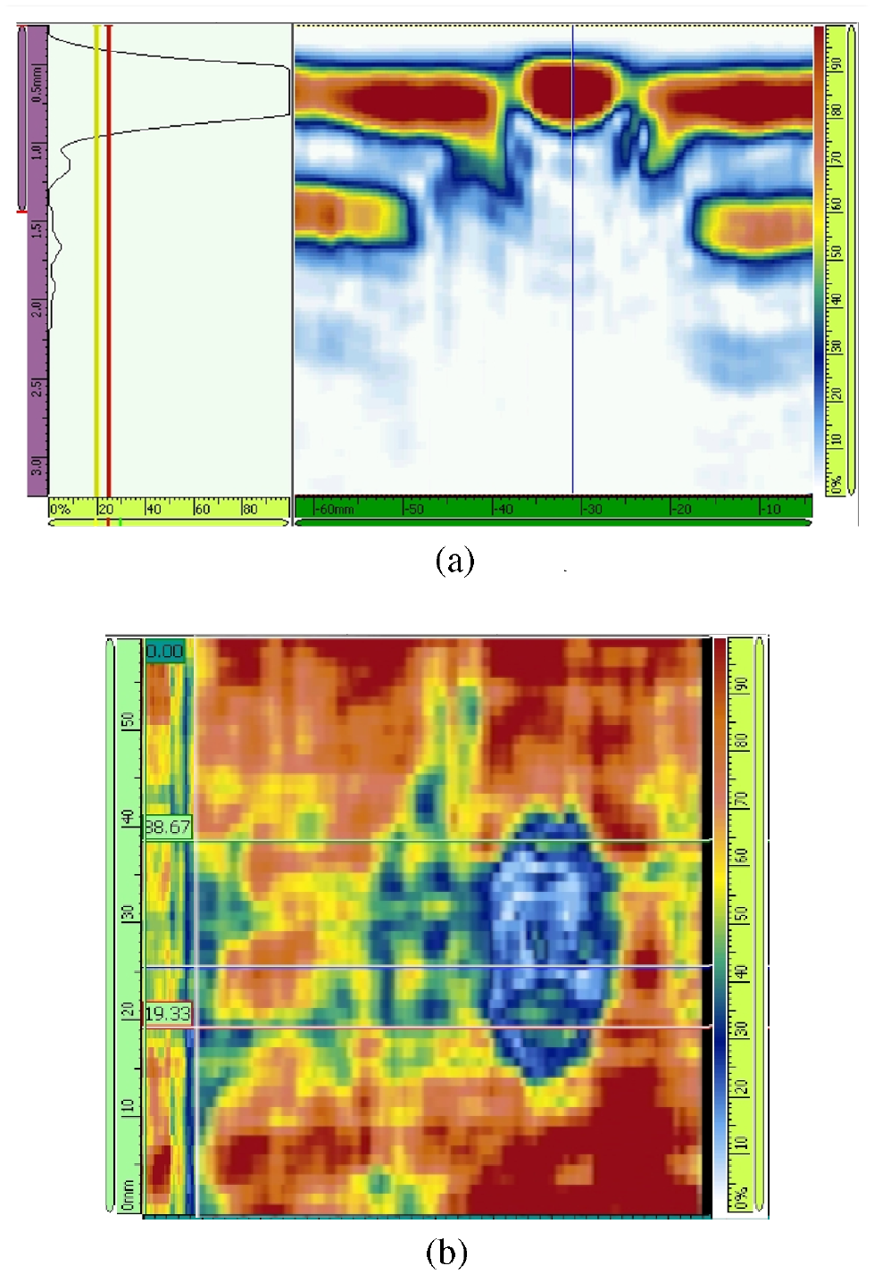
NDT results on damage location: (a) A- and B-scan and (b) C-scan.
This damaged area is then introduced in the simulation, assuming a uniform boundary reflection factor
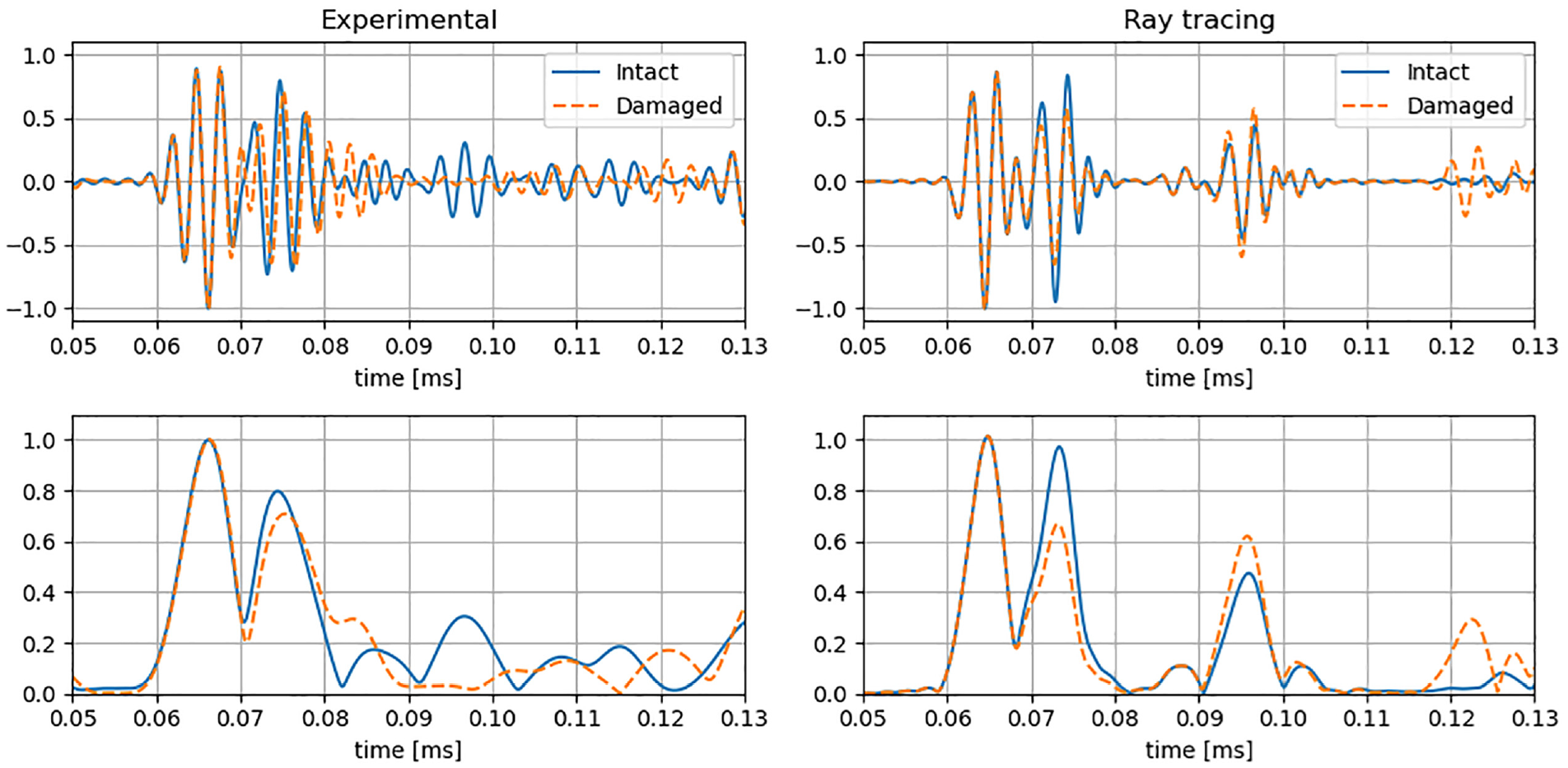
Raw signal and Hilbert transform of relevant sensor path
Results contours for the configurations evaluated on LIBIS wing prototype, at
As the damage is not directly located across the line joining sensors
Again, main differences can be explained with the same reasoning exposed in the previous sections, but additionally this case presents the complications inherent to the damage characterization. A small but appreciable frequency shift is also observed in the experimental results, which does not appear in the ray tracing simulation as the damage is still modeled as a zero width boundary.
Conclusion
The conducted tests on the metallic plate have proven instrumental in validating the proposed ray tracing methodology in a representative structure; the method demonstrates its capability to predict the guided Lamb wave propagation accurately, and as shown in the results, both initial wave packet and reflections appear with precision in arrival times and amplitude. This demonstrates and enhances the practical applicability of the methodology, and therefore, it increases the confidence when applying the validated ray tracing method to more complex composite structures.
The metallic plate study is compared with a conventional FEM dynamic explicit time integration simulation. The results shown are similar in accuracy, but computation times differ in nearly two orders of magnitude, even when using a significantly better machine to run the FEM simulation. This reinforces the adequacy of using the ray tracing method for machine learning applications, as the time to run a set of simulations required to train an artificial neural network would be significantly faster.
The boundary dissipation factor adjustment with the metallic plate study has converged to a reasonable low value and is consistent with the expected magnitude for these kinds of structures. This value is then used for the tests on the CFRP LIBIS wing lower cover demonstrator.
Results on the CFRP LIBIS wing lower cover show a significant match and similar tendencies in the presence of damage between the tests and numerical analysis. The possibility of damage could be identified, and its location and extent could be assessed by analyzing the data with cross correlation algorithms or the information could be used to feed an artificial intelligence model.
The correlation can be improved with a better characterization of the boundaries considering also the effects on frequency and propagation mode. This effect accumulates on each reflection, and the differences increase with the time of study. Exact sensor positioning, manufacturing imperfections, and other factors, discussed previously, can also alter the results, and its influence is also accumulated in time.
The results of real damage are difficult to interpret due to all the uncertainties present in this analysis; however, the methodology proposed can still present a good degree of accuracy, and some of the effects on the signal are still captured and can be observed in the presented results. Further study should be performed to improve the simulation results, that could include a more detailed characterization of the damage, by considering a nonlinear response on the resulting signal frequency.
Footnotes
Correction (February 2025):
The author affiliation of this article has been updated, since its original publication.
Declaration of conflicting interests
The author(s) declared no potential conflicts of interest with respect to the research, authorship, and/or publication of this article.
Funding
The author(s) disclosed receipt of the following financial support for the research, authorship, and/or publication of this article: This project has received funding from the national research program Retos de la Sociedad under the Project STARGATE: Desarrollo de un sistema de monitorización estructural basado en un microinterrogador y redes neuronales (reference PID2019-105293RB-C21).