
Abstract
Addressing the challenges of non-unique decomposition outcomes and prolonged decomposition durations in the fault feature adaptive extraction algorithm based on tensor decomposition, this paper presents a novel algorithm called the adaptive variable sampling tensor singular spectrum decomposition (T-SSD) algorithm. The proposed approach centers on decomposing multichannel time series with adaptive sampling frequency, leveraging tensor singular value decomposition. Initially, the embedding dimension and the number of resampling points were optimized by power spectral density analysis and adaptive sampling algorithm. Subsequently, a third-order tensor is constructed based on the principle of tensor-tensor-preserving order multiplication, combining trajectory tensor construction and embedding dimension. Finally, the signal decomposition and reconstruction of multichannel component signals are achieved through adaptive sampling, interpolation, and complementary back steps. Experimental signal analysis indicates that this algorithm can better extract fault characteristics from signals compared to common signal processing algorithms. In comparison with the traditional T-SSD algorithm, this method significantly improves decomposition efficiency, particularly for low-frequency components. It effectively tackles the efficiency challenge caused by data redundancy, enabling the organic fusion and adaptive decomposition of multichannel signals.
Keywords
Introduction
Due to the environment in which mechanical equipment works, coupled with factors such as improper human operation equipment aging and other reasons, rotating machinery inevitably experiences failures. These failures often pose significant risks to property and personnel safety during operation. Bearings are the most basic components of rotating machinery. Therefore, the fault diagnosis of bearings has always been the top priority of scientific research. Currently, the field of fault diagnosis is mainly focused in two directions: one involves establishing a kinetic model of the equipment from the perspective of dynamics to analyze and research the failure mechanism; the second involves exploring signal processing algorithms for noise cancellation and fault feature extraction from vibration signals generated during the operation of the equipment. The existing signal processing algorithms mainly include empirical modal decomposition (EMD), 1 variational modal decomposition (VMD), 2 local mean decomposition 3 and singular value decomposition (SVD). Matrix SVD is also suitable for analyzing noise-colored vibration signals. SVD is a form of principal component analysis. 4 Compared with the sine and cosine of Fourier analysis, the advantage of the SVD is that the derived components are not necessarily harmonic functions, which makes it more suitable for analyzing non-stationary time series. By using SVD to decompose a matrix, singular values that represent the most basic characteristics of the matrix are obtained. The noise-containing signal trajectory matrix can be decomposed into multiple interpretable subspace components, comprising the useful fault characteristics components and useless interference components. The singular values of the components where the noise is located are discarded and only the useful signal is reconstructed, thus obtaining the purpose of removing the noise to obtain the fault characteristic frequency. The use of the SVD method has significant advantages when dealing with noise-containing signals.5,6
Currently, numerous scholars are devoted to the research of SVD in fault diagnosis. For example, Li et al. 7 proposed a correlated SVD method for bearing fault diagnosis that combines reconstruction component determination, optimal Hankel matrix structure selection, and envelope power spectrum analysis. In Golafshan and Sanliturk, 8 an SVD and Hankel matrix-based de-noising algorithm is successfully used for ball bearing localized fault detection in both time and frequency domains. This approach helps eliminate background noise and improve the reliability of the fault detection. Qiao and Pan 9 proposed an adaptive and singular value selection method based on correlation coefficient for fault feature detection, which achieves good results in detecting weak fault signals of rolling bearings. Wang and Xin 10 proposed a weighted low-rank sparse model for bearing signal analysis that utilizes the low-rank physical structure of the periodic pulse characteristics. Zhang et al. 11 proposed a clustered low-rank method for fault diagnosis of engine bearing signals, which effectively eliminates the pathological phenomenon of overlapping of singular values and realizes the simultaneous detection of strong and weak features.
Although matrix SVD has certain advantages in dealing with noisy vibration signals, the algorithm still has certain limitations in dealing with multichannel signals. When a mechanical system fails, multiple parts and measurement points within the system may contain critical fault information. The use of multi-dimensional sensors to collect vibration signals from different locations of the system can effectively avoid the loss of local information.
Tensor as the most intuitive expression of higher-order data, not only can maintain the internal structure characteristics of the data itself, but also in the subsequent computational decomposition process closest to the essential properties of the data, so that the higher-order model will be more accurate in the data expression. 12 Vectors are first-order tensors and matrices are second-order tensors. If the signal is single-channel, the signal is usually expressed in the form of a vector and matrix, such as the time-domain waveform, spectrum, and time-frequency diagram of the signal. According to the mathematical significance of tensors, tensor decomposition is expected to overcome the limitations of matrix SVD when processing multichannel signals. Currently, a growing number of scholars have dedicated their efforts to the study of tensor decomposition, and it has been utilized in various fields.13–19 The mainstream tensor decomposition methods in use are Canonical Polyadic (CP) decomposition, 20 Tucker decomposition, 21 and higher-order SVD (HOSVD).22–24 These methods are continually being optimized and refined. Since signals inevitably appear to be missing in the process of storing or transmitting, Zhou et al. 25 put forward an iterative HOSVD image missing data recovery method for efficient recovery of missing data in images. This method makes full use of the multiple constraints within the image and between the image and the image, and greatly improves the recovery accuracy. Combining the advantages of HOSVD and quaternion, Miao et al. 26 proposed a multi-focus color image fusion method and a color image denoising method. Karim et al. 27 proposed a new variant of the Levenberg-Marquardt algorithm used for Tensor CP decomposition with an emphasis on image compression and reconstruction. Li et al. 28 presented joint adaptive threshold HOSVD and the rearrangement of pixels in tensors method for image denoising, which exploits more prior knowledge to characterize the image features. Mao et al. 29 proposed a new self-supervised deep tensor domain-adversarial anomaly detection model, named Tensor-DAAD. Tensor-DAAD can find early fault occurrence in an earlier location with a much lower false alarm rate. The SVD of matrices has been extended to higher order in many ways, 30 but since the essence of the HOSVD algorithm is still to utilize the idea of matrices to deal with signals, there are problems of non-pseudo-diagonal core tensors and non-unique decomposition results in dealing with multichannel signals. To solve the above problems, Kilmer et al. 31 defined a new tensor multiplication rule and the corresponding T-SVD. Based on the principle of tensor-preserving multiplication proposed by Kilmer, Huang and Cui 32 developed a tensor singular spectrum decomposition (T-SSD) algorithm based on T-SVD, which can better extract the weak fault quantization features hidden in the original multichannel signal. Xu et al. 33 used the tensor core norm to represent the low-rank structural information of tensor data and developed a new low-rank tensor-based semi-supervised classifier, which can perform semi-supervised analysis of large multi-sensor signals when the number of labels is limited case, this method achieves high-accuracy fault classification. However, since tensors are usually used as high-order expressions, the length of data involved in T-SSD calculations is very sensitive to its computational efficiency, therefore, how to compress the computing time of T-SSD on the premise of retaining the advantage of tensor decomposition to extract weak fault features is a very challenging topic.
The core contribution of this paper is to propose the adaptive variable sampling T-SSD algorithm, which addresses the inefficiencies found in the traditional T-SSD method. To implement this innovation, the algorithm first evaluates the features of signals within the decomposed bandwidth, which informs the subsequent construction of a third-order tensor tailored to the specific characteristics of the signal. The signals are then resampled using an appropriate sampling frequency, and a tensor with suitable dimensions is built for decomposition. Subsequently, the component signals obtained from the iteration process are thoroughly assessed. The resampled signal components are reintegrated into the original signal’s components of equal length through interpolation. This step ensures that subsequent iterations are not affected by differences in array length. This approach fundamentally solves the problem of low computational efficiency (or even freezing) in traditional T-SSD, especially concerning the decomposition of low-frequency signal components.
The paper’s structure is outlined as follows: the section “Signal processing based on T-SVD” introduces tensor multiplication, the rule of T-SVD, and the traditional T-SSD. Section “The proposed method” presents a novel adaptive variable sampling T-SSD algorithm. This algorithm is developed based on T-SSD, adaptive sampling and the principles of interpolation complementation. It realizes resampling different data points when decomposing different frequency bands. Following components acquisition, the interpolation complementary back algorithm is executed. Section “Verification using experimental signals” the advantages and accuracy of the proposed method are verified by the experimental signal processing results. Section “Conclusion” provides a conclusion summarizing the key findings.
Signal processing based on T-SVD
Definition of notation and new tensor multiplication
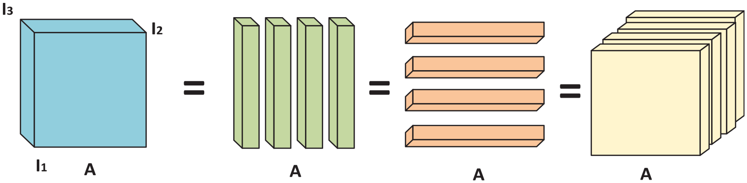
Three different mode slices of a third-order tensor.
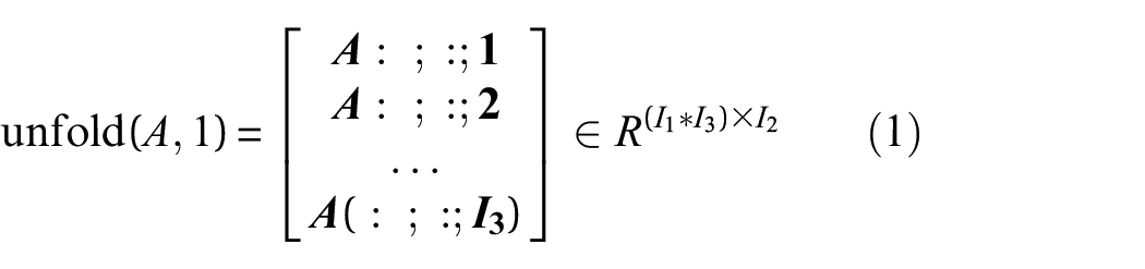
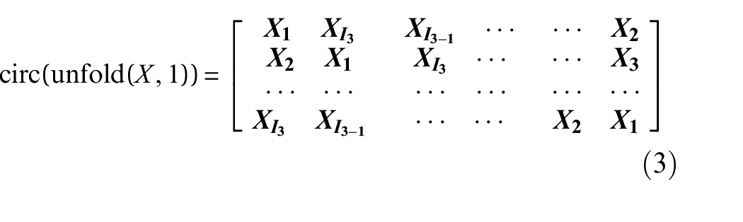
In tensor analysis, unfold and fold are frequently used operations of a tensor, where a third-order tensor is unfolded to be analyzed in a second-order tensor, and the second-order tensor is collapsed back to a third-order tensor after analysis to observe its features, for example, the positive expansion of the tensor
The second parameter
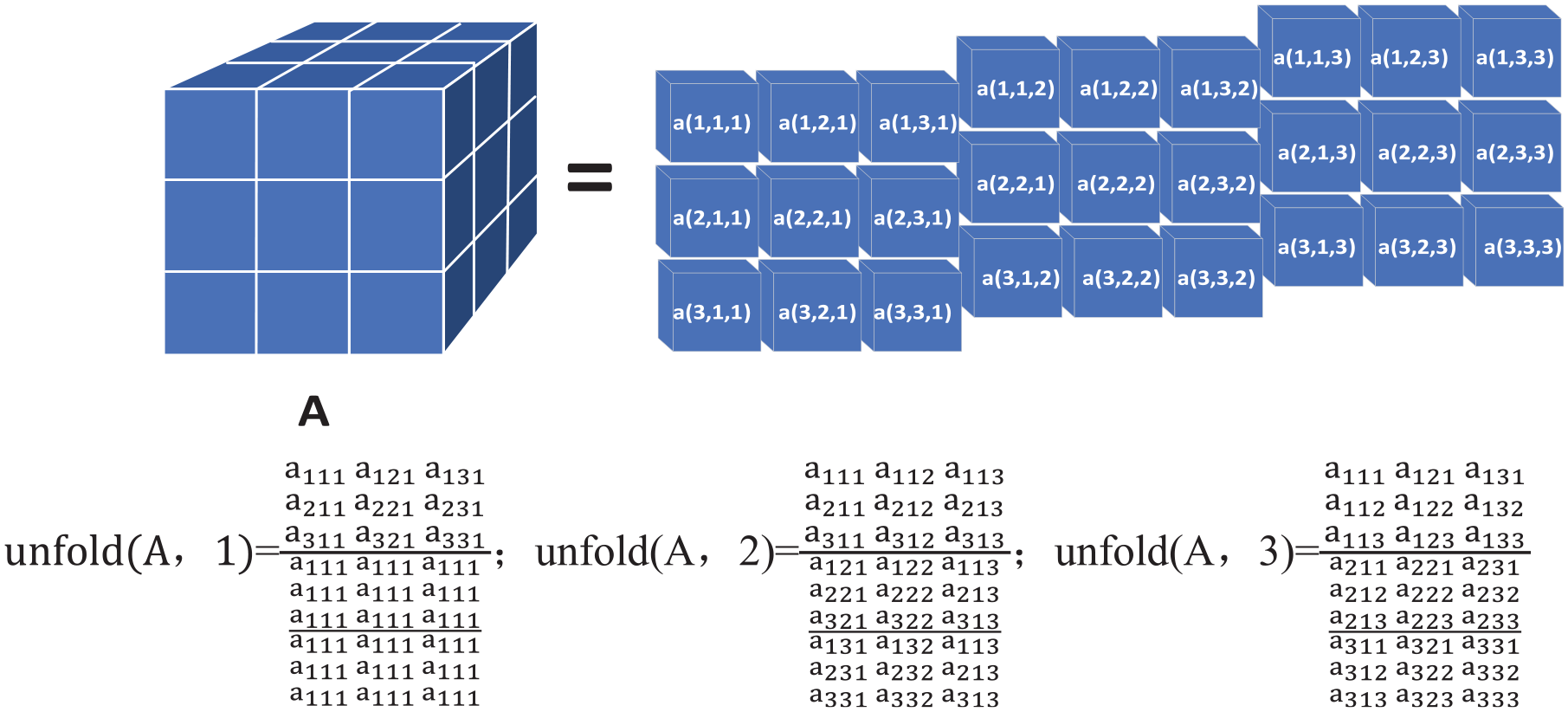
Different mode expansions of a third-order tensor.
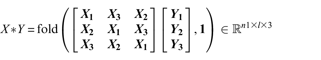
The multiplication of the different expansion modes of the tensor and the matrix is defined as the n-mode product. The n-mode product does not apply to the multiplication of two third-order tensors. Thus, a new multiplication rule of the tensor is proposed and its properties are described below.

For example,
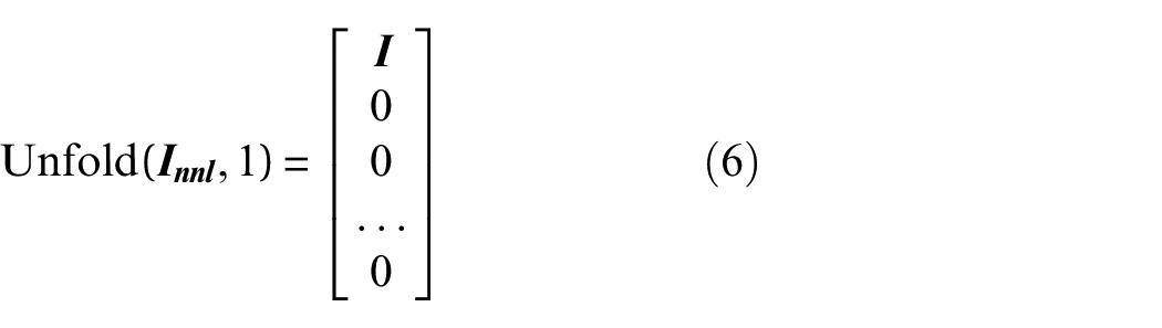
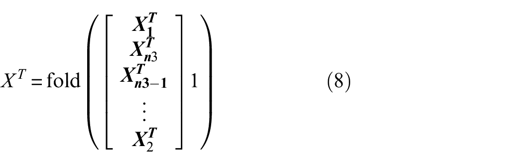
The unfold and fold in Equation (2) denote the tensor unfolding and folding operations respectively, they are inverse operations to each other;
From Kilmer et al.,
31
it is known that the discrete Fourier transform (DFT) can diagonalize cyclic matrices, and similarly, block-cyclic matrices can be diagonalized by DFT. Assuming that the size of the tensor
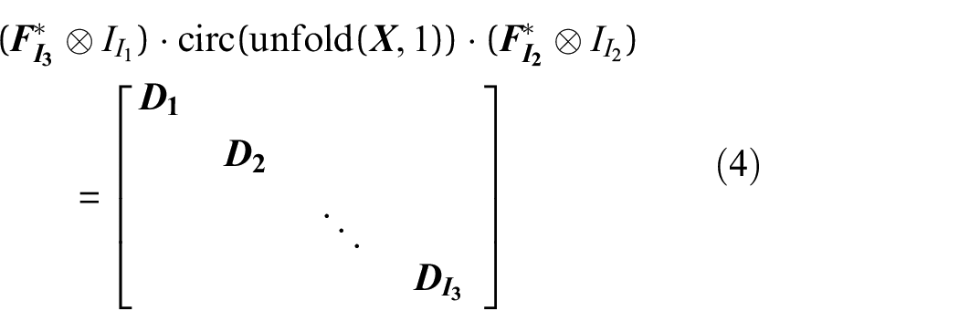
where “⊗” refers to the Kronecker product,


That is,
Transposition of a tensor
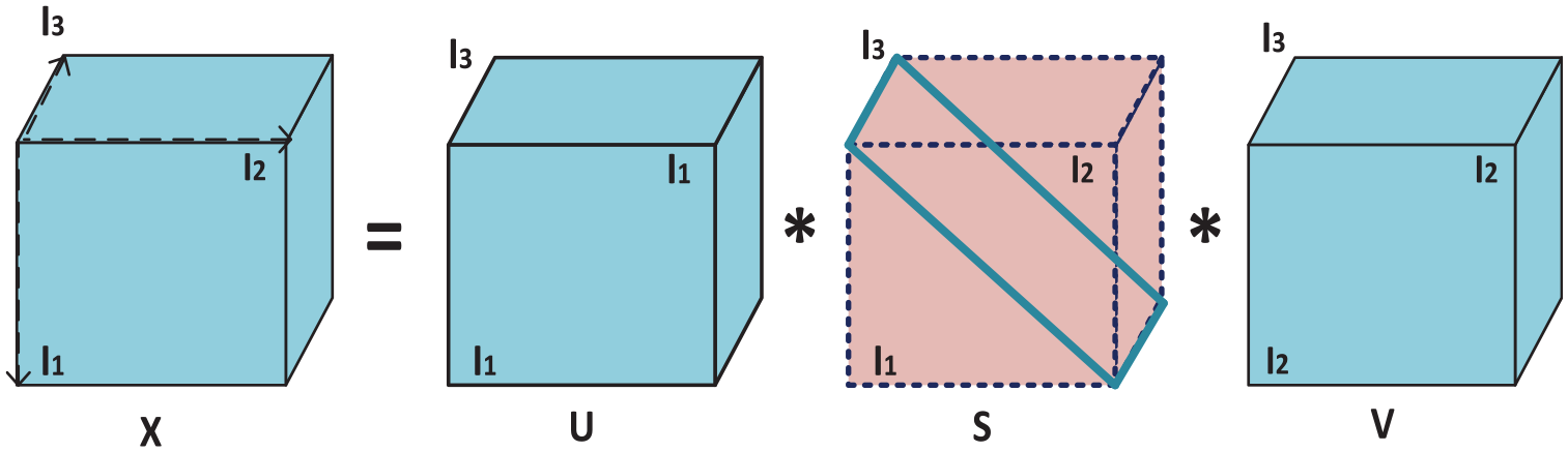
Tensor SVD
If

where
Schematic diagram of third-order tensor T-SVD.
Table 1 shows the steps of T-SVD, and Figure 3 shows the corresponding decomposition mode.
T-SVD methods.
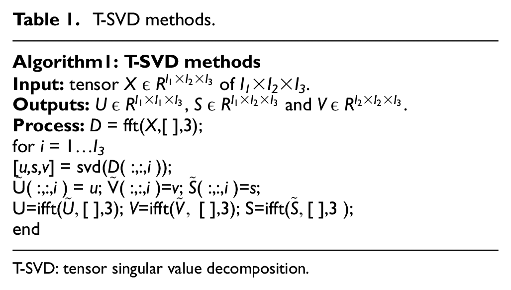
T-SVD: tensor singular value decomposition.
Proof: SVD is applied to each matrix
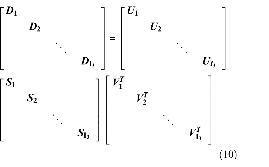
Simultaneous left multiplication by
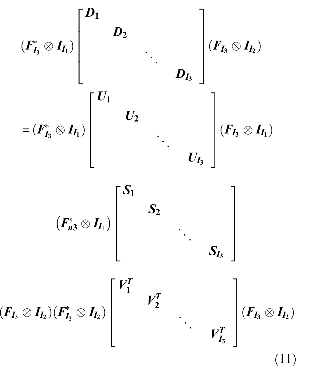
It follows from Equations (4) and (11):
i.e.:
Construction of tensor models
A single-channel vibration signal acquired from a single sensor is represented as a vector. Therefore, to capture multichannel signals, it is essential to employ multiple sensors. Subsequently, these multichannel signals are combined and organized into a higher-order tensor, facilitating the representation of signals in higher dimensions. The T-SSD adopts the method of constructing the trajectory matrix from the matrix singular spectrum decomposition in Bonizzi et al.
34
and extends it to higher order. Taking two-channel signals as an example, assuming that the one-dimensional signals obtained by the two sensors are discrete time series, denoted as
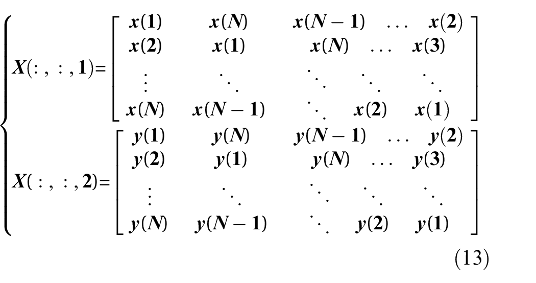
The number of frontal slices coincides with the number of sensors. The expression of the Equation (13) is for the relation when
A simulated signal is formed by integrating a harmonic signal (component 1) and an impulse signal (component 2).

where
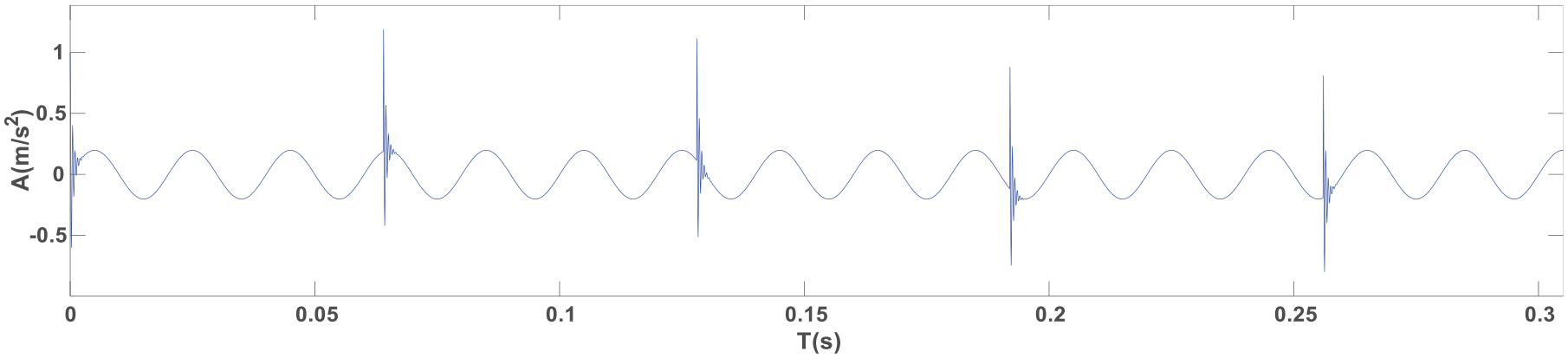
Time-domain diagram of simulated signals.
The third-order tensor is constructed from the simulated signal, in which the
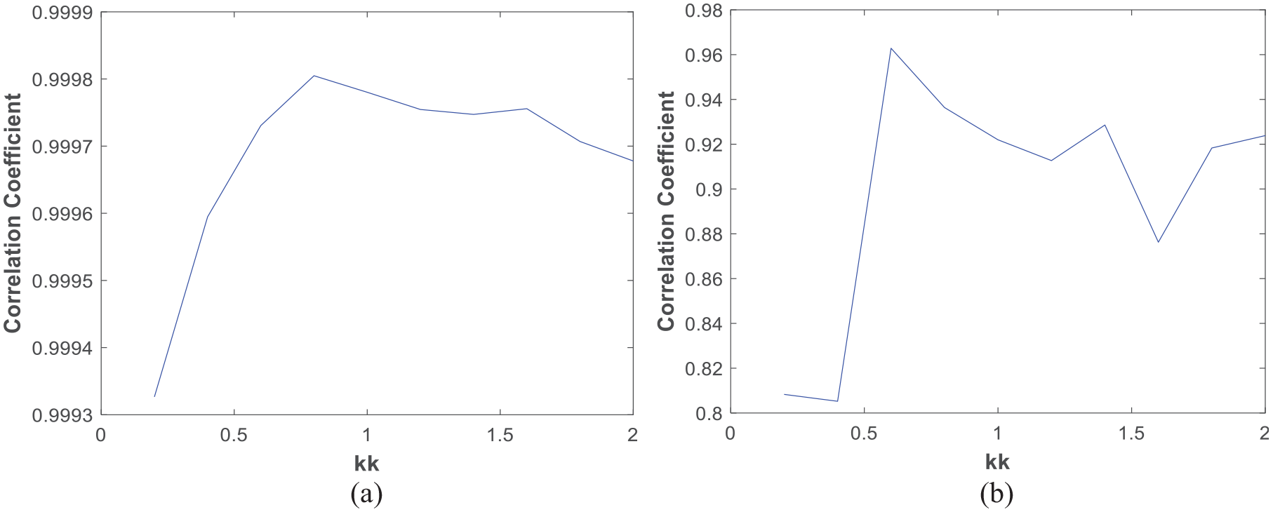
The components obtained by the proposed method are compared with those of the original signal. Correlation coefficients between the components obtained by the proposed method and those of the original signal are calculated for different
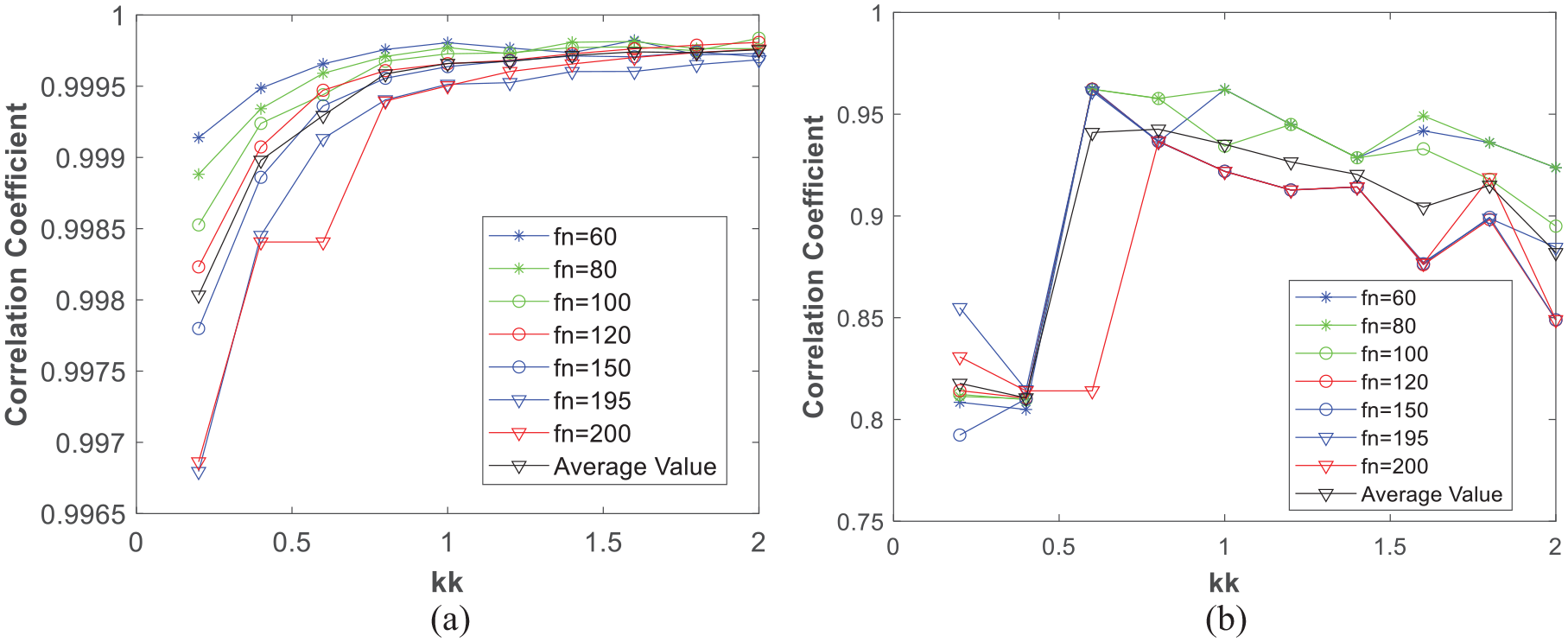
Correlation coefficient of decomposed components and the original signal at different
As can be seen in Figure 5, the correlation coefficients are bigger when the
Correlation coefficients of the components obtained by the adaptive variable sampling T-SSD algorithm and original signal’s components: (a) Component 1 and (b) Component 2.
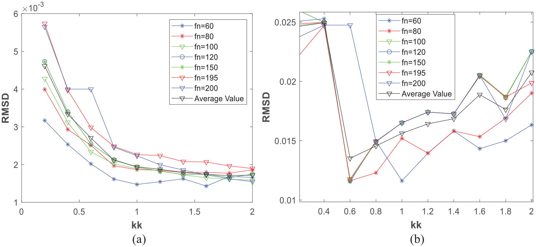
RMSE of the components obtained by the adaptive variable sampling T-SSD algorithm and the original signal’s components: (a) Component 1 and (b) Component 2.
From Figures 6 and 7, it can be obtained that the two components exhibit higher correlation coefficients and lower RMSE when kk ranges from 0.8 to 1.2. Therefore, kk is most effective within this range. In this study, kk is set to 1.2 in the algorithm.
Adaptive selection of multichannel component signals
After building the third-order tensor
In determining the current iteration range, the matrix singular spectrum method proposed in Kilmer et al.
31
is used, that is, an iterative method is used to extract the component signals
where,
where,
Steps of signal decomposition based on T-SVD.
The proposed method
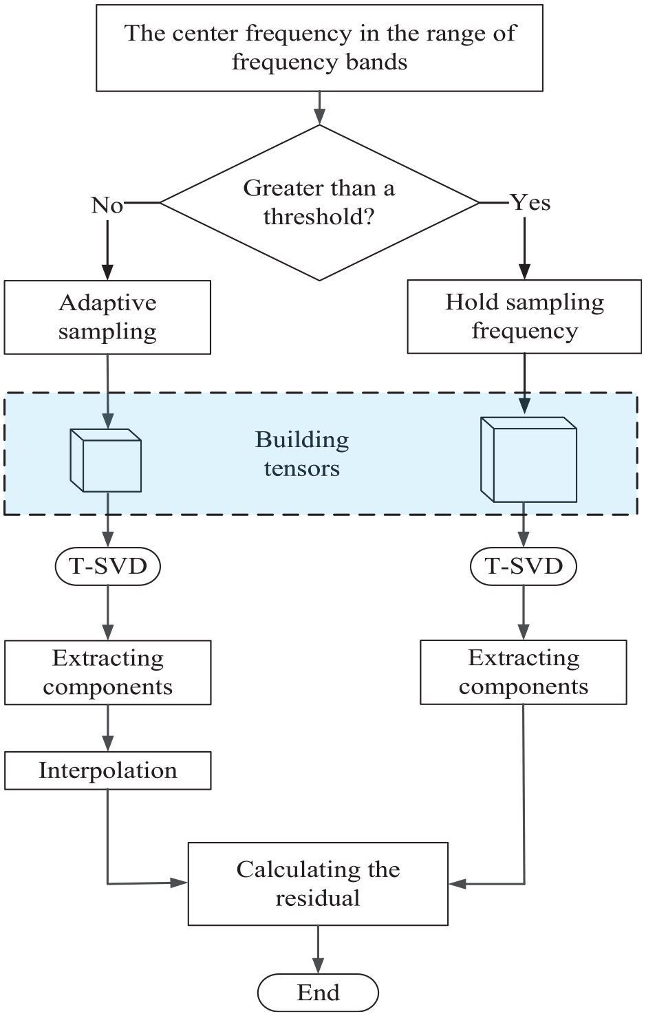
The algorithm described in Figure 8 operates with the frequency of the extracted components selected according to the PSD. The algorithm maintains fixed sampling frequency and sampling point numbers. If a higher sampling frequency persists during the extraction of components with lower frequencies, it will generate redundant data, thus inflating the dimensions for subsequent tensor construction. As a result, the decomposition time is prolonged and the decomposition efficiency is reduced. To solve the above deficiencies, this study proposes the adaptive variable sampling T-SSD algorithm. The optimal parameters are selected according to the center frequency of the selected component range to perform adaptive sampling and interpolation complementing, which solves the problem of low efficiency and even stuck caused by tensor data redundancy.
Adaptive down sampling
Based on the results of the comparison between the center frequency of the band range delineated in the current iteration and the set threshold, it is determined whether adaptive sampling is used in the current decomposition process, where the number of sampling points changes with the change of the center frequency of the component, and the number of sampling points
where

The signal component length
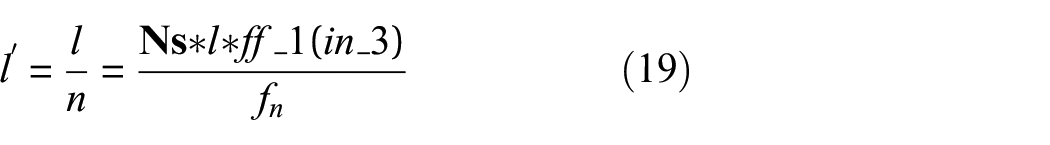
where
A simulated signal
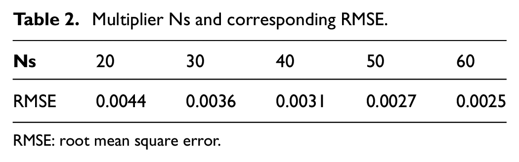
Multiplier
RMSE: root mean square error.
Based on the values of
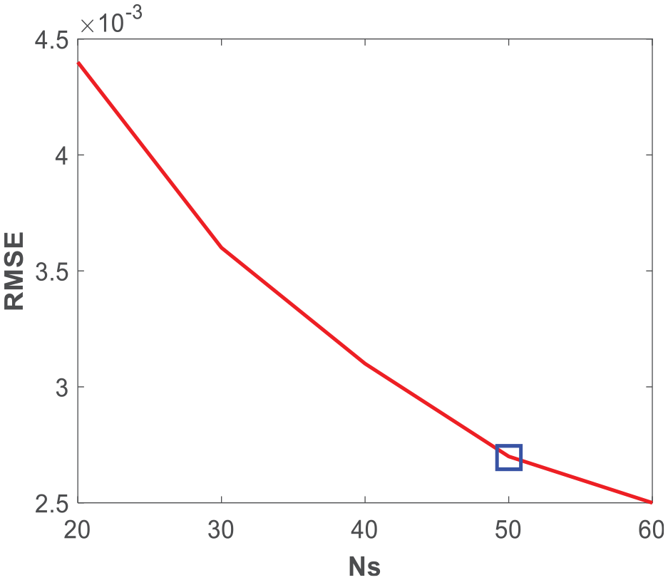
The sampling frequencies are different multiples
The threshold

where,
When the value of
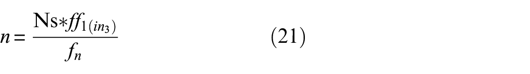
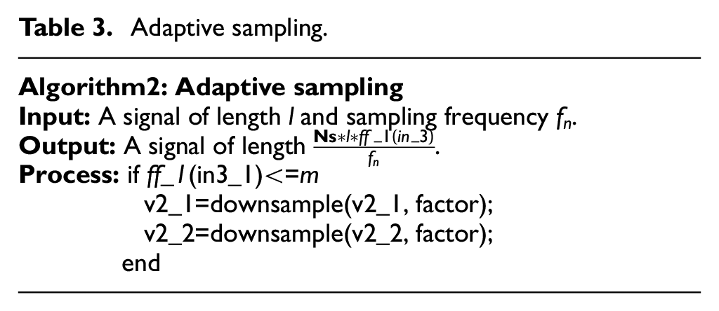
Table 3 gives the steps of adaptive sampling.
Adaptive sampling.
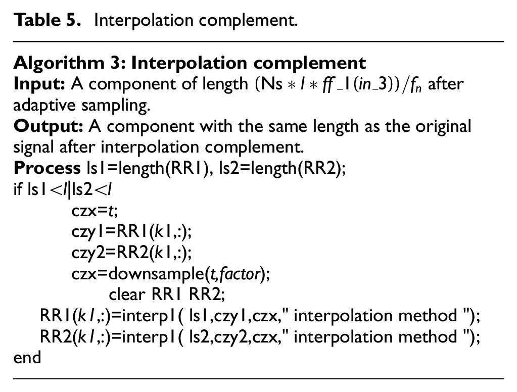
Interpolation complement
After adaptive sampling, the iterative decomposition often yields component signals length of shorter length compared to the original signal. This discrepancy can impact the calculation of the residual (residual signal = original signal – iterative component). Hence, when the decomposition and extraction of component signals in adaptive sampling, it becomes necessary to complementarily interpolate back to the length of the original signal before proceeding with subsequent iterative loops. The interpolation complement algorithm in this paper needs to first judge whether the length of the obtained component matches that of the original signal. This assessment helps determine if the current component has undergone adaptive sampling. Subsequently, the algorithm decides whether the current component needs interpolation complementation. In MATLAB, the main interpolation methods for one-dimensional arrays include
RMSE of interpolation methods and corresponding time consuming.
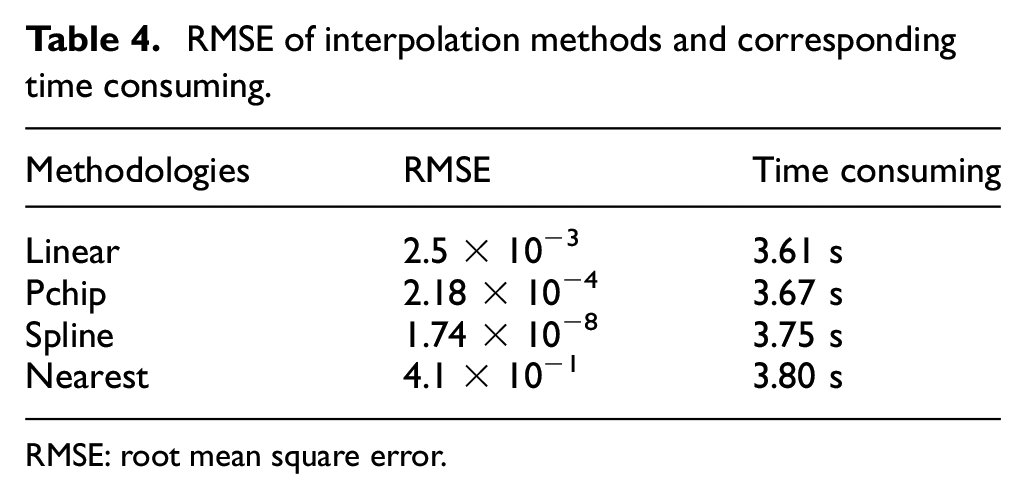
RMSE: root mean square error.
Interpolation complement.
Main steps of the adaptive sampling algorithm.
Adaptive variable sampling T-SSD algorithm
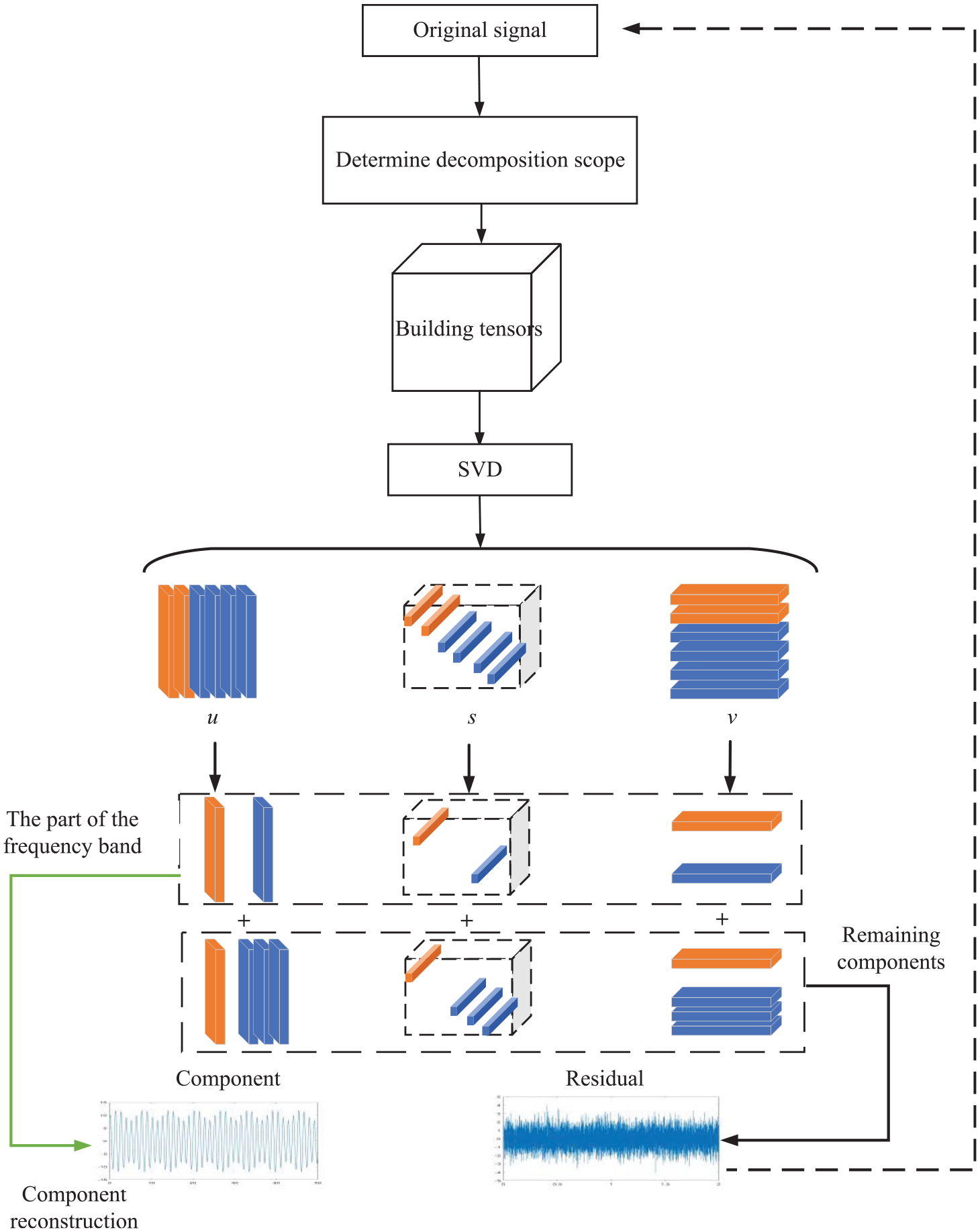
This section proposes an adaptive variable sampling T-SSD algorithm combining adaptive sampling and interpolated supplementary algorithm. The flowchart of the proposed method is shown in Figure 11, and its main steps are as follows.
Step 1: Determine the range of signals to be decomposed based on the PSD.
Step 2: According to the signal characteristics in the current iteration range, the adaptive downsampling step is carried out to reduce unnecessary redundant data.
Step 3: The higher-order tensors with appropriate dimension size are established and T-SVD decomposition is carried out. Select the corresponding singular values in the range to reconstruct the signal and get the component signals.
Step 4: By comparing the component length obtained by decomposition with the length of the original signal, the implementation of the interpolated supplementary algorithm is selected adaptively to ensure the smooth progress of the subsequent iteration.
Step 5: The decomposition reaches the termination condition, obtains a series of components, and the decomposition is complete.
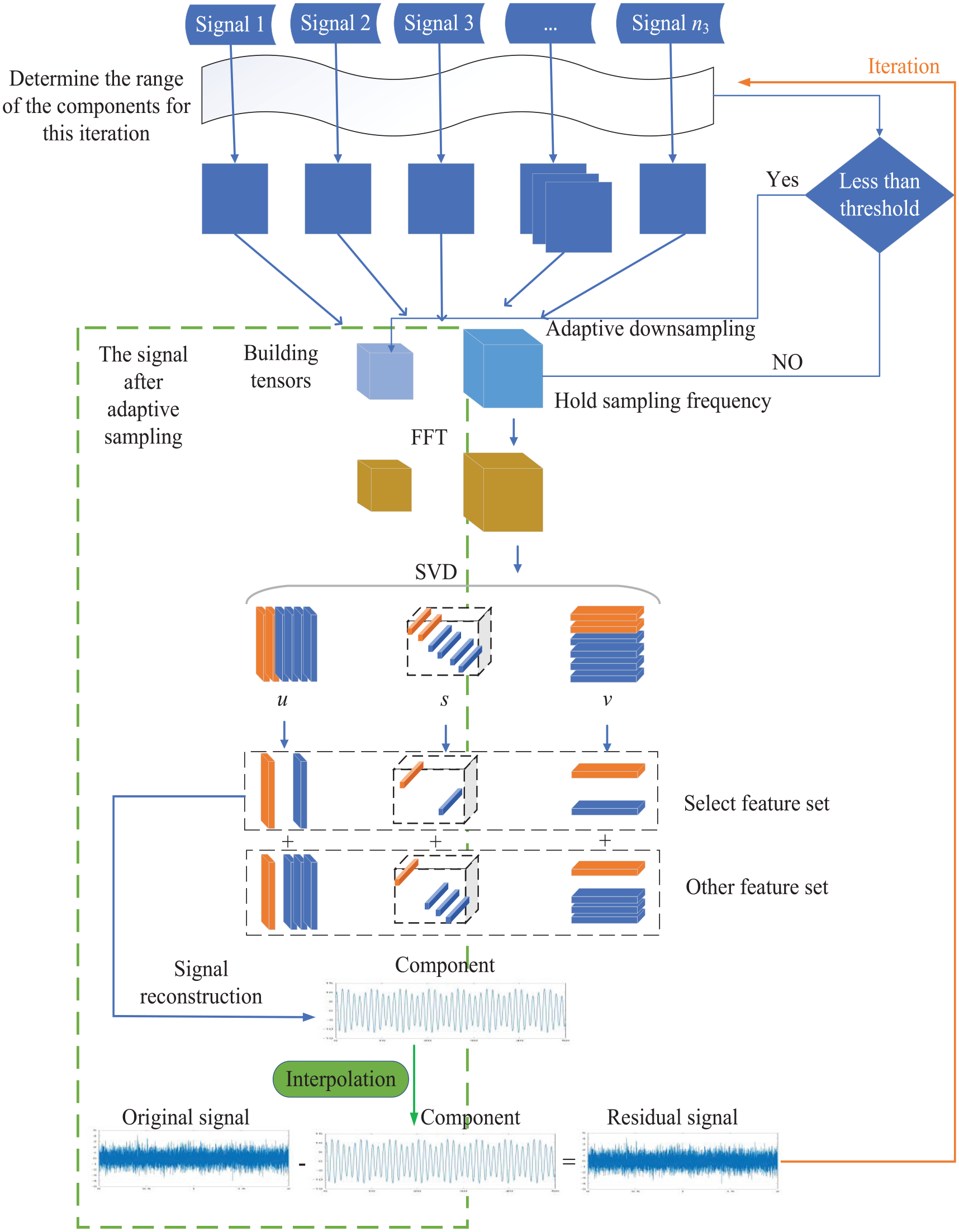
Flowchart of the adaptive variable sampling T-SSD algorithm.
Verification using experimental signals
To verify the validity of the adaptive variable sampling T-SSD algorithm, experimental data from a gearbox are used. A fault is located on a bearing on one of the gearbox’s three output shafts. Six acceleration sensors are installed on the experimental gearbox, and the relative positions of these sensors are shown in Figure 12.
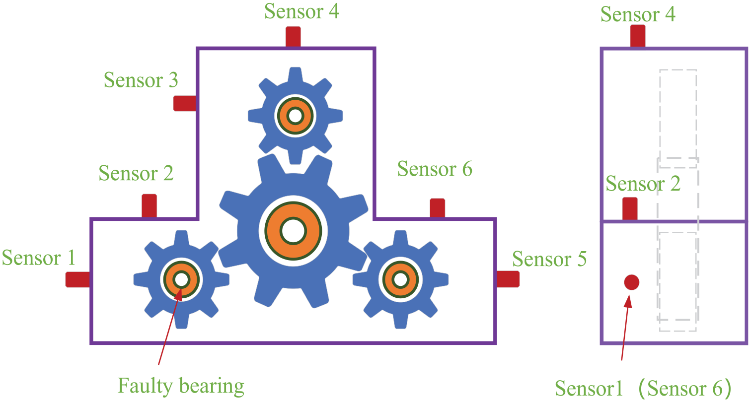
The relative position of the sensor on the experimental gearbox.
Figure 13 shows the faulty bearing with a 1 mm hole machined on the surface of the outer ring of the bearing using electrical impulses to simulate the point of failure.
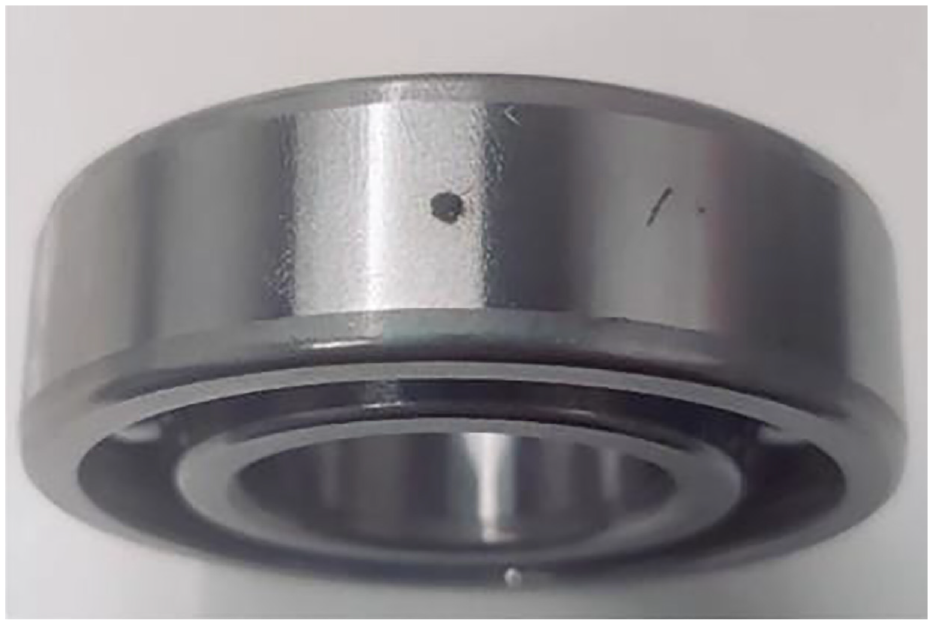
Bearing with outer ring failure.
Case 1
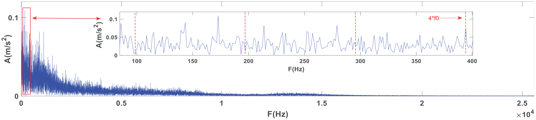
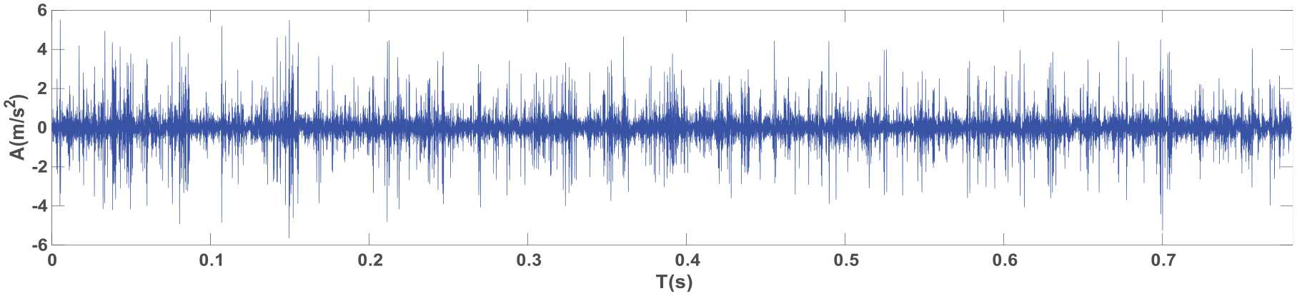
The following analysis of the experimental signal is conducted to evaluate the performance of the proposed method of this paper in extracting the fault characteristic frequency, the gearbox speed is set to 1683 rpm. The location of the faulty bearing is shown in Figure 12. Vibration acceleration sensor 1 and sensor 2, corresponding to the horizontal and vertical directions of the bearing respectively, are used with a sampling frequency of
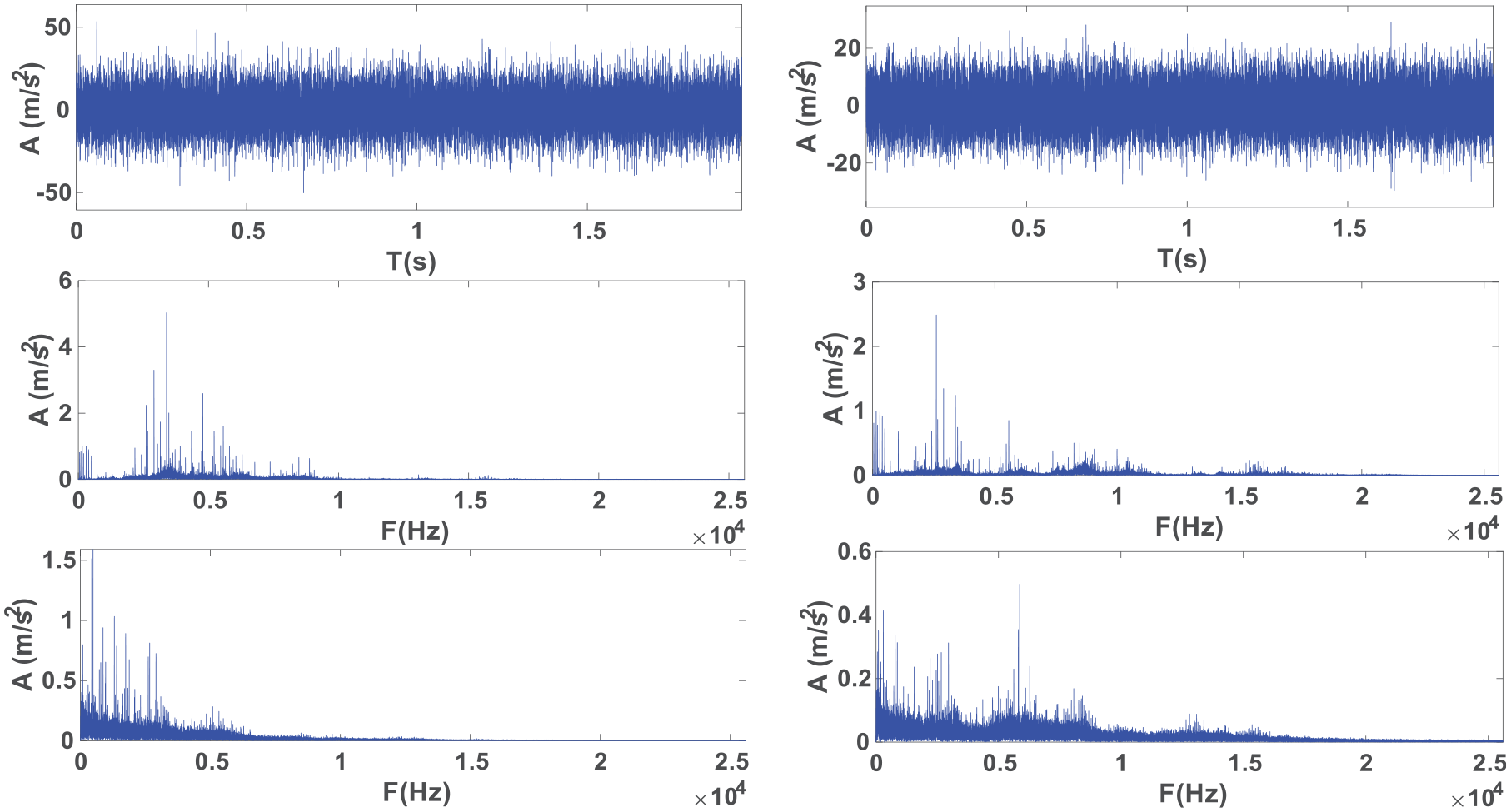
Time-domain waveform and frequency and envelope spectra of the experimental signal.
The experimental signals are iteratively decomposed by both the traditional T-SSD and the adaptive variable sampling T-SSD algorithm to obtain the component signals, as shown in Figure 15. It can be seen from Figure 15 that the fault characteristic frequency and its harmonics can be found in component 2. This indicates that the proposed method has the same feature extraction capabilities as the traditional T-SSD. However, in terms of decomposition efficiency, the traditional T-SSD algorithm requires 842.46 s, while the method proposed in this paper takes only 171.05 s, achieving an efficiency improvement of nearly five times over the traditional T-SSD.
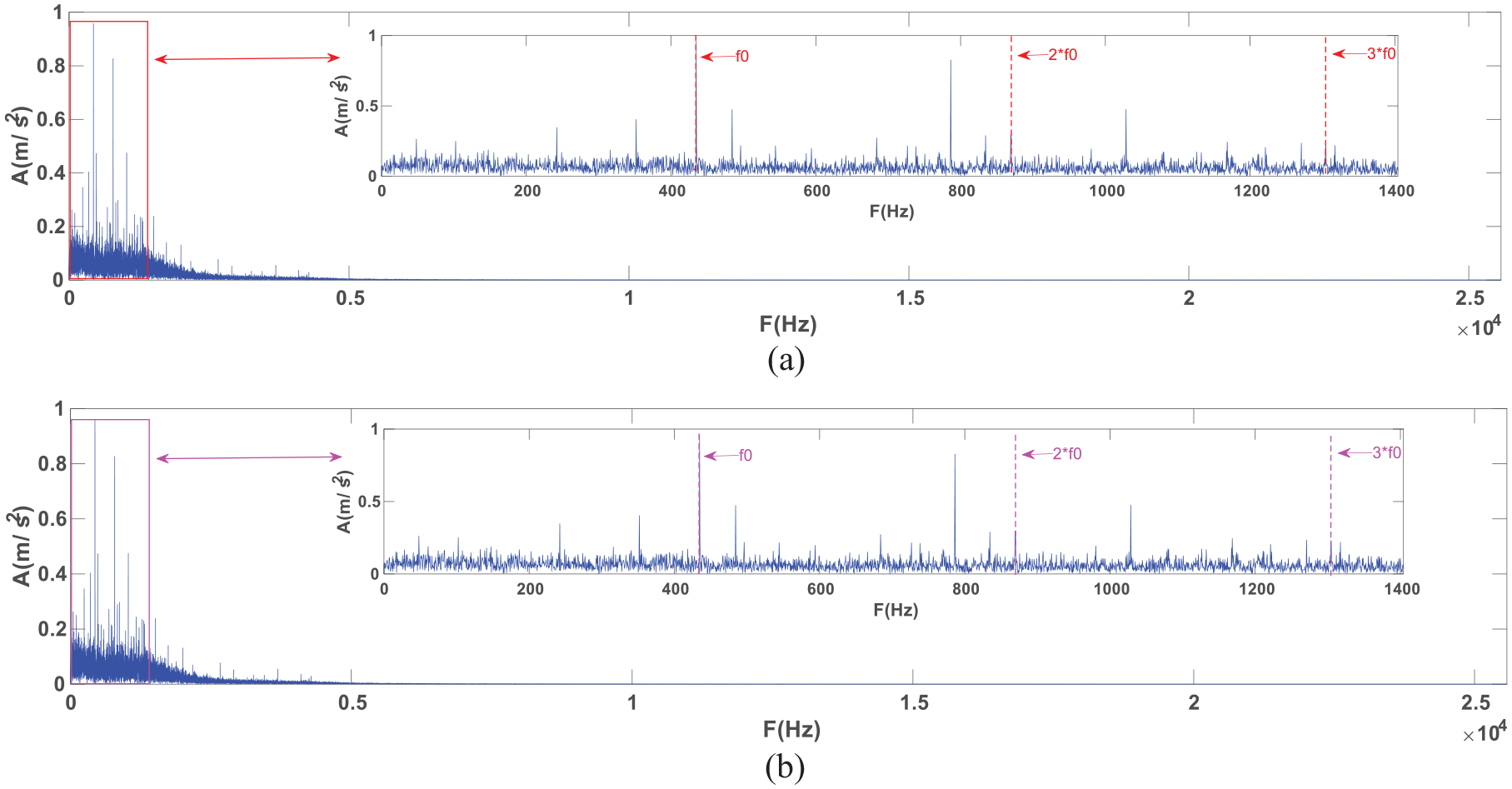
The components containing fault characteristic frequency of two algorithms: (a) Component 2 envelope spectrum obtained by traditional T-SSD and (b) Component 2 envelope spectrum obtained of adaptive variable sampling T-SSD algorithm.
Case 2
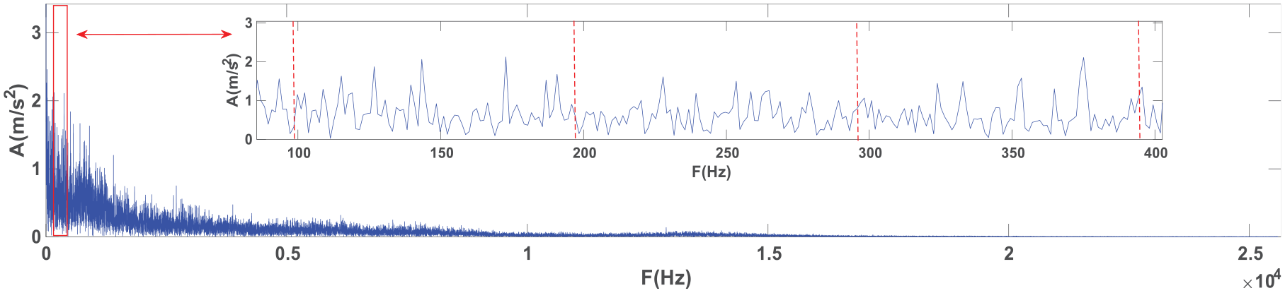
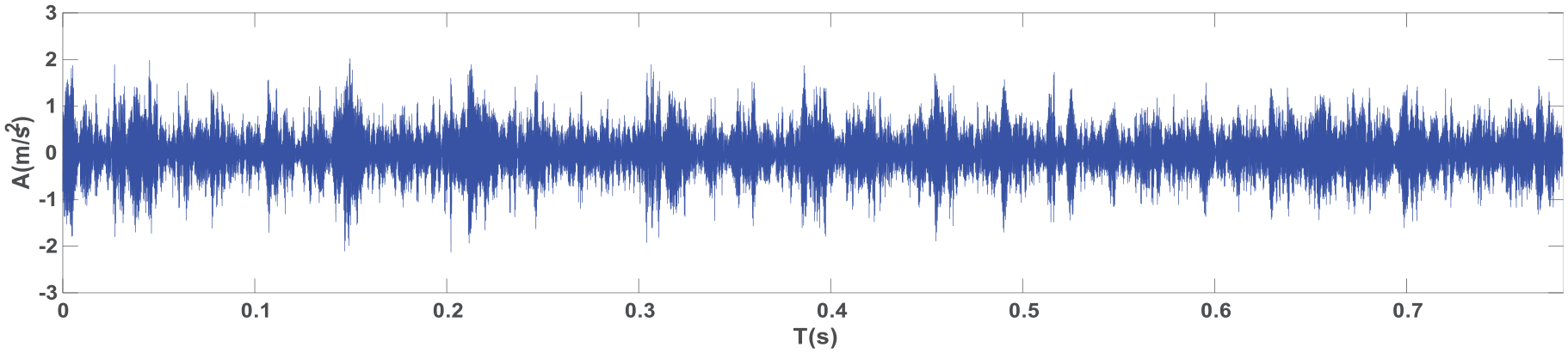
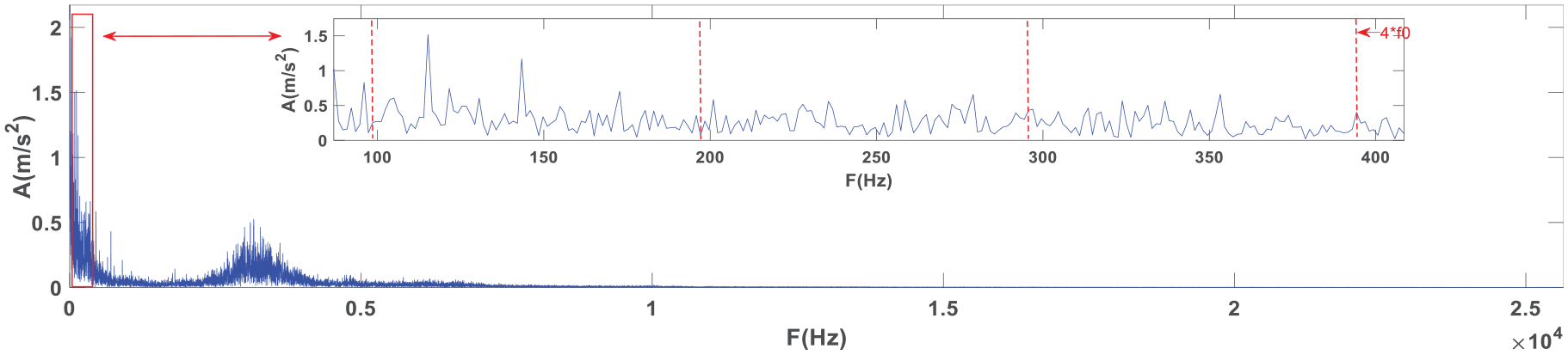
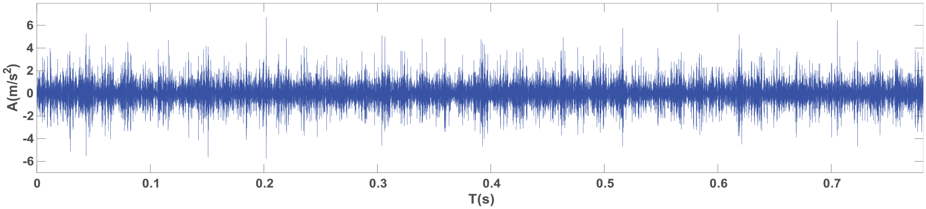
New fault vibration signals at a speed of 400 rpm are then collected from the experimental gearbox. The time-domain waveform and envelope spectrum of the experimental signal are shown in Figures 16 and 17. At this speed, the fault characteristic frequency is 98.56 Hz. Since the proposed method is a type of signal processing, in order to demonstrate its ability to explore weak fault characteristic frequency in signals, it is compared with traditional signal processing methods (EMD, VMD) using the same set of signals. EMD 35 is firstly used to decompose the vibration signal into multiple intrinsic mode functions (IMFs), and the components strongly correlated with the original signal are selected to reconstruct the signal. The time-domain diagram and envelope diagram of the reconstructed signal are shown in Figures 18 and 19.
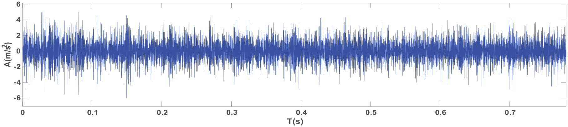
Time-domain waveform of experimental signal.
Envelope spectrum of experimental signal.
Time-domain waveform after EMD and reconstruction.
Envelope spectrum after EMD and reconstruction.
In the VMD 2 algorithm, the number of decomposition levels k, and regularization parameter α greatly influence the decomposition results. Thus, the whale optimization algorithm is used to optimize the parameters k to obtain the optimal decomposition effect. The result shows that when k is 7 and α is 2000, the result of VMD is the optimal solution. The IMFs whose kurtosis value is greater than four obtained by VMD of the original signal are reconstructed. The time-domain waveform and envelope spectrum of the reconstructed signal are shown in Figures 20 and 21.
Signal time-domain waveform after VMD and reconstruction.
Signal envelope spectrum after VMD and reconstruction.
It is evident from Figures 18 to 21 that when EMD and VMD algorithms are used to process the early fault vibration signals, the fault characteristic frequency is drowned by overwhelmed by the interference components.
Finally, the adaptive variable sampling T-SSD algorithm is used to process the same signals, and the results are shown in Figures 22 and 23. Component 2 extracted by the adaptive variable sampling T-SSD algorithm contains the fault characteristic frequency and its harmonics, which are relatively more obvious. This indicates that the adaptive variable sampling T-SSD algorithm is more effective at extracting early faults than the EMD and VMD algorithms.
Time-domain waveform of component 2 obtained after decomposition by adaptive variable sampling T-SSD algorithm
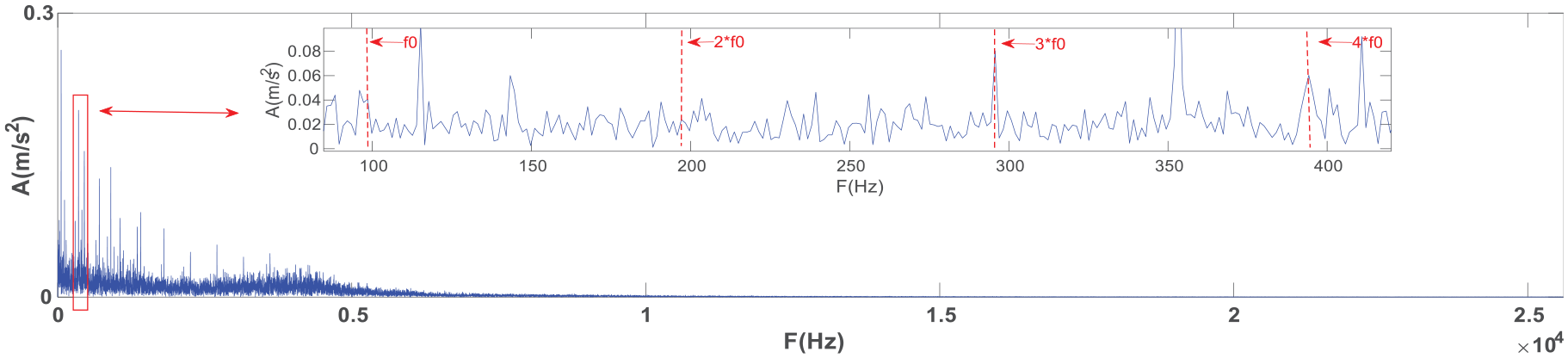
Envelope spectrum of component 2 obtained after decomposition by adaptive variable sampling T-SSD algorithm.
Efficiency analysis
The above findings underscore the significant enhancement in decomposition effect and efficiency achieved by the method proposed in this paper. To fully prove the superiority of the proposed method in terms of efficiency, three sets of vibration signals were processed using the proposed method and traditional T-SSD. The time consuming of the two decomposition algorithms and the improved efficiency of the adaptive variable sampling T-SSD algorithm are shown in Table 6. The formula used to calculate the efficiency improvement is: Efficiency improvement (%) = 100 × (time of traditional T-SSD − time of proposed method)/time of traditional T-SSD. It can be seen from Table 6 that when decomposing the same data, the adaptive variable sampling T-SSD algorithm has a faster decomposition speed. The decomposition efficiency was improved by 78%, 85.8%, and 95.7%, with an average improvement of 86%.
Comparison of time consumption of traditional T-SSD and the proposed method.
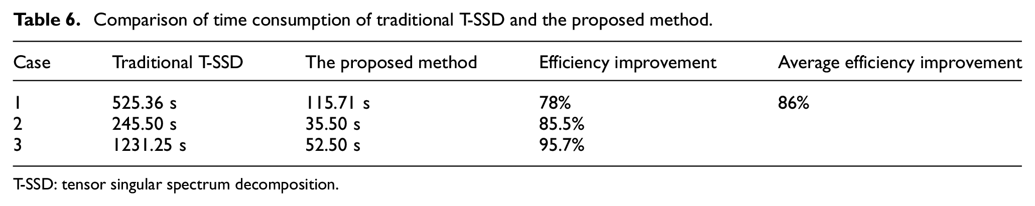
T-SSD: tensor singular spectrum decomposition.
Error analysis
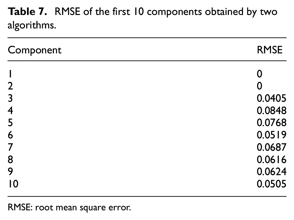
As can be seen from the section “efficiency analysis,” the proposed method in this paper has obvious advantages in decomposition efficiency. To further assess the accuracy of decomposition results, the RMSE values between components obtained from the traditional T-SSD algorithm and the adaptive variable sampling T-SSD algorithm are analyzed using the same data. These RMSE values of the first 10 components from the traditional T-SSD algorithm and the adaptive variable sampling T-SSD algorithm are presented in Table 7. From the results shown in Table 7, it is evident that the RMSEs of the first 10 components are very small, which proves the accuracy of the adaptive variable sampling T-SSD algorithm.
RMSE of the first 10 components obtained by two algorithms.
RMSE: root mean square error.
Conclusion
An adaptive variable sampling T-SSD algorithm was proposed in this paper to effectively tackle the problem of low decomposition efficiency and potential stagnation caused by data redundancy during signal processing in traditional T-SSD. Several conclusions can be drawn as follows.
The analysis results of experimental data demonstrate that the proposed adaptive variable sampling T-SSD algorithm can greatly improve signal decomposition efficiency. Specifically, when applied to the same set of experimental signals, the proposed algorithm enhances the signal decomposition efficiency by an average of 86% relative to the traditional T-SSD algorithm.
The analysis results of experimental data demonstrate that the proposed algorithm excels at extracting fault features. When analyzing early fault signals from bearings, the fault characteristic frequency and its harmonics can be clearly seen in the component envelope spectrum obtained by the adaptive variable sampling T-SSD algorithm. Furthermore, comparison analysis with traditional signal processing algorithms. (EMD, VMD) confirms that the proposed method provides superior performance in extracting weak fault features.
Footnotes
Appendix
Declaration of conflicting interests
The author(s) declared no potential conflicts of interest with respect to the research, authorship, and/or publication of this article.
Funding
The author(s) disclosed receipt of the following financial support for the research, authorship, and/or publication of this article: This work is supported by the National Natural Science Foundation of China under Grant Nos. 52105109, 52305115, and 52161135101. Natural Science Foundation of Inner Mongolia No. 2023QN05031, and the China Postdoctoral Science Foundation No. 2023M741938.