
Abstract
Harmonic magnetic field focus detection technology has been utilized for in-service pipeline defect detection due to its advantage in providing high-sensitivity and noncontact detection. However, this technology encounters interference from background signals and noise during high lift-off detection, which limits the accuracy of defect signal extraction. To quickly and robustly identify pipe defects, this work discloses a novel defect signal extraction method for multiple-harmonic magnetic field detection technology. The proposed method is insensitive to noise interference, effectively extracting defect signals even under high-intensity noise conditions. A pipe defect model based on magnetic dipole moments is established for simulation analysis, and a pipeline test platform is built for experimental validation. The results demonstrate that the proposed method can identify defects from signals with a low signal-to-noise ratio of 5.7 dB and locate pipes, welds, and defects with high resolution.
Keywords
Introduction
Nondestructive testing of buried steel pipeline
Pipeline transportation is widely used because of its low cost and high efficiency. However, pipelines inevitably suffer damage during long-term service and leakage caused by some undetected damage to the pipe results in significant economic losses and even safety accidents. Therefore, it is essential to implement regular and effective detection for concealed pipelines, especially buried pipelines.
Some methods, including pre-installed sensors and noncontact detection methods, have been applied to detect the concealed pipeline. The detection methods based on pre-installed sensors use microwave testing, 1 ultrasonic testing, 2 eddy current testing, 3 and fiber optics testing 4 to monitor the pipeline, which has the advantages of high inspection accuracy, but unsuitable for detecting in-service pipelines that have been paved. Noncontact detection methods, including magnetic measurement of current deflection, 5 transient electromagnetic method, 6 and harmonic magnetic field detection technology,7,8 can detect the in-service pipelines. However, reliable flaw detection and identification are not trivial. 9 Pipeline defect identification from the detection signal is challenging in (1) denoising the detection signal with a low signal-to-noise ratio (SNR) and (2) extracting the anomaly signal of minor defects. To this end, many signal-processing methods have been applied to pipeline defect detection. The wavelet transform (WT)10,11 uses basis functions to decompose and reconstruct the detection signal to obtain high SNR data. The construction of the basis function requires a balance between time and frequency resolution because the WT cannot achieve the highest resolution simultaneously in both the time and frequency domains. The empirical modal decomposition, an adaptive time-frequency analysis method, has been applied and further studied in the pipelines NDT.12–14 However, it is affected by modal aliasing and endpoint effects, which limits the decomposition accuracy. 15 Dragomiretskiy et al. 16 proposed variational modal decomposition (VMD), an adaptive, completely non-recursive signal decomposition method to address this issue. On this basis, Feng et al. 17 improve the VMD by the whale optimization algorithm to obtain the optimal parameter combination of the decomposition number and the penalty factor, significantly improving transient electromagnetic signal interpretation accuracy. Furthermore, some novel algorithms, such as stochastic resonance, 18 independent component analysis (ICA), 19 neural networks,20,21 and composite algorithms, which integrate the advantages of multiple algorithms, are gaining more attention in pipeline NDT. Xiao et al. 22 used VMD and crossover time-spectrum algorithms to determine the location of the source of a natural gas pipeline leak. Ablin et al. 23 proposed an actual data preconditioned ICA algorithm based on limited-memory Broyden Fletcher Goldfarb Shanno and sparse Hessian approximation, improving the decomposition accuracy of ICA.
These algorithms use time-frequency analysis algorithms combined with filtering to separate defect signals, which are unsuitable for magnetic NDT detection methods with external field excitation, such as harmonic magnetic field detection technology. This technology suffers from the problem of coupling background signals (induced and excited magnetic fields in defect-free pipelines) with defect signals (changes in the induced magnetic field at the pipe defects). Since the background signal has the same time-frequency characteristics as the defect signal, these algorithms cannot eliminate the background signal from the detection signal. Therefore, it is difficult to obtain optimal results when identifying pipeline defects. In addition, the intensity of the defect signal will be weakened by filtering, which will reduce the identification accuracy of defects. Therefore, this paper presents a robust signal-processing algorithm for data analysis and defect feature extraction, which is numerically analyzed and experimentally verified with pipe detection by multiple-harmonic magnetic field focus technology.
Detection method
The multiple-harmonic magnetic field detection technology and probe are briefly described here to familiarize readers with its detection mechanism and working principles.
Multiple-harmonic excitation source
In previous work, a harmonic excitation source has been developed to achieve high-sensitivity and deep-penetration detection. However, it is clarified in the literature 24 that pipes generate strong induced magnetic fields due to their high permeability properties. In contrast, the magnetic field changes at defects cause only small perturbations to the measured magnetic field, which is the critical reason for the failure to detect minor defects. Based on the nonlinear magnetic permeability in steel material, 25 an improved multiple-harmonic excitation source has been developed to enhance the defect detection resolution, which is expressed as:
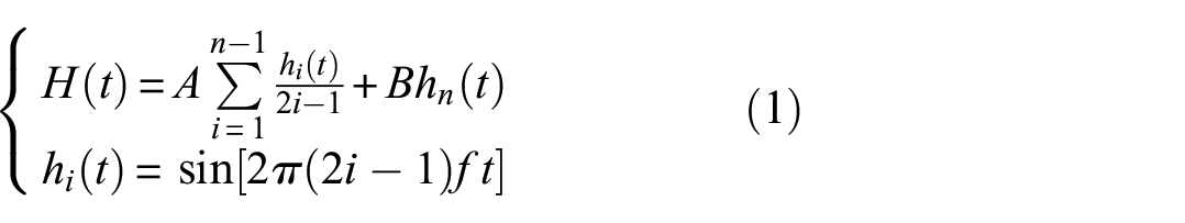
where A is the basic amplitude, B is the highest harmonic amplitude, n is the number of harmonics, and f is the frequency of the harmonic excitation source.
In this work, n is 5, f is 100 Hz, A:B is 1:0.811, and the multiple-harmonic excitation magnetic field schematic is shown in Figure 1(d). Take a one-cycle high-frequency component as an example analysis; the multiple-harmonic excitation magnetic field is a superposition of the DC and AC excitation fields, as shown in Figure 1(c). The DC magnetic field magnetizes the pipe, which reduces its permeability and increases the skin depth of the AC excitation field. Meanwhile, the magnetic field intensity changes as o → n → o → m → o and the permeability of the pipe varies as μ0 → μ2 → μ0 → μ1 → μ0, where μ1 > μ0 > μ2, as shown in Figure 1(a) and (b). When the magnetic permeability of the pipe surface reaches μ2, the magnetic field can easily diffuse into the air. Conversely, when the magnetic permeability of the pipe surface reaches μ1, it prevents the diffusion of the induced magnetic field due to the flux concentrator effect. 24 Therefore, the multiple-harmonic excitation method can enhance the magnetic field amplitude, which is beneficial for identifying pipe defects.
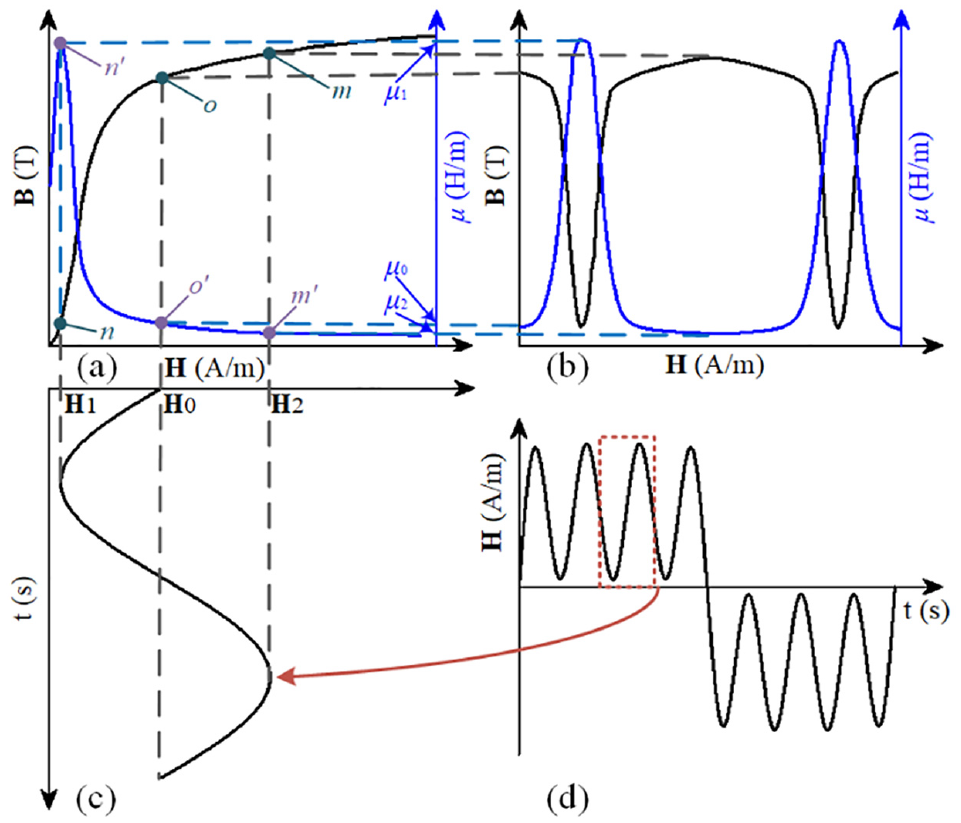
The detection principles of multiple-harmonic magnetic field: (a) magnetic induction and permeability of the pipe versus the magnetic field, (b) magnetic induction and permeability of pipes under multiple harmonic magnetic field excitation, (c) one-cycle high-frequency component from the multiple harmonic magnetic fields, and (d) multiple harmonic magnetic fields.
Probe design and principle
The probe consists of an excitation coil, two adjusting coils, and a group of pickup coils, as shown in Figure 2. The excitation coil generates the primary magnetic field, and the adjusting coils provide the auxiliary excitation field to focus the magnetic field. The pickup coil group consists of two induction coils connected in series and measures the change in magnetic flux density in the z-axis direction. To mitigate the coupling of the defect signal to the background signal, these two induction coils are connected in a differential manner and arranged at the position where the flux sum of the excitation field is zero. This configuration reduces the background signal intensity in the detection signal, which allows the preamplifier to work in a high dynamic range. With the system noise density and resolution remaining unchanged, the SNR of the defect signal is increased, resulting in higher defect detection resolution.
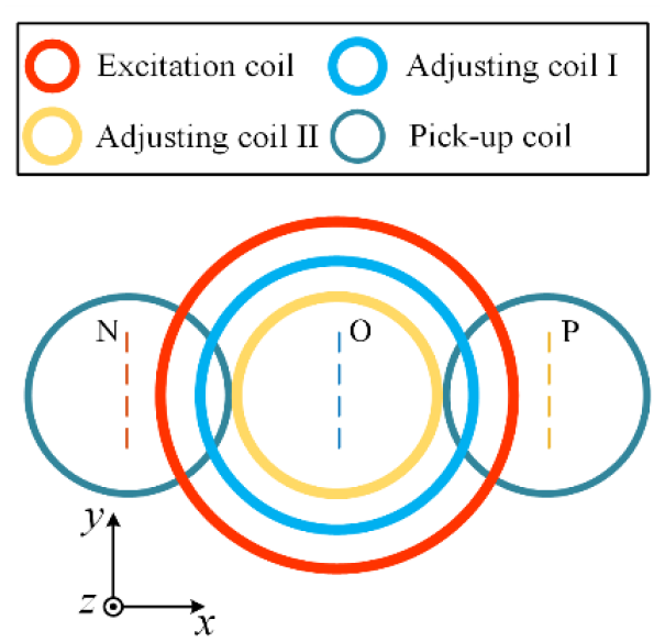
The structure diagram of the detection probe.
According to the electromagnetic detection principle, the excitation magnetic field induces eddy currents in the pipe, which generate an induced magnetic field. The induced magnetic field strength remains stable in defect-free regions of the pipe. In contrast, the induced magnetic field strength in the defect region is perturbed due to defects interdicting the eddy current flow path. 26 Therefore, measuring the magnetic field with the pickup coil group and analyzing the changes in the detection signal amplitude can detect pipe defects. The magnetic flux measured by each induction coil in the pickup coil group is the vector sum of the induced magnetic field and the excitation magnetic field, which can be expressed as:
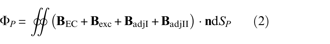
where ΦP,
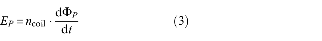
where ncoil is the turns of the induction coil. The detection signal output from the pickup coil is

where E P I and E P II are the electric potentials of two induction coils, respectively.
Algorithm description
Orthogonal phase-sensitive detection
The magnetic field detection signal measured by the probe is the vector sum of the excitation magnetic field, with the induced magnetic field being equivalent to the amplitude and phase modulation of the excitation magnetic field by the pipe. Without considering noise, the detection signal can be expressed as follows:
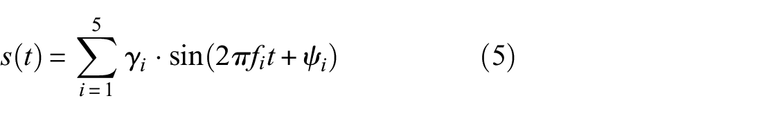
where γ i , ψ i , and f i are the amplitude, phase, and frequency of the ith harmonic component in the detection signal, respectively. A more detailed explanation of Equation (5) can be found in Appendix A. The detection signal consists of several harmonic components, and the amplitude of each harmonic component carries information about the pipe’s health. To identify the pipe defects, the amplitude data γ i needs to be extracted from detection signal. Therefore, two orthogonal reference signals with frequencies f j are introduced:
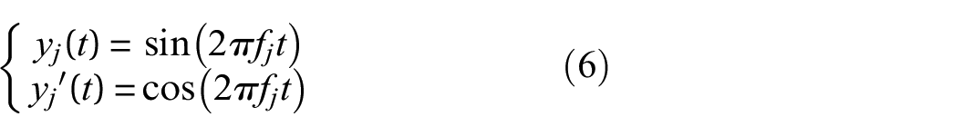
According to the trigonometric orthogonality property, when f j is equal to the ith harmonic frequency f i , the inner product of the detection signal and the reference signals can be expressed as:
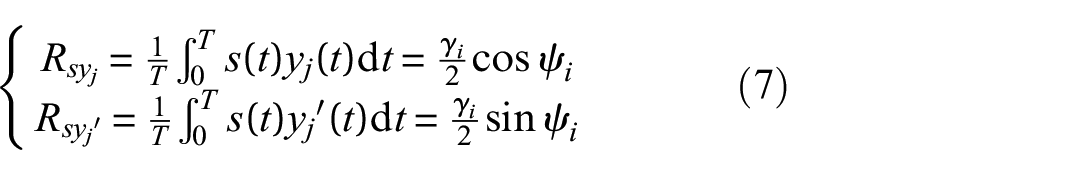
where T = 1/f is the period of harmonic excitation source. A more detailed explanation of Equation (7) can be found in Appendix B. Then, the amplitude γ i of ith harmonic is
By analyzing the variation in the amplitude data of the detection signal, pipeline defects can be localized. However, since the change in the induced magnetic field at the defect is too weak to produce a significant variation in the detection signal, especially when minor defects, the amplitude data cannot effectively reflect the pipe defect characteristics amidst substantial noise interference. Therefore, further processing of the amplitude data is required to improve the identifiability of the pipe defects.
Signal focus enhancement technology
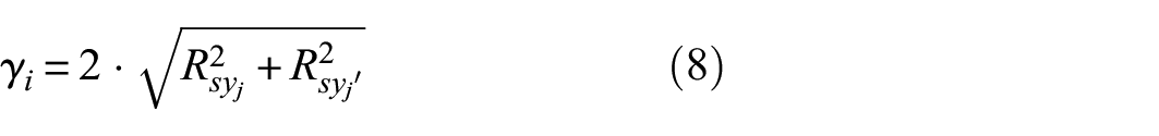
To effectively identify the pipeline defects, the signal focus enhancement technology (SFET) is proposed to extract magnetic field signal amplitude data under strong noise interference. The pipeline defect model is introduced here to illustrate SFET, As shown in Figure 3(a). The probe is moved horizontally along the y-axis with height H; its coordinates
Schematic diagram of SFET algorithm. SFET: signal focus enhancement technology.
When the probe is at

where
As described in “Probe design and principle” section, the pipeline generates an induced magnetic field under the magnetic field excitation, which is the vector sum of the induced magnetic fields generated by all pipe dipoles in the radiation region A
j
. When a defect exists in the A
j
, the induced magnetic field strength generated by the pipe dipoles is perturbed, which causes a change in the amplitude of the detection signal. However, the exact location of the defect cannot be determined. Therefore, it is assumed that all dipoles in
The pipe dipole corresponds to the position point
Since the number of pipe dipoles corresponding to the detection area at
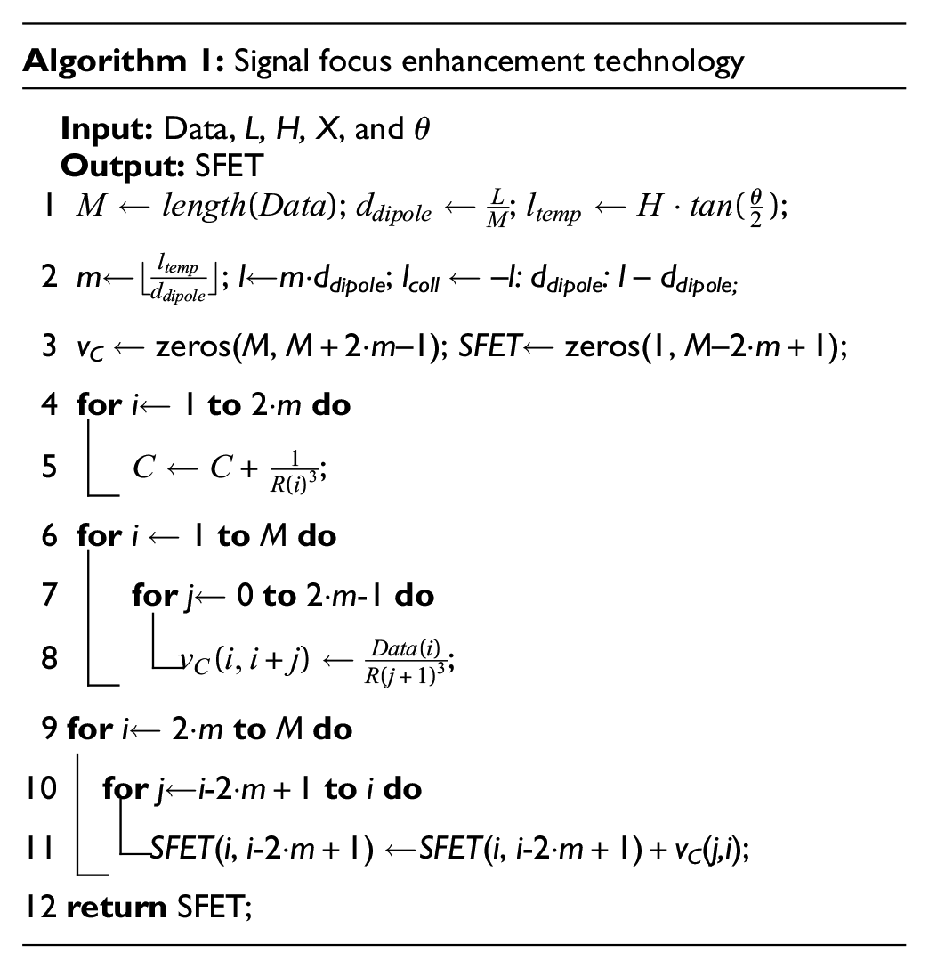
In the SFET algorithm, lift-off height H, offset distance X, and detection distance L are the same as in the actual detection situations. The parameter that needs to be set is the radiation angle β, which determines the size of the radiation region A j and needs to be set in combination with the sensor’s sensitivity. Suppose the sensor’s sensitivity is low, and the radiation angle is set large. In that case, the sensor may not detect the induced magnetic field changes generated by the pipeline dipole at the edge of the detection region, which will reduce the amplitude of the energy index at the pipe defect location. In addition, according to the smoke ring law, 27 the current loop generated by the excitation coils spreads downward at 94°, which the radiation angle should not exceed.
Numerical analysis
Induced magnetic field model
The pipe can be modeled as several superimposed magnetic dipoles based on the finite element analysis method. Then, the induced magnetic field generated by the pipe is the vector sum of the induced magnetic field generated by each magnetic dipole, which can be expressed as:
where μ is the magnetic permeability of the pipe,
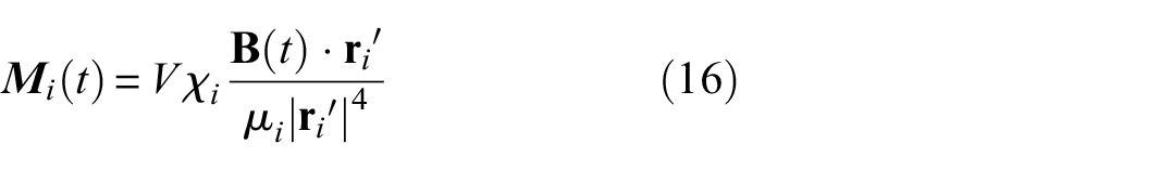
where V is the volume of the simulated defect, χ
i
= μ
r
− 1 is the magnetization rate of the pipe at the position i,
where μ
r
is the relative permeability of the pipe,
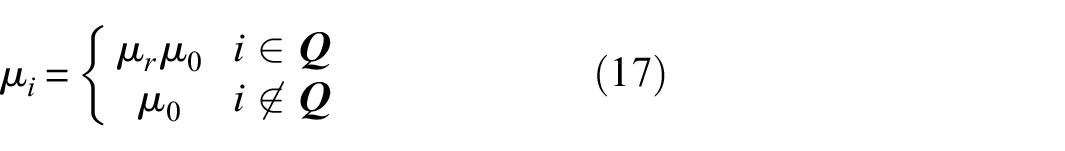
A pipe with a width × depth = 3 × 2 mm circumferential defect in the center was modeled, and the induced magnetic field was calculated using the forward simulation parameters (see Table 1). To visualize the location of the pipe defect, the probe is assumed to move at a constant velocity in the numerical model, and the distance is used instead of time to represent the x-axis in the simulation results. As shown in Figure 4, the amplitude of the induced magnetic field at the defect decreases rapidly and then recovers with increasing distance from the defect, which is consistent with the diffusive nature of the magnetic field.
Forward simulation parameter.
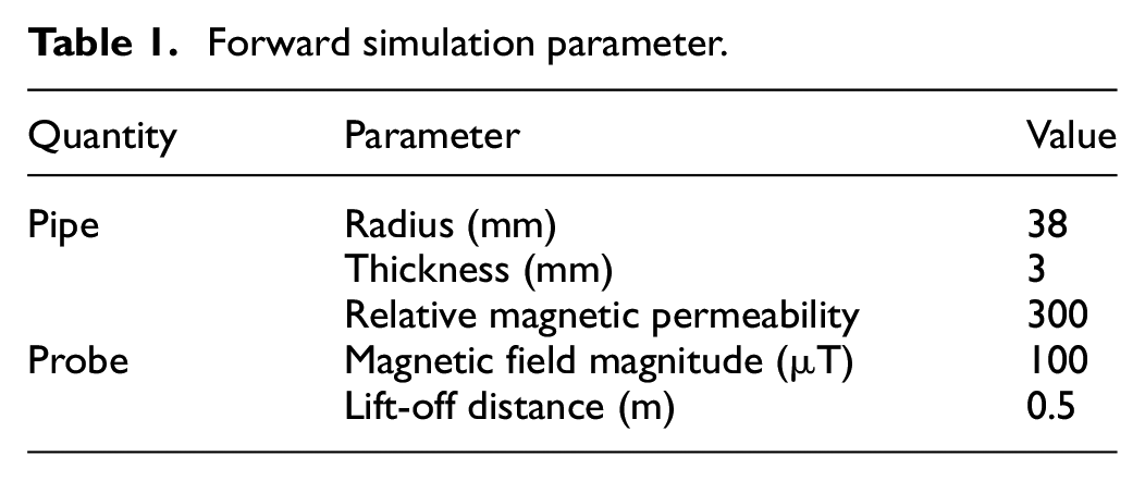
Magnetic induction signal model of the pipe with flaw: (a) magnetic induction curve diagram and (b) frequency domain diagram.
Simulation signal construction
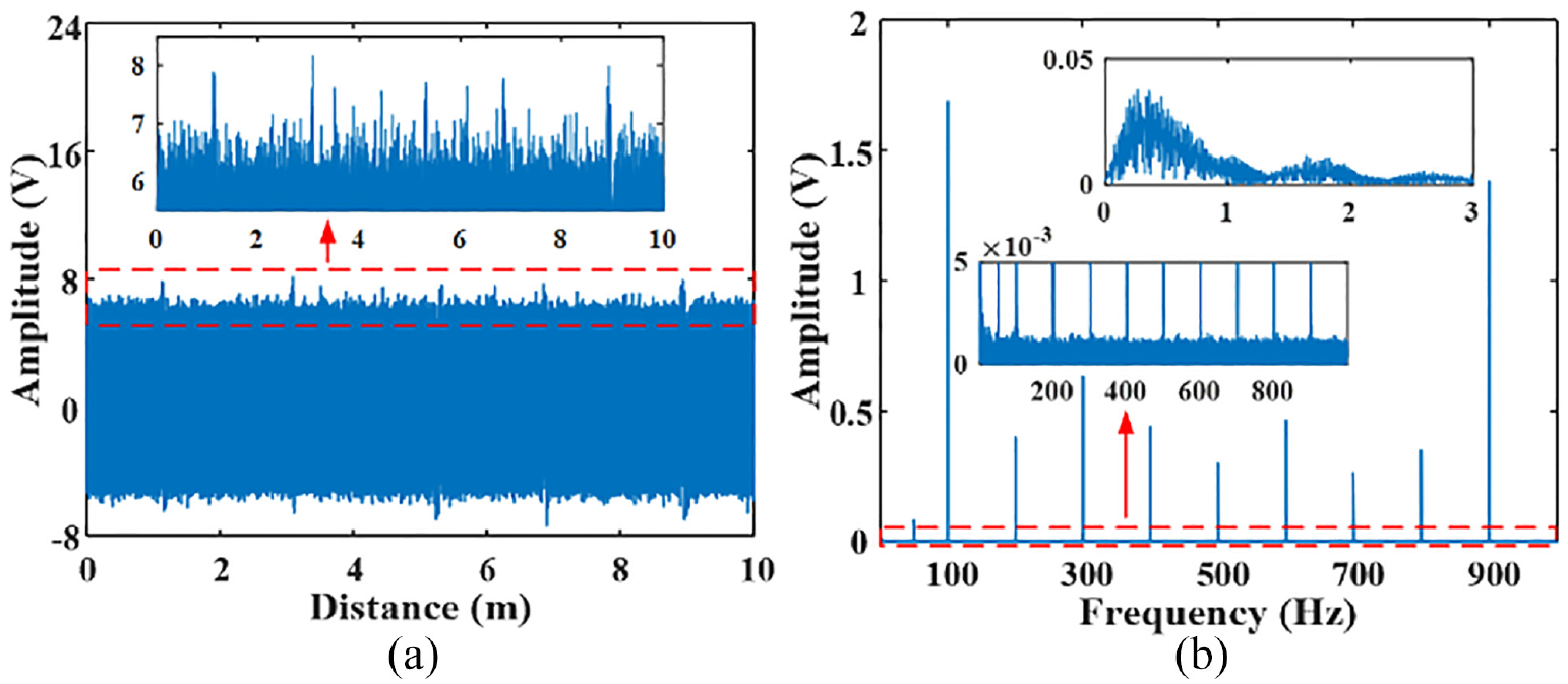
The simulation signal should incorporate all possible noises to make the numerical simulation analysis closer to the real engineering conditions. In addition to random noise and background signal, it is found that the probe can be disturbed by power frequency noise caused by the utility power supply, even harmonic noise caused by nonlinear devices in the excitation source instrument, and quasi-pulse type noise caused by probe jitter during movement. Therefore, the simulation model is constructed as follows:
In Equation (18), η = G·n·S P is the system factor (refer to Equations (2) and (3)), where G is the preamplifier gain, and the value of η here is set to 10e 6 . x2(d) is the excitation magnetic field signal, whose waveform is described by Equation (1). Due to probe manufacturing errors, the detection signal contains a high-intensity excitation magnetic field component, especially at high amplifier gains. Therefore, a 3.5 V excitation magnetic field signal was simulated.
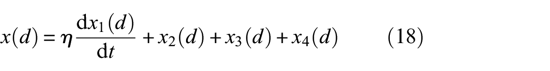
x 3(d) is the synthetic noise model, including random noise, power frequency noise, and even harmonic noise. We generated 5 dB of strong Gaussian white noise to simulate random noise, 15 dB of second, fourth, sixth, and eighth harmonic noise, and 30 dB of power frequency noise. As shown in Figure 5(a), there is no apparent change rule in the noise source, and the power frequency noise and even harmonic noise are entirely submerged in the random noise. As can be seen from Figure 5(b), the synthetic noises have an extensive frequency band range, and the primary frequency components are 50, 200, 400, 600, and 800 Hz.
The synthetic noise signal model: (a) synthetic noise curve diagram and (b) frequency domain diagram.
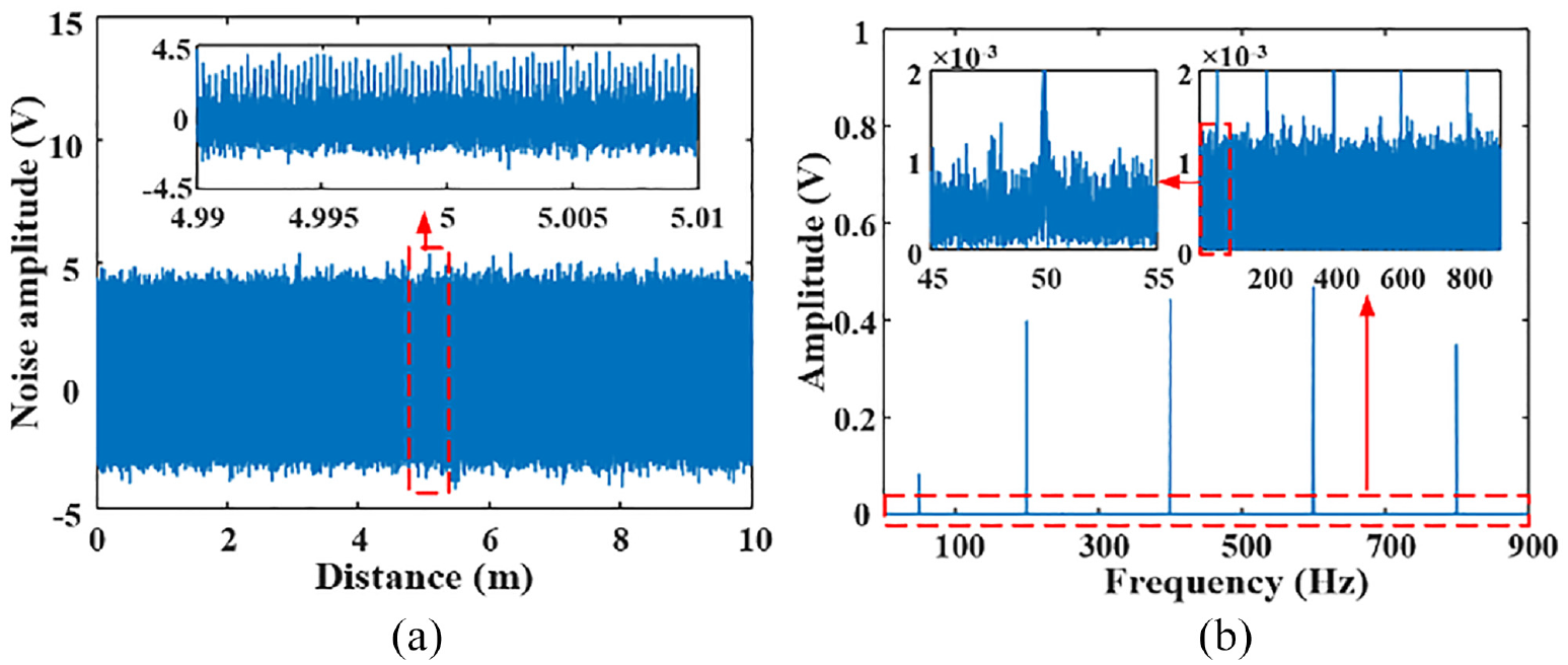
x 4(d) is the noise model caused by the probe jitter. According to previous experience, this noise is a quasi-pulse type signal, and we generated five jitter noises at 1.2, 3.1, 5.3, 6.9, and 9 m. As shown in Figure 6, jitter noise has a wide-frequency band range and most energy is concentrated in the low-frequency part as low as 1 Hz.
The probe jitter noise signal model: (a) jitter noise curve diagram and (b) frequency domain diagram.
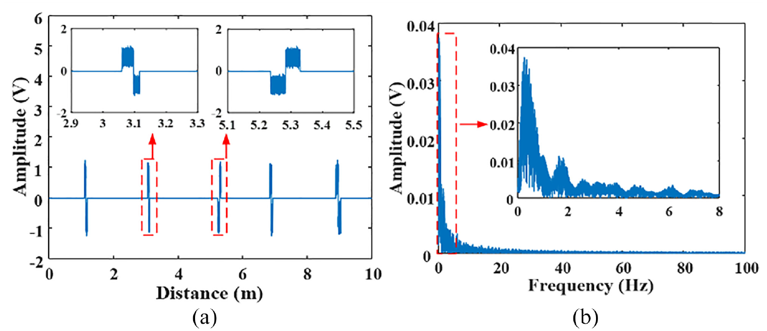
The multiple-harmonic magnetic field simulation signal is shown in Figure 7. The noise interference is evenly distributed throughout the simulation signal, and the jitter noise is distributed only for a while with considerable amplitude. Unlike the pipe-induced magnetic induction signal (see Figure 4), the defect feature in the simulation signal is entirely submerged in noise, which cannot directly determine the existence of a pipe defect.
Multiple-harmonic magnetic field detection signal model: (a) magnetic induction curve diagram and (b) frequency domain diagram.
Simulation signal analysis
The simulation signal and the noiseless signal (simulation signal without x3 and x4) are processed by the orthogonal phase-sensitive detection (OPSD) to obtain the amplitude data of the 100 Hz harmonic component. Then, the amplitude data is processed by the SFET (see Algorithm 1), and the radiation angle of SFET is set to 90°. The amplitude extraction results are shown in Figure 8. Here, the SNR and root mean square error (RMSE) are introduced to evaluate the performance of the proposed algorithm:
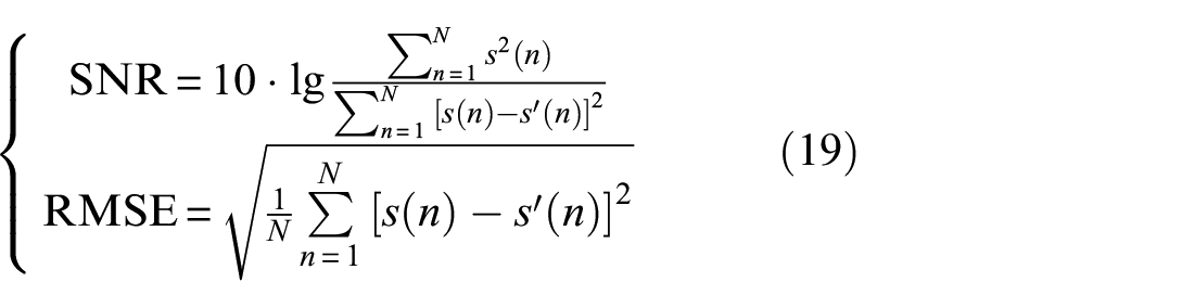
where s(n) is the noiseless signal, s′(n) is the simulation signal, and N is the length of the signal.
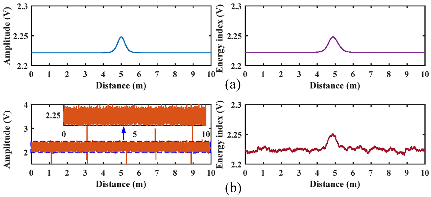
Processing results of OPSD and SFET: (a) noiseless data processing results and (b) simulation data processing results. OPSD: orthogonal phase-sensitive detection; SFET: signal focus enhancement technology.
Combined with Figure 8 and Table 2, although OPSD can improve the SNR and RMSE, the intense noise still drowns the weak flaw feature, making it impossible to observe the defect from the amplitude curve directly. The SFET can improve the SNR significantly, and the energy index curve peak caused by the flaw becomes prominent.
Evaluation index.
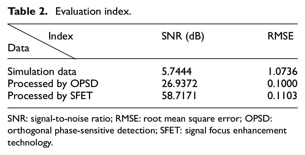
SNR: signal-to-noise ratio; RMSE: root mean square error; OPSD: orthogonal phase-sensitive detection; SFET: signal focus enhancement technology.
Experimental research
Experimental platform
The laboratory test platform is shown in Figure 9. The detection system comprises a power excitation source and an acquisition and storage module. The power amplifier module features a bridge-tied-load design, delivering an output power of 300 W and a peak-to-peak voltage of 60 V, and the acquisition and storage module includes a built-in quadruple oversampling capability with a sampling rate of 36 kHz. The excitation coil of the probe has a diameter of 400 mm, while the adjusting coils of the probe have diameters of 350 and 200 mm, each with 200 turns. The preamplifier is equipped with first-order bandpass filters with 30 Hz and 1.5 kHz cutoff frequencies and a gain of 310. The test pipes are two 45# steel pipes, P1 and P2, with a length of 360 cm, a diameter of 76 mm, and a wall thickness of 3 mm. An annular weld is in the center of P1, and an oil theft valve is in the center of P2.
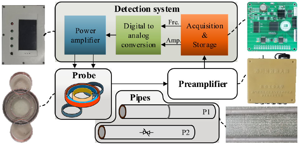
Test platform schematic diagram.
Experiment analysis
In this section, the performance of the proposed algorithm is verified through three laboratory test cases, including pipeline localization, weld localization, and oil valve localization, as well as a field experiment case of pipe defect detection.
Pipeline localization
The situation of several pipeline parallel paving is common. In this case, the two-pipe localization is used as a typical example of parallel pipeline localization, and the single-pipe localization is used for comparison. The two pipelines are laid parallel at a distance of s, and the probe moves horizontally along the detection guideline perpendicular to the pipeline, as shown in Figure 10. The detection distance is 300 cm, and the lift-off height H of the probe is 450 mm, which is about six times the diameter of the pipeline. Then, the localization tests for parallel pipelines with s of 150, 300, 450, and 600 mm, as well as for a single pipe, were carried out separately.
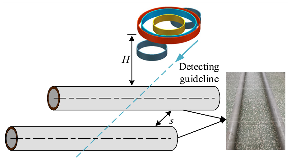
Pipeline localization test schematic diagram.
The parallel pipeline localization signal of 150 mm is used as an example. The OPSD algorithm is employed to obtain the 100 Hz harmonic component amplitude. The amplitude curve and its gradient curve are shown in Figure 11(a). Next, the amplitude data are processed by the SFET algorithm. Given the pipeline as a sizable magnetic source object, the detection signal has a high SNR and significant amplitude variation, allowing the radiation angle of the SFET to be set small. Consequently, the radiation angle in this case is set to 10°, and the energy index curve and its gradient curve are shown in Figure 11(b). Considering that the practical focusing distance in the SFET algorithm is smaller than the detection distance, it is necessary to remove the data on both sides of the energy index, and 250 cm is used here as the practical focusing distance. By comparing the gradient curve, it is evident that the energy index curve has less noise interference. Additionally, its gradient curve exhibits two peaks at the trough, indicating the presence of two pipelines. This inference cannot be made from the amplitude’s gradient curve, highlighting the SFET algorithm’s effectiveness in suppressing noise interference and extracting signal features.
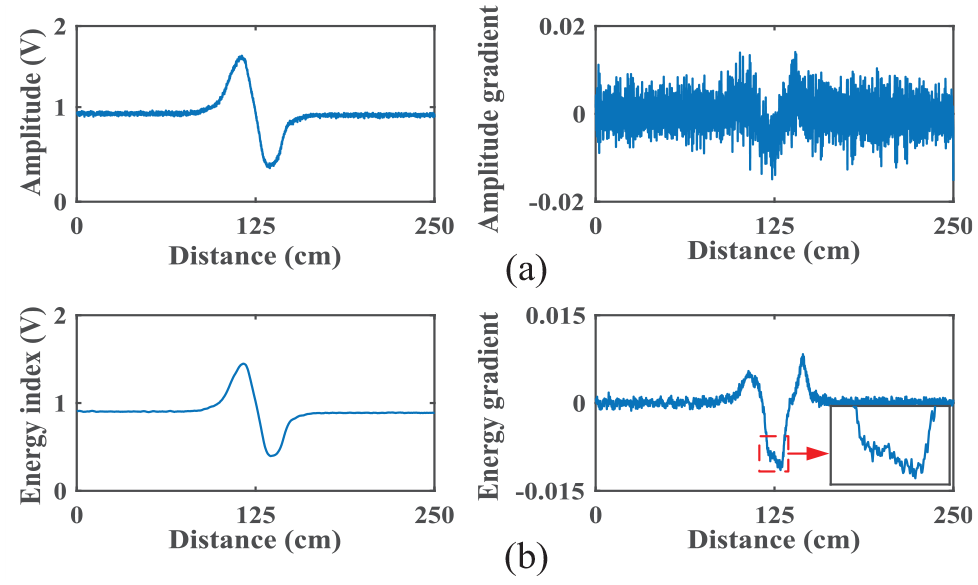
Pipeline localization results with the spacing of 150 mm: (a) amplitude signal obtained by OPSD and its gradient curve (b) energy index after enhanced by SFET and its gradient curve. OPSD: orthogonal phase-sensitive detection; SFET: signal focus enhancement technology.
The other localization tests were performed sequentially, maintaining all detection parameters consistent, and the results are shown in Figure 12. The results indicate that the proposed data processing algorithm can characterize the location of the pipelines. Furthermore, the gradient curve of the amplitude data can be used to determine the number of pipelines.
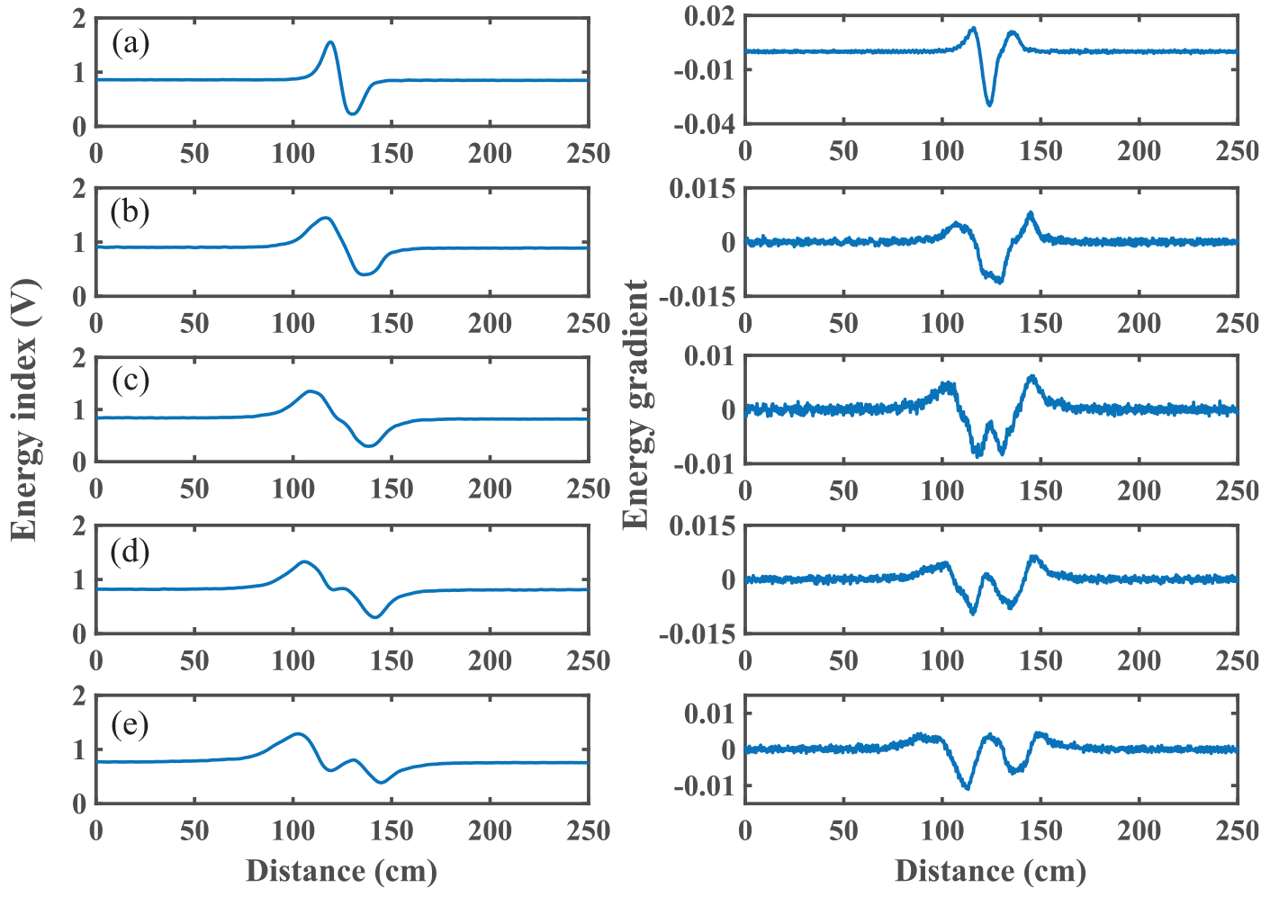
Pipeline localization result based on SFET and its gradient curve: (a) single pipe, (b) parallel pipe with a spacing of 150 mm, (c) parallel pipe with a spacing of 300 mm, (d) parallel pipe with a spacing of 450 mm, and (e) parallel pipe with a spacing of 600 mm. SFET: signal focus enhancement technology.
Single-pipe weld localization
Position the probe’s center line O and the pick-op coils’ center line N and P (see Figure 2) directly above the pipe, respectively. Move the probe horizontally along the detection guideline for weld localization, as shown in Figure 13. The detection distance is 360 cm, and the lift-off height H of the probe is 300 mm, which is approximately four times the diameter of the pipe.
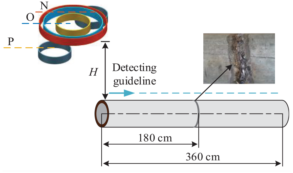
Weld localization test schematic diagram.
In contrast to pipeline localization, the background magnetic field signal and the induced magnetic field signal generated by the pipeline are considered noise in weld localization, while the induced magnetic field signal generated by the weld is the target signal. The reference signal frequency for OPSD is set to 100 Hz, the radiation angle of SFET is set to 60°, and 300 cm is used here as the practical focusing distance. As shown in Figure 14, not only can the weld be detected but also the side of the probe on which the weld is located can also be inferred from the trend of the energy index curve. This is because the pickup coil output is the difference between the electrical potentials of the two induction coils (refer to Equation (4)): the pickup coil output decreases when the weld is closer to the line N and increases when the weld is closer to the line P.
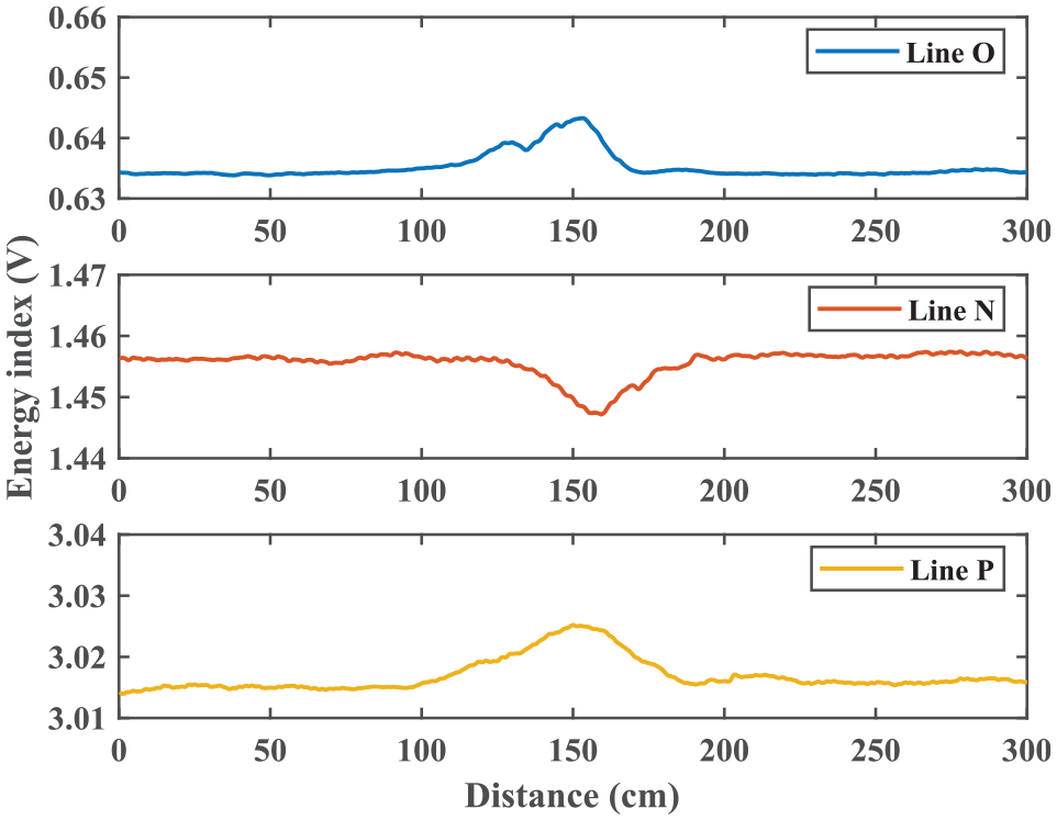
Weld localization result.
Parallel pipe oil valve localization
Position the probe in the middle of the two parallel pipelines and move it horizontally along the detection guideline parallel to the pipes to carry out the oil valve localization. As shown in Figure 15, the distance s between the pipes is 400 mm, the detection distance is 360 cm, and the lift-off height H of the probe is 300 mm, which is approximately four times the diameter of the pipe.
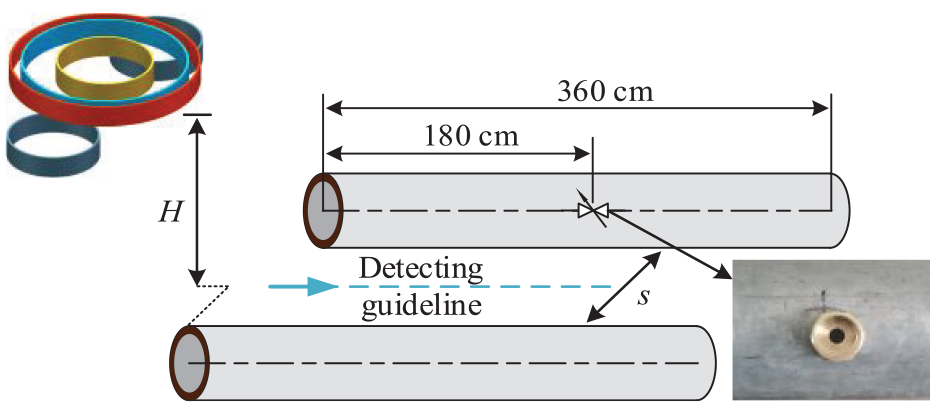
Oil valve localization test schematic diagram.
The signal-processing method and parameter settings are the same as in the single-pipe weld localization case, and the test results are shown in Figure 16. Compared with Figure 14, the energy index curve of oil valve localization is pronounced with minor fluctuations. This is because the induced magnetic field strength generated by the parallel pipeline and the oil valve is strong and stable, making a low noise ratio in the detection signal and significant induced magnetic field variation at the oil valve.
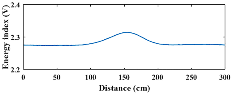
Oil valve localization result.
Single-pipe defect detection
To further verify the effectiveness of the proposed method, the probe was structurally encapsulated, and a field experimental platform was built, as shown in Figure 17(a). The experimental pipe is a 20# steel pipe with a length of 600 cm, a diameter of 76 mm, and a wall thickness of 10 mm. Three grooves were machined on the pipe to simulate corrosion defects, with dimensions of 15 × 30 × 3 mm (groove I), 25 × 30 × 3 mm (groove II), and 30 × 30 × 3 mm (c) (groove III), as shown in Figure 17(b). The probe was positioned above the pipe and moved horizontally along the detection guideline parallel to the pipe for defect detection. The detection distance is 550 cm, and the lift-off height H of the probe is 230 mm, approximately three times the diameter of the pipe.
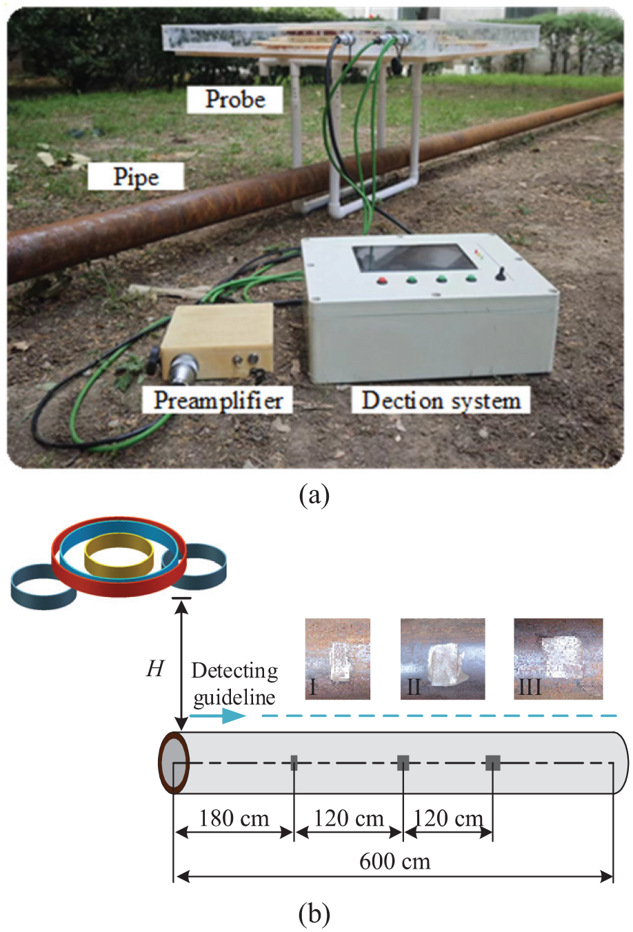
Defect detection experiment: (a) field detection photograph and (b) defect detection schematic diagram.
Similarly, the amplitude data of the 100 Hz harmonic component was obtained using the OPSD, the radiation angle of SFET is set to 75° considering the weak change of induced magnetic field at the defect, and 500 cm is used here as the practical focusing distance. As shown in Figure 18, the energy index at the defective pipeline changes significantly, and the degree of damage can be characterized by this change in the energy index, verifying the effectiveness of the proposed defect signal extraction method.
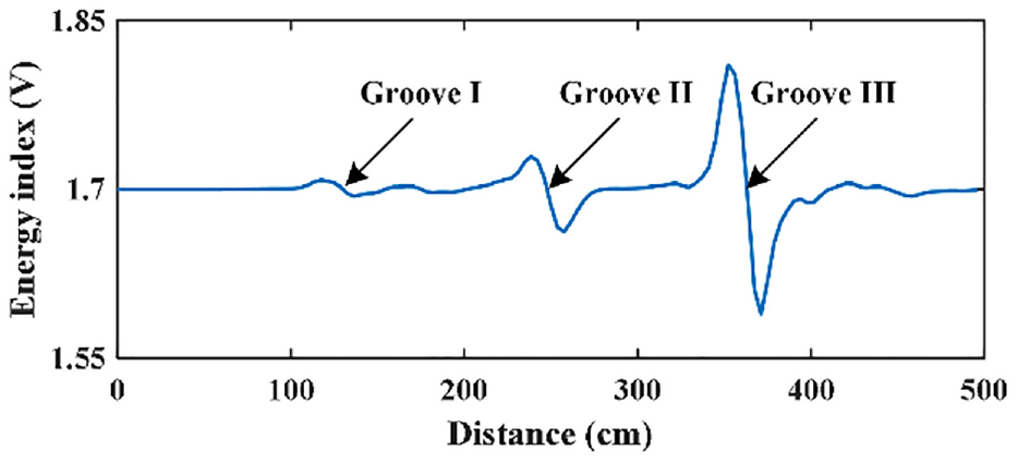
Pipe grooving defect detection result.
Discussion
This section presents an empirical summary and provides the following recommendations based on the above research and experimental results.
Noise sensitivity
A denoising method is introduced to demonstrate that the SFET algorithm is insensitive to noise, as shown in Figure 19. First, sum the periodic signals and compute their average. Next, invert the second half-period of the signal within one period and average it with the first half-period. Finally, the half-period signal is restored to a full periodic signal. This method can eliminate even harmonic and power frequency noise and reduce the random noise by
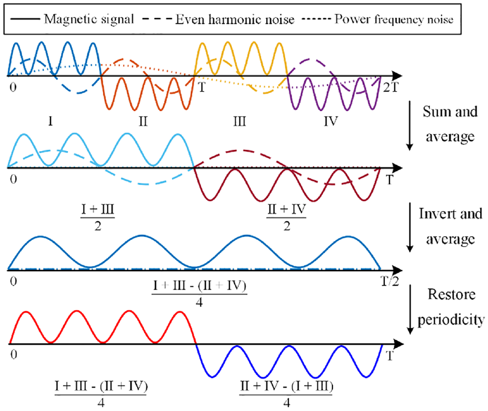
Schematic diagram of noise cancellation method.
The same method and parameters were used to process the oil valve detection data after denoising the proposed method. The result is shown in Figure 20. The energy index value of the denoised data is the same as that of the raw data. However, the denoising process is helpful. As shown in the energy gradient diagram, the tiny fluctuations in the energy index of the denoised data prove that most of the noise has been removed. It is beneficial for further processing the data in a noisy environment, such as using the energy index gradient data for defect classification combined with neural network algorithms.
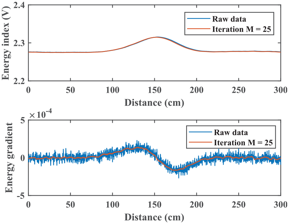
Result comparison between denoising data and raw data.
Detail resolution
The radiation angle setting in the SFET algorithm is flexible: the small radiation angle provides an energy index signal with higher resolution, while a huge radiation angle provides an energy index signal with higher SNR. The radiation angle of the parallel pipes spaced 150 mm case in the Pipeline Localization experiments is set to 30° and compared to the processed results with a radiation angle of 10°. As shown in Figure 21, the energy index fluctuation rate is lower with a larger radiation angle, which is suitable for extracting weak feature signals. However, the gradient of the energy index follows the same trend as that of the energy index of the single pipeline localization test, making it impossible to differentiate the parallel pipeline. It can be seen that the SFET algorithm acts as a filter, and the large radiation angle can easily filter out the detailed information. Therefore, it is recommended that the radiation angle of the SFET be set smaller while slowing down the detection speed when focusing on detection details. While detecting minor defects, the radiation angle of the SFET can be set larger, which can help suppress noise interference and enhance defect features.
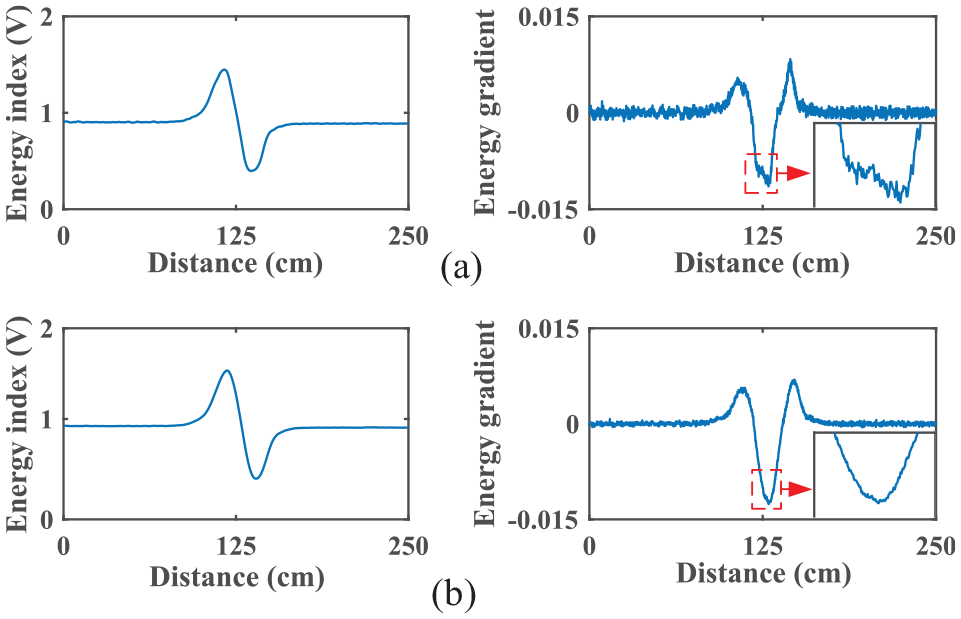
Comparison of results for different radiation angle parameters: (a) radiation angle is 10° and (b) radiation angle is 30°.
Weak signal extraction
The proposed algorithm flow can be improved when detecting weak defect signals in a robust interference environment. For example, the OPSD calculates each harmonic magnetic detection signal frequency component. Then, the amplitudes of each frequency component are normalized and fused. Finally, the fused amplitude data is processed by the SFET algorithm. Take the Parallel pipe oil valve detection as an example, and the result is shown in Figure 22. The background energy has been manually subtracted from the results to facilitate comparison. The signal amplitude at the oil valve has increased by about one-third, proving that the improved method also contains more target characteristic information, which helps to detect weak signals. However, as shown in the energy gradient diagram, the improved algorithm has a significant fluctuation rate of energy indicators, indicating that the improved algorithm contains more noise signals. Therefore, an effective denoising process should be performed when using the improved algorithm to ensure the signal has a sufficiently high SNR.
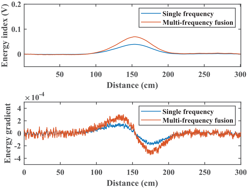
Comparison between single-frequency component extraction result and multi-frequency fusion extraction result.
Energy index description
The proposed defect signal extraction method is based on the universal electromagnetic NDT principles. It allows for comparing damage levels within the same detection sample, as demonstrated in single-pipe defect detection experiment. However, the single-pipe weld localization experiment shows that the magnitude of the energy index varies significantly depending on the position of the weld relative to the probe. This variation is caused by the induction coils’ installation position and connection form, which the proposed algorithm does not account for the effect of the probe structure on the energy index. Therefore, using the energy index to compare damage levels between different detection samples is not rigorous.
Conclusion
This research presents a noncontact defect signal extraction method and validates it using multiple-harmonic magnetic field detection technology. First, the OPSD algorithm is proposed to obtain the detection signal’s amplitude to characterize the defect signal features. Then, the SFET is proposed to enhance the defect signal features in response to the issue of low defect identification accuracy caused by high-density noise interferences. Unlike the defect signal extraction method based on time-frequency analysis and filtering algorithm, the proposed method is insensitive to noise because it does not exploit the detection signal and noise’s time-frequency characteristics and acts as a filter itself during data processing. Next, the simulation signal based on the induced magnetic field model of pipe defect and noise model was constructed to analyze the proposed algorithm. The simulation results demonstrate that the proposed method can identify defects from signals with a low SNR of 5.7 dB. Finally, the experimental platform was built, and three laboratory test cases and a field experiment case were conducted. The test results show that the proposed algorithm can accurately locate the pipe, weld, and oil valve positions with considerable resolution. The experiment result shows that the change in the energy index amplitude can reflect the extent of pipe damage.
Overall, the proposed defect signal extraction method is a promising method for fast detection of various anomalies in noncontact electromagnetic detection, which can be widely used in buried pipeline detection, pipeline detection without removing cladding, geophysical electromagnetic exploration, and others. Future work will utilize the proposed method for quantitative analysis and risk assessment of pipeline defects. This work will include a method for determining the optimal radiation angle parameter in the SFET algorithm and an improved defect signal extraction method in conjunction with the probe model to enable quantitative comparisons of the extent of pipe damage between different detection samples.
Footnotes
Appendix A
The excitation magnetic field signal contains several independent harmonic signals, and the induced magnetic field signal is a superposition of the amplitude and phase modulation of each harmonic signal by the pipeline. Therefore, the detection signal can be expressed as:
Where h i is the ith harmonic excitation magnetic field signal in the detection signal, with the amplitude of λ i ; h i ′ is the ith harmonic induced magnetic field signal in the detection signal, with amplitude α i and phase θ i ; f i is the frequency of the ith harmonic component. Since each harmonic component is independent of the other, the superposition signal s i of the ith harmonic excitation magnetic field signal and the ith harmonic induced magnetic field signal is analyzed as an example, and its expression is given by:
According to the sum and difference formula of trigonometric functions, Equation (A2) can be expressed as
According to the basic equation of trigonometric functions, Equation (A3) can be written as
Bringing Equation (A4) into Equation (A1), the detection signal can be expressed as
where
When the probe structure is fixed, the amplitude λ i of ith harmonic excitation magnetic field signal remains constant; the change in amplitude α i of ith harmonic induced magnetic field signal reflects the degree of pipe damage. Therefore, pipeline defect detection is achieved by analyzing the variation in amplitude γ i of the detection signal.
Appendix B
The OPSD algorithm utilizes the trigonometric functions’ orthogonality property to extract the target frequency harmonic amplitude data in the detection signal. Based on this property, the inner product of the detection signal and two reference signals in the period [0, T] of the harmonic excitation source can be expressed as:
According to the trigonometric sum and difference formula, Equation (B2) can be written as:
where
Since T is the harmonic excitation source period, which is (2i−1) times the period of the ith harmonic. Therefore, when f j is equal to the ith harmonic frequency f i , the integrals over Equation (B3) to Equation (B6) are
When f j is not equal to the ith harmonic frequency fi, T is |2i − 2j| times the period of the sine signal or cosine signal with frequencies |f i + f j | and |f i − f j |. Therefore, the integrals over Equation (B4) to Equation (B7) are
Bringing the Equation (B7) to Equation (B14) into Equation (B2), then, the correlation function is solved as
This approach allows for the extraction of the amplitude and phase of each harmonic component from the detection signal, providing essential information about the health status of the pipeline.
Declaration of conflicting interests
The author(s) declared no potential conflicts of interest with respect to the research, authorship, and/or publication of this article.
Funding
The author(s) disclosed receipt of the following financial support for the research, authorship, and/or publication of this article: This work was supported by the National Key Research and Development Program of China (grant no. 2017YFC0805005-1) and the Key Project of Beijing Municipal Education Commission (grant no. KZ2018 10005009).