Recursive parameter estimation for the on-line monitoring of delamination growth in composite structures

Abstract

One of the main failure phenomena in composite materials is delamination, which consists of the progressive separation of plies. An augmented extended Kalman filter (KF) approach for joint input-parameter estimation is proposed and demonstrated in this work for delamination growth monitoring. In particular, a novel recursive estimation scheme for parameter identification is proposed within the joint input-parameter scheme which allows for a substantial reduction of the number of required sensors, enabling the use of the proposed KF approach. The proposed methodology also allows for the full-field response reconstruction, interface stiffness degradation monitoring and critical load identification. The methodology is validated on both simulated as well experimental data of a carbon fiber double Cantilever beam specimen, showcasing good accuracy for both cases.

Keywords

Delamination growth composite materials damage monitoring Kalman filter input-parameter estimation

Introduction

Nowadays, laminated composites are widely used in primary and secondary structural components in aerospace industries. The failure and instability of composite materials are difficult to predict and occur due to several phenomena, including delamination, which can drastically lead to a reduction of the mechanical performances of the component. Delamination is a local phenomenon, and its monitoring during operation is extremely challenging. Despite the extensive work presented in literature on optimal sensor placement (OSP)^1–3 for structural health monitoring (SHM), a robust approach to select an optimal map of sensors for delamination growth monitoring during operation is not yet available due to the complexity of the phenomenon and the resulting high concentration of stresses and non-linear effects make the design of a monitoring system much more complicated. Different kinds of SHM techniques applied to composite structures have been explored in the recent literature and can be identified and classified into two main groups: model-based and sensor-based. Model-based methods undertake simulation data and compare the model with experimental signals in frequency or time-domain or even as modal parameters.^4,5 The main disadvantage of these methods is the requirement for prior knowledge from high-fidelity nonlinear finite element model (FEM) simulations or complex analytical solutions. In this case, model validation is expensive in terms of computation and experiments since local damage information can be mainly identified at high frequencies and this requires high model accuracy. The usage of models in these cases is thus challenging. To overcome this limitation, sensor-based methods can be considered to detect damage by comparing response signals with baseline measurements.⁶ Most of the recent studies presented in literature on SHM for composite materials focus on sensor technologies for online structural monitoring, for example, piezoelectric materials and sensors^7–9 and fiber Bragg gratings (FBGs),^10–12 in contrast to standard nondestructive test¹³ approaches which are usually employed by industries as offline damage monitoring. With the advance of machine learning in the field of structural mechanics and composite materials, several data-driven and physics-informed architectures have also been proposed^14–17 to solve the inverse identification problem from time-series data and frequency shifts in sensor signals. By summarizing the state-of-the-art regarding SHM for delamination growth monitoring, the following main limitations in the implementation of such techniques at industrial-scale level can be identified:

Limited works are presented in literature regarding the study of optimal sensors placement for the identification and monitoring of local effects;

Artificial intelligence-based methodologies outperform other techniques because of their ease of implementation as these require only sensor data. However, the need for training data is the most obvious limitation, especially in the field of composite structures where uncertainties play an important role;

Model-based approaches are of limited usage due to the required level of accuracy in FEM;

Limited focus on the identification of critical loads causing failure in composite laminates.

This contribution proposes an estimation approach that relies on a trade-off between the amount of sensor data and level of accuracy of the FE model to perform inverse system identification for delamination growth monitoring. A well-known approach is the Kalman Filter (KF) which has been widely used for structural mechanical applications for the online identification of full-field response, external loads and physical parameters.^18–21 Moreover, OSP techniques for KFs have been developed to ensure an optimal estimation by employing a reduced set of sensors.²² When going towards FE modelling, a common approach is to reduce the computational cost by using model order reduction (MOR) techniques. However, it is important to underline that the implementation of MOR in KF requires some form of training data, depending on the nature of the system:

Linear systems: FE model calibration/validation in the frequency domain of interest which allows a direct eigenvalue analysis to compute the reduction basis.

Parametric or nonlinear systems: FE model calibration/validation within the full range of parameters/nonlinearities. Parametric model order reduction (pMOR) can be employed requiring a training scenario.^23–25

The proper orthogonal decomposition (POD) method is one of the most used and efficient approaches to calculate a reduction basis for nonlinear systems.²⁶ The main advantage of POD is that it employs on linear matrix operations, projecting the nonlinear system onto a subspace that allows to preserve the nonlinear dynamics. Moreover, POD is computationally efficient when compared to other pMOR techniques.²⁶ The main principle of the POD is in the selection of the meaningful shapes or modes of the solution corresponding to the full range of the parameter space. This contribution employs the POD method for the computation of the global reduction basis, starting from the concatenation of local bases. Each of the latter corresponds to the eigenvalue solution of the linearized model being evaluated for the sampled parameter values. The delamination can be associated to a local degradation of stiffness parameters of the model. The delamination curve is thus sampled and the corresponding linear models constitute the training scenario of the pMOR. This approach has the advantage that it avoids simulation of a nonlinear FE model which is computationally expensive and requires a complex formulation. Therefore, in this work a less time-consuming workflow for the on-line monitoring of delamination growth in composite materials is proposed by embedding pMOR into the KF, as demonstrated in literature²⁰ for an isotropic structure. Moreover, a novel recursive parameter estimation is proposed which allows to further reduce: (1) the computational cost associated to an increase of the number of estimated parameters and, (2) the number of sensors required to guarantee system observability. Some of the limitations mentioned above are thus addressed. A unidirectional carbon fiber double Cantilever beam (DCB) specimen is tested under static loading to validate the methodology using both simulated and experimental data. The target estimation quantities are the delamination growth, that is, decreasing of the interface stiffness, as well as the critical loads.

The motivations behind this work and research contributions are summarized as follows:

To the authors’ best knowledge, the employment of Kalman-based techniques for the online monitoring of delamination growth in composite materials is not yet addressed in literature. Preventing failure in composite structures is not trivial and a robust solution for operational life is still missing from literature. The work presented in this article for the monitoring of delamination growth in a small specimen is a first step towards the application of Kalman-based methods in the field of composite materials.

The applicability of a Kalman-based solution allows for the online detection and monitoring of delamination during flight conditions, which therefore allows to reduce maintenance costs and downtime due to manual inspections.

The KF estimation problem becomes intractable when the number of unknowns is too high, as it consequently requires a high number of sensors and therefore the computational cost increases substantially. This article presents a novel recursive parameter estimation approach that embeds pMOR, which allows the applicability of Kalman-based techniques for the estimation of high-dimensional parameter spaces. Even though the approach is demonstrated for the estimation of delamination growth monitoring, it can be applied and generalized to other fields as well, including the extension to multiple load estimation.

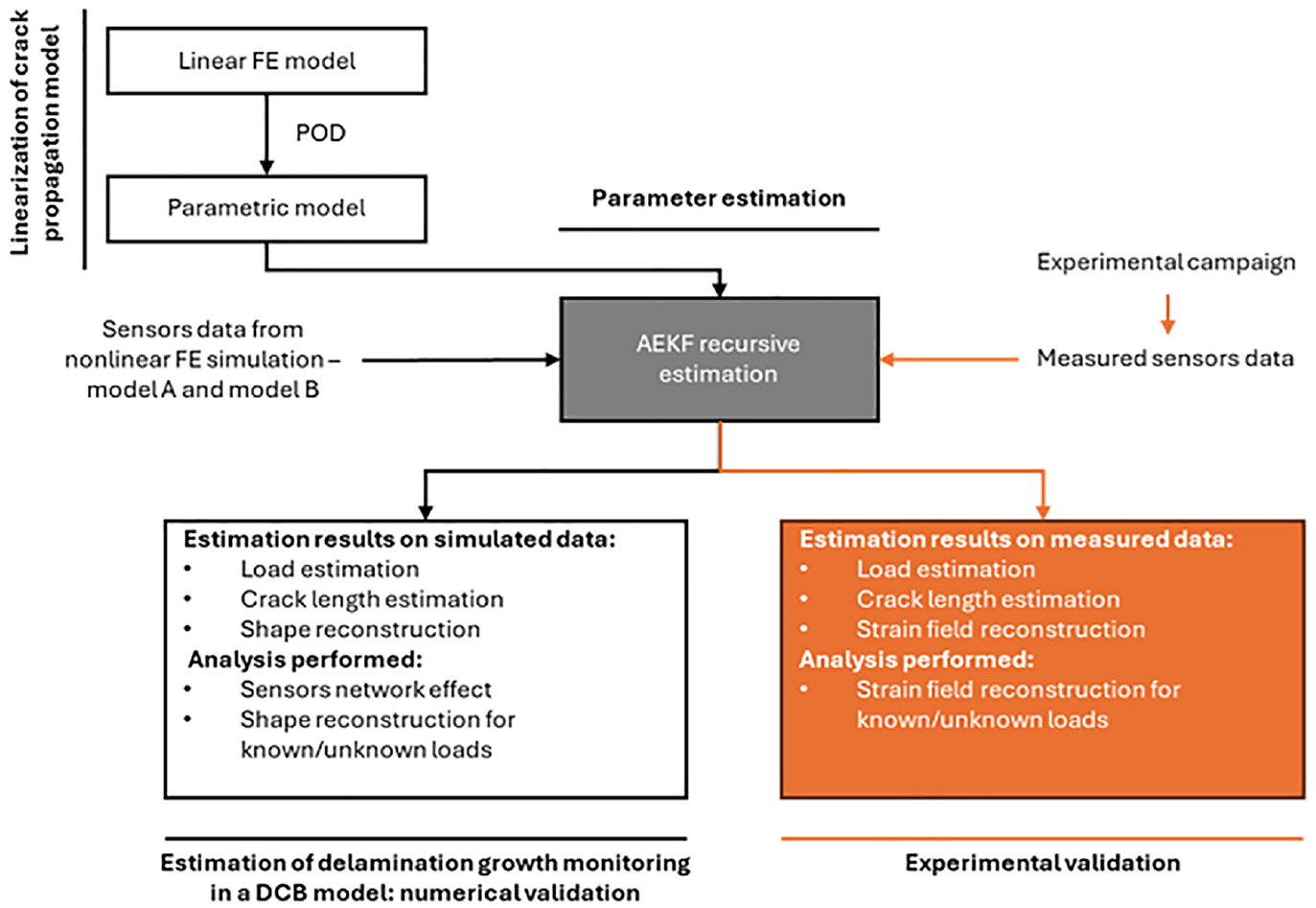
The remainder of this article is structured as follows and illustrated in the flowchart in Figure 1: “Linearization of the crack propagation model” section describes the linearized parametric FE model and the pMOR methodology, “Parameter estimation” section presents the Augmented Extended Kalman Filter (AEKF) recursive parameter estimation, “Estimation of delamination growth in a DCB model: numerical validation” section validates the estimation workflow with simulated data and studies the optimal number of sensors, “Experimental validation” section includes the experimental validation using a real DCB specimen instrumented with strain-gauges sensors and finally, “Conclusions” section discusses concluding remarks and future developments of the presented methodology for industrial-level applications.

Figure 1.

Flowchart of the paper structure.

Linearization of the crack propagation model

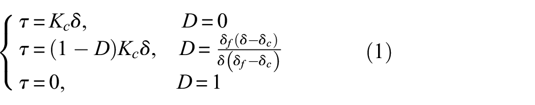
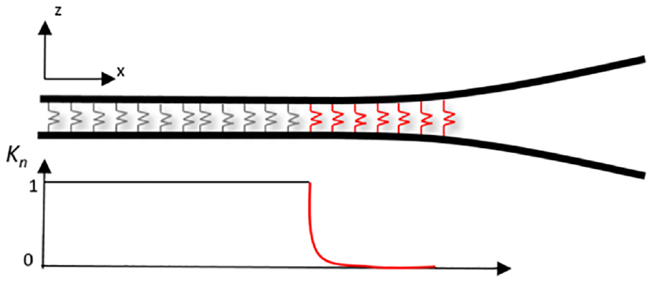
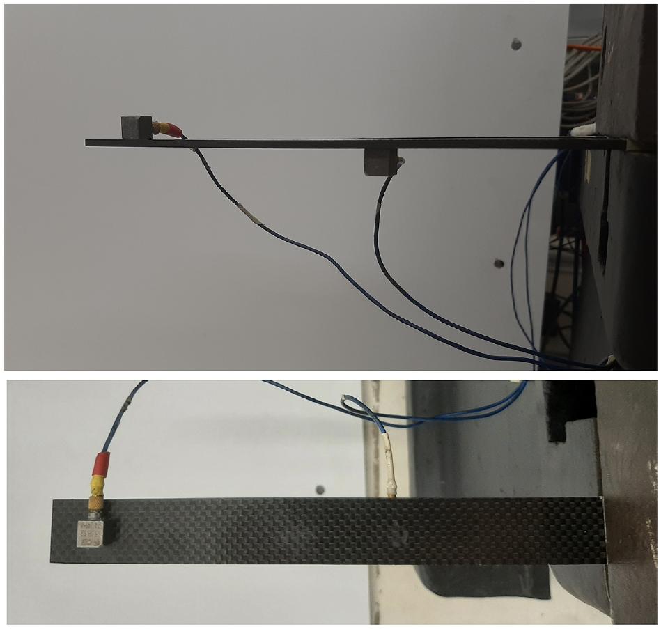
The mode-I interlaminar fracture toughness of a carbon fiber-reinforced plastic composite laminate is generally determined by testing a DCB specimen, in compliance with the EN 6033²⁷ standard. The test is performed as shown in Figure 2: the two arms, that is, cantilever beams, are pulled apart by applying a tip displacement in opposite direction and in quasi-static conditions. The initial crack present in the specimen will propagate along the specimen span until the sample breaks or the maximum displacement is reached. Figure 3 shows a schematical overview of the progressive propagation of the delamination in a DCB sample using a bi-linear interface cohesive law²⁸:

{\begin{matrix} τ = K_{c} δ, D = 0 \\ τ = (1 - D) K_{c} δ, D = \frac{δ_{f} (δ - δ_{c})}{δ (δ_{f} - δ_{c})} \\ τ = 0, D = 1 \end{matrix}

(1)

Figure 2.

Experimental DCB setup.

Figure 3.

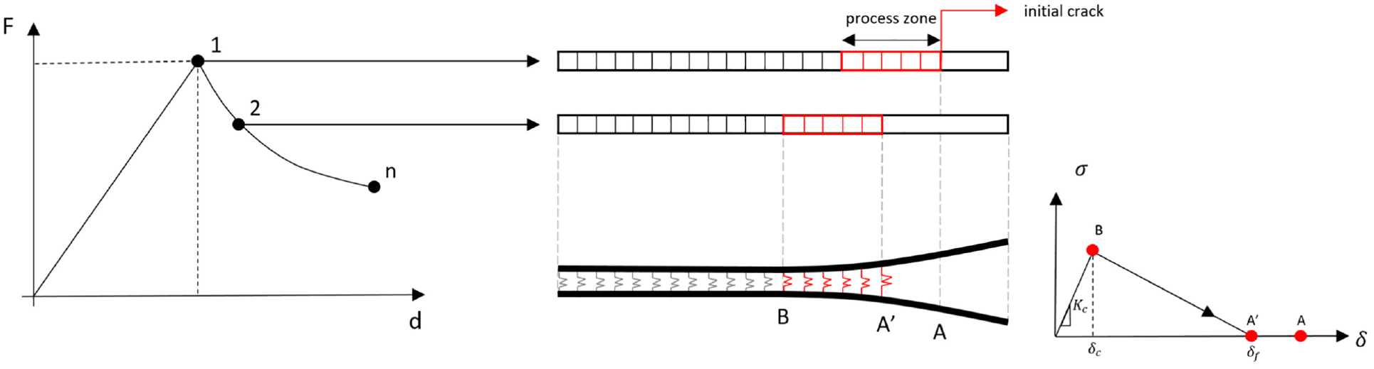
Schematic representation of the progressive delamination in a DCB model using a bi-linear cohesive law.

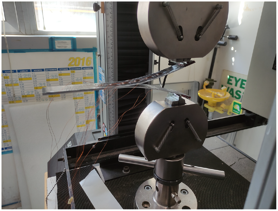
where $τ$ and $δ$ are the normal stress and displacement, respectively, $K_{c}$ is the interface stiffness, $δ_{c}$ and $δ_{f}$ are, respectively, the critical and the final interface displacements and $D$ is the damage variable. Once the critical stress in the first (virtual) interface element is reached—point 1 shown in Figure 3—the crack starts to propagate and all the elements in the process zone move to the softening region. Each elemental stress in the process zone lies on the $τ - δ$ curve, which is representative of the cohesive law of the normal opening mode I. The following significant points can be identified: (1) general element $A$ ahead of the crack tip shows a zero stiffness associated to the separation of the two arms in that point ( $D = 1$ ); (2) element $A^{'}$ is the current crack tip approaching the zero stiffness ( $D = 1$ ); (3) segment $A^{'} - B$ is the fracture process zone, where the linear-elastic behavior is exceeded and a gradual decreasing of the elemental stiffness is observed from point $B$ to point $A^{'}$ , (4) the segment O–B, where the elements exhibit a linear elastic behavior ( $D = 0$ ). Considering this representation of the crack and its relative fracture process zone, it turns out that each generic point of the $F - d$ curve of the DCB coupons can be represented by an equivalent linear elastic model as presented by Dimitri et al.²⁹ The FE model consists of two linear beams connected with interface elements as node-to-node springs. The springs from the specimen root to point $B$ are characterized by very high stiffness values, relative to the overall model, that is, $1.0 e^{6} \frac{N}{mm}$ , to represent the perfect bonding amount between the two coupon arms.

Parametric model

Given a linear elastic FE³⁰ model with $n_{d}$ number of degrees of freedom (DoFs), the equations of motion describing the system dynamics excited by the input load vector $u (t) \in R^{n_{u}}$ , can be formulated as:

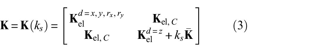
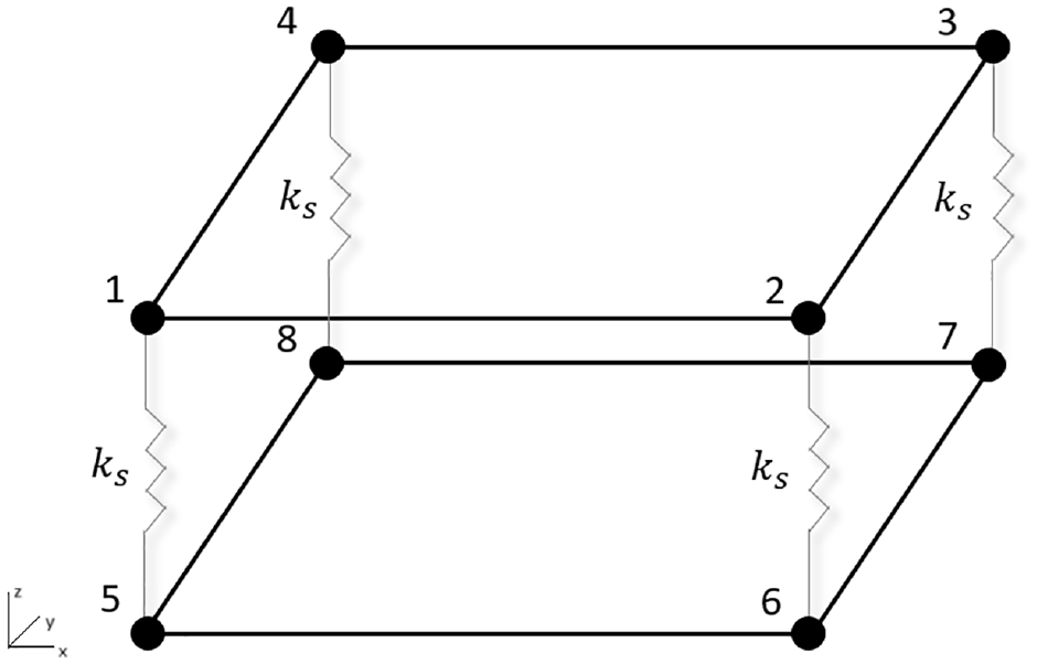
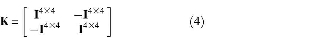
M \overset{\cdot\cdot}{z} (t) + C \overset{\cdot}{z} (t) + Kz (t) = Bu (t)

(2)

where $M \in R^{n_{d} \times n_{d}}$ , $C \in R^{n_{d} \times n_{d}}$ , $K \in R^{n_{d} \times n_{d}}$ are, respectively, the mass, damping, and stiffness matrices of the system, $B \in R^{n_{d} \times n_{u}}$ is the Boolean input shape matrix that distributes the inputs, that is, loads, over the DoFs of the system, $z (t) \in R^{n_{d}}$ is the vector of DoFs while $\overset{\cdot\cdot}{z} (t) \in R^{n_{d}}$ and $\overset{\cdot}{z} (t) \in R^{n_{d}}$ are the second and first time-derivative of $z (t)$ . By considering two linear 2D shell elements connected with node-to-node springs (Figure 4), the FE stiffness matrix $K$ can be parameterized with respect to the nodal spring stiffness parameter $k_{s}$ as follows:

K = K (k_{s}) = [\begin{matrix} K_{el}^{d = x, y, r_{x}, r_{y}} & K_{el, C} \\ K_{el, C} & K_{el}^{d = z} + k_{s} \bar{K} \end{matrix}]

(3)

Figure 4.

Shell elements with node-to-node springs.

where $K_{el}^{d = x, y, r_{x}, r_{y}}$ is the elastic stiffness matrix of the FE model without the translational DoF $z$ corresponding to the vertical displacement of the nodes where the springs are applied. Five DoFs for each node are considered for the shell elements³⁰ employed in the FE models used in this work. The nodal elastic contribution corresponding to DoF $z$ is denoted as $K_{el}^{d = z}$ and $\bar{K}$ can be organized as follows:

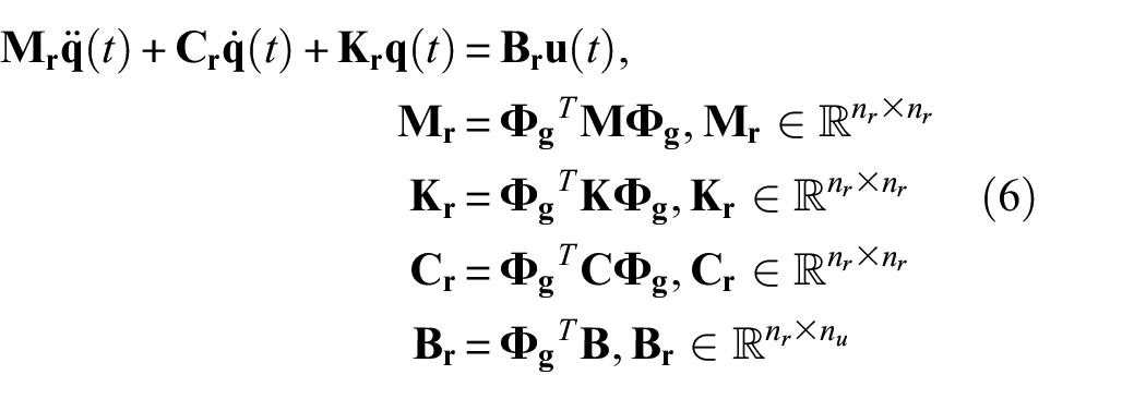
\bar{K} = [\begin{matrix} I^{4 \times 4} & - I^{4 \times 4} \\ - I^{4 \times 4} & I^{4 \times 4} \end{matrix}]

(4)

Here, $K_{el, C}$ is the coupled stiffness matrix between DoFs and $I^{4 \times 4}$ is the $4 \times 4$ identity matrix. When dealing with large FE models, a reduced order model is defined by projecting the full order model (FOM) on a subspace, with $q \in R^{n_{r}}$ the vector of reduced DoFs, such that $n_{r} < < n_{d}$ . The $z$ vector can be approximated as follows:

z \approx Φ_{g} q

(5)

where $Φ_{g} \in R^{n_{d} \times n_{r}}$ is a global reduction basis that spans the parameter space of interest.²⁶ By projecting Equation (2) onto the subspace spanned by $Φ_{g}$ , the following equations of motion for the reduced model are obtained:

\begin{matrix} M_{r} \overset{\cdot\cdot}{q} (t) + C_{r} \overset{\cdot}{q} (t) + K_{r} q (t) = B_{r} u (t), \\ M_{r} = {Φ_{g}}^{T} M Φ_{g}, M_{r} \in R^{n_{r} \times n_{r}} \\ K_{r} = {Φ_{g}}^{T} K Φ_{g}, K_{r} \in R^{n_{r} \times n_{r}} \\ C_{r} = {Φ_{g}}^{T} C Φ_{g}, C_{r} \in R^{n_{r} \times n_{r}} \\ B_{r} = {Φ_{g}}^{T} B, B_{r} \in R^{n_{r} \times n_{u}} \end{matrix}

(6)

where $M_{r} \in R^{n_{r} \times n_{r}}$ , $C_{r} \in R^{n_{r} \times n_{r}}$ , $K_{r} \in R^{n_{r} \times n_{r}}$ , $B_{r} \in R^{n_{r} \times n_{u}}$ are the reduced mass, damping, stiffness, and input matrices, respectively.

Reduction basis

This contribution employs the POD method to compute the reduction basis of the parametric Reduced Order Model (pROM). The main principle of the POD is to find a global reduction basis $Φ_{g}$ , spanning the full parameter subspace of interest, by selecting the meaningful shapes or modes of the solution provided by local reduction bases $Φ_{l}$ . In the specific case of DCB model (Figure 3), local bases are computed by solving the linear eigenvalue problem of the corresponding sub-system $l = 1, . . ., n$ laying on the $F - d$ curve. The number of samples is equal to the number of discretized elements in the interface. Each sample differs from the next one by removing progressively one spring element, such that

n_{s}^{l} = n_{s}^{l + 1} + n_{n}

(7)

where $n_{s}^{l}$ is the number of springs in the $l$ -th model and $n_{n}$ is the number of nodes along the width of the model.

The most common ways to compute $Φ_{g}$ are by interpolating or concatenating local POD bases $Φ_{l}$ obtained for each sample.²⁶ When the number of samples is limited, the concatenation approach is preferred. Given a set of $n$ concatenated local subspace bases, the singular value decomposition is computed in order to remove possible linear dependencies among all the subspaces, as follows:

U Σ W = [Φ_{1} Φ_{2} Φ_{3} \dots Φ_{n}]

(8)

where $U$ and $W$ are the left and right singular vectors, while $Σ$ is a diagonal matrix of singular values. The global reduction basis $Φ_{g}$ of the parametric system is identified by selecting the first $r$ -left singular vectors, such that the following minimization problem is reached:

\min ∥ z - Φ_{g} q ∥_{2}

(9)

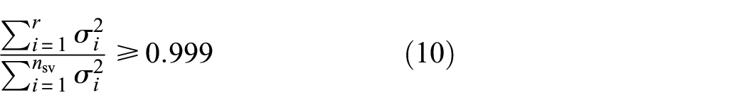
The number of selected values depends on the threshold criterion. A typical approach is to truncate the singular values such that²⁶

\frac{\sum_{i = 1}^{r} σ_{i}^{2}}{\sum_{i = 1}^{n_{sv}} σ_{i}^{2}} \geq 0.999

(10)

where $n_{sv}$ is the number of total singular values $σ_{i}$ .

Parameter estimation

The estimation of stiffness degradation in fracture process zone of the DCB model is here addressed by using the AEKF.^19,20,31

This choice is justified by the following rationale:

The augmented KF concurrently estimates the system states, external loads, and parameters. As part of its formulation, physical coupling is preserved and leveraged to obtain optimal estimates of the system states, external loads, and parameters. In general, this approach is also more computationally efficient and robust than for example, the dual KF.³²

The extended formulation, that is, extended Kalman filter (EKF), is an extension of KF for nonlinear or parametric systems by performing model linearization. Other formulations, for example, unscented Kalman filter,³¹ can be adopted when model linearization is not applicable. These approaches however do come at an increased computational cost, as they require the evaluation of so-called “sample points” per iteration step, whereas the EKF only requires a single evaluation per iteration step. Furthermore, constraint handling is typically more challenging, as the sampling approach has to be modified accordingly. Enforcing constraints within the EKF does not require these extensive modifications.

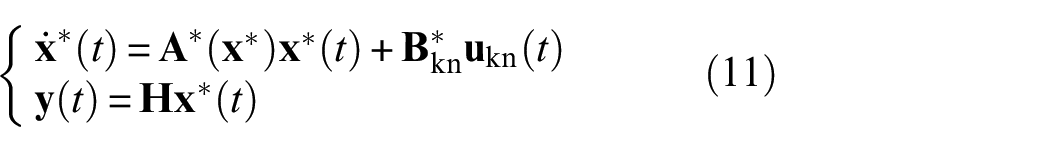
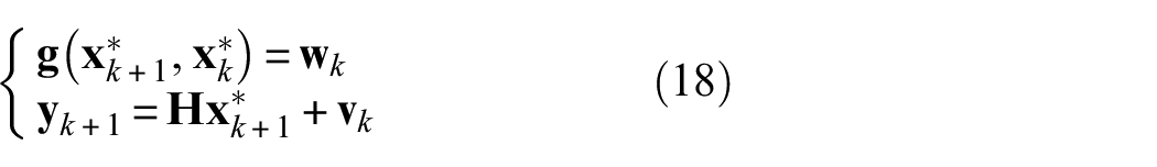
The AEKF scheme uses the dynamic system equations, that is, equations of motion, in a state-space formulation as follows:

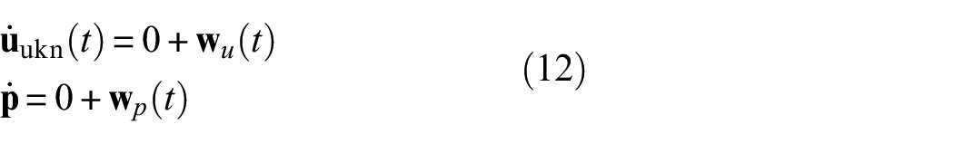
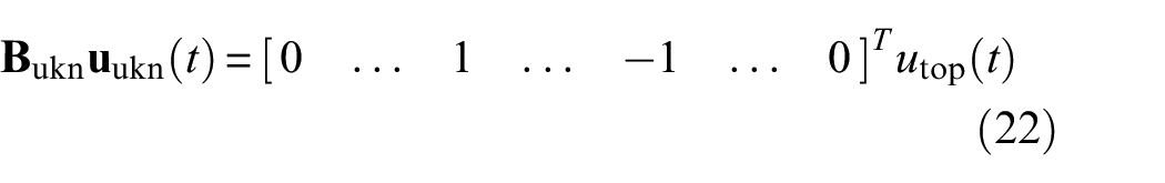
{\begin{matrix} {\overset{\cdot}{x}}^{*} (t) = A^{*} (x^{*}) x^{*} (t) + B_{kn}^{*} u_{kn} (t) \\ y (t) = H x^{*} (t) \end{matrix}

(11)

where $x^{*} (t)$ is the augmented state vector, that is, $x^{*} (t) = [q^{T} {\overset{\cdot}{q}}^{T} u_{ukn}^{T} p^{T}]^{T} \in R^{2 n_{r} + n_{u_{ukn}} + n_{p}}$ with $n_{u_{ukn}}$ and $n_{p}$ , respectively, the number of unknown loads and physical parameters to be estimated. The lattest is defined by the number of submodels included in the pROM. The vector of known input loads is denoted as $u_{kn}$ . The second equation in Equation (11) describes the measurement evolution in time $y (t)$ . The dynamic model of $u_{ukn}$ and $p$ has to be defined. Both quantities are described in this contribution as zeroth order random walk models^20,21,33:

\begin{matrix} {\overset{\cdot}{u}}_{ukn} (t) = 0 + w_{u} (t) \\ \overset{\cdot}{p} = 0 + w_{p} (t) \end{matrix}

(12)

where $w_{u}$ and $w_{p}$ are white Gaussian noise terms.

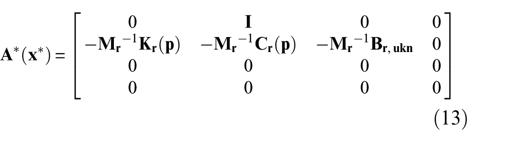
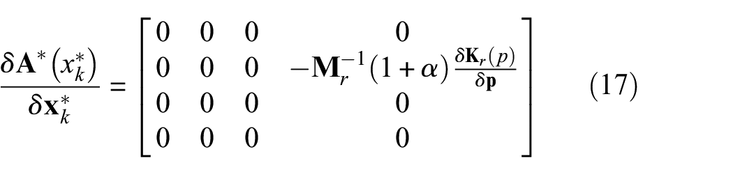
In Equation (11), the state matrix $A^{*}$ is function of the augmented state $x^{*}$ by defining a parametric dependency of the system. The parametric form of the $A^{*}$ with respect to parameter vector $p = [k_{s}^{l = 1 . . . n}]$ is defined as follows:

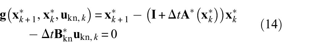
A^{*} (x^{*}) = [\begin{matrix} 0 & I & 0 & 0 \\ - {M_{r}}^{- 1} K_{r} (p) & - {M_{r}}^{- 1} C_{r} (p) & - {M_{r}}^{- 1} B_{r, ukn} & 0 \\ 0 & 0 & 0 & 0 \\ 0 & 0 & 0 & 0 \end{matrix}]

(13)

where proportional damping is assumed, that is, $C_{r} (p) = α K_{r} (p)$ . The DCB model shows a nonlinear degradation behavior at the interface, thus the extended formulation of the KF should be employed. The EKF needs the system linearization to propagate the state error covariance. Considering a first order explicit Euler integrator scheme, the discretized form of the equations of motion becomes:

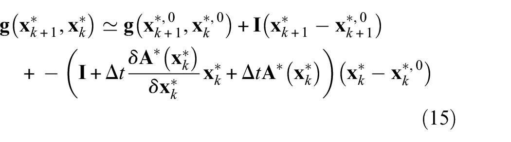
\begin{matrix} g (x_{k + 1}^{*}, x_{k}^{*}, u_{kn, k}) = x_{k + 1}^{*} - (I + Δ t A^{*} (x_{k}^{*})) x_{k}^{*} \\ - Δ t B_{kn}^{*} u_{kn, k} = 0 \end{matrix}

(14)

where $Δ t$ is the discrete time step. The linearization of Equation (14) around the states $x_{k + 1}^{*, 0}$ , $x_{k}^{*, 0}$ , truncated at the first order with Taylor expansion is

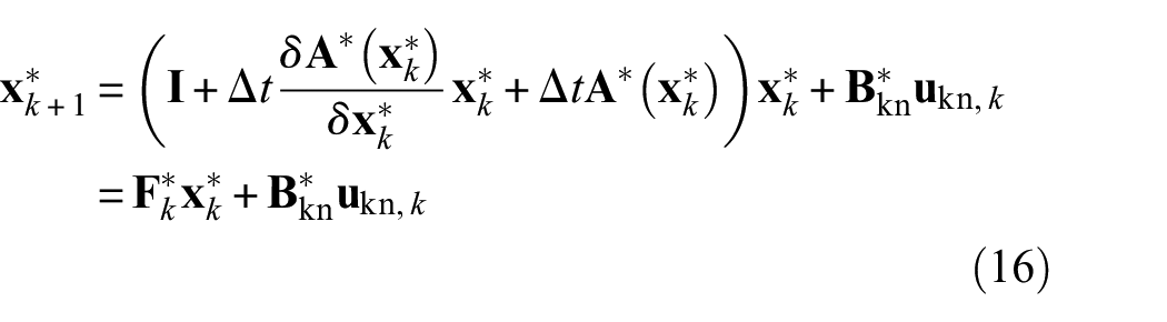
\begin{matrix} g (x_{k + 1}^{*}, x_{k}^{*}) \approx g (x_{k + 1}^{*, 0}, x_{k}^{*, 0}) + I (x_{k + 1}^{*} - x_{k + 1}^{*, 0}) \\ + - (I + Δ t \frac{δ A^{*} (x_{k}^{*})}{δ x_{k}^{*}} x_{k}^{*} + Δ t A^{*} (x_{k}^{*})) (x_{k}^{*} - x_{k}^{*, 0}) \end{matrix}

(15)

Resulting in:

\begin{matrix} x_{k + 1}^{*} = (I + Δ t \frac{δ A^{*} (x_{k}^{*})}{δ x_{k}^{*}} x_{k}^{*} + Δ t A^{*} (x_{k}^{*})) x_{k}^{*} + B_{kn}^{*} u_{kn, k} \\ = F_{k}^{*} x_{k}^{*} + B_{kn}^{*} u_{kn, k} \end{matrix}

(16)

where

\frac{δ A^{*} (x_{k}^{*})}{δ x_{k}^{*}} = [\begin{matrix} 0 & 0 & 0 & 0 \\ 0 & 0 & 0 & - M_{r}^{- 1} (1 + α) \frac{δ K_{r} (p)}{δ p} \\ 0 & 0 & 0 & 0 \\ 0 & 0 & 0 & 0 \end{matrix}]

(17)

Finally, the time-discrete formulation of the equations of motion is

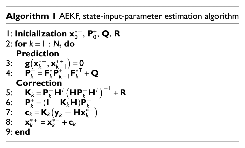
{\begin{matrix} g (x_{k + 1}^{*}, x_{k}^{*}) = w_{k} \\ y_{k + 1} = {Hx}_{k + 1}^{*} + v_{k} \end{matrix}

(18)

Vectors $w$ and $v$ are mutually uncorrelated Gaussian variables, and represent process and measurement noise, respectively. They are included in the equations of motion to take into account model and measurement uncertainties with the associated covariance matrices $Q$ and $R$ , respectively. Both covariance matrices are diagonal and their values drive the estimation performances.^18,20 Within this work, the highest uncertainty is attributed to the parameters $p$ and the unknown loads $u_{ukn}$ . The AEKF for joint state-input-parameter estimation is explained in Algorithm 1, where $x_{k}^{* -}$ is the a-priori state estimation at time step $k$ which is obtained from the numerical model of the system, $F^{*}$ is the transition matrix of Equation (16), $K_{k}$ is the Kalman gain, $c_{k}$ is the correction step, and $P_{k}^{-}$ , $P_{k}^{+}$ are the prior and posterior state covariance.

Algorithm 1 AEKF, state-input-parameter estimation algorithm

1: Initialization

x_{0}^{* -}

P_{0}^{+}

Q

R

2: for

k = 1 : N_{t}

do
Prediction
3:

g (x_{k}^{* -}, x_{k - 1}^{* +}) = 0

P_{k}^{-} = F_{k}^{*} P_{k - 1}^{+} F_{k}^{* T} + Q

Correction
5:

K_{k} = P_{k}^{-} H^{T} {({HP}_{k}^{-} H^{T})}^{- 1} + R

P_{k}^{+} = (I - K_{k} H) P_{k}^{-}

c_{k} = K_{k} (y_{k} - {Hx}_{k}^{* -})

x_{k}^{* +} = x_{k}^{* -} + c_{k}

9: end

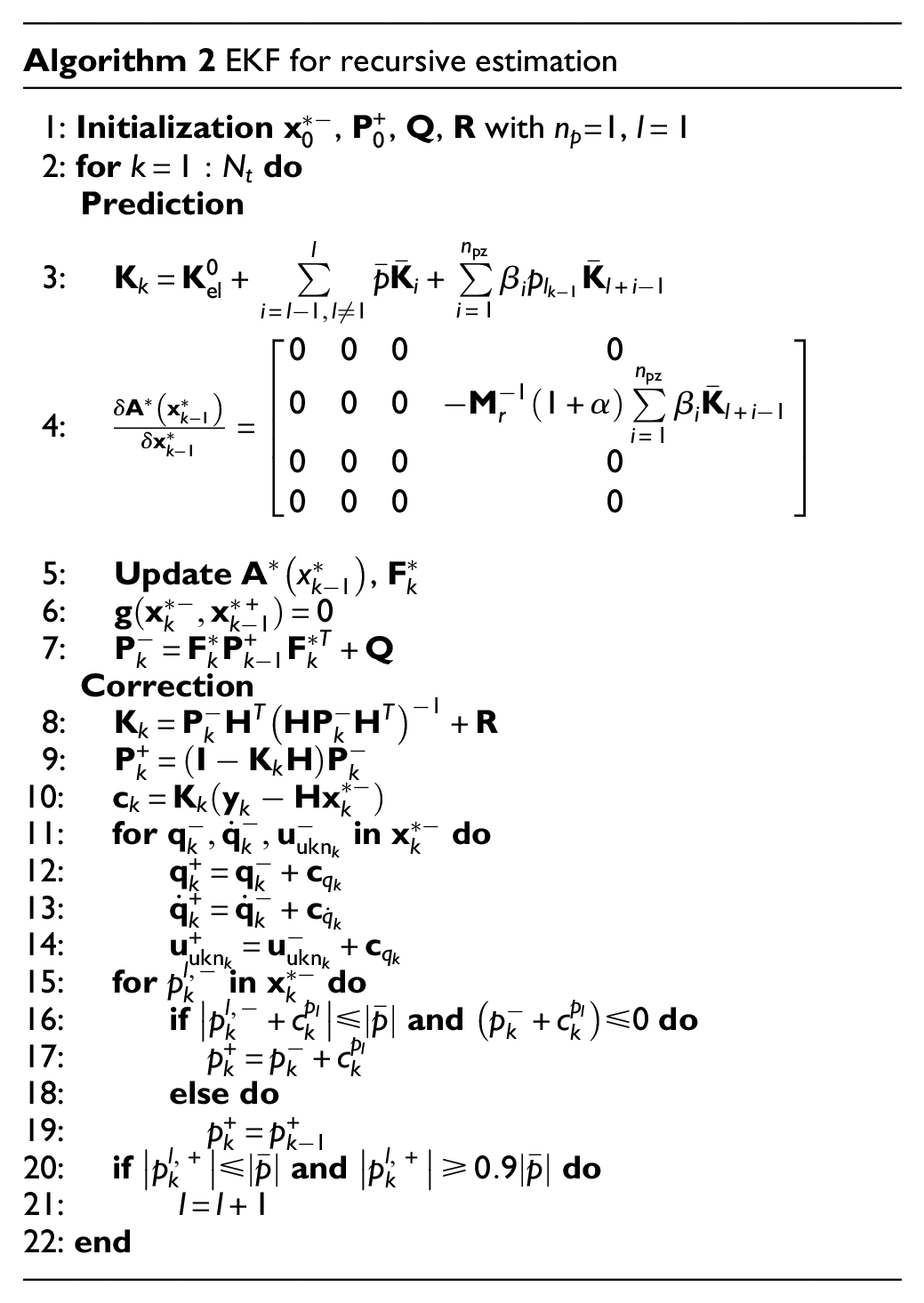
A modified version of the AEKF is proposed in this contribution with Algorithm 2 for delamination growth monitoring, by including

A correction step with constrained parameter values;

Recursive estimation assuming embedded distribution of parameter values.

Algorithm 2 EKF for recursive estimation

1: Initialization

x_{0}^{* -}

P_{0}^{+}

Q

R

with

n_{p} = 1

l = 1

2: for

k = 1 : N_{t}

do
Prediction
3:

K_{k} = K_{el}^{0} + \sum_{i = l - 1, l \neq 1}^{l} \bar{p} {\bar{K}}_{i} + \sum_{i = 1}^{n_{pz}} β_{i} p_{l_{k - 1}} {\bar{K}}_{l + i - 1}

\frac{δ A^{*} (x_{k - 1}^{*})}{δ x_{k - 1}^{*}} = [\begin{matrix} 0 & 0 & 0 & 0 \\ 0 & 0 & 0 & - M_{r}^{- 1} (1 + α) \sum_{i = 1}^{n_{pz}} β_{i} {\bar{K}}_{l + i - 1} \\ 0 & 0 & 0 & 0 \\ 0 & 0 & 0 & 0 \end{matrix}]

5: Update

A^{*} (x_{k - 1}^{*})

F_{k}^{*}

g (x_{k}^{* -}, x_{k - 1}^{* +}) = 0

P_{k}^{-} = F_{k}^{*} P_{k - 1}^{+} F_{k}^{* T} + Q

Correction
8:

K_{k} = P_{k}^{-} H^{T} {({HP}_{k}^{-} H^{T})}^{- 1} + R

P_{k}^{+} = (I - K_{k} H) P_{k}^{-}

10:

c_{k} = K_{k} (y_{k} - H x_{k}^{* -})

11: for

q_{k}^{-}, {\overset{\cdot}{q}}_{k}^{-}, u_{uk n_{k}}^{-}

x_{k}^{* -}

do
12:

q_{k}^{+} = q_{k}^{-} + c_{q_{k}}

13:

{\overset{\cdot}{q}}_{k}^{+} = {\overset{\cdot}{q}}_{k}^{-} + c_{{\overset{\cdot}{q}}_{k}}

14:

u_{uk n_{k}}^{+} = u_{uk n_{k}}^{-} + c_{q_{k}}

15: for

p_{k}^{l, -}

x_{k}^{* -}

do
16: if

| p_{k}^{l, -} + c_{k}^{p_{l}} | \leq | \bar{p} |

and

(p_{k}^{-} + c_{k}^{p_{l}}) \leq 0

do
17:

p_{k}^{+} = p_{k}^{-} + c_{k}^{p_{l}}

18: else do
19:

p_{k}^{+} = p_{k - 1}^{+}

20: if

| p_{k}^{l, +} | \leq | \bar{p} |

and

| p_{k}^{l, +} | \geq 0.9 | \bar{p} |

do
21:

l = l + 1

22: end

These two points are further explained in the following sections.

Modelling limitations in the correction term

The delamination growth monitoring consists of the estimation of stiffness degradation at the interface. The FE model of the DCB is initialized with very high stiffness $p_{0} = k_{s}$ values associated with the interface spring elements (Figure 3). During the estimation, each element $p^{l}$ of the stiffness parameter vector $p$ is constrained within the correction steps as follows:

$| p_{k}^{l, -} + c_{k}^{p^{l}} | \leq | \bar{p} |$ : at each time step, the predicted parameter value should not exceed the threshold parameter $\bar{p} = - p_{0}$ value imposed by the baseline FE model

$(p_{k}^{l, -} + c_{k}^{p^{l}}) \leq 0$ : the estimation always returns stiffness degradation. This means that a negative value is always added to the system. A positive value would mean an increase of stiffness with respect to the baseline model, which is a nonphysical solution.

Recursive parameter estimation

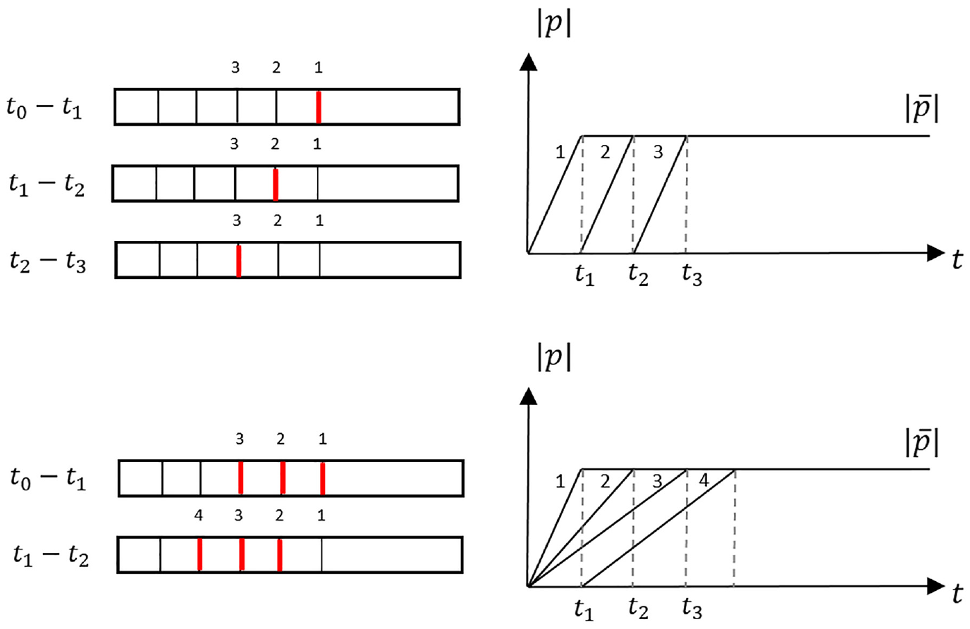
The number of parameters $n_{p}$ estimated for a DCB model is equal to the number of elements modeled at the interface. The simultaneous estimation of a high number of states is computationally expensive and requires a high number of sensors to fulfill the system observability requirements.^18,21,34 For this reason, a recursive estimation approach is proposed in this contribution which effectively relaxes, and therefore reduces, the required number of sensors. This means that the model parametrization itself is dynamic: depending on the crack propagation, a different set of interface stiffness elements is updated. At time step $k = 0$ , only $p^{l = 1}$ is estimated. Once $p^{l = 1}$ reaches the threshold value $\bar{p}$ , the stiffness matrix is updated. At a generic time step $k$ :

K (p_{k}) = K (p_{k}^{l = i}, p_{k}^{l = [1 : i - 1]} = \bar{p}, p_{k}^{l = i + 1, . . n_{s}} = p_{0})

(19)

When the $l$ -th elemental interface stiffness is zero, that is, $p_{k}^{l} = p_{0} + \bar{p}$ , the delamination is propagating.

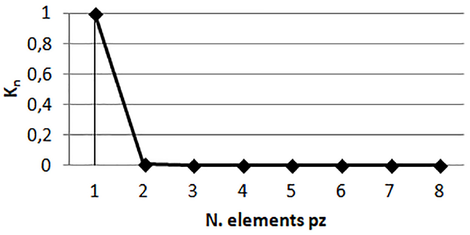
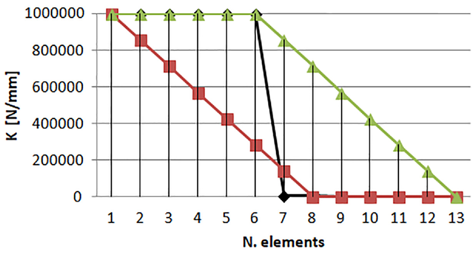
This recursive approach assumes that the stiffness degradation in each spring element occurs gradually as a ramp function (Figure 5) until reaching the target value. The velocity at which the elements are degrading is driven by the parametric dependency adopted in the estimation. This assumption does not allow stiffness distribution at the interface, that is the case for materials with very low fracture toughness $G_{IC}$ . In a more generic condition, the delamination involves a process zone with its stiffness distribution. To guarantee a more physical workflow, a distribution function is thus proposed among the $n_{pz}$ elements modeled in the process zone length. By considering the $l$ -th element $p^{l} = p^{m}$ , that is, the master parameter, and the vector of parameters $p_{pz} \in R^{n_{pz}}$ along the beam span, the following relation exists:

p_{pz} = B_{p} p^{m}

(20)

Figure 5.

Recursive parameter estimation without (top) and with (bottom) distribution.

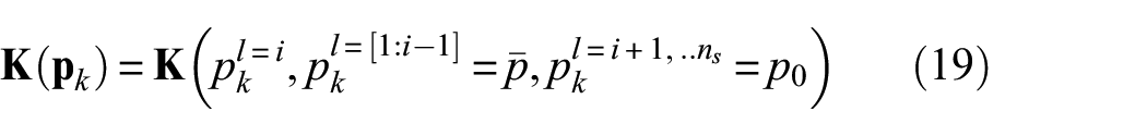
where $B_{p} \in R^{n_{pz}}$ is a vector with weight coefficients $β^{l}$ , which allows to distribute the master parameter value to the slave nodes in the process zone. Figure 5 shows an example of estimation by considering a recursive distributed estimation over $n_{pz} = 3$ elements. The estimation is still recursive on the master parameter, but the estimated value is distributed over the next $n_{pz}$ parameters via the weights. Line $20$ of Algorithm 2 indicates that the switch from $l$ -th to $(l + 1)$ -th parameter is possible when $| p^{l} |$ falls in the range $[0.9 - 1] \bar{p}$ . The lower limit could require tuning, because it could happen that the filter will not reach a “perfect” estimated value, that is, $| p_{k}^{l, +} | = | \bar{p} |$ .

System observability

One of the requirements of the KF estimation is to have a set of measurements which guarantees the observability of the system. Extensive explanation has been presented in²⁰ for parametric systems. Considering only position-level measurements and the stiffness parametrization of Equation (3), the following major conclusions are summarized here:

Stiffness parameters cannot be estimated in a static condition if no known loads are applied.

The system is unobservable in static conditions as well for the joint, that is, concurrent, parameter and input estimation if no known loads are applied.

These considerations are further addressed in the numerical/experimental validation sections below.

Estimation of delamination growth in a DCB model: numerical validation

A numerical validation is presented in this section in order to validate the proposed recursive parameter estimation approach. In particular, the following studies are addressed:

Performances of crack propagation estimation via AEKF parameter and joint parameter/input schemes with respect to the number of measurements.

Effect of prior knowledge of process zone length included in the distributed estimation of parameters.

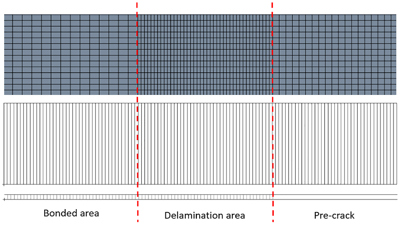
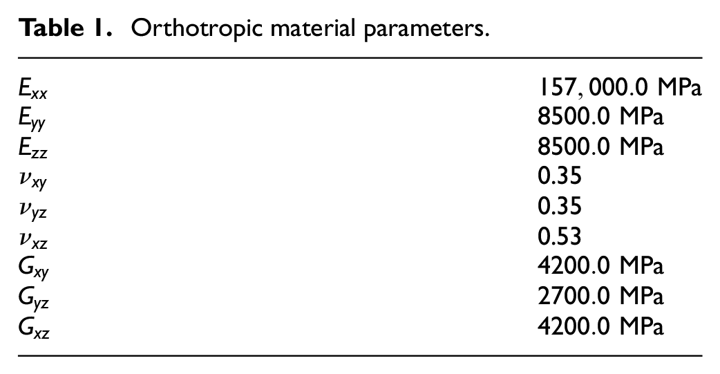
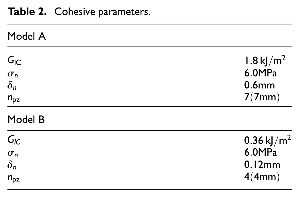
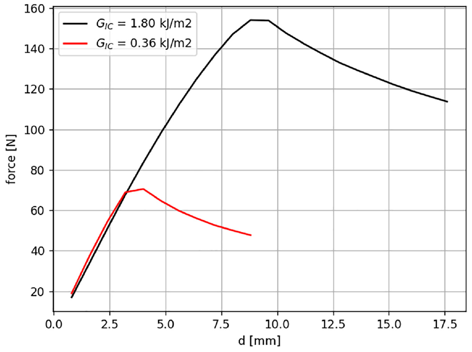
Two DCB models are considered: the nonlinear FE model for reference simulated data and its linear counterpart (Figure 6). Both models are 25 mm wide, 120 mm long, 3 mm thick and the pre-crack length is 38 mm. The two arms are zero degree unidirectional laminates whose material properties are summarized in Table 1. Two sets of cohesive properties have been considered and are listed in Table 2. The lower value of Mode I interlaminar fracture toughness $G_{IC}$ is representative of a brittle interface that promotes a quick crack propagation with limited process zone. Contrarily, a high $G_{IC}$ value means that high loading is required to propagate damage and a longer process zone is involved. The different process zone lengths resulting from the nonlinear analysis are used to identify the number of physical parameters involved in the distributed estimation.

Figure 6.

Nonlinear (top) and linear (bottom) meshes with node-to-node spring interface.

Table 1.

Orthotropic material parameters.

$E_{xx}$	$157, 000.0$ MPa
$E_{yy}$	$8500.0$ MPa
$E_{zz}$	$8500.0$ MPa
$ν_{xy}$	0.35
$ν_{yz}$	0.35
$ν_{xz}$	0.53
$G_{xy}$	$4200.0$ MPa
$G_{yz}$	$2700.0$ MPa
$G_{xz}$	$4200.0$ MPa

Table 2.

Cohesive parameters.

Model A
$G_{IC}$	$1.8 kJ / m^{2}$
$σ_{n}$	$6.0 MPa$
$δ_{n}$	$0.6 mm$
$n_{pz}$	$7 (7 mm)$
Model B
$G_{IC}$	$0.36 kJ / m^{2}$
$σ_{n}$	$6.0 MPa$
$δ_{n}$	$0.12 mm$
$n_{pz}$	$4 (4 mm)$

The nonlinear model consists of hexahedral elements, connected with zero-thickness interface cohesive elements. The minimum cohesive element length is 1 mm. The bi-linear cohesive law is defined at the interface. The model is solved using an implicit integrator. The obtained reaction force versus opening displacement is shown in Figure 7 for the two cohesive models.

Figure 7.

Force versus displacement curve for the two values of $G_{IC}$ .

The linear model employed in the KF scheme (Figure 6) consists of shell elements. The spanwise mesh size is 1 mm, in accordance with the element length in the delamination area used in the nonlinear simulation. The two beams are connected through node-to-node spring elements connecting the $z$ DoFs, as shown in Figure 4. The number of DoFs in the linear model is $n_{d} = 2880$ . Despite the advantages of using a simplified FE model with shell elements, some modelling issues could arise:

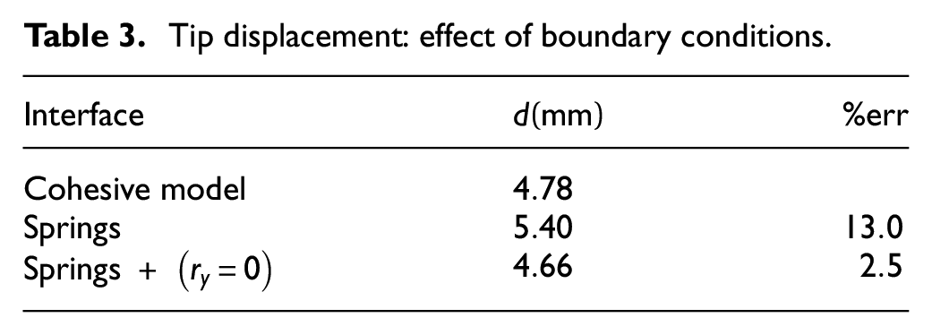
Boundary conditions at the crack tip: the two arms ahead the crack can deform in the axial direction and allow small rotations. Shell elements do not capture this effect, which is however allowed in a FE model that has been meshed through the thickness, that is, beam cross section. The effect of boundary conditions has been presented in³⁵ where different nodal constraints are investigated. The model with shell elements connected with node-to-node springs results to be the most accurate to predict delamination and it is considered in this work for the computation of the pROM.

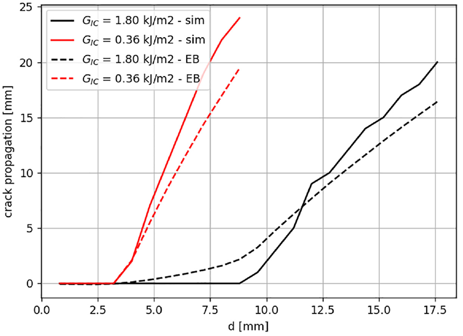
Rotational bending effects and shear deformations: in Skec et al.,³⁷ the delamination growth in a DCB specimen has been investigated analytically with Euler Bernoulli (EB) and Timoshenko theories. The work highlights that a loss of accuracy is observed for brittle materials if no rotational bending effects and shear deformations are considered. The employed model takes into account these effects.

Figure 10 shows the crack propagation for model A and model B and compares the data obtained from the nonlinear simulation with data retrieved from the EB theory for each pair of force—displacement values. The comparison shows that the EB theory diverges from the nonlinear curve when the linear behavior is not followed anymore (Figure 7) and underestimates the final crack length value of $20 %$ . This effect appears earlier during the simulation for model A since a longer process zone is involved and thus the boundary conditions at the crack tip have a greater impact on the bending arm behavior. A static analysis has been performed by applying the maximum reaction force on the linear shell model in the following situations (Figure 8):

Node-to-node springs applied at the interface elements connecting the $z$ -direction. The interface stiffness distribution in the process zone resulting from the nonlinear simulation with cohesive elements has been applied (Figure 9).

Constrained $r_{y}$ DoF, that is, bending, of first undamaged nodes (point B in the Figure 3) at the interface, in addition to conditions specified in the previous point.

Figure 8.

Interface stiffness law in the process zone. $K_{n}$ normalized spring stiffness.

Figure 9.

Normalized stiffness distribution in the process zone of the nonlinear model with cohesive elements.

Table 3 compares the tip displacement of the upper arm obtained with the different boundary conditions. The node-to-node spring model without any local rotational constraints results to be more flexible, as also validated in.³⁵ Constraining $r_{y}$ DoF would require more laborious modelling during estimation. Indeed, a recursive approach regarding the constraints of the undamaged nodes should be elaborated, considering that those nodes change during delamination propagation. For this reason, a simpler model, that is, node-to-node springs, is considered in this contribution and the effect of modelling errors on the estimation are further investigated.

Table 3.

Tip displacement: effect of boundary conditions.

Interface	$d (mm)$	$% err$
Cohesive model	$4.78$
Springs	$5.40$	$13.0$
Springs + $(r_{y} = 0)$	$4.66$	$2.5$

Parameter space

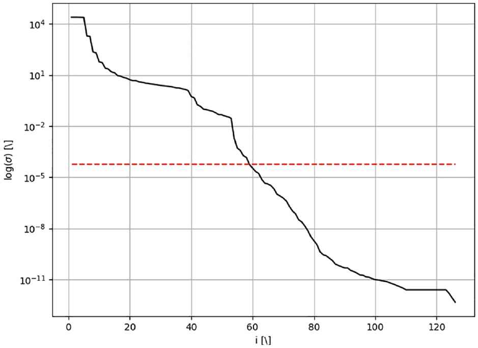
As explained in section “Reduction basis,” the parametric space characterized by a set of linear models, by means of sequentially removing a sectional spring. The number of models to be included in the pROM scheme is defined by the crack propagation length in the nonlinear simulation analysis (Figure 10). A total of $n = 25$ models is chosen. For each model, the local reduction basis is defined by the first bending mode and 4 static modes, that is, residual attachment modes.³⁷ These modes allow to have an exact representation of the static response of the structure for a given input location. In this case, each of the static modes corresponds to the vertical DoF of the 4 nodes at the tip of the two arms, where the forces are applied to pull both arms. Only 1 normal mode is considered as only quasi-static analyses are investigated in this work. For fatigue analysis, more normal modes should be considered within the frequency range of interest. Ideally, a more refined study on the parametric space should be performed by sampling the local distribution at the interface as in Figure 5. However, this study is out of the scope of this work and the chosen parameter samples are considered adequate to allow sufficient accuracy of the interpolation over the full parameter space. The SVs of the concatenated basis are shown in Figure 11 as well as the adopted threshold value. The final global reduction basis has dimension $r = 59$ .

Figure 10.

Crack propagation of model A and model B. Comparison between simulated curves and data retrieved from EB theory.

Figure 11.

Singular value decomposition of parametric concatenated basis. Red line: threshold value.

Results

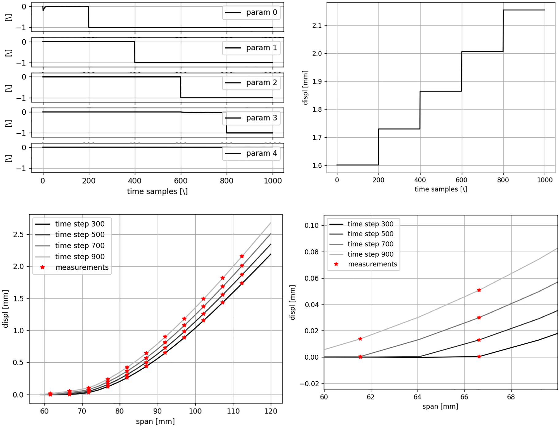
The current section aims to validate the recursive estimation algorithm for crack growth monitoring in composite materials. As a first step, displacement sensor data have been generated from the linear FE model by applying constant pull-forces at the tip of the two arms and artificially removing 3 springs at the interface after a fixed time window. The results of the estimation are shown in Figure 12 with $n_{pz} = 3$ and $B_{pz} = [111]^{T}$ . Furthermore, 22 displacement measurements are considered, equally distributed between the top and bottom laminae. The results show a perfect estimation of the parameter degradation and reconstruction of displacement field, which therefore appears to validate the proposed recursive estimation approach. Good levels of accuracy are also obtained locally at the boundary conditions of the beam after sequential removal of springs. In the following, the estimation results on the two DCB models with interface properties in Table 2 are shown.

Figure 12.

Estimated parameters (top left), samples of measurements (top right), estimated displacement field distribution at different time samples (bottom left) and corresponding estimation of boundary conditions (bottom right).

Sensors networks

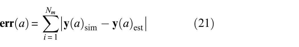
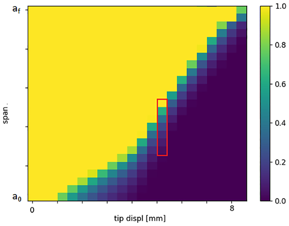
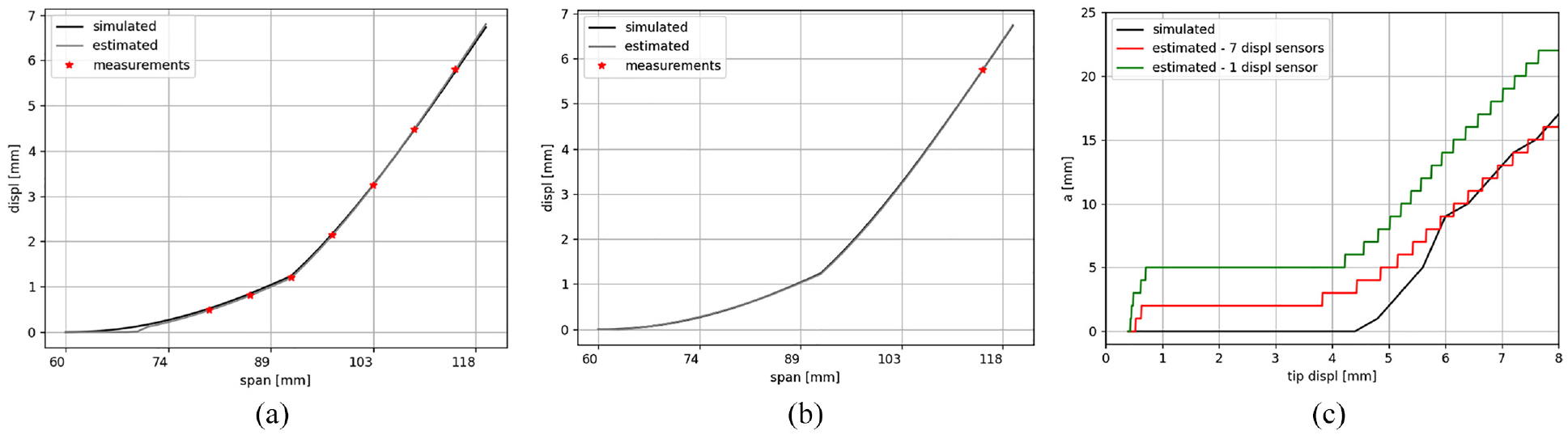
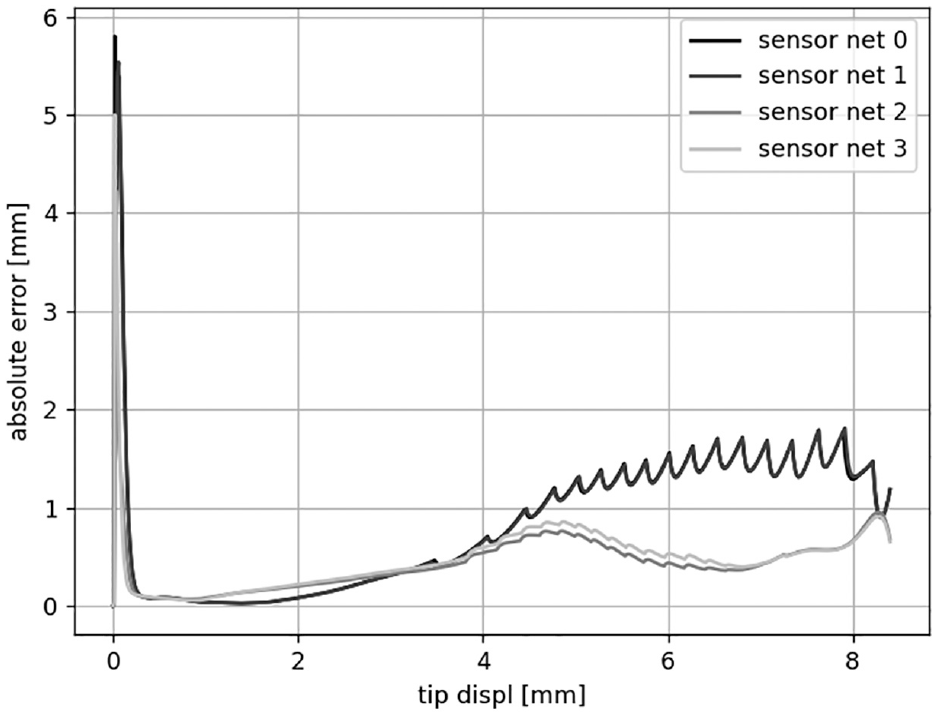
A brief study about the optimal sensor network is proposed in this section to guarantee the system observability as described in section “System observability.” Model $A$ is considered in this section, but the obtained results also be generalized to model $B$ . The loads are assumed to be known, thus the reaction forces obtained by the nonlinear DCB simulation are applied to the linear model. The parameter $n_{pz}$ has been fixed equal to the number of elements in the process zone of the nonlinear analysis (Table 2). Figure 13 shows the interface stiffness, that is, ${\bar{K}}_{c} = (1 - D) K_{c} = τ / δ$ , in the span-wise direction. The process zone of model A involves approximately 7 mesh elements, thus $n_{pz} = 7$ , and a linear distribution of parameters is assumed. Different sensor networks have been tested within this section. The scope is to start from a distributed map of sensors, equally spaced along the span of the top arm and symmetrically applied to the bottom one, and to gradually remove some sensors to evaluate the resulting loss of accuracy. The considered number of displacement sensors on the top lamina are $14$ , $7$ , and $3$ , distributed between 0.6 and 1.0 $L$ , starting from the root of the arms. Another analysis has been performed by considering only a tip displacement sensor on the top and bottom arms. Figure 14 shows the crack length estimation and the shape reconstruction corresponding to a generic crack $a$ greater than the critical value $a_{c}$ . Figure 15 shows the estimation error on the displacement field computed as:

err (a) = \sum_{i = 1}^{N_{m}} | y {(a)}_{sim} - y {(a)}_{est} |

(21)

Figure 13.

Normalized stiffness at each time step in the delaminated area. The span is from the initial delamination $a_{0} = 38 mm$ to $a_{f}$ , that is, delamination at the end of the simulation. The red box indicates a generic evaluation of process zone.

Figure 14.

Shape reconstruction and crack length estimation on model A with different sensor networks. (a) Seven displacement sensors on the top lamina. $a > a_{c}$ , (b) one displacement sensors on the top lamina. $a > a_{c}$ , (c) estimated crack length. $n_{pz} = 7$ .

Figure 15.

Absolute error of the simulated versus measured vertical displacements of model A, known loads. Sensor net 0, 1, 2, 3 correspond to 14, 7, 3, 1 measurements on the top lamina employed in the estimator respectively.

where $y {(a)}_{sim} \in R^{N_{m}}$ and $y {(a)}_{est} \in R^{N_{m}}$ are the full-field $N_{m}$ simulated and estimated displacements in vertical direction. The estimated crack starts to propagate earlier compared to what is expected from the EB solution in Figure 10. This can be partially explained by the initial noise on the estimation process as well as the modelling errors, that is, lack of rotational constraints in the translational $z -$ DoF springs and linear stiffness distribution assumed at the interface. As discussed in previous works,^18–20 the estimator compensates here for the modelling errors in order to match the measurements. This error compensation can be explained by looking at the crack length obtained with 1 sensor: once the model reaches the critical reaction force, the stiffness distributions in the process zone of the reference and the linear models are as shown in Figure 14. The reference model is shown to be much more flexible as the stiffness within the process zone is very low when compared to the assumed linear distribution where the crack tip is assumed to be at the same element. Thus, the filter estimates the same trend of crack propagation of the reference model but with a crack tip shifted toward the root, in order to match the measured tip displacement. Even if the stiffness in the first element of the estimated process zone, that is, $n = 7$ in Figure 16, is lower than the limit value assumed in the model, that is, $K = 10^{6} N / mm$ , its value is still sufficiently high to converge to a quasi-fixed boundary condition on the translational DoF. The reason why the estimation with 7 sensors returns lower accuracy is because the estimator is constrained to behave more similarly to the inverse solution of EB theory, as shown in Figure 10, as it needs to match more distributed measurements. Indeed, the trend is the same as observed in Figure 10, but shifted by about 3 mm. The effect of a different stiffness distribution law in the process zone is quantified for the joint input/parameter estimation case by comparing the linear distribution with the one shown in Figure 9.

Figure 16.

Stiffness distribution: cohesive law (black, pz: 7–13) versus estimated linear (red, pz: 1–8) versus expected linear (green, pz: 6–13).

Unknown loads: joint input/parameter estimation

The analyses performed so far consider the external loads to be known. The critical loads leading damage propagation are often unmeasurable during operation. The joint input/parameter estimation is tested here on the DCB model using the proposed recursive approach. Given the symmetry of the model, a single load is estimated and equally, that is, symmetrically, distributed between top and bottom laminae as follows:

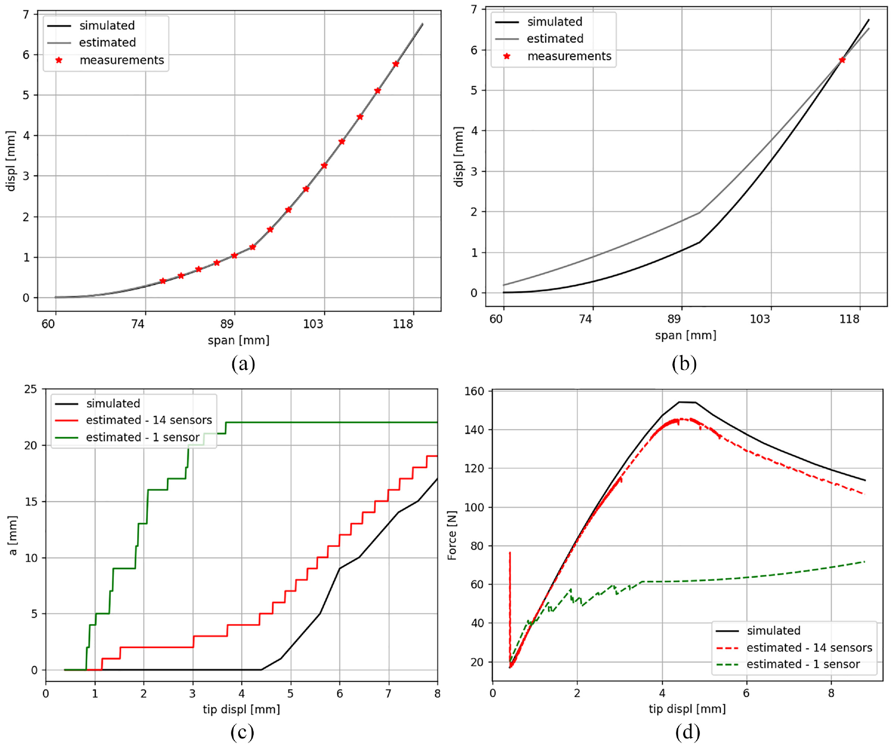
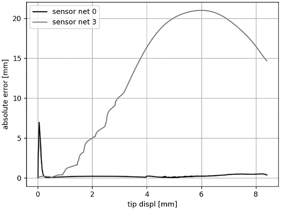
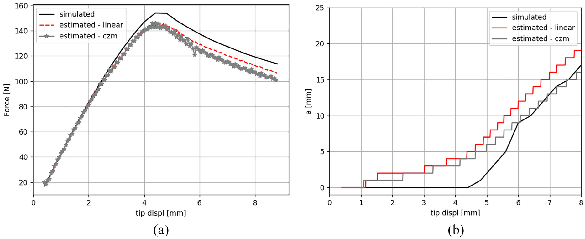
B_{ukn} u_{ukn} (t) = {[\begin{matrix} 0 & \dots & 1 & \dots & - 1 & \dots & 0 \end{matrix}]}^{T} u_{top} (t)

(22)

where $u_{top} (t)$ is the estimated load. $B_{ukn}$ is a vector with nonzero elements at the vertical DoFs of the two tip nodes, where the loads are applied. A constant load with low amplitude of $1 N$ is also applied during the estimation in order to guarantee system observability as explained in the dedicated section. Figure 17 shows the estimation of reaction force, crack propagation and shape reconstruction while Figure 18 show the estimation error on displacement data obtained on model A, with $14$ and $1$ displacement sensors on the top lamina and $n_{pz} = 7$ . The crack length starts to propagate earlier and the estimated force diverges from the reference values in agreement with the simplified model behavior (Figure 10). As in McElroy,³⁵ the reaction force is under estimated by approximately $6 %$ when the damage propagates. Similar behavior can be observed for model B (Figure 19) with $14$ displacement sensors and $n_{pz} = 4$ .

Figure 17.

Joint input/parameter estimation results using model A. $n_{pz} = 7$ . (a) Fourteen displacement sensors on the top lamina. Shape reconstruction at $a > a_{c}$ , (b) one displacement sensor on the top lamina. Shape reconstruction at $a > a_{c}$ , (c) estimated crack length, and (d) estimated reaction force.

Figure 18.

Absolute error of the simulated versus measured vertical displacements of model A, unknown loads. Sensor net 0, 3 correspond to 14, 1 measurements on the top lamina employed in the estimator.

Figure 19.

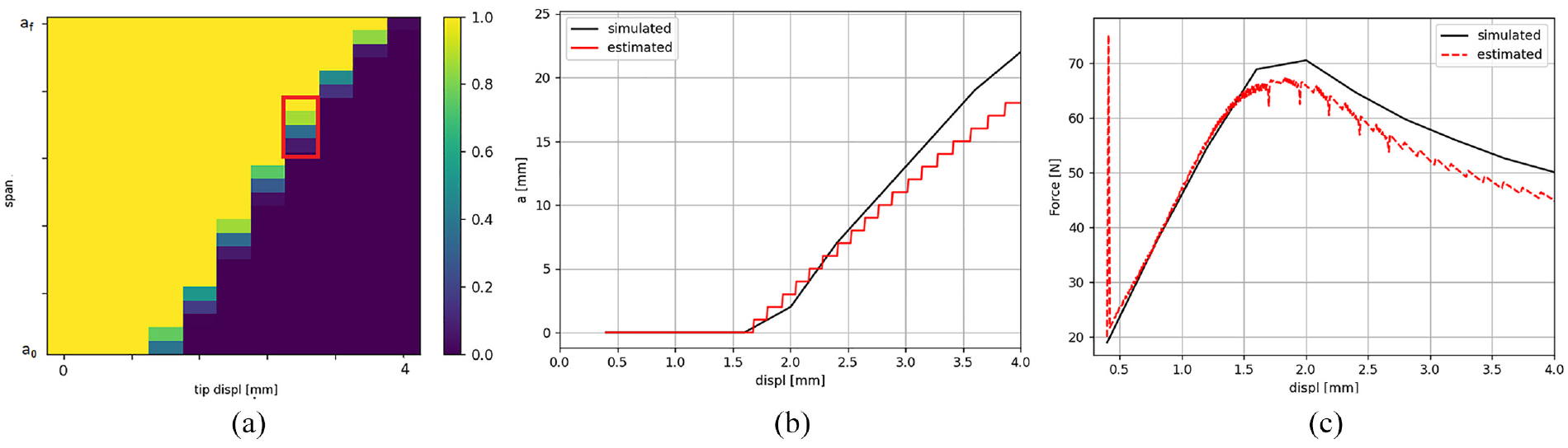
Joint input/parameter estimation results using model B. $n_{pz} = 4$ . (a) Normalized stiffness with process zone length (red box) from simulated model. (b) Estimated crack length—14 displacement sensors, (c) estimated reaction force—14 displacement sensors.

The following conclusions can be drawn on the joint input/parameter estimation of a DCB model:

When the load is unknown, the system parameters become unobservable if no collocated measurements are considered. Indeed a loss of accuracy is observed if only one tip measurement is used, because of lack of information regarding the interface behavior;

The critical load is under-estimated for both models, as well as the reaction force. This is caused by the boundary conditions, that is, modelling error, in the simplified model employed in the KF, which has unconstrained rotations at the crack tip. The estimation therefore compensates for these modelling errors, leading to a loss of accuracy of the estimated quantities, that is, parameters and loads. In this case, the loads exhibit a decreasing of accuracy because higher uncertainty has been assumed, that is, $Q_{u} > > Q_{p}$ .

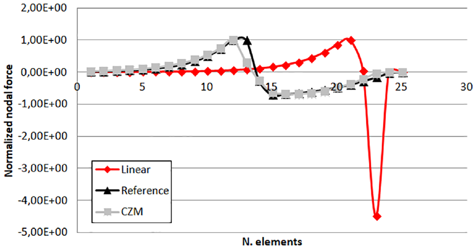
As further analysis, the effect of the imposed stiffness distribution in the process zone embedded in the AEKF scheme is shown in Figure 20. The linear and the reference cohesive distributions are tested for model A, by using $14$ displacement measurements on the top arm. The results do not add significant changes to the previous conclusions. Indeed, a different distribution leads to a different estimation of the crack propagation. The estimated reaction force obtained with the cohesive law results to be different from the one obtained with linear distribution because it compensates somehow for the different distribution of forces observed at the crack tip (Figure 21). As a main conclusion of this contribution, the crack propagation can thus be monitored with acceptable accuracy even when using a less-correlated numerical model, if loads and parameters are jointly estimated. Indeed, the modelling errors are compensated within the estimation, resulting in a lower force amplitude with $6 %$ of error.

Figure 20.

Joint input/parameter estimation results on model A. $n_{pz} = 7$ , 14 displacement sensors. Comparison between different imposed interface stiffness distributions. (a) Estimated reaction force and (b) estimated crack length.

Figure 21.

Normalized nodal forces at the interface with respect to the value at the first undamaged element. Linear and CZM are retrieved from the forward simulation using the linear shell model with imposed stiffness distributions in the process zone. CZM: cohesive zone model.

Experimental validation

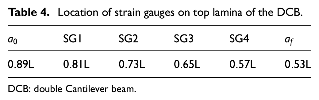
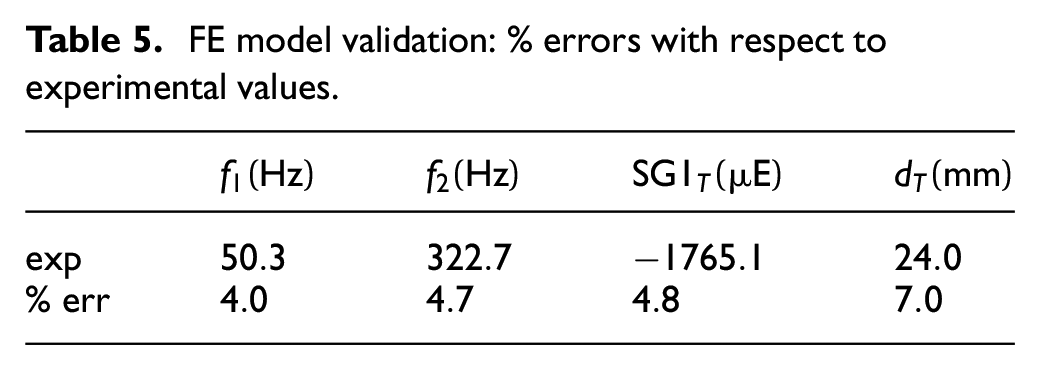
Within this section, the test case shown in Figure 2 is presented and the recursive estimation is validated using experimental strain data. In compliance with the EN 6033 standard,²⁷ a $L = 250 mm$ long and $w = 25 mm$ wide prismatic coupon with a thickness $t = 3.3 mm$ is extracted from a $[0, 90]_{4 s}$ woven laminate that presents on its mid-plane a teflon film such that the initial delamination is approximately $a_{0} = 26 mm$ . Plane hinges have been installed at the tip of the coupon on the teflon insert side to apply the mechanical load. Four strain gauges have been installed on the external layer of the coupon along its mid-line starting from $46 mm$ from the tip with a spacing of $20 mm$ . The elastic properties of the material are validated using both static data as well as a modal analysis. Figure 22 shows the setup of a cantilever beam with same stacking sequence and same geometry of the DCB specimen. The modal parameters have been acquired through impact modal analysis by installing 2 accelerometers as in Figure 22. The elastic parameters $E_{xx} = E_{yy}$ of the FE model have been tuned in order to match the first and second bending normal modes. The other elastic properties, coming from previous material calibration analysis are considered constant during model validation since their influence on bending modes is negligible (Data can be made available on request). The static response in terms of strains is also considered as target of the FE model optimization. In particular, the linear elastic DCB model is simulated for static analysis by applying the latest value of the measured reaction force and the corresponding strain values and tip displacement are compared. The location of sensors installed on the top lamina is reported in Table 4. Results of the FE model validation are shown in Table 5.

Figure 22.

Test setup for experimental modal analysis.

Table 4.

Location of strain gauges on top lamina of the DCB.

$a_{0}$	$SG 1$	$SG 2$	$SG 3$	$SG 4$	$a_{f}$
$0.89 L$	$0.81 L$	$0.73 L$	$0.65 L$	$0.57 L$	$0.53 L$

DCB: double Cantilever beam.

Table 5.

FE model validation: % errors with respect to experimental values.

	$f_{1} (Hz)$	$f_{2} (Hz)$	$SG 1_{T} (μ E)$	$d_{T} (mm)$
exp	$50.3$	$322.7$	$- 1765.1$	$24.0$
% err	$4.0$	$4.7$	$4.8$	$7.0$

Crack propagation

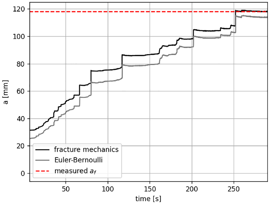
The crack length propagation has been retrieved from experimental data. From EB theory, the maximum deflection of a cantilever beam, that is, $δ = \frac{P a^{3}}{3 EI}$ , is first used, where $δ$ and $P$ are respectively the tip displacement and the reaction force. The crack length $a$ is shown in Figure 23: the last value is about $3.6$ % below the target, that is, last measured value during the test. An alternative approach is to retrieve $a$ from the mode I interlaminar fracture toughness^38,39 as follows:

G_{IC} = \frac{mP δ}{2 wa} \frac{F}{N}

(23)

Figure 23.

Crack propagation retrieved from experimental data.

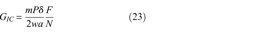
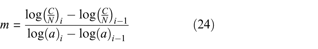
where $F$ and $N$ are correction factors taking into account the effects of large displacements and the stiffening of the specimen due to the loading hinges. The influence of these factors is however negligible for the DCB specimen investigated in this contribution. Furthermore, $m$ is a parameter obtained from the specimen compliance, that is, $C = δ / P$ , defined as⁴⁰:

m = \frac{\log {(\frac{C}{N})}_{i} - \log {(\frac{C}{N})}_{i - 1}}{\log {(a)}_{i} - \log {(a)}_{i - 1}}

(24)

where $i$ indicates the $i$ -th time sample. By solving Equation (23), the crack length $a$ can be retrieved. $G_{IC}$ should be considered function of $a$ as the energy increases with the crack propagation. Because of the lackof dataavailability, the value corresponding to the last measured crack length $a_{f} = 118 mm$ is used, that is, $G_{IC} = 0.692 kJ / m^{2}$ . Equation (23) is then solved by “back-propagating” $a_{f}$ and the trend of $a$ is shown in Figure 23. In contrast with the EB approach, this procedure tends to overestimate the initial crack length. This is due to the fact that the assumption of a constant $G_{IC}$ measured for a fully propagated crack causes implies an excess of fracture energy in the crack initiation region.

Results

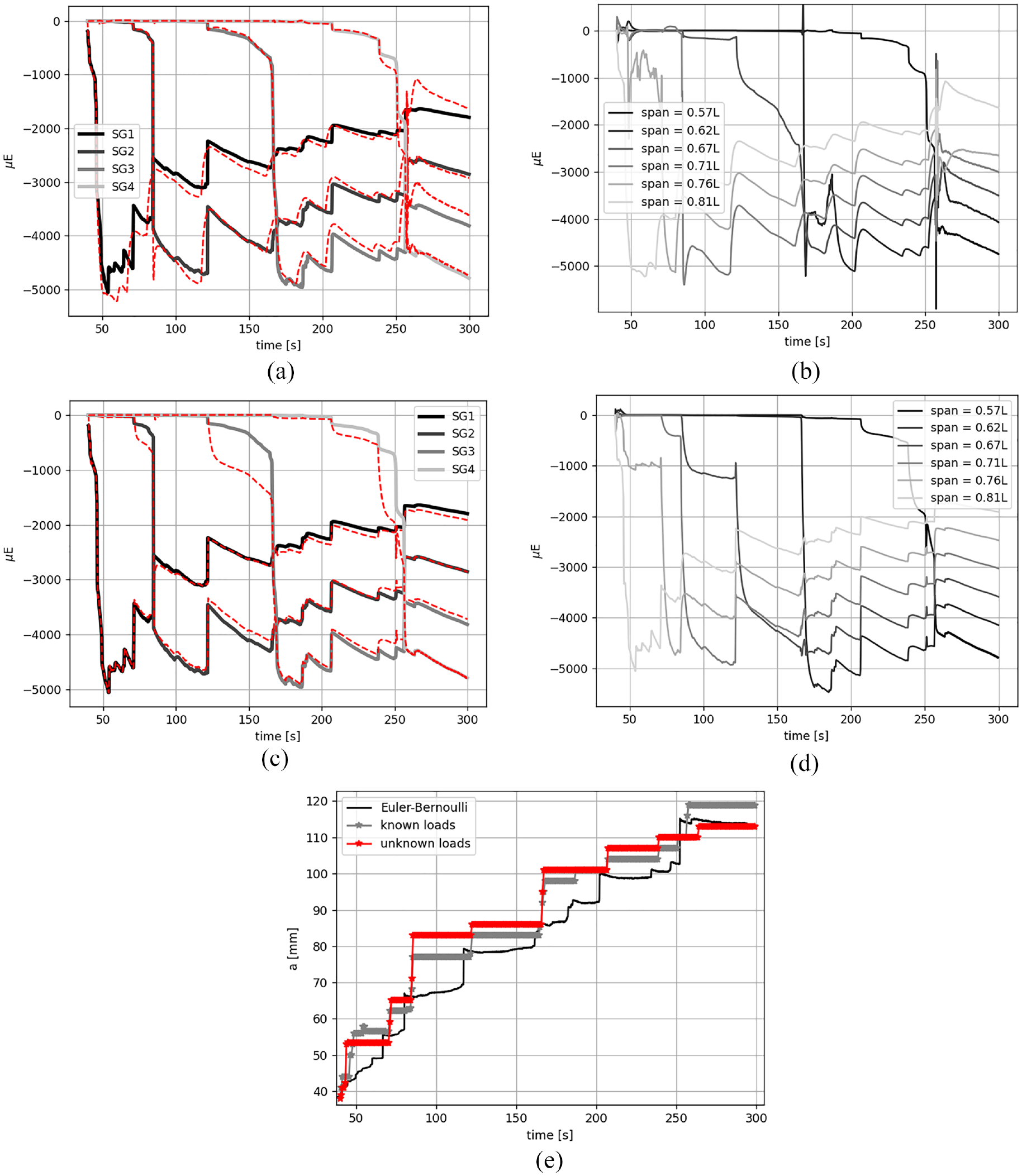
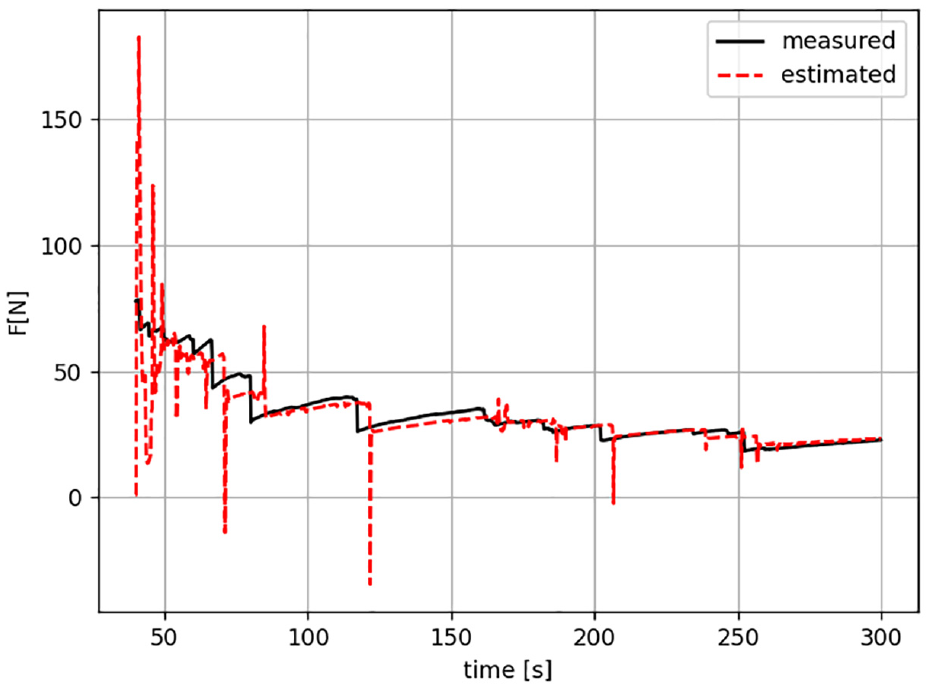
The crack length estimation is performed in this section by considering 4 strain measurements on the upper arm (Table 4). Further 4 strain “dummy” strain measurements have been considered for the lower arm given the symmetry of the system. The pROM was computed as described in Sec. Reduction basis and the size of the reduced model is set to $r = 67$ . Contrarily to the numerical case study presented above, the local bases are computed by sub-sampling the interface every 3 springs. This means that the process zone is intrinsically $n_{pz} = 3$ with a constant parameter distribution law, that is, $p_{pz} = [111]^{T} p^{l}$ . This choice allows to reduce the size of the pROM and thus its computational cost. For future validation, the knowledge of the process zone is needed and for example, Digital Image Correlation (DIC) techniques can be employed to this end. Figure 24(a), (b), and (e) show respectively the estimation of measured data, strain field and crack length obtained by assuming known loads being applied to the FE model. Figure 24(c), (d), and (e) show measured data, strain field and crack length when the loads are unknown and estimated (Figure 25). As before, constant loads with very low amplitude of $1 N$ are applied during the estimation in order to guarantee the system observability. The estimated force shows some peaks corresponding to the jumps observed on the measured strain data, which are a typical behavior of woven fabric materials.⁴¹ At those points, some additional modelling errors, for example, boundary conditions, occur and the linear FE model cannot match the measurements. As shown in the numerical validation section, the modelling errors are therefore compensated by the KF in the force estimation since higher covariance values have been assumed for the augmented states corresponding with the unknown loads as compared with the parameters, that is, $Q_{u} > > Q_{p}$ . In conclusion, the joint input/parameter estimation accurately predict the critical load and provide full-field reconstruction even when employing a less-correlated, that is, less accurate, linear model. The joint estimation is more advantageous with respect to parameter-only estimation, that is, the scenario with known loads, since the modelling errors are then compensated by both the estimated loads and parameters and not fully and only by parameter degradation, and both quantities (loads and parameters) show good levels of estimation accuracy.

Figure 24.

AEKF recursive estimation results on experimental DCB. (a) Known loads: measured (red) versus estimated (black) strain (upper lamina), (b) known loads: estimated (unmeasured) strain, (c) unknown loads: measured (red) versus estimated (black) strain (upper lamina), (d) unknown loads: estimated (unmeasured) strain, and (e) estimated crack length.

Figure 25.

Estimation of reaction force for the experimental DCB.

Conclusions

This work addresses the delamination growth monitoring in composite materials by employing the extended augmented Kalman filter. The proposed methodology is validated on simulated and experimental data for a composite DCB specimen. A simplified linear FEM is employed in the estimator. This provides a great advantage from modelling point of view and computational costs. However, the usage of shell elements connected with node-to-node springs does not constrain rotations at the crack tip and this leads to an under-prediction of the reaction force when the damage initiates and propagates. The estimation error observed on the force is $< 6 %$ for both analyzed numerical models. The simplified model reaches a good level of accuracy also when using experimental data. A recursive parameter estimation scheme for interface stiffness degradation is proposed to reduce the number of sensors needed for the system observability. The stiffness parameter distribution embedded in the estimator allows to consider the effect of the process zone developing during the delamination propagation. The study of sensors networks shows that a single position-level measurement is enough to monitor the crack propagation when the loads are known. During operation, the critical loads causing the damage are however typically unknown and thus the joint input/parameter estimation is also addressed in this contribution, showing that the estimation accuracy increases with the number of collocated measurements. The implementation of this methodology on a real test case needs thus to sensorize the critical area of interest to monitor the damage growth and estimate the critical loads. Future investigation aims to evaluate a more accurate and advanced study on the stiffness distribution within the process zone and to explore a possible improvement of the estimation by employing embedded sensors, such as for example, FBGs. Implementation on a more complex test-case will be also addressed.

Footnotes

Acknowledgements

The authors acknowledge R&D team of Leonardo Aerostructure Division for its support in the experimental validation.

Declaration of conflicting interests

The author(s) declared no potential conflicts of interest with respect to the research, authorship, and/or publication of this article.

Funding

The author(s) received no financial support for the research, authorship, and/or publication of this article.

ORCID iD

Roberta Cumbo

References

Ostachowicz

Soman

Malinowski

Optimization of sensor placement for structural health monitoring: a review. Struct Health Monit 2019; 18(3): 963–988.

Sun

Büyüköztürk

Optimal sensor placement in structural health monitoring using discrete optimization. Smart Mater Struct 2015; 24(12): 125034.

Flynn

Todd

MD.

A Bayesian approach to optimal sensor placement for structural health monitoring with application to active sensing. Mech Syst Signal Proc 2010; 24(4): 891–903.

Zou

Tong

LPSG

Steven

GP.

Vibration-based model-dependent damage (delamination) identification and health monitoring for composite structures—a review. J Sound Vibrat 2000; 230(2): 357–378.

Moorthy

Marappan

Experimental study on delamination identification in tapered laminated composite plates using damage detection models. Compos Struct 2023; 323: 117494.

Kralovec

Schagerl

Review of structural health monitoring methods regarding a multi-sensor approach for damage assessment of metal and composite structures. Sensors 2020; 20(3): 826.

Tuloup

Harizi

Aboura , et al. On the use of in-situ piezoelectric sensors for the manufacturing and structural health monitoring of polymer-matrix composites: a literature review. Compos Struct 2019; 215: 127–149.

Dou

, et al. Piezoelectric materials and sensors for structural health monitoring: fundamental aspects, current status, and future perspectives. Sensors 2023; 23(1): 543.

Aabid

Parveez

Raheman

, et al. A review of piezoelectric material-based structural control and health monitoring techniques for engineering structures: challenges and opportunities. Actuators 2021; 10(5): 101.

10.

Takeda

Minakuchi

Okabe

, et al. Delamination monitoring of laminated composites subjected to low-velocity impact using small-diameter FBG sensors. Compos Part A Appl Sci Manuf 2005; 36(7): 903–908.

11.

Panopoulou

Loutas

Roulias

, et al. Dynamic fiber Bragg gratings based health monitoring system of composite aerospace structures. Acta Astron 2011; 69(7–8): 445–457.

12.

Kuang

KSC

Cantwell

. Use of conventional optical fibers and fiber Bragg gratings for damage detection in advanced composite structures: a review. Appl Mech Rev 2003; 56(5): 493–513.

13.

Gholizadeh

A review of non-destructive testing methods of composite materials. Proc Struct Integr 2016; 1: 50–57.

14.

Cristiani

Falcetelli

Yue

, et al. Strain-based delamination prediction in fatigue loaded CFRP coupon specimens by deep learning and static loading data. Compos Part B Eng 2022; 241: 110020.

15.

Tidriri

Chatti

Verron

, et al. Bridging data-driven and model-based approaches for process fault diagnosis and health monitoring: a review of researches and future challenges. Ann Rev Control 2016; 42: 63–81.

16.

Wang

Ramakrishnan

, et al. A comparison of machine learning algorithms for assessment of delamination in fiber-reinforced polymer composite beams. Struct Health Monit 2021; 20(4): 1997–2012.

17.

Ramakrishnan

Wang

, et al. A combined global-local approach for delamination assessment of composites using vibrational frequencies and FBGs. Mech Syst Signal Proc 2022; 167: 108577.

18.

Cumbo

Tamarozzi

Janssens

, et al. Kalman-based load identification and full-field estimation analysis on industrial test case. Mech Syst Signal Proc 2019; 117: 771–785.

19.

Risaliti

Tamarozzi

Vermaut

, et al. Multibody model based estimation of multiple loads and strain field on a vehicle suspension system. Mech Syst Signal Process 2019; 123: 1–25.

20.

Capalbo

De Gregoriis

Tamarozzi

, et al. Parameter, input and state estimation for linear structural dynamics using parametric model order reduction and augmented Kalman filtering. Mech Syst Signal Proc 2023; 185: 109799.

21.

Naets

Croes

Desmet

An online coupled state/input/parameter estimation approach for structural dynamics. Comput Methods Appl Mech Eng 2015; 283: 1167–1188.

22.

Cumbo

Mazzanti

Tamarozzi

, et al. Advanced optimal sensor placement for Kalman-based multiple-input estimation. Mech Syst Signal Proc 2021; 160: 107830.

23.

Hong

Epureanu

Castanier

MP.

Next-generation parametric reduced-order models. Mech Syst Signal Process 2013; 37(1–2): 403–421.

24.

Amsallem

Farhat

An online method for interpolating linear parametric reduced-order models. SIAM J Sci Comput 2011; 33(5): 2169–2198.

25.

Zahr

Farhat

Progressive construction of a parametric reduced-order model for PDE-constrained optimization. Int J Numer Methods Eng 2011; 102(5): 1111–1135.

26.

Benner

Gugercin

Willcox

A survey of projection-based model reduction methods for parametric dynamical systems. SIAM Rev 2015; 57(4): 483–531.

27.

CSN EN 6033. Carbon fibre reinforced plastics—test method—determination of interlaminar fracture toughness energy—mode I—GIC. Aerospace Series, 2015.

28.

Park

Paulino

GH.

Cohesive zone models: a critical review of traction-separation relationships across fracture surfaces. Appl Mech Rev 2011; 64(6): 060802.

29.

Dimitri

Cornetti

Mantič

, et al. Mode-I debonding of a double cantilever beam: a comparison between cohesive crack modeling and finite fracture mechanics. Int J Solids Struct 2017; 124: 57–72.

30.

Zienkiewicz

Taylor

RL.

The finite element method: solid mechanics (Vol. 2). Oxford, UK: Butterworth-Heinemann, 2000.

31.

Simon

Optimal state estimation: Kalman, H infinity, and nonlinear approaches. Hoboken, NJ: John Wiley and Sons, 2006.

32.

Azam

Chatzi

Papadimitriou

A dual Kalman filter approach for state estimation via output-only acceleration measurements. Mech Syst Signal Proc 2015; 60: 866–886.

33.

Lourens

Reynders

De Roeck

, et al. An augmented Kalman filter for force identification in structural dynamics. Mech Syst Signal Proc 2012; 27: 446–460.

34.

Tamarozzi

Risaliti

Rottiers

, et al. Noise, ill-conditioning and sensor placement analysis for force estimation through virtual sensing. In: International conference on noise and vibration engineering (ISMA2016), pp. 1741–1756. Belgium: Katholieke Univ Leuven, Department Werktuigkunde, 2016.

35.

McElroy

. An enriched shell element for delamination simulation in composite laminates. In: American Society for Composites technical conference (No. NF1676L–20621), East Lansing, MI, USA, 28–30 September 2015.

36.

Craig

Jr.

A review of time-domain and frequency-domain component mode synthesis method. Int J Analyt Exp Modal Anal 1987; 2(2): 59–72.

37.

Skec

Alfano

Jelenic

Complete analytical solutions for double cantilever beam specimens with bi-linear quasi-brittle and brittle interfaces. Int J Fract 2019; 215: 1–37.

38.

Berry

JP.

Determination of fracture surface energies by the cleavage technique. J Appl Phys 1963; 34(1): 62–68.

39.

Williams

JG.

The fracture mechanics of delamination tests. J Strain Anal Eng Design 1989; 24(4): 207–214.

40.

ASTM D5528/D5528M-21. Standard test method for mode I interlaminar fracture toughness of unidirectional fiber-reinforced polymer matrix composites. West Conshohocken, PA: ASTM International, 2022.

41.

Fanteria

Lazzeri

Panettieri

, et al. Experimental characterization of the interlaminar fracture toughness of a woven and a unidirectional carbon/epoxy composite. Compos Sci Tech 2017; 142: 20–29.