
Abstract
This article introduces a novel methodology for detecting and classifying anomalies in multiple bridges within a geographical region using satellite-based interferometric synthetic aperture radar displacements and environmental measures. The approach uses subspace alignment to harmonize bridge features, enabling the detection of anomalies based on deviations in one bridge compared to the rest of the population. Simulated and real case studies involving steel railway bridges spanning the Po River in Italy demonstrate the effectiveness of the proposed approach, showcasing its potential for large-scale applications. Moreover, the study explores the transferability of knowledge from simulated data to real-world monitoring scenarios, yielding promising results in classifying real instances using synthetic labels. The proposed approach presents practical benefits for bridge monitoring agencies by providing a cost-effective method for enhancing the resilience and safety of transportation infrastructure.
Keywords
Introduction
Recent progress in managing transportation infrastructure increasingly relies on data-driven approaches, using sophisticated integration techniques that lean toward the emerging concept of “digital twin.” 1 Initially proposed for individual structures, digital twins have recently expanded to encompass entire regions. 2 They aim to model the complex relationships between multiple structures and infrastructures, their inputs, and the consequences of failure and performance reductions of critical elements. This modeling proves invaluable for assessing the resilience of transportation networks, a topic gaining significant traction due to well-documented recent climate-related emergencies. 3
Among the crucial components of transportation networks, bridges hold paramount importance. Monitoring bridge conditions typically requires extensive sensing. 4 However, the abundance of sensors entails considerable deployment, maintenance, and management costs. To tackle these challenges, ongoing research in bridge structural health monitoring (SHM) is shifting toward cost-effective data acquisition technologies. These include remote satellite-based sensing, which eliminates the need for installing on-site sensors.
Notably, synthetic aperture radar interferometry (InSAR), initially employed for monitoring land movements, has recently achieved remarkable sensitivity owing to evolving technologies. 5 This approach leverages synthetic aperture radar (SAR) devices aboard orbiting satellites to deliver high-resolution, weather-independent imagery of the Earth’s surface. Various natural and man-made structures, such as rocks, building roofs, and road surfaces, strongly reflect the electromagnetic signals emitted by radars, which capture the back-scattered signals, thus generating SAR images. Displacement time series for specific reflective elements, known as persistent scatterers (PSs), can then be obtained by applying specific algorithms on multiple images, achieving millimetric precision along the line of sight connecting the SAR sensor to these points. 6
Due to its high sensitivity, this strategy has recently been exploited for static monitoring of several civil structures, such as bridges. Significant advantages include the widespread availability of data—virtually, from the entire globe—and access to historical records—now spanning over a decade. Consequently, it enables investigations into the causes behind structural issues in bridges that were never equipped with dedicated sensing systems.7–13 Since the displacement measurements obtained via InSAR are static, the types of damage that can be identified remotely include scouring/erosion effects,10,11,14 differential displacements due to local settlements,12,13,15 land subsidence/uplift,7,16 and deck deformation.8,9 Literature contributions in this field also analyze bridge deformation induced by seasonal thermal effects, which exhibit a characteristic fluctuating pattern with a yearly cycle,17–24 and the correlation between displacements and water levels.25–28 In addition, InSAR-based monitoring has become particularly appealing for monitoring infrastructure networks in wide geographical regions. 29
In the current literature, scholars have demonstrated how InSAR data can complement or precede SHM strategies based on on-site systems, noting that both methods generally align in measuring displacement trends, though satellite measurements may sometimes be unavailable for specific structures or less accurate than field measurements.30,31 Additionally, methods traditionally used for on-site monitoring have been applied to InSAR data to detect anomalous behavior of different types of structures. For instance, Bonaldo et al. 32 analyzed the residuals of autoregressive models trained on 3 years of multitemporal (MT)-InSAR displacement data obtained from COSMO-SkyMed images to detect anomalies for Palazzo Primoli in Rome (Italy). Selvakumaran et al. 10 processed several TerraSAR-X images over the Tadcaster Bridge (England), highlighting the reliability of MT-InSAR methods to identify anomalous displacements in a region of the bridge where partial collapse occurred due to scour. Similarly, Sousa and Bastos 11 used MT-InSAR data to study the displacement time history that preceded the collapse of the Hintze Ribeiro bridge across the Douro River. The authors confirmed the possibility of implementing an early warning system based on the definition of displacement alarm thresholds based on static remote measurements. Also, Cusson et al. 33 employed satellite monitoring as an early warning mechanism for unexpected displacements. De DePrekel et al. 34 investigated the gradual displacement of some bridges in California, attributing the movements to subsidence phenomena resulting from continuous water extraction from nearby aquifers. Milillo et al. 8 discussed relative deformations of the Morandi Bridge (Italy) recorded before its collapse in 2018.
An effort to reconstruct the two-dimensional displacement field was undertaken by Farneti et al., 12 gathering displacement data from both ascending and descending geometries for the Albiano-Magra viaduct, which collapsed in 2020. The authors also analyzed the displacements of surrounding areas, which provided key information for determining the possible causes of the collapse. In a following study, Farneti et al. 13 combined the information obtained through InSAR measurements with numerical modeling to predict the service life of the Albiano-Magra viaduct. Lately, several scholars have employed numerical models to help interpret or predict displacement trends of monitored structures and to calibrate structural properties. Vázquez-Ontiveros et al. 35 assessed the risk of dam failure by monitoring radial displacements at various reservoir levels, using refined finite element (FE) models for interpretation. Similarly, Guzman-Acevedo et al. 36 proposed a risk assessment methodology to estimate a safety index of bridges using InSAR data and a calibrated FE model based on stress limits provided by the American Association of State Highway and Transportation Officials. Zhou et al. 37 obtained an advanced temperature field model within the elements of a steel arch bridge using meteorological data available online, including temperature, wind speed, and precipitation. The authors used both environmental and InSAR data to refine the thermal dilation phase in their bridge model.
Typically, prior knowledge of structures is required to develop the models used in these studies for reliably interpreting InSAR measurement results. 30 Additionally, most of the referenced articles focus on individual bridges, comparing their current state with their past behavior to identify any variations potentially linked to damage. This approach is commonly employed in civil SHM. The inherent dissimilarities among different bridges prevent the direct comparison between their behaviors to detect anomalies. Conversely, direct comparison is frequently used in fault detection within other domains, such as mechanical engineering, for identical machinery components.
Recently, population-based SHM (PBSHM) has emerged as a strategy to transfer knowledge across various bridges deemed sufficiently “similar.” 38 This approach aims to infer damage classification information by leveraging data from bridges with documented similar behaviors. 39 In civil engineering, this is mainly achieved through domain adaptation (DA) algorithms. DA, a specific type of transfer learning method, addresses discrepancies between “source” and “target” features (i.e., parameters that describe the structural behavior) with distinct marginal and class-conditional distributions, aiming to minimize their disparity. 40 Consequently, aligned features can train damage classifiers applicable to both the source and target structures.
To date, PBSHM has predominantly focused on dynamic features. Gardner et al. 41 explored DA concepts for vibration-based SHM in multistory buildings. In the realm of bridge SHM, Poole et al. 42 used statistic alignment, one of the simplest DA techniques, to align natural frequencies from different bridges, namely, the Z24 and KW51 bridges, showcasing its efficacy in recognizing environmental variations. Similarly, Giglioni et al. 39 demonstrated improved damage detection by applying different DA methods between the Z24 and S101 bridges. Omori Yano et al. 43 employed various transfer learning strategies across bridges, including transfer component analysis (TCA), joint DA, and maximum independence DA. Additionally, Figueiredo et al. 44 proposed employing TCA to harmonize classifiers between real bridge data and simplified numerical models.
The widespread availability of satellite data facilitates the acquisition of datasets encompassing a vast array of similar bridges in large regions. Additionally, access to historical data renders alignment strategies and DA approaches accessible. Nevertheless, static measures have never been explored for damage-related knowledge transfer. Therefore, novel features must be devised to be damage-sensitive (considering the types of damage observable through InSAR data) and maintain consistency across bridges (irrespective of the number of PSs identified by the InSAR methods) when transfer learning algorithms are applied.
This study introduces an innovative approach to anomaly detection and characterization that reduces reliance on past experiences of monitored structures. This aspect is critical in light of climate change and the rising frequency of severe weather events, aiming to mitigate the risk of false alarms stemming from environmental factors previously unencountered by the monitored bridges. 45
Specifically, the study proposes a methodology for “regional-scale” SHM, which addresses a typical challenge faced by management administrations that cannot afford to instrument all bridges in their area of interest, but require data for territorial analyses, such as evaluation of the resilience of the transportation network. The proposed methodology considers a population of similar bridges within a confined geographical area. The underlying assumption is that these bridges share similar structural properties (i.e., geometry and boundary conditions) and environmental factors influencing their static response, such as temperature variations and the fact that they traverse the same river.
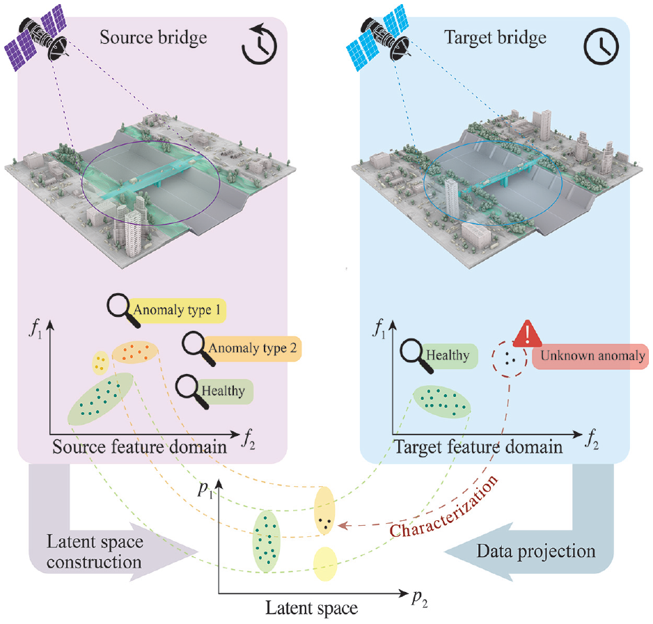
The proposed strategy is finalized to detect anomalous bridge displacements, which may potentially lead to failure mechanisms. It operates on the premise that bridges with similar designs and environmental drivers should exhibit comparable structural responses over time. However, direct comparisons in physical space are hindered by the unique characteristics of each bridge. To address this challenge, this study proposes using subspace alignment (SA) to render bridge static features comparable within a latent domain shared by all bridges. An anomaly index is then defined in this domain based on instantaneous differences between bridge behaviors. Next, a methodology for inferring information about the type of anomaly is introduced, using synthetic bridge models for simulation-to-real knowledge transfer. The feasibility of a meaningful knowledge transfer relies on the similarity between the developed models and real bridges, which share common features, including structural schemes and dimensions, riverbed topography, and environmental conditions.
This approach introduces the following key innovations: (1) it applies PBSHM to InSAR data for the first time, defining a tailored set of static damage-sensitive features; (2) it shifts monitoring from individual time-based comparisons to relative instantaneous comparisons, reducing the dependence on historical data; and (3) it relies solely on publicly available data (InSAR and environmental measures) accessible online, potentially applicable to bridges worldwide.
The next section outlines the proposed methodology for regional-scale bridge monitoring and introduces the selected case study and the data employed in this research. The approach is then demonstrated using simplified bridge models to simulate various types of anomalies, both physical and computational. Finally, the proposed method is applied to a real case study involving a population of seven steel railway bridges spanning the Po River in Italy. Final remarks are drawn in the Conclusions.
Regional-scale bridge monitoring
In traditional SHM procedures, when real-world environmental conditions differ from those used to train anomaly detection models, false positives can occur due to unexpected data trends.46,47 This study introduces a method that compares the responses of similar bridges to shared environmental inputs. Given the low likelihood of all bridges experiencing structural anomalies simultaneously, if multiple bridges exhibit behavior that deviates from their historical patterns, it is more probable that the anomaly is due to an unusual environmental driver. Conversely, actual anomalies are identified if only a small subset of bridges reacts differently from the rest under the same environmental inputs. This approach helps minimize false alarms. Since environmental inputs are not identical for all monitored structures, and their responses may vary depending on the individual bridge characteristics, a DA process is applied to preprocess the bridge features.
The proposed methodology consists of the following steps:
Similarity assessment: a population of bridges is formed according to similarity criteria regarding their structural behavior.
Initialization and feature extraction: all available datasets (in this study, displacement and environmental data) are encoded into standardized structural features and projected onto a common latent domain using DA.
Anomaly detection: abnormal behaviors within one or more bridges are identified using a damage indicator that considers the disparities between the behavior of bridge features in the latent domain.
Anomaly characterization: the features of anomalous bridges are classified using a machine learning-based model trained on “source” bridge(s) with available anomaly labels.
This method assumes that a set of anomalous behaviors has already been recognized and labeled for the source bridges. This recognition may involve interpreting data from additional sensors (such as dynamic sensing systems, strain gauges, or riverbed-level sensors) or conducting visual inspections to validate anomalous conditions that may have occurred in the past. The gathered information is then transferred from the source domain to the target domain, which includes bridges with limited knowledge regarding their condition. Noteworthy, if labels are not initially available for any bridges in the population, they can be assigned during the monitoring process as soon as a new anomaly is detected and validated through visual inspections or professional interpretations involving a human-in-the-loop process. 48 This allows for the continual enrichment of the label database throughout the monitoring lifespan, gathering labels for various phenomena that may impact any bridge within the population.
Similarity assessment
Recent research has delved into the prerequisites necessary for structures within a population to achieve “positive transfer,” whereby knowledge transfer effectively enhances anomaly classification outcomes. In this regard, scholars have proposed a method of conceptualizing structures using irreducible element models, which are simplified representations of structural components, and encoding them into attributed graphs (AGs). 38 AGs consist of compact representations of the connections between elements alongside their pertinent information, such as material, size, and shape. This process becomes crucial when the features used in anomaly identification are closely linked to these characteristics and are sensitive to their variations. For instance, in studies that use natural frequencies for vibration-based PBSHM, it is fundamental to ensure similarity in connections, material properties, and geometric characteristics, all of which influence the mass and stiffness of the systems.
This study uses structural features derived from static displacement measures to identify structural anomalies (i.e., excessive displacements) potentially related to incipient failure mechanisms in statically determinate structures. As a result, material properties and cross-section geometry become less significant. Conversely, ensuring consistency in the structural configuration (i.e., the connections between decks and piers) in all bridges within the population is essential.
Thus, the similarity assessment needed by the proposed approach is less stringent than the one commonly employed for vibration-based problems, prompting avenues for further exploration. Future studies will pursue specific investigations in this direction.
The case study investigated in this article comprises seven railway steel bridges (B1–B7) spanning the Po River in Italy, depicted in Figure 1. All these bridges consist of simply supported truss elements supported by piles, some of which are located within the river. Additionally, the bridge spans are of similar lengths, ranging approximately between 65 and 85 m. Consequently, the bridges in this case study have comparable structural configurations and face similar environmental conditions, as detailed in the following sections.
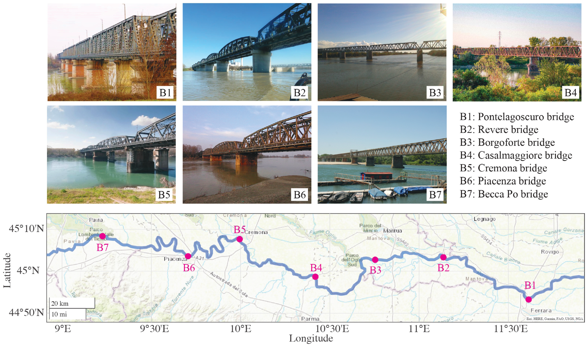
Selected case study on the Po River, Italy.
Initialization and feature extraction
The displacement data used in this study consist of InSAR Sentinel-1 data, postprocessed to derive purely vertical displacement components at a regular grid of control points. These data were acquired by fusing PSs identified from ascending and descending orbit satellites and interpolating measurements to a 100 m grid. This study did not involve the extraction of displacement time histories from SAR images. Instead, the displacement data were sourced from the European Ground Motion Service (EGMS) as part of the Copernicus project. 49 Comprehensive details regarding the algorithms and parameters used to generate this data are available in the EGMS technical documentation. 50 The employed data span two time intervals: (I1) January 5, 2016 to December 22, 2021, and (I2) January 6, 2018 to December 17, 2022. Displacement time histories for these intervals were obtained individually from different InSAR image sets, causing noncoincidence in the data during the overlapping period. The original sampling period of both displacement datasets is every 6 days. The displacement data refer to the control points depicted in Figure 2. Specifically, the number of control points extracted for bridges B1–B7 are 7, 11, 4, 9, 14, 12, and 11, respectively. Bridge areas that delimit the employed control points were defined manually.
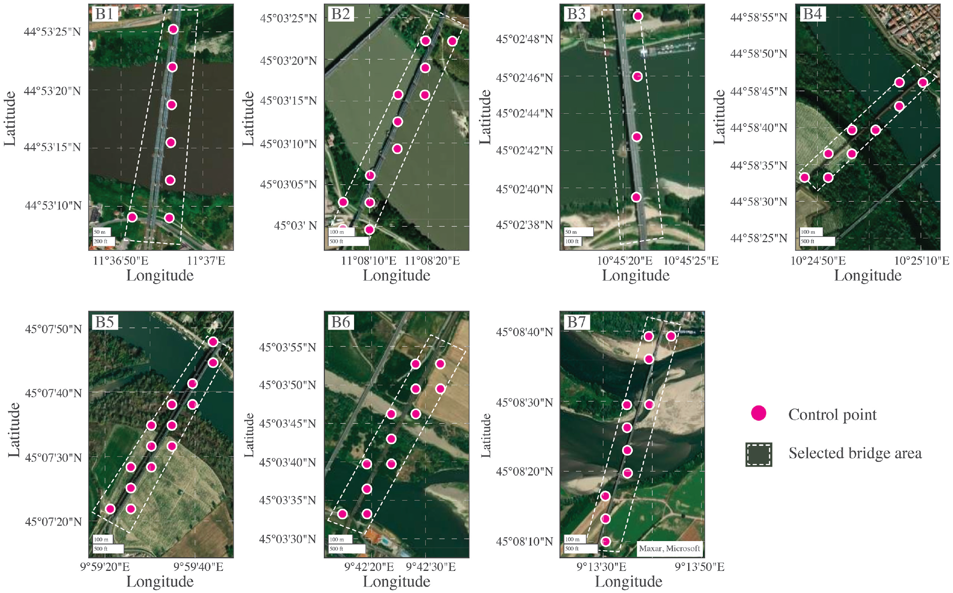
Satellite views of the selected bridges and control points for vertical displacements.
The displacements at control points represent an average quantity estimated within the respective grid element with millimeter-level accuracy. 50 However, it is crucial to note that vegetation and water do not generate PSs. Consequently, the control points available are likely only representative of the bridge movements.
Environmental data analyzed in this article encompass air temperature, water level, and water discharge measured close to the selected bridges. Specifically, air temperature 2 m above the land surface was sourced from ERA5-Land Copernicus datasets. 51 These datasets are available at a 10 km grid and hourly time discretization. Water level information was obtained from hydrographic monitoring stations managed by the Interregional Agency for the Po River (AIPo), accessible online via the agency website. 52 Sampling periods for water level vary between 5 and 10 min depending on the specific monitoring station. Water discharge data near selected bridges were obtained from the Dext3r service, a web system provided by the Regional Agency for Prevention, Environment, and Energy of Emilia-Romagna (ARPAE). 53 Environmental data were acquired for the entire time interval enclosing I1 and I2, as depicted in Figure 3. Noteworthy, air temperatures and the water discharge observed for all the considered bridges exhibit remarkable similarities.
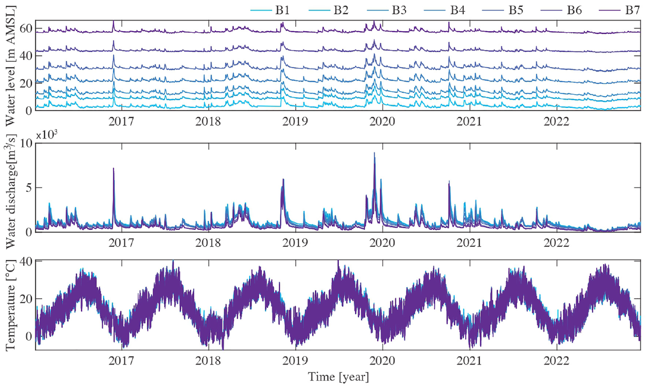
Environmental measurements taken for the selected bridges in the analyzed time interval.
The first step of data initialization involves resampling the displacement and environmental data onto a fixed temporal grid. This is achieved by applying linear interpolation to displacement data to obtain a daily sampling period. On the other hand, environmental data were first processed through a moving average process with a 1-day window and then subsampled to have the same sampling period as displacement data.
In this process, two distinct datasets were created: the first spans from January 5, 2016 to November 13, 2019 (using InSAR data from I1), and the second spans from November 14, 2019, to December 17, 2022 (using InSAR data from I2). In the following, these datasets are termed the “reference” and “monitoring” time intervals, respectively.
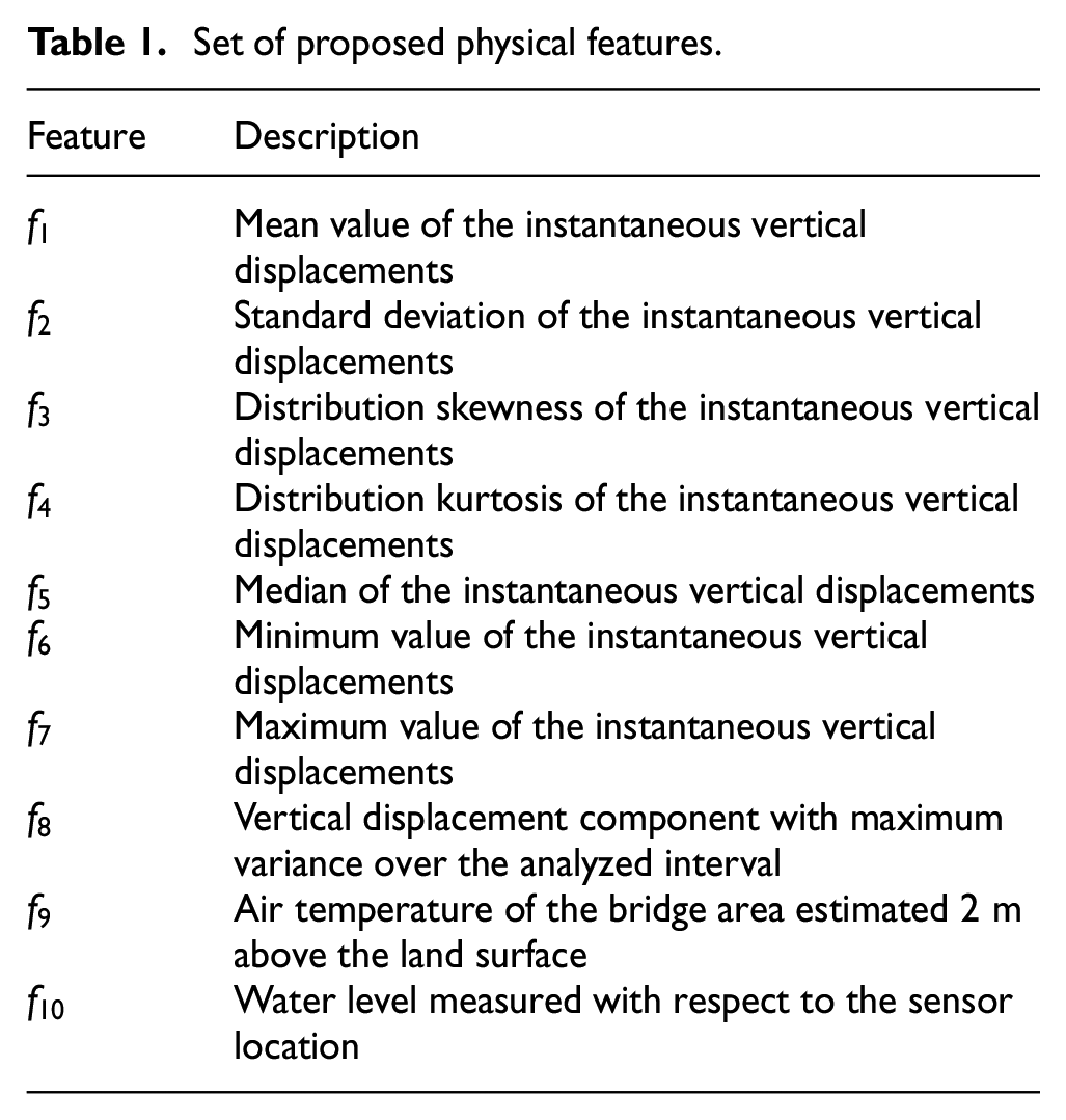
Upon resampling, a set of features is extracted from the data. Due to limitations inherent to InSAR technology and displacement extraction algorithms, the displacement time histories are not tied to specific locations on the selected bridges but should be understood as average displacements (with associated uncertainties) within each square area of the 100 m grid. This introduces two main challenges for feature extraction: (1) different bridges typically have varying numbers of control points, and (2) it is impossible, with the data type used in this study, to reference displacements to a specific part of the structure. Nonetheless, these displacements can effectively capture the overall behavior of the structure on a scale roughly equivalent to its span size. These constraints led to defining features that condense the information into global indicators, such as average displacements and the distribution of displacements at control points relative to the average (i.e., statistical moments). Specifically, this study proposes the features listed in Table 1. In defining them, four possible anomalies were considered: scouring (Sc) processes, which typically result in global stiffness reductions in pier foundations due to vortexes that lower the riverbed depending on water speed and bridge geometry54,55; differential settlements (Se), involving anelastic displacement of selected piers downwards; uplifts (Up), similar to settlements but involving upward displacements; and outliers (Ou), a typical anomaly associated with InSAR data, for instance, due to changes of a PS from one physical element to another within the spatial grid.
Set of proposed physical features.
The features outlined in Table 1 pose challenges for direct comparison across different bridges due to inherent differences between the individuals of the population, that is, the features (
Scheme of the data projection process and anomaly characterization using subspace alignment.
An example of feature distributions before (
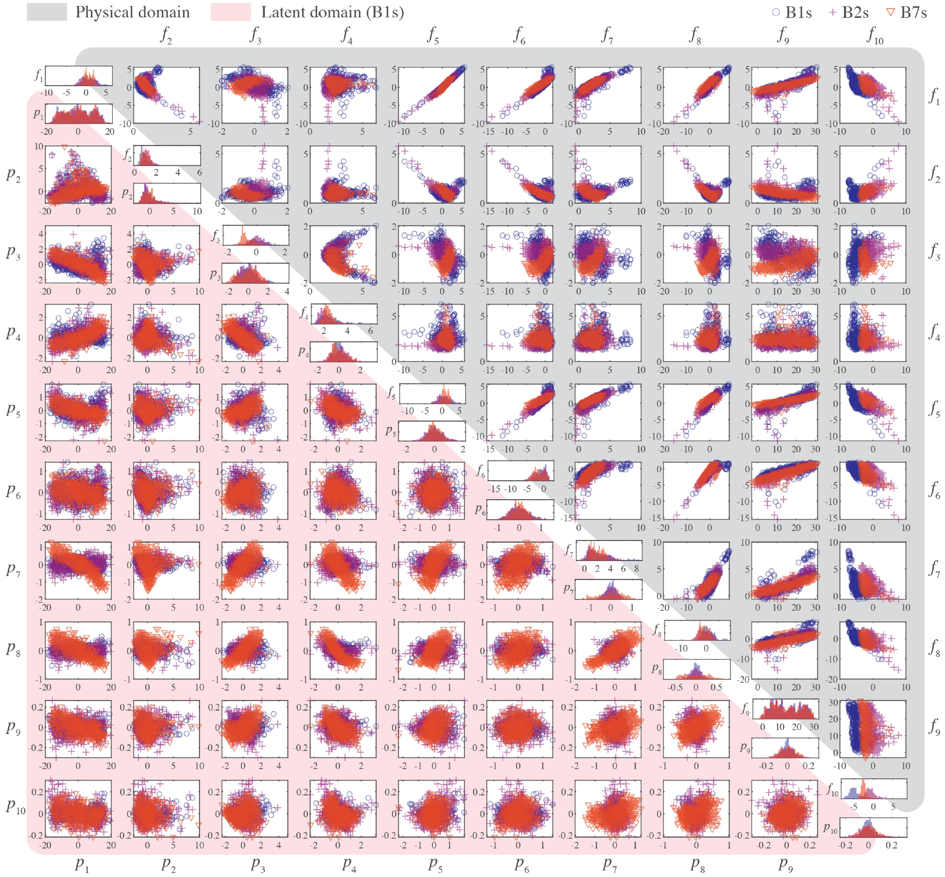
2D visualizations of the synthetic features of three bridges, namely B1s, B2s, and B7s, before (gray region) and after (red region) projection onto the latent domain (with source B1s) using subspace alignment. The plots on the diagonal represent the probability density distributions of the features.
While extensive details on SA implementation can be found in relevant literature,
56
a brief theoretical background is reported herein, together with a scheme that represents its application in the context of this study (see Figure 6). Let
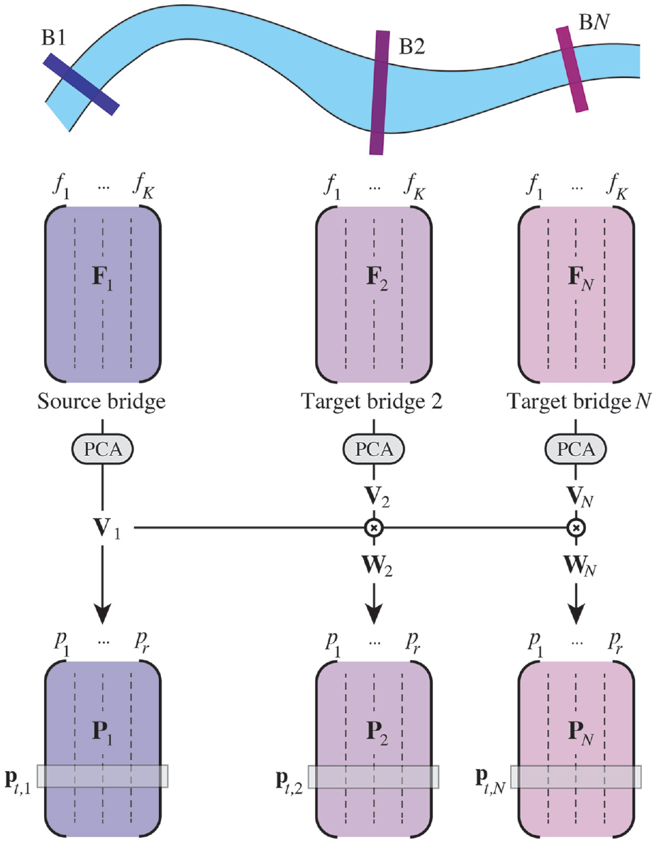
Scheme of the data harmonization process based on subspace alignment.
First, a mean centering process was applied to every column of
The target data can thus be projected onto a source-aligned coordinate system according to the projection matrix 56 :

This matrix transforms the target subspace coordinates into the source subspace coordinates by aligning the target basis vectors with the source ones. Therefore, the source and target data projected onto the source subspace (i.e., the latent space) can be obtained as, respectively:


In this study,
The main computational complexity of SA lies in calculating the projection matrices of feature time histories through PCA. This operation has a complexity of
It is worth noting that if the projection process is executed during the same reference time interval for all bridges, assumed unaffected by anomalies, the same projection matrices can be used for subsequent monitoring intervals. Furthermore, due to the similarities in environmental drivers, projected features of different bridges should move together in the latent space over time.
Anomaly detection
Under regular conditions, the responses of bridges should exhibit similar trajectories within the source subdomain. However, if anomalies occur, denoting changes in the relationship between bridge features, the data from affected bridges would diverge from the average trajectory. This divergence occurs because the original projection matrix cannot accurately represent the new relationship between features. Moreover, if two or more bridges experience the same anomaly, their features should converge to the same region within the source subdomain. Figure 7 schematizes the proposed anomaly identification process, and in particular, Figure 7(a) illustrates this situation in a 2D representation of the latent space.
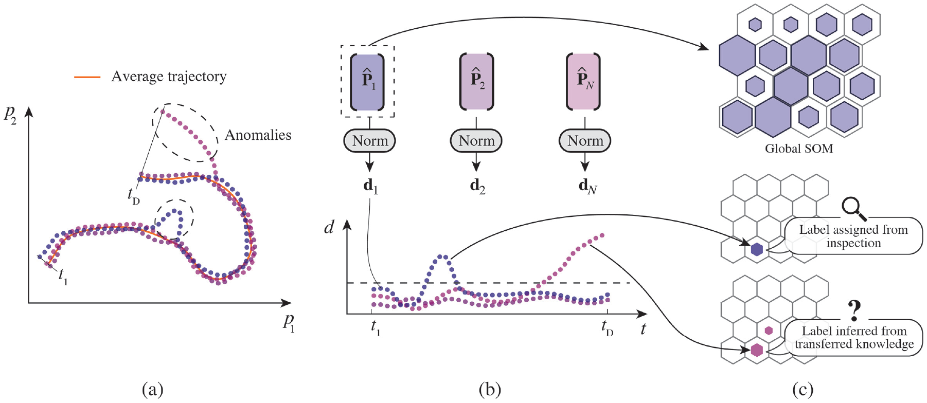
Proposed monitoring workflow: (a) calculation of the average trajectory, (b) anomaly detection using the relative distance metric, and (c) anomaly classification using knowledge transfer.
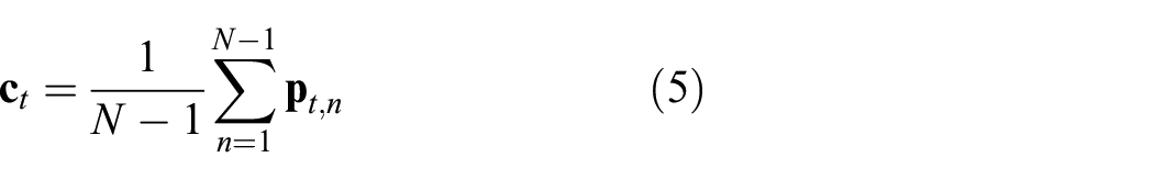
Following this rationale, for each bridge, an anomaly index is defined at time

with
Various methods exist for calculating the centroid. In this step, special attention must be given to eliminating anomalous data points, which could affect the detection results. One approach could entail training an autoregressive model with exogenous input to estimate the centroid position at time point
where
A threshold for anomaly detection can then be established either by leveraging historical data or employing outlier detection methods based on the instantaneous distribution of distances from the centroid. In the former approach, conventional methods can be used to determine an acceptable probability of false alarms (or errors in damage detection) using data from a reference period. Specific techniques, such as the receiver operating characteristic curve, can aid in determining optimal thresholds. 59 Alternatively, reliance on historical data can be entirely eliminated from the methodology in the latter approach. However, a larger population might be required to establish a statistically significant threshold. This study adopts the former approach, acknowledging that dependence on historical data can be removed by increasing the number of bridges within the considered population.
Anomaly characterization
The recentered datasets (denoted as
This study proposes training a self-organizing map (SOM) 60 with the available data. SOMs are unsupervised learning models commonly used for data visualization, capable of generating low-dimensional representations of high-dimensional data distributions. By creating a SOM with the available dataset, a low-dimensional map with a selected number of nodes and links is formed, where nodes represent centroids of clusters identified in the data. After conducting the unsupervised training process, labeled data can be fed to the SOM to assign relevant labels to the cluster(s) they belong to (see Figure 7(c)).
Subsequently, unlabeled anomalies can be processed through the SOM. If they are assigned to a cluster with an available label, this label can be used to infer the type of anomaly. On the other hand, if anomalous data are assigned to unlabeled clusters, new labels can be assigned afterward through a human-in-the-loop process involving visual inspections to ascertain the causes behind anomalies on affected bridges.
In contrast to simpler clustering algorithms like k-means, SOMs preserve the topological structure of data, giving physical meaning to close clusters exhibiting similar features. 61 Once trained, the SOM can be deployed for future classification, focusing solely on newly identified anomalies.
Simulated benchmark
An initial demonstration is conducted using numerical models of the bridge population to assess the procedure using known anomalies. Specifically, seven bridges were modeled in 2D, considering the plane orthogonal to the water flow. Here, simulated bridges are labeled as “B#s,” while real bridges are denoted as “B#.” Despite their simplicity, the models are designed to effectively capture the primary factors influencing the measured structural output, that is, static displacements. The geometric parameters in the developed models closely resemble real-world conditions, while the employed environmental drivers consist of the real measurements described in the section Data description.
Model description
The geometries of the bridges were generated based on topographic measurements of the river sections obtained from the AIPo website. 62 While the number and positions of the piles do not precisely replicate the real configurations, they were adjusted to have spans of approximately 72 m, resembling real-world scenarios. 63 A schematic representation of the modeled bridges is provided in Figure 8.
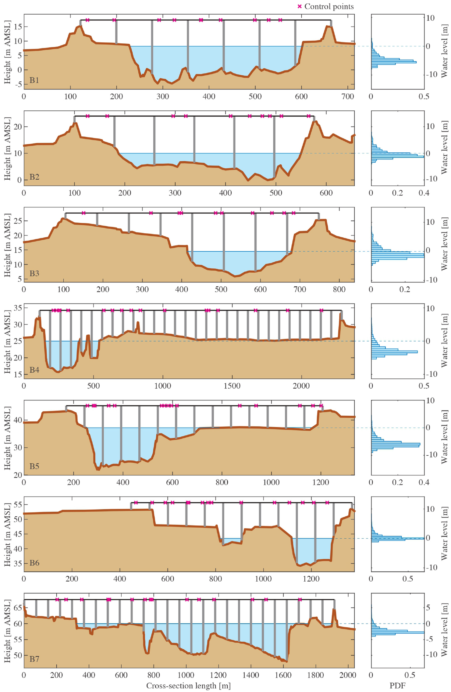
Cross-section profile of the selected bridges and probability density distribution of the water level (with respect to the sensor location) in the studied time interval.
To simulate realistic datasets, actual environmental drivers (i.e., temperature and water level) recorded at the bridge sites were employed. Displacements were derived assuming simply supported and rigid bridge spans, which respond to pier deformations influenced by temperature variations and water level.25,26 These two environmental drivers were selected based on the high correlation observed with bridge displacements. Specifically, the Pearson’s correlation coefficient calculated in the reference interval between the average displacement of B1 and the air temperature at that location is
A scheme of the model is illustrated in Figure 9. Piers were modeled as infinitely stiff elements that deform axially in response to temperature changes. The deformation of the point atop the pier was modeled according to the following equation:

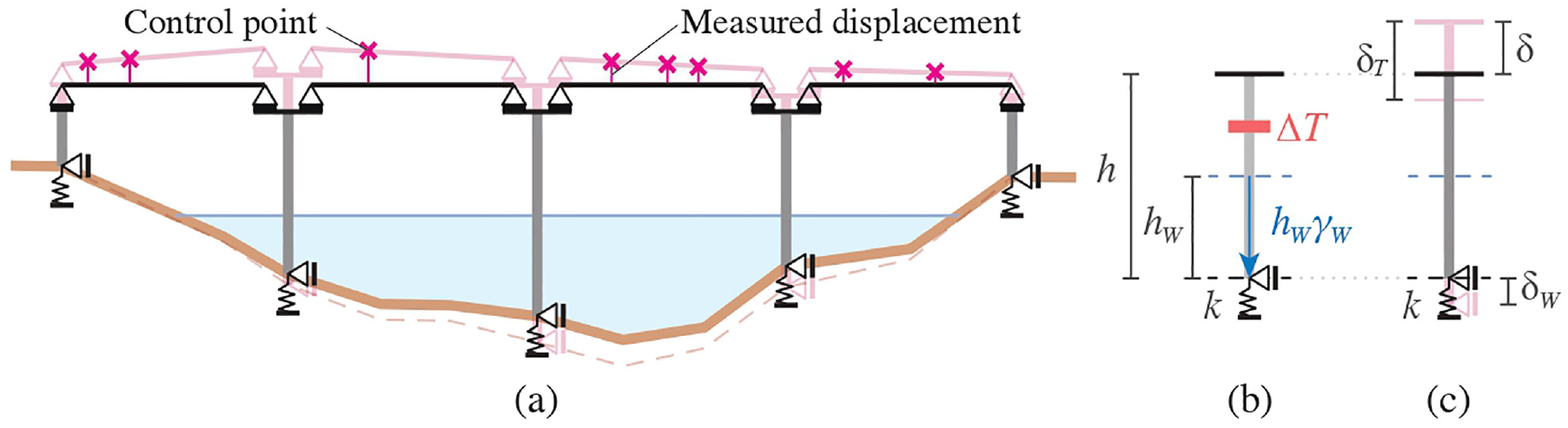
Simulated bridge model: (a) bridge scheme, (b) scheme of one pier and environmental actions and (c) Pier deformation.
where
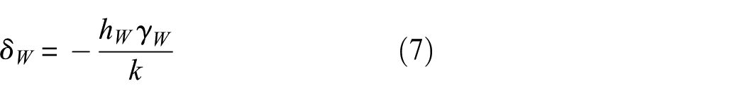
in which
The two contributions described above were then combined to provide the total displacement observable on top of the pier due to temperature and water level drivers:

The displacements obtained from InSAR data pertain to specific points on the bridge, which may either be PSs or control points that aggregate information from multiple PSs (i.e., the case considered in this study). Consequently, the final displacements of the control points (CP) used in the following analyses were derived as the linear combination of displacements from two consecutive piers (i.e.,
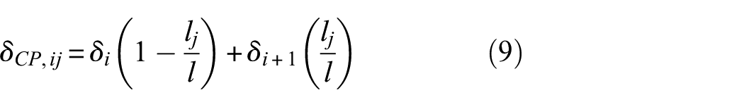
in which
Figure 10 compares real and simulated data of bridge B1 (and B1s) in time interval I1. Noteworthy, both temperature-driven oscillations and the negative peaks due to high water levels are qualitatively similar.
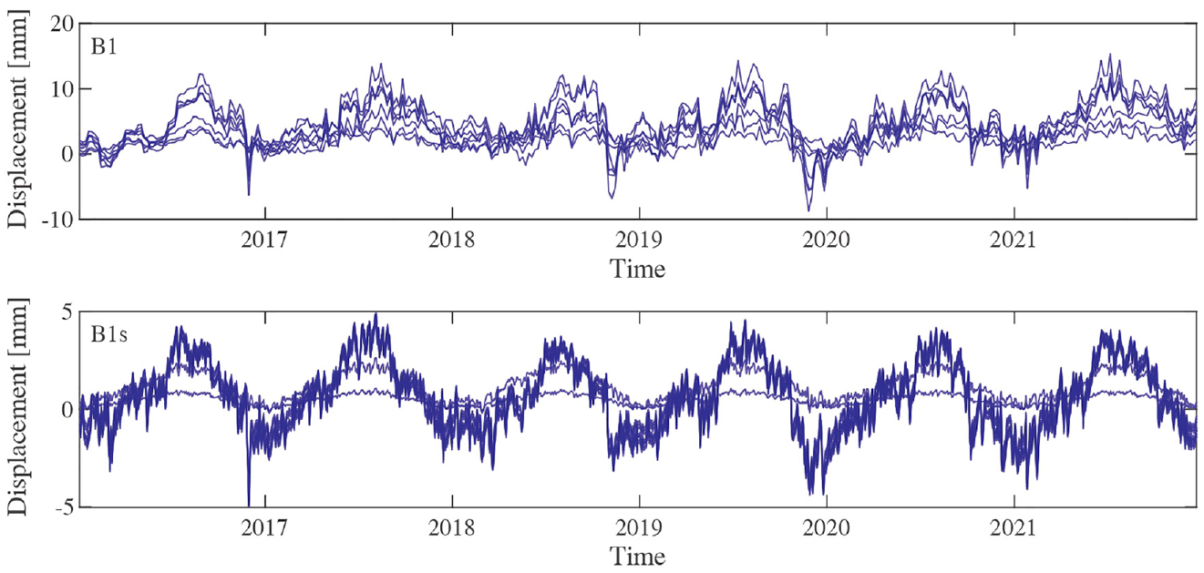
Time histories of the recorded displacements of B1 (top) and simulated displacements of B1s (bottom).
Modeled anomaly scenarios
As mentioned earlier, four distinct anomalous scenarios were simulated to test the procedure, namely, Sc, Se, Ou, and Up.
For the scouring effect (Sc), a temporary decrease in the support stiffness at the base of in-water piers was simulated. Specifically, the reduction was assumed to be proportional to the scouring depth, governed by the following relation:

where
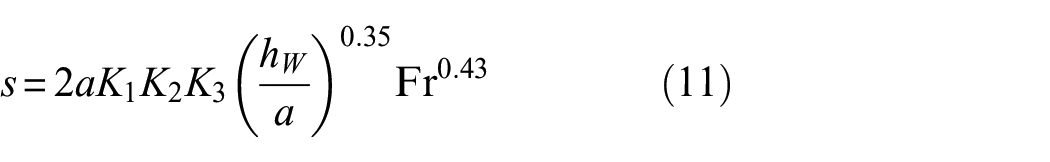
in which
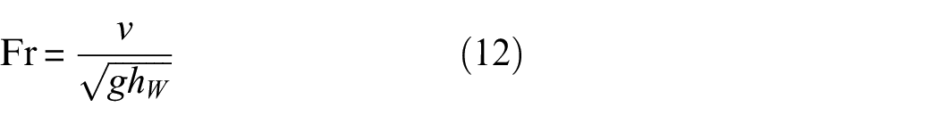
where
In this simulation, the pier width was considered the same for all bridges, with
For other anomalies, simpler modeling approaches were employed. Settlements (Se) and uplifts (Up) were simulated by vertically displacing the base of a single pier of the bridges downwards or upwards by 4 mm, respectively. Conversely, for outliers (Ou), the displacement of a single control point was shifted (upward or downward) by 4 mm. These displacement levels were selected to be realistically observable, given the millimeter-level accuracy of the real displacement datasets. 49
Figure 11 shows a timeline of the simulated anomalies for the modeled bridges. Notably, simulated anomalies appear and disappear over time, that is, with no permanent effects on the structures. While this approach may not reflect real-world scenarios, it is useful to validate the methodology. Specifically, it is assumed that bridge B1s underwent all four types of anomalies (identified through visual inspections), and the relevant datasets were labeled. Furthermore, B1s, B2s, and B5s experienced scouring due to a significant flooding event at the end of November 2019. Other simultaneous anomalies occurred between September and October 2020, during which B6s underwent uplift, while an outlier affected the data of B2s. Similarly, between September and November 2021, B4s and B7s experienced settlement and uplift, respectively.
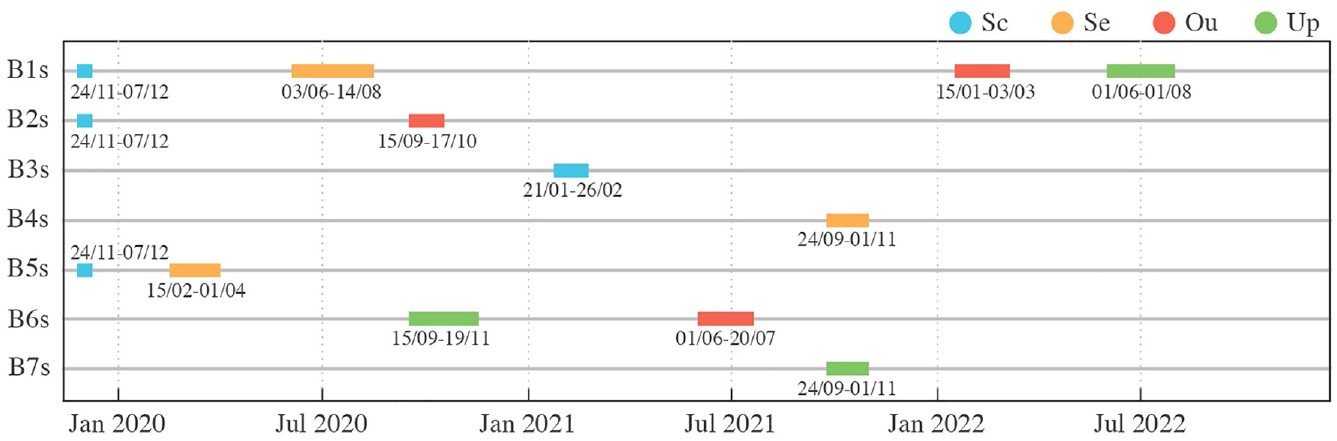
Timeline of simulated anomalies (dates in the format DD/MM).
Figure 12 displays the data instances of simulated bridges between April 2 and June 30, 2020. As expected, the projected features of bridge B1s (affected by a settlement in a part of the considered interval) deviate from the centroid, demonstrating the effectiveness of the proposed anomaly index.
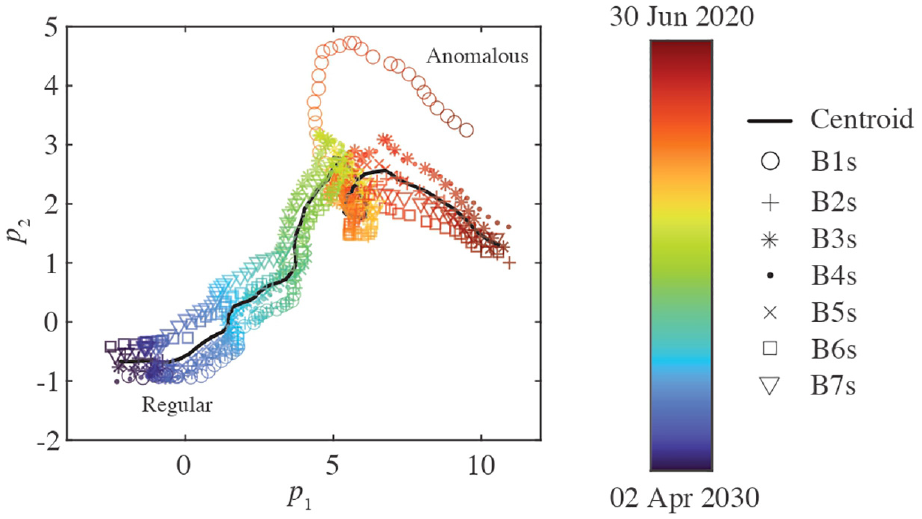
2D representation of the simulated data in the latent domain between 2 April and 30 June, 2020.
Anomaly detection and characterization
The methodology proposed in the article was applied to the simulated datasets to evaluate its ability to detect the modeled anomalies. During the initialization phase, reference data from January 5, 2016 to November 13, 2019 (a period without simulated damage) was employed to build the projection matrices and establish the anomaly detection threshold. This threshold was set as the highest 99th percentile of the relative distance between all bridges and the centroid.
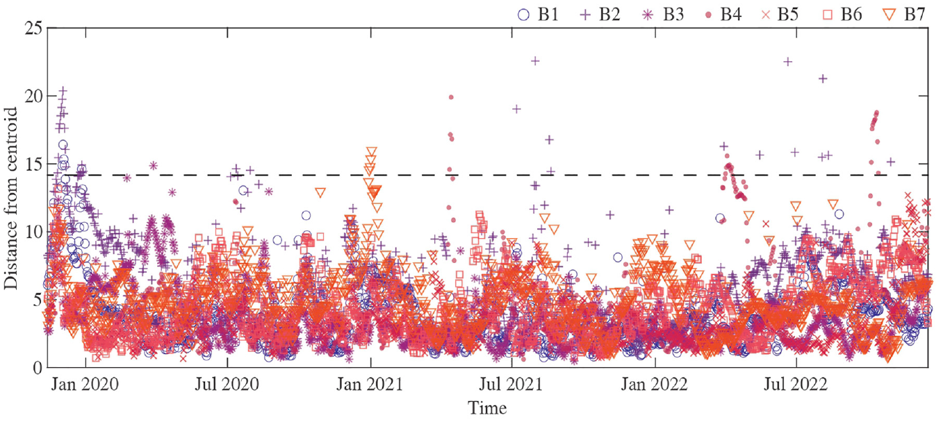
Subsequently, the anomaly index was computed for the monitoring interval (from November 13, 2019 to December 17, 2022). The resulting outcomes are presented in Figure 13, where data points exceeding the threshold (indicated by the dashed horizontal line) are identified as anomalies. Noteworthy, most anomalies were successfully detected, with the index associated with scour particularly prominent. Specifically, the true positive rate (TPR), representing the proportion of instances exceeding the threshold during simulated damage, is 59.05%. Conversely, the false positive rate (FPR), which measures the proportion of instances above the threshold when no damage was simulated, is 1.31%. The relatively low TPR should be ascribed to the oscillations of the damage index within the anomalous intervals driven by the inherent variabilities of the environmental input. Nonetheless, as shown in Figure 13, clusters of positive data are clearly identifiable for all simulated anomalous events, proving the capabilities of the method to detect anomalous bridge conditions. Additionally, the low FPR reflects the low occurrence of false alarms.
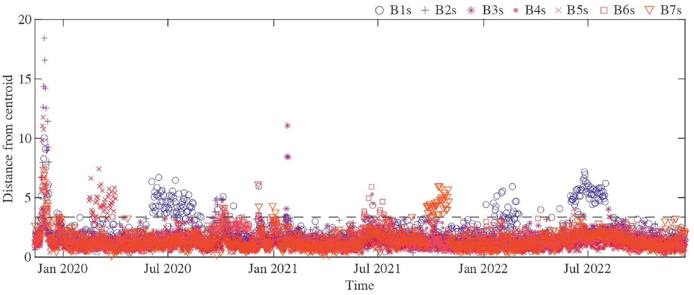
Anomaly index calculated over the analyzed time interval for the simulated bridges.
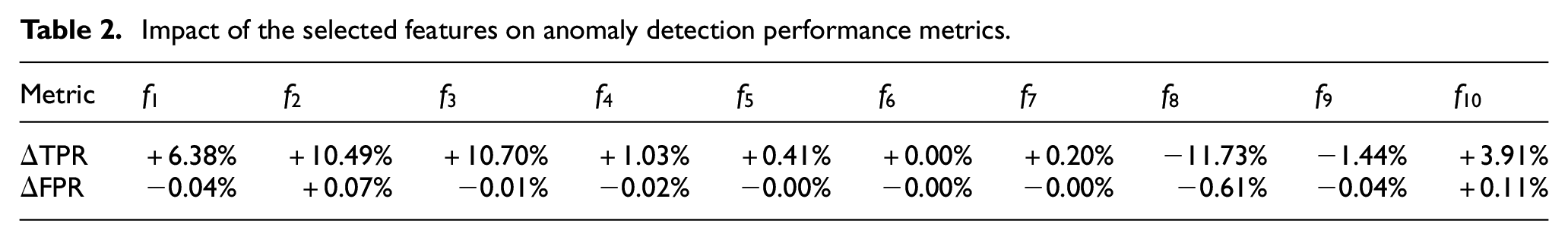
The impact of each selected feature on the performance indices has been evaluated by recalculating the TPR and FPR after removing one feature at a time from the analysis. The effect of each feature on the TPR and FPR is reported in Table 2. Specifically, the mean (
Impact of the selected features on anomaly detection performance metrics.
The instances of B1s in the monitoring interval were then employed to train a SOM with
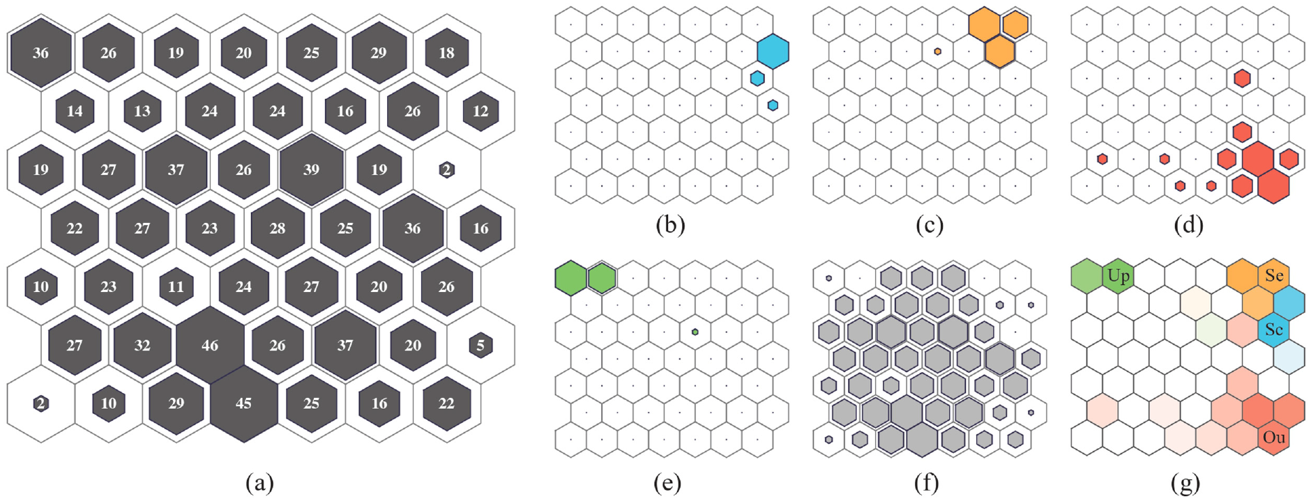
Data clustering for bridge B1s using the SOM: (a) distribution of data instances in the identified feature regions; distribution of data selected in the intervals, (b) 24 Nov 2019–07 Dec 2019, (c) 03 Jun 2020–14 Aug 2020, (d) 15 Jan 2022–03 Mar 2022, (e) 01 Jun 2022–01 Aug 2022, (f) the other time intervals and (g) cluster labels.
By feeding the SOM with different subsets of known anomalous instances, the regions to which they are assigned can be labeled accordingly. Specifically, Figure 14(b) to (e) depicts the classification outputs of the modeled anomalies, while Figure 14(f) illustrates the regions occupied by the remaining “regular” data. It is interesting to note that the Sc, Se, and Up data populate distinct regions that are well separated from the regular data. Conversely, Ou occupies a broader portion of the feature space and, in some areas, overlaps with the regular data. Figure 14(g) provides a synthesis of the obtained clusters, wherein the colors representing different anomalies have an intensity inversely proportional to the quantity of regular data that populate the regions.
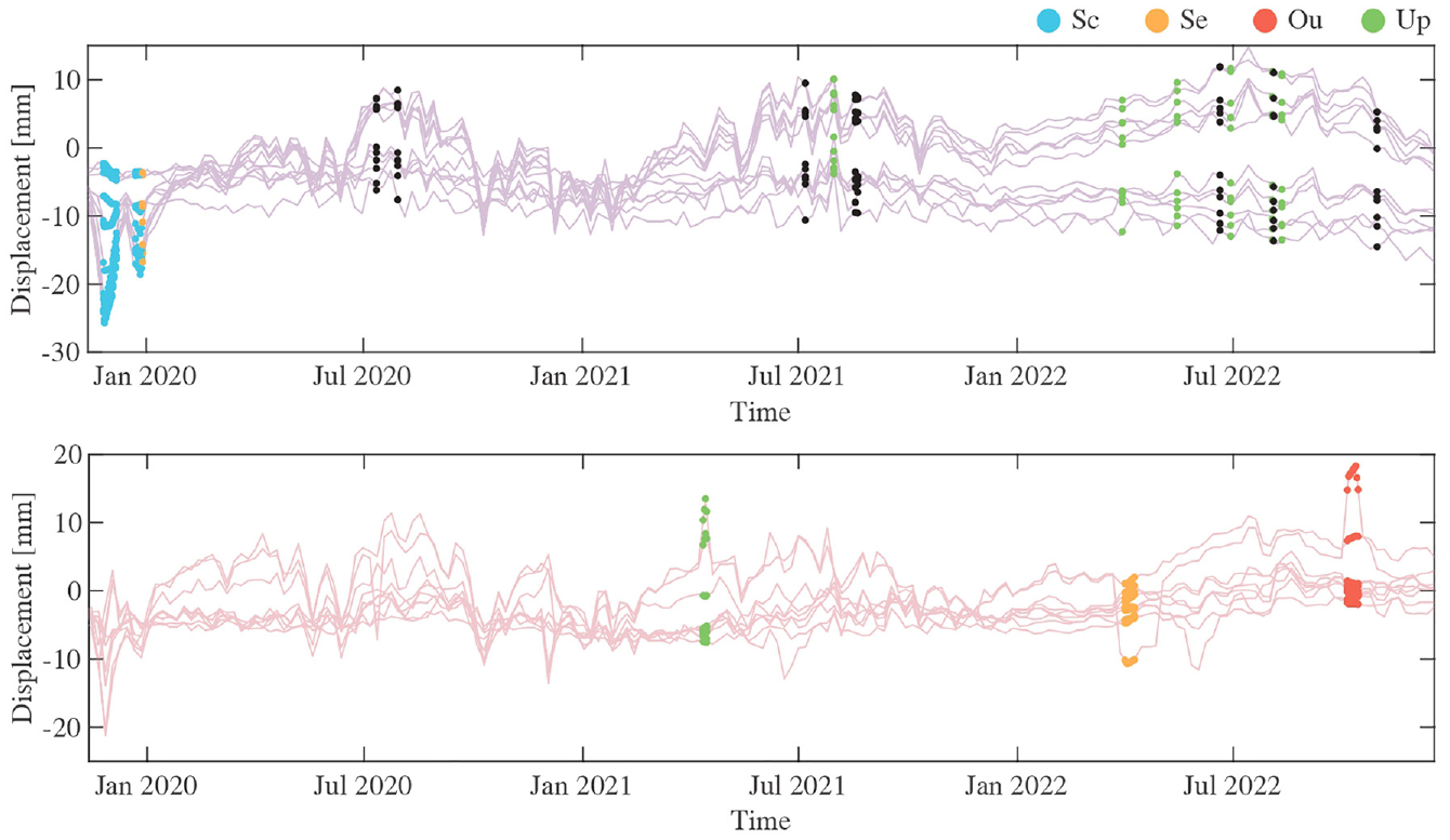
Figure 15 provides an overview of the classification outcomes resulting from inputting all available data into the SOM trained with B1s data. In this diagram, colored circles represent data instances allocated to regions assigned with the relevant labels. The circle size corresponds to the color intensity in Figure 14(g). Additionally, black points denote anomalous data (i.e., exceeding the anomaly threshold) that were not categorized within any known labeled regions. These data may indicate false alarms or unknown anomalies. In these cases, visual inspections could be arranged to assess the affected structures and potentially assign new anomaly labels.
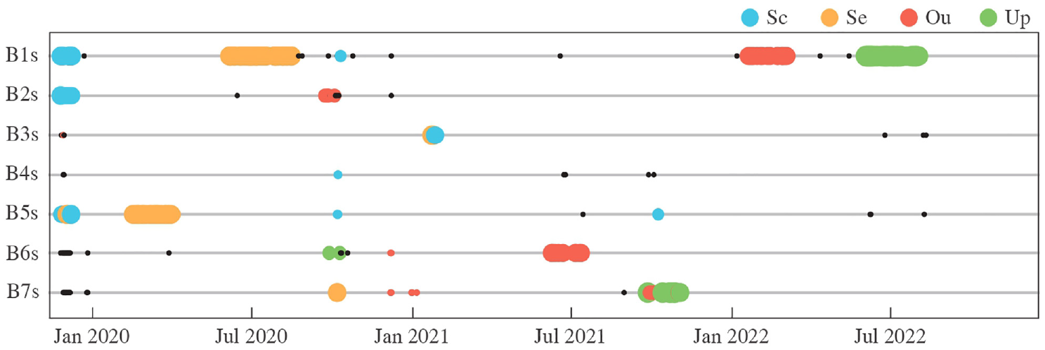
Classification of simulated data over the analyzed time interval.
The results indicate successful detection and characterization of all simulated anomalies based on B1s labels, with the exception of bridge B4s during simultaneous anomalies in B7s. Additionally, a higher incidence of false alarms is observed when concurrent anomalies manifest, such as those occurring at the end of November 2019, in September–October 2020, and in September–October 2021. This can be attributed to the method used to determine the centroid, which excludes only one bridge from the calculation, assuming the realistic scenario of only one structure experiencing anomalies at a time. Furthermore, most false alarms remain unassigned to known labels or fall within regions also populated by regular data.
Simulation-to-real knowledge transfer
The same procedure, conducted within analogous reference and monitoring time intervals, was applied for anomaly detection using real data collected from bridges B1–B7. In this case, the data were projected onto the source subspace of B1s, that is, the simulated bridge used as the source of information in the previous section. The link that allows projecting real data onto the simulated source domain and inferring anomaly information from it relies on the shared geometric characteristics and common environmental drivers (with comparable correlation coefficients) between the real and simulated configurations.38,66
Figure 16 illustrates the anomaly index obtained over the monitoring time interval. Prominent peaks above the threshold were identified at the end of 2019 for bridges B1 and B2, while B2 exhibited a persistently high index throughout 2022. Additionally, short-term anomalies were detected for B3, B4, and B7, all of which were temporary.
Anomaly index calculated over the analyzed time interval for the real bridges.
Obtained results for anomaly classification are summarized in Figure 17. While specific ground truth information for the analyzed bridges is unavailable, the classification labels suggest that the feature sets closely resembled those obtained in simulated scenarios during the identified anomalous intervals. Specifically, the anomalous events identified for bridges B1 and B2 at the end of November 2019 were classified as scour. Notably, monitoring agencies operating in the region of the Po River reported severe flooding events during that period, 67 which is also evident from the plot of water discharge in Figure 3. ARPAE documented a significant flood event from November 22 to December 3, 2019, characterized by hydrometric levels exceeding “level 3” in all main sections of the river. In the ARPAE monitoring portal, “level 3” signifies the occurrence of an exceptional flood involving extensive erosion and sediment transport phenomena. The event was caused by a rainfall that persisted from November 21 to November 25, lasting 120 h. Additionally, contributions to the flood were observed from snow melting in the Alps preceding and during the event.
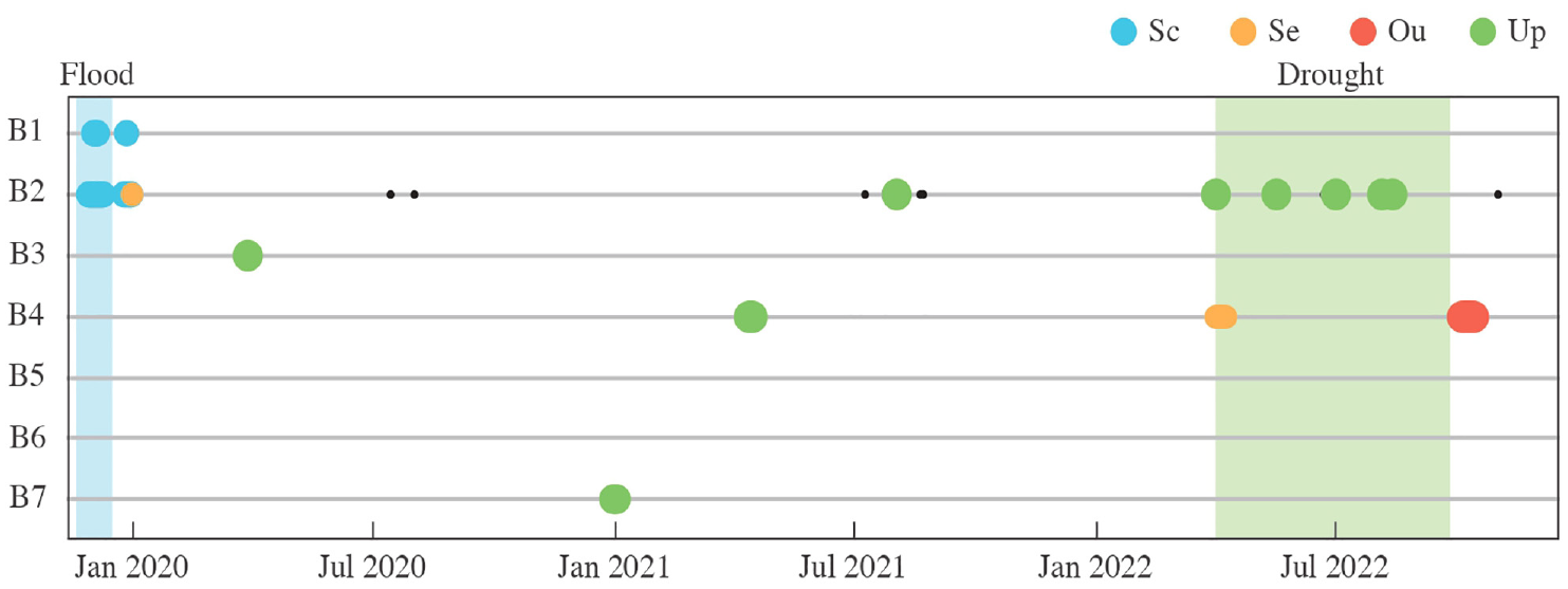
Classification of real data over the analyzed time interval. The highlighted intervals represent documented severe flood and drought events.
Moreover, the recurrent anomalies identified for B2 in 2022 were classified as uplift. This phenomenon is more noticeable during summer, coinciding with certified severe drought conditions in the region. 68 Specifically, this event led to an average river flow approximately 30% lower than the second-worst historical scenario ever recorded, an occurrence estimated to happen approximately once every 600 years. The prolonged drought may have contributed to the uplift observed in the riverbed near B2 during this period. 69
Other anomalies identified in the other bridges were shorter in duration and primarily categorized as uplift, settlements, and outliers.
Due to the black-box nature of the SOM and the lack of intuitive physical meaning for the projected features, it is challenging to identify in advance which specific measurement combination leads to a particular classification result. To help interpret the results, Figure 18 shows the displacement time histories of B2 and B4, with highlighted intervals corresponding to anomalous events indicated by the relevant label colors. As expected, data labeled as scour exhibit a significant downward displacement of some CPs within the river section. On the other hand, the uplifting event is characterized by a relative displacement of approximately 2 cm upward in some CPs with respect to the rest.
Displacement time histories of bridges B2 and B4 for interpretation of the assigned labels.
B4 also exhibits a brief period of uplift alongside instances of settlement and an outlier. While limited information is available for the identified uplift event, both the settlement and outlier anomalies appear to affect only a single control point. Consequently, both anomalies likely represent outlier occurrences. However, only the event at the end of 2022 is successfully classified as an outlier. In the anomaly identified in the first half of the year, the impact of the anomalous CP on statistical features might be comparatively lower than that used during the labeling process for outliers. Furthermore, the settlement label is justified by the downward shift of the anomalous CP. It is noteworthy that although the uplift event was identified for displacements similar to those of the outlier event, it was not labeled as an outlier, likely due to more than one CP displaying visibly anomalous displacements.
Conclusion
This article introduced a novel methodology for detecting and classifying anomalies across multiple bridges within a geographical area using satellite-based InSAR data and environmental measures. The proposed method employs SA to harmonize bridge features, enabling the detection of anomalies based on changes in their relative behaviors. This approach changes the paradigm of traditional SHM for bridges, which typically relies on comparing each structure with itself from the past.
Simulated results underscore the feasibility of the proposed procedure, although challenges may arise when anomalies occur in multiple bridges simultaneously. These findings highlight areas for further investigation in future studies with a more advanced definition of the data centroid and anomaly threshold. Nevertheless, the simple methodology employed in this study demonstrates the potential of the proposed strategy.
Furthermore, the study investigates the transferability of knowledge acquired from simulated data to real-world bridge monitoring scenarios. The same alignment method used to minimize differences between real bridges is applied to reduce discrepancies between simulated and real data. By projecting real data onto the feature subspace of simulated bridges, the method attempts to classify real instances using simulated labels, yielding promising results. Notably, detected anomalies in real data align with documented instances from previous studies and technical reports.
Overall, the proposed approach has significant practical benefits for bridge monitoring agencies. It offers a cost-effective means of anomaly detection and characterization, leveraging free data. This approach can be integrated into strategies to enhance the resilience and safety of transportation infrastructure. Additionally, given the rapid advancements in satellite and data acquisition technologies, measurements with improved frequency and spatial resolution will soon become available, thereby further enhancing the potential of the regional-scale monitoring methodology outlined in this study.
Footnotes
Declaration of conflicting interests
The author(s) declared no potential conflicts of interest with respect to the research, authorship, and/or publication of this article.
Funding
The author(s) disclosed receipt of the following financial support for the research, authorship, and/or publication of this article: Part of this study was carried out within the MOST—Sustainable Mobility National Research Center and received funding from the European Union Next Generation EU (PIANO NAZIONALE DI RIPRESA E RESILIENZA (PNRR)—MISSIONE 4 COMPONENTE 2, INVESTI MENTO 1.4—D.D. 1033 del 17/06/2022, CN00000023). Part of this study was carried out within the SAT4SHM project —“Quantifying the effects of Structure-Soil-Structure interaction on structural modal parameters by combining Earth observation data with on-site dynamic monitoring: an enhanced vibration-based Structural Health Monitoring approach”—funded by European Union, Next-Generation EU within the PRIN 2022 PNRR program (D.D.1409 del 14/09/2022 Ministero dell’Università e della Ricerca). This manuscript reflects only the authors’ views and opinions, and the Ministry cannot be considered responsible for them.