Impact time history reconstruction using dynamic weighted graph neural network under sensor fault situations

Abstract

This article introduces a dynamic weighted graph neural network (DWGNN) for precise reconstruction of impact force time histories under both fault and nonfault conditions in sensor networks. The DWGNN model integrates a one-dimensional convolutional neural network for extracting features from sensor signals and a graph neural network that dynamically adjusts its weight matrix based on node feature similarity, thereby reducing the impact of faulty sensor signals. Incorporating physical constraints, such as the distances between impact and sensor locations, improves the model’s performance. This innovative approach enables the accurate reconstruction of impact forces using only nonfaulty training data. Experimental validation on a stiffened metal plate, with mixed artificially generated and real measured signals, demonstrates the DWGNN model’s high accuracy and robustness. Data augmentation with fault signals significantly enhances the model’s accuracy under challenging fault conditions, proving the DWGNNs potential for real-time structural health monitoring and fault diagnosis in complex engineering structures.

Keywords

Impact force reconstruction graph neural network sensor fault dynamic weighted graph physics-informed constraint

Introduction

Impact force identification, which aims to locate and reconstruct the force history of an impact event,¹ is crucial in the field of structural health monitoring.² It provides valuable information for assessing damage and planning maintenance of structures such as bridges, buildings, and aircraft. However, this task is challenging due to complexities such as sensor noise, sensor failure, and unknown impact locations. While many traditional methods, regularization methods,^3–6 basis function methods,^7–9 and iterative methods,^10–12 have addressed the time history identification problem under known impact locations or complex model characteristics. However, it is foreseeable that when the impact location is unknown or the structural characteristics of the model are complex, the transfer functions between the impact location and sensors become either unavailable or highly inaccurate. Consequently, under circumstances where both the transfer function matrix and the impact load are unknown, most traditional methods proposed in the literature seem incapable of simultaneously and consistently solving both the localization and impact load history reconstruction problems using linear governing equations. To the best of our knowledge, only a few methods have been developed to address these challenges. However, they often rely on prior knowledge and assumptions to constrain the problem for numerical solutions. For instance, they may assume that the impact load originates from one of several candidate locations and that the spatial distribution of the impact locations shares the same characteristics (e.g., sparsity) as the excitation signals.^13–17

With the recent advancements in deep learning, neural networks have demonstrated significant potential in the field of force identification, particularly when traditional methods face challenges. Data-driven neural network approaches, such as convolutional neural networks (CNN) and recurrent neural networks (RNN), utilize sensor signals as input and produce force time histories or impact locations as output. These networks can learn complex transfer function relationships from sensor signals. For instance, Zhou et al.¹⁸ used a deep RNN for impact force identification on composite plates. Chen et al.¹⁹ developed a convolutional-recurrent encoder–decoder neural network determine the impact force’s position as well as its temporal history. Yang and Jiang²⁰ proposed a deep dilated convolution neural network for the purpose of dynamic force reconstruction. Zhou et al.²¹ introduced a gated temporal convolutional network-based method for impact force identification, capable of both localizing and reconstructing impact forces. While these data-driven methods show promise, they often struggle with handling complex spatial relationships and can be sensitive to sensor faults and noise. Wang et al.,²² based on the ultrasonic automatic diagnosis method enhanced by continuous wavelet transform and transfer learning deep convolutional neural network, evaluated the compression damage of concrete specimens under temperature changes and achieved good results.

Recently, graph neural networks (GNNs) have emerged as a powerful tool for modeling complex relationships in structured data. Unlike traditional data-driven neural networks, GNNs can naturally incorporate spatial information by representing the problem as a graph, where nodes and edges capture the relationships between different entities. This makes GNNs particularly well-suited for tasks involving irregular data structures and spatial dependencies, such as those found in structural health monitoring. For example, Li et al.²³ introduced multireceptive field graph convolutional networks for machine fault diagnosis, demonstrating enhanced accuracy. Qiu et al.²⁴ developed a denoizing GNN-based method for hydraulic component fault diagnosis, improving noise resilience. Atkinson et al.²⁵ applied convolutional GNNs for anomaly detection, highlighting their effectiveness in identifying anomalies in complex systems. Tsialiamanis et al.²⁶ explored GNNs in population-based Structural Health Monitoring (SHM), showing promising results in data-driven engineering applications.

In our previous work,²⁷ we leveraged GNNs for impact force localization and reconstruction, demonstrating their effectiveness in addressing some of the limitations of purely data-driven models. Unlike purely data-driven neural network models, our GNN is more model-driven with a graph structure.²⁸ When nodes and edges in the graph are assigned specific features, they can be utilized in neural network computations. In the Distance-assisted Graph Neural Network (DAGNN) model, the relationships between graph node features are associated with real physical distances, enabling the DAGNN model to learn from both the spatial and temporal information of dynamic structural responses. However, as the DAGNN model is applied to more complex and practical conditions, several architectural issues arise. The fixed window length for truncating sensor signals and the fixed admittance matrix for quantifying the graph structure in DAGNN simplify feature extraction and exchange, making it less adaptable to increasingly complex working conditions.²⁹

Furthermore, due to complex working environments, sensors often experience faults caused by external factors, leading to partial or complete loss of functionality.³⁰ These fault signals are often buried in massive data, making detection difficult. If faulty sensor signals are used without corrective measures, they can cause significant problems in sensor-based information systems.^31,32 Currently, there is limited research on impact force identification under sensor fault conditions, although it is a practical and meaningful issue. Due to its simple and fixed architecture, the DAGNN model cannot effectively identify faulty sensor signals or reconstruct impact force under sensor failure conditions.

Therefore, this work hope to propose a GNN-based model named dynamic weighted graph neural network (DWGNN) to reconstruct the time history of impact force in both nonfault and fault conditions in sensor networks, even without the presence of fault signals in the training dataset. Compared to the DAGNN model, the DWGNN model replaces the fixed window operation with a one-dimensional convolutional neural network (1D-CNN) to extract features from sensor time signals, and a GNN equipped with a weight matrix that dynamically adjusts in response to different fault situations. The weight matrix of the GNN is calculated by the similarity between node features, enabling the model to adapt to different fault situations. Additionally, the inclusion of the fault signal in the training dataset, achieved via data augmentation, can substantially enhance the recognition accuracy of the DWGNN model under extreme fault conditions.

The rest of this article is organized as follows. “Methodology” section gives the architecture of the DWGNN model for impact force time history reconstruction. In “Experiment validation” section, experiments are carried out on stiffened metal plates to verify the generalization ability of DWGNN. In “Time history reconstruction results with nonfaulty training signals” section, the results of time history reconstruction using the trained DWGNN model are given, and different unknown impact positions are analyzed. “Time history reconstruction results with faulty training signals” section discusses the time history reconstruction results of DWGNN model for various fault conditions when the training dataset contains fault sensor signals. “Conclusion” section draws some important conclusions.

Methodology

The aim of this section is to mathematically analyze the computational process of the DWGNN. Specifically, it examines how DWGNN uses acceleration sensor signals as input and load time histories as output, achieving accurate reconstruction of impact forces using only nonfaulty training data. To provide a more intuitive explanation of the DWGNN model architecture, the primary modules and their corresponding sections are illustrated as shown in Figure 1.

Figure 1.

Analysis of the computational process of DWGNN.

“The governing equation for force identification” section covers signal acquisition, detailing the collection of acceleration sensor signals and force hammer signals. “Types of sensors fault” section addresses common sensor fault types, presenting and analyzing the impact of four types of sensor faults on acceleration signals. “One-dimensional convolutional neural network feature extraction” section focuses on the 1D-CNN, which extracts features from time-domain acceleration signals. “Dynamic weighted graph construction” section discusses the construction of dynamic weighted graph structure, where time-domain features are analyzed for similarity and assigned weights. Finally, “Architecture of DWGNN model” section delves into GNN computation, which is used to reconstruct the impact force time histories.

The governing equation for force identification

For simplicity of description, a 2D stiffened metal plate is shown in Figure 2. It is evident that impact-induced signals are measured by $N$ sensors $S_{i}$ ( $i = 1, 2, . . ., N$ ) placed at certain locations ${PS}_{i} (x, y)$ on the plate. The sensor signal data vector refers to the vector representation of the measured data. However, due to the sensors in the real situation often have various unknown faults and errors, the measured sensor data $S_{i}$ is also uncertain. Thus, the primary issues addressed in this study are how to assess the accuracy of the uncertain sensor, how to carry out the reconstruction of the impact force time history $\hat{F}$ , and how to localize the impact position $P_{F} (x, y)$ . The force in this case is the single-source impact force that the force hammer inducts, and the measured data are vectorized and designated as the force signal data vector $F$ . These vectorized data are utilized as the model’s comparative samples.

Figure 2.

Impact force identification of 2D stiffened metal plate structure with uncertain sensors.

The following is the governing equation of force identification in the time domain for the system indicated above in Figure 2:

[P_{F} (x, y), \hat{F} (t)] = Ω^{S, F} [P_{S} (x, y), S (t)]

(1)

| \hat{F} (t) - F (t) | < ε

(2)

where $P_{F} (x, y)$ , $P_{S} (x, y)$ , $F (t)$ , $\hat{F} (t)$ , $S (t)$ , $ε$ are the impact location, sensor location, time history of the true impact force, time history of the reconstructed impact force, uncertain sensor signal time history, and error between the two impact force time history, respectively. $Ω^{S, F}$ is the force-sensor transfer function, which is likewise unknown.

Types of sensors fault

In recent years, many scholars have categorized sensor faults based on the characteristics of sensor data in studies related to sensor fault classification. Sensor faults can arise from external or internal causes. External factors include environmental conditions such as temperature, humidity, pollution, and corrosion. Among the studies on sensor fault classification, Ni et al.³³ provided one of the most detailed analyses, classifying sensor faults based on data characteristics. They also compiled a comprehensive list of common sensor fault data, offering an in-depth analysis of fault types, durations, and impacts. This work provides valuable guidelines for future research.

Overall, sensor faults can be broadly divided into two categories: incipient (slowly developing) faults and abrupt (sudden) faults.³¹ For aircraft structures and operating conditions, Samara et al.³⁴ extensively discussed three types of abrupt faults: complete failure, bias failure, and snowflake noise. This article extends the discussion to include incipient failures, specifically drift faults. The “incipient fault” indicates that the sensor system is operating abnormally or in an unstable state.²⁹ While the sensor continues to function, the data it produces is inaccurate. The errors introduced by incipient faults may initially be small and slow-changing, but they gradually increase over time, potentially leading to severe failures if not addressed.

To comprehensively analyze sensor faults, this study considers four fault types: complete fault, bias fault, drift fault, and snowflake noise. Examples of these fault types, along with a comparison to correct sensor signals, are presented in Figure 3. To simulate realistic fault conditions, the following assumptions are applied in this study: (i) the four fault types occur randomly in any sensor, (ii) the duration of fault signals is arbitrary, reflecting the randomness of sensor faults, (iii) the maximum amplitude of the fault signals is set equal to the maximum value of the response signals to ensure a consistent evaluation of fault impact.

Figure 3.

Examples of: (a) Correct sensor signal, (b) complete fault, (c) bias fault, (d) drift fault and (e) snowflake fault.

Complete fault, as shown in Figure 3(b), is one of the most frequent faults in sensors, where a constant value takes the place of the sensor’s data value. Complete fault adopted in this work is mathematically expressed as follow:

{\tilde{Y}}_{i} = max (Y_{i})

(3)

where ${\tilde{Y}}_{i}$ is the fault sensor data of the error part, $max (Y_{i})$ is a maximum value of the original signal.

Bias fault, as shown in Figure 3(c), is mainly caused by the sensor suddenly receiving a bias current or voltage, resulting in a constant error between the sensor measurement and the true value. Bias fault is mathematically expressed as follow:

{\tilde{Y}}_{i} = Y_{i} + max (Y_{i})

(4)

where $Y_{i}$ is the original sensor data of the error part, ${\tilde{Y}}_{i}$ is the fault sensor data of the error part, $max (Y_{i})$ is a maximum value of the original signal.

Drift fault, as shown in Figure 3(d), meaning that the offset or gain parameter varies over time when the sensor’s performance deviates from the initial calibration formula. Drift fault is mathematically expressed as follows:

{\tilde{Y}}_{i} = Y_{i} + y_{i}

(5)

where $Y_{i}$ is the original sensor data of the error part, ${\tilde{Y}}_{i}$ is the fault sensor data of the error part, $y_{i}$ is a linear sequence with a minimum value of 0 and a maximum value of $max (Y_{i})$ , and the length of $y_{i}$ is the same as the length of the error part $Y_{i}$ .

Snowflake fault, as shown in Figure 3(e), is mainly caused by the sensor’s susceptibility to noise from the environment, hardware, and internal sources. The primary sources of internal noise are circuit components like amplifier noise and sensor noise. Artificial or external interference with the sensor circuit is the source of external noise. While noise is a typical occurrence in sensor data, anomalous noise can lead to issues with sensor signals by masking the underlying signal. In this article, random data with the same mean and variance as the true signal are set as snowflake noise. Snowflake fault is mathematically expressed as follows:

{\tilde{Y}}_{i} = {y_{i}}

(6)

where ${\tilde{Y}}_{i}$ is the fault sensor data of the error part, ${y_{i}}$ is a random sequence whose mean and variance are the same as the original sensor data of the error part $Y_{i}$ .

One-dimensional convolutional neural network feature extraction

One-dimensional-CNNs architectures are proposed to extract features and classify the raw time-resolved signals.³⁵ One-dimensional-CNN integrates the feature extraction, feature transformation, data fusion, and classification processes into a single framework while carrying out 1D convolution and dimensionality reduction procedures. It works mainly on two primary operations: convolution and pooling. The former is adopted to extract features from a given dataset, and the latter is adopted to lessen the number of parameters and introduce translation invariance.³⁶

Mathematically, the operation of a 1D convolution can be expressed as follows:

y_{conv} [i] = \sum_{k = 1}^{K_{size}} x_{in} [i + k] \cdot w_{conv} [k] + b_{conv}

(7)

where $x_{in} [i]$ is the input sequence, $y_{conv} [i]$ is the output sequence, $w_{conv} [k]$ is the convolution kernel of size $K_{size}$ , and $b_{conv}$ is the bias term. This operation slides the kernel across the input sequence, capturing local patterns essential for understanding changes in sensor features. Following the convolution, the max-pooling operation is applied to reduce the dimensionality while retaining the most significant information. The max-pooling operation can be expressed as follows:

\begin{matrix} z_{pool} [j] = max {y_{conv} [j \cdot st], y_{conv} [j . st + 1], . . ., y_{conv} [j . st] \\ + P_{size} - 1} \end{matrix}

(8)

where $z_{pool} [j]$ is the pooled put at position $j$ , st is the stride of the pooling operation, and $P_{size}$ is the pooling window size. Max-pooling selects the maximum value in each local region, offering benefits such as dimensionality reduction, translation invariance, and noise robustness. Together, the convolution and max-pooling layers enable the model to extract compact, robust features from raw sensor signals, which are then input into the GNN for dynamic weighting and fault-tolerant impact force reconstruction. These additions aim to enhance the understanding of the feature extraction process.

As shown in Figure 4, this article proposes a two-layer 1D-CNN architecture for feature extraction. For illustration, the first layer consists of two convolutional kernels with a size of 32 and a stride of 4, while the second layer comprises four convolutional kernels with a size of 16 and a stride of 4. The 1D-CNN takes the acceleration sensor signals $S_{i} \in R^{1 \times 20, 000}$ measured in the signal acquisition shown in Figure 3 as the inputs. It then applies two convolutional layers and two max-pooling layers, followed by the Rectified Linear Unit (ReLU) activation function, to enable the model to capture more complex and nonlinear patterns. Finally, it uses the adaptive average pooling layer to flatten the features of all channels, and outputs are the time-domain feature $Y_{i} \in R^{1 \times 1240}$ of each acceleration sensor signal.

Figure 4.

Proposed 1D-CNN architecture for feature extraction.

To demonstrate the feature extraction performance of the 1D-CNN more intuitively, the five groups of acceleration sensor signals in Figure 3 are separately input into the 1D-CNN, and the five groups of time-domain features are output as shown in Figure 5. The acceleration signals undergo feature extraction and dimension reduction simultaneously through two convolutional layers and pooling layers. Moreover, by using the average pooling layer instead of the traditional fully connected layer at the end, the 1D-CNN avoids overfitting and preserves the intuitive features of the signals, such as the rising edge, amplitude, and trend. It can be seen that the fault signals and the correct signals have obvious differences in the feature maps, which can help us to provide a basis for judging whether the signals are faulty or not from the perspective of the similarity between the time-domain features output by the 1D-CNN.

Figure 5.

Time-domain features of acceleration sensor signals: (a) Correct signal, (b) complete fault, (c) bias fault, (d) drift fault, and (e) snowflake fault.

Dynamic weighted graph construction

An undirected graph $G = (N, E)$ is created as illustrated in Figure 6 by abstract the force identification problem depicted in Figure 2. $N$ reflects both the cardinality $| N | = N$ and the set of nodes $N$ in the graph. The time-domain feature of the acceleration sensor signal obtained by the 1D-CNN output is the feature of each node, which is represented by a total of nodes. $E$ is the graph’s collection of edges, and every node is connected to every other node pairwise.

Figure 6.

The dynamic weighted graph construction of the system.

Therefore, according to graph theory, the original adjacency matrix $A \in R^{N \times N}$ calculated to represent the graph $G$ can be obtained as follows:

A = [\begin{matrix} 0 & 1 & \dots & 1 & 1 \\ 1 & 0 & \dots & 1 & 1 \\ ⋮ & ⋮ & ⋱ & ⋮ & ⋮ \\ 1 & 1 & \dots & 0 & 1 \\ 1 & 1 & \dots & 1 & 0 \end{matrix}]

(9)

where $A$ is a symmetric (0,1)-matrix with zeros on its diagonal. The matrix’s elements show whether or not pairs of vertices in the graph are adjacent. Therefore, as mentioned before, since all nodes are connected to each other pairwise, the off-diagonal elements of the matrix $A$ are all equal to 1.

It is noteworthy that the element values in the original adjacency matrix $A$ only characterize the abstract topological connection relationships between the nodes. However, as mentioned earlier, the difference in the features of the two nodes can be reflected by the edge connected between the two nodes. That is to say, the difference between time-domain sensor features $Y i$ can make the elements in the adjacency matrix $A$ not only have topological connection but also have more physical meaning. On the one hand, these differences are normal differences caused by different sensor layouts, and on the other hand, they are fault differences caused by a sensor failure.

Furthermore, this article first performs max-normalization on each group of time-domain features $Y$ separately, to reduce the similarity difference between acceleration responses caused by impact force with different amplitudes as follows:

{\bar{Y}}_{i} = \frac{Y_{i}}{max (Y_{i})}

(10)

Then, the Euclidean distance $M_{i, j}$ between each pair of normalized time-domain features $\bar{Y} i$ and $\bar{Y} j$ is calculated as follows:

M_{i, j} = ‖ {\bar{Y}}_{i} - {\bar{Y}}_{j} ‖_{2}

(11)

where the larger the Euclidean distance $M_{i, j}$ , the worse the similarity between the normalized time-domain features ${\bar{Y}}_{i}$ and ${\bar{Y}}_{j}$ . There are three commonly used methods for evaluating vector similarity: Euclidean distance, Manhattan distance, and cosine similarity. In this study, we used these methods to evaluate the similarity of the time-domain features extracted by the 1D-CNN, which is used as input for weight calculation. The goal of the weight calculation is to retain the correct information from the sensor’s time-domain features before a fault occurs and filter out the erroneous information after the fault happens. Based on this objective, we believe that Euclidean distance is the most interpretable and simple method among the three, for the following reasons: (i) While Euclidean distance has a higher computational complexity than Manhattan distance, it better preserves the relationships between time-domain features, and when anomalies occur, the squared term in Euclidean distance amplifies the effect of outliers, enabling more effective weight adjustment. (ii) Moreover, Euclidean distance offers a clear computational advantage over cosine similarity, which requires the calculation of vector magnitudes and dot products, significantly increasing the overall computational cost in neural network processing.

Thus, a Euclidean distance matrix $M$ can be obtained as follows:

M = [\begin{matrix} 0 & M_{1, 2} & \dots & M_{1, N - 1} & M_{1, N} \\ M_{2, 1} & 0 & \dots & M_{2, N - 1} & M_{2, N} \\ ⋮ & ⋮ & ⋱ & ⋮ & ⋮ \\ M_{N - 1, 1} & M_{N - 1, 2} & \dots & 0 & M_{N - 1, N} \\ M_{N, 1} & M_{N, 2} & \dots & M_{N, N - 1} & 0 \end{matrix}]

(12)

where $M$ is a symmetric matrix with diagonal elements being zero. It is noteworthy that when all sensors are normal, the similarity difference between the sensor time-domain features is mainly caused by different sensor positions. However, when a sensor fails, the similarity difference between the sensor time-domain features caused by the fault will be much greater than normal, making the nondiagonal element values of the corresponding row and column of the sensor much larger than the rest of the element values.

The upper triangular and nondiagonal elements of Euclidean distance matrix $M$ are extracted to form an upper vector $M_{s}$ as follows:

M_{s} = [M_{1, 2}, \dots, M_{1, N}, M_{2, 3}, \dots, M_{2, N}, \dots, M_{N - 1, N}]

(13)

where Softmax function is used to normalize the elements as follows:

\bar{M} = 1 - softmax (M_{S}) = 1 - \frac{\exp (M_{s})}{\sum \exp (M_{s})}

(14)

where the element values in $\bar{M}$ are between 0 and 1. Place the elements in $\bar{M}$ according to their original positions in the Euclidean distance matrix $M$ and form a new symmetric matrix $M \in R^{N \times N}$ as follows:

M = [\begin{matrix} 0 & {\bar{M}}_{1, 2} & \dots & {\bar{M}}_{1, N - 1} & {\bar{M}}_{1, N} \\ {\bar{M}}_{1, 2} & 0 & \dots & {\bar{M}}_{2, N - 1} & {\bar{M}}_{2, N} \\ ⋮ & ⋮ & ⋱ & ⋮ & ⋮ \\ {\bar{M}}_{1, N - 1} & {\bar{M}}_{2, N - 1} & \dots & 0 & {\bar{M}}_{N - 1, N} \\ {\bar{M}}_{1, N} & {\bar{M}}_{2, N} & \dots & {\bar{M}}_{N - 1, N} & 0 \end{matrix}]

(15)

From Equations (8)–(13), it can be assumed that when all sensors are functioning correctly, the Euclidean distances of all features in the matrix $M$ are similar, leading to nondiagonal elements of the matrix $M$ being less than, but close to 1. Conversely, in the event of a sensor fault, the Euclidean distance of the corresponding row and column in the matrix $M$ becomes abnormally large. This results in some rows and columns of the nondiagonal elements in the matrix $M$ becoming smaller than in the correct situation, significantly less than 1. Therefore, the nondiagonal element values in the matrix $M$ can be considered as the information validity values between the corresponding sensors. The matrix $M$ is referred as the dynamic weight matrix.

By dot multiplying the original adjacency matrix $A$ and the weight matrix $M$ , the information validity difference between the node features can be used as the specific representation of the edges, replacing the abstract topological relationship of matrix $A$ . The dynamic weighted adjacency matrix $\tilde{A}$ can obtained as follows:

\tilde{A} = A ° M

(16)

where $°$ is Hadamard product. Therefore, $\tilde{A} \in R^{N \times N}$ dynamically changes according to the acceleration time-domain signal of each group of sensors, which is the node time-domain feature.

Then, a dynamic weighted degree matrix $\tilde{D} \in R^{N \times N}$ is calculated as follows:

\tilde{D} = [\begin{matrix} \sum_{i}^{N} \frac{{\tilde{A}}_{1, i}}{N - 1} \\ ⋱ \\ \sum_{i}^{N} \frac{{\tilde{A}}_{N, i}}{N - 1} \end{matrix}]

(17)

where the element of $\tilde{D}$ on the graph $G$ denotes the total information validity weight between the node and the other nodes. By thoroughly taking into account the edges and the nodes as follows, a matrix $Δ \in R^{N \times N}$ known as the admittance matrix may be constructed using the dynamic weighted adjacency matrix $\tilde{A} \in R^{N \times N}$ and the dynamic weighted degree matrix $\tilde{D} \in R^{N \times N}$ :

Δ = \tilde{D} - \tilde{A}

(18)

In general, we obtain the node effective information weights by mapping the similarity based on the Euclidean distance of the temporal features output by 1D-CNN, which replaces the topological connection relationships between nodes in the graph structure and helps DWGNN perform better reconstruction under normal and fault data.

Architecture of DWGNN model

A three-layer DWGNN model can be proposed. The interaction layer is the first layer. This layer uses the dynamic graph structure, which includes the degree matrix $\tilde{D} \in R^{N \times N}$ and admittance matrix $Δ \in R^{N \times N}$ , as well as the time-domain features $Y \in R^{N \times 1240}$ that the 1D-CNN produced as inputs. Via the graph structure, each node feature propagates and trades information. The following is an expression for the first layer:

F_{I} = σ (\tilde{D} \cdot Y \cdot W_{11} + Δ \cdot Y \cdot W_{12})

(19)

where $σ (\cdot)$ denotes the activation function, and ReLU function is used in this article. $\tilde{D} \cdot Y \cdot W_{11}$ represents the effective information extraction of each node’s feature, and $Δ \cdot Y \cdot W_{12}$ represents the information exchange and propagation of the entire graph $G$ . $W_{11} \in R^{N \times hid}$ and $W_{12} \in R^{N \times hid}$ are two trainable weight matrices.

The second layer is a reconstruction layer. It reconstructs each node embeddings $F_{I} \in R^{N \times hid}$ output by the first layer into a force feature. The second layer is expressed as follows:

F_{G} = σ (\tilde{D} \cdot F_{I} \cdot W_{21} + Δ \cdot F_{I} \cdot W_{22})

(20)

where $W_{21} \in R^{hid \times 1245}$ and $W_{22} \in R^{hid \times 1245}$ are two trainable weight matrices. It is noteworthy that the output $F_{G} \in R^{N \times 1245}$ of the second layer should be the force feature reconstructed by each node. Therefore, by calculating a latent variable from the output $F_{G} \in R^{N \times 1245}$ and the degree matrix $\tilde{D} \in R^{N \times N}$ , a direct linear relationship can be established with the different distances of the sensors at the force impact time. We name this latent variable as the embedding distance $δ^{N \times 1}$ , as expressed follows:

δ = Mean (F_{G}) ○ Diag (\tilde{D})

(21)

where $Diag (\cdot)$ is the diagonal matrix’s transformation into a column vector, and $Mean (\cdot)$ is the average function applied to each row of the matrix. As was previously said, constraints are used to direct the model’s extraction of a latent feature that is associated to the actual physical distance $ρ^{N \times 1}$ between the impact position and the sensor location, giving the embedding distance $δ^{N \times 1}$ physical meanings. The linear correlation between $δ^{N \times 1}$ and $ρ^{N \times 1}$ is measured using the Pearson’s correlation coefficient, which can be written as follows:

pr = \frac{cov (δ, ρ)}{ς_{δ} \cdot ς_{ρ}}

(22)

where $cov (δ, ρ)$ is the covariance of $δ^{N \times 1}$ and $ρ^{N \times 1}$ . $ς_{δ}$ and $ς_{ρ}$ are the variances of $δ^{N \times 1}$ and $ρ^{N \times 1}$ , respectively. $pr$ is the ratio between $cov (δ, ρ)$ and the product of $ς_{δ}$ and $ς_{ρ}$ . As a result, the outcome $pr$ is always between −1 and 1.

The third layer of the DWGNN model takes the output $F_{G} \in R^{N \times 1245}$ of the second layer as the input, and fuses the reconstructed force features of each node. Finally, a time-domain impact feature vector $F_{O} \in R^{1 \times 1245}$ is output. The third layer can be expressed as follows:

F_{O} = σ (W_{3} \cdot F_{G})

(23)

where the graph’s node features are fused and decoded using the trainable weight matrix $W_{3} \in R^{1 \times N}$ .

Finally, $F_{O} \in R^{1 \times 1245}$ passes through two deconvolution layers to obtain the reconstructed force time history $\hat{F} \in R^{1 \times 20000}$ , where $F_{D} \in R^{1 \times 4993}$ is the intermediate force feature obtained by $F_{O} \in R^{1 \times 1245}$ after passing through the first deconvolution layer. The loss function is calculated with the comparative sample $F \in R^{1 \times 20, 000}$ as follows:

Loss = \frac{{‖ \hat{F} - F ‖}_{2}}{| pr |}

(24)

where the pr term is added as the denominator to the normal modified mean square error loss function between the reconstructed force time history $\hat{F}$ , and the comparative sample $F$ , to penalize the embedding distance with poor correlation to the physical distance. Finally, the DWGNN model’s weights are updated through the propagation of the loss back.

The DWGNN model flow graphic for impact force reconstruction is shown in Figure 7.

Figure 7.

The DWGNN model flow graphic.

As mentioned above, each group of time-domain sensor feature $Y$ can output the reconstructed force time history $\hat{F}$ through the DWGNN model and two layers of deconvolution layers.

Two new criteria are presented to assess the DWGNN model’s generalization performance quantitatively.

The total accuracy of the identification is measured by the relative error (RE) between the identified impact forces and the original impact, which is defined as follows:

RE = \frac{‖ F - \hat{F} ‖ 2}{‖ F ‖ 2} \times 100 %

(25)

where $F$ is the true impact force, and where $\hat{F}$ is the real impact force.

An essential tool in SHM for measuring the peak of impact force is the peak error (PE), which is defined as follows:

PE = \frac{| max (F) - max (\hat{F}) |}{| max (F) |} \times 100 %

(26)

Experiment validation

An experiment is carried out in this section to demonstrate the DWGNN model’s usefulness and applicability.

Experimental set-up

A rectangular metal stiffened plate is used in the experiment, which is made of aluminum alloy material. The plate’s left side is clamped by a stainless fixture to mimic a fixed boundary condition, while the other three sides are free boundary conditions, as seen in Figure 8(a). Two I-beams that cross the whole length of the plate are welded to the back of the plate structure, as seen in Figure 8(b). As shown in Figure 8(c), excluding the fixed part, the length of the plate is 60 cm, the width is 50 cm, and the thickness is 0.3 cm. The I-beam material is the same as the plate. The specific shape parameters of the I-beam are shown in the schematic diagram in Figure 8(d).

Figure 8.

Schematic diagram of the metal stiffened plate structure in the experiment: (a) real structure plate surface, (b) real structure stiffened beam surface, (c) schematic diagram of the plate surface, and (d) schematic diagram of the stiffened beam cross-section.

Dataset acquisition

As shown in Figure 8(a), the impact force is triggered and measured by an impact hammer, striking vertically on the metal stiffened plate structure. Six acceleration sensors are arranged on the plate structure to measure the vibration acceleration signal in the direction perpendicular to the plate surface.

The plate structure is divided into two regions A and B as shown in Figure 9(a): region A consists of 18 rectangular subregions, which are nonstiffened areas; region B consists of 12 rectangular subregions, which are stiffened areas. Acceleration sensors $S 1, S 2, S 3, S 4, S 5, S 6$ are arranged on $A 1, A 8, A 15, A 4, A 11, A 18$ , respectively, as shown in Figure 9(a). As seen in Figure 8(a), the applied impact force is recorded using an impact hammer that is coupled to a force sensor. After triggering 2 s, the laser vibrator PSV-500 records the force and acceleration signal at a 10 kHz sample frequency.

Figure 9.

Experimental dataset acquisition: (a) impact zone division and sensor placement points of plate structures, (b) training set and validation dataset acquisition points, (c) testing dataset acquisition points.

The training dataset and validation dataset are obtained by striking the center positions of regions A and B, or the positions indicated by pentagrams, a total of 30 positions, using an impact hammer, as seen in Figure 9(b). For every position, 21 impacts of varying amplitudes are performed. Every impact force has a random maximum amplitude that ranges from 20 to 200 N. As a result, the DWGNN model is trained using a training dataset of 600 samples, and it is fine-tuned using a validation dataset of 30 examples. Additionally, 78 additional testing impacts indicated by the triangles and the 30 impact positions for training are impacted again to form a testing dataset with 108 different impact positions, which includes almost the entire plate as shown in Figure 9(c). This is done in order to test the generalization performance and practicality of the proposed networks throughout the entire plate. One sample with a random force amplitude is collected for each testing impact position.

Dataset classification

This article explores the impact force identification results of the DWGNN model under various conditions, utilizing different datasets for training and testing as shown in Table 1.

Table 1.

Datasets and conditions in DWGNN model study.

Dataset	Condition	Samples	Description
Training dataset I	Nonfault	600	Experimental sensor signals collected.
Testing dataset I	Nonfault	108	Experimental sensor signals collected.
Testing dataset II	Fault	108	Adds a fault at a random time during the entire acceleration signal period to testing dataset I.
Testing dataset III	Fault	108	Adds a fault in the first 10% time period of the acceleration signal to testing dataset I.
Testing dataset IV	Fault	108	Adds a fault in the first 1% time period of the acceleration signal to testing dataset I.
Training dataset II	Fault	600	Adds the fault data that occurred in the first 1% of the time to training dataset I.
Training dataset III	Fault	6000	Increases Training dataset I to 10 times and adds the fault that occurred in thefirst 1% of the time.
Training dataset IV	Fault	9000	Increases training dataset I to 15 times and adds the fault that occurred in thefirst 1% of the time.

DWGNN: dynamic weighted graph neural network.

In the absence of faults, training dataset I and testing dataset I are employed, both derived from sensor signals as documented in “Dataset acquisition” section.

When considering fault conditions, faults are introduced into the signal of a randomly selected sensor to generate additional datasets. Three distinct fault occurrence conditions are examined: a fault occurring at a random time during the entire acceleration signal period (training dataset II, testing dataset II), a fault manifesting within the first 10% of the acceleration signal time period (testing dataset III), and a fault appearing within the initial 1% of the acceleration signal time period (testing dataset IV).

Furthermore, to examine the influence of the sample size on the DWGNN model when faulty sensor signals is included in the training dataset, training dataset I is augmented by factors of 10 times (training dataset III) and 15 times (training dataset IV), respectively.

Time history reconstruction results with nonfaulty training signals

In this section, the model training of the DWGNN by training dataset I will be discussed, as well as the effectiveness and accuracy of the time history reconstruction of the experimental metal stiffened plate structure with testing dataset I. In addition, the time history reconstruction results of the testing datasets II, III, and IV are also used to verify the performance of the DWGNN model under fault conditions.

Model training by nonfaulty training dataset I

After fine tuning, the hyperparameters and specific architecture of DWGNN is listed in Table 2. Moreover, the loss of the validation dataset at each epoch is compared with the prior epoch to avoid over-fitting. A multiplication of attenuation coefficient is applied to the present learning rate if the loss hovers above 10%. The model training is carried out using a GPU (NVIDIA RTX 4090 24 GB) device.

Table 2.

The hyperparameters and specific architecture of DWGNN.

Hyperparameters and architecture	DWGNN
Optimizer	Adam
Batch size	4
Hidden neuron count	1024
Maximum epoch	100
Learning rate	0.0001
Attenuation coefficient	0.7

DWGNN: dynamic weighted graph neural network.

The history of the training loss, validation loss, and learning rate of the DWGNN model are shown in Figure 10. The training loss of DWGNN converges quickly and smoothly without significant fluctuations. The same trend is also reflected in the validation loss, and the adaptive learning rate associated with it remains at 0.0001, indicating that no overfitting occurs. Therefore, it can be considered that DWGNN has been sufficiently and well trained.

Figure 10.

The training loss, the validation loss, and the learning rate of the DWGNN model with epoch.

Time history reconstruction results with nonfault testing dataset I

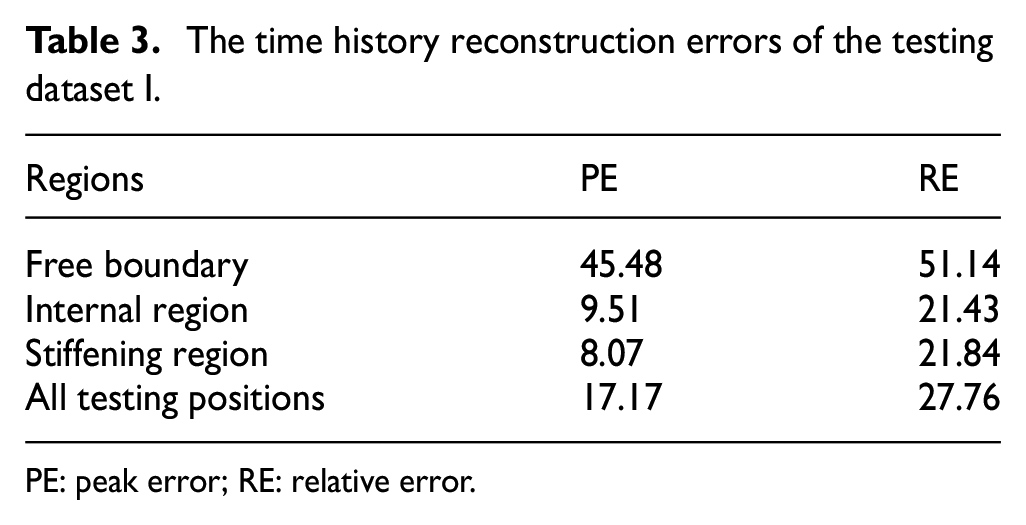
The testing dataset I was input into the trained DWGNN model to analyze its accuracy and generalization. In addition, to analyze the time history reconstruction results of different regions on the stiffened plate more intuitively and specifically, we divided the stiffened plate into three regions: free boundary, internal region, and stiffening region, and performed error statistics separately. As shown in Figure 11, the internal region is defined as the area 5 cm away from the 3 free edges, occupying 74% of the total plate area, with 85 impact positions. The remaining plate area is defined as the free boundary region, with 23 impact positions. The stiffening region is the stiffened part within the internal region, with 34 impact positions.

Figure 11.

Three regions divided on the stiffened plate structure: free boundary (①), internal region (② and ③), and stiffening region (③).

The time history reconstruction errors are listed in Table 3 and the nephograms of the reconstruction errors at different positions on the entire plate structure is shown in Figure 12. The rectangular area inside the blue dotted line is the internal region.

Table 3.

The time history reconstruction errors of the testing dataset I.

Regions	PE	RE
Free boundary	45.48	51.14
Internal region	9.51	21.43
Stiffening region	8.07	21.84
All testing positions	17.17	27.76

PE: peak error; RE: relative error.

Figure 12.

The nephograms of DWGNN with testing dataset I of (a) PE and (b) RE.

It can be seen that the DWGNN model achieved a very high reconstruction accuracy in the stiffening beam region, solving the nonlinear effect caused by the stiffening beam on the time history reconstruction of the plate structure. Therefore, it can be considered that the DWGNN model achieved a high reconstruction accuracy in the entire internal region, which is satisfactory.

However, the DWGNN model exhibited high reconstruction errors in the free edge region. Figure 12 illustrates that the three free edges, and the unclamped boundary parts shown in Figure 8(c), which means that the reconstruction error is higher. On the one hand, this is because the size and complexity of the plate make the acceleration response of the free edge more complex and more susceptible to external influences when vibrating, and this part of the data was not added to the DWGNN training dataset, making the DWGNN model not fully trained for the free edge vibration; on the other hand, although the DWGNN model added the real physical distance between sensor location and impact location as a constraint, this distance is constant and does not change according to the different boundary conditions, these two reasons reduce the generalization and robustness of the DWGNN model in the free edge recognition, which is also a current drawback of the DWGNN model. Therefore, the internal region on the plate structure is considered as the effective reconstruction region of the DWGNN model. Only the reconstruction results of the internal region will be discussed in the subsequent discussions.

Finally, the time history results reconstructed by a fine-tuned DAGNN model [27] are compared, as listed in Table 3. Typical time history reconstruction results for both the DWGNN and DAGNN models are shown in Figure 13, with the reconstruction error nephograms of the DAGNN model presented in Figure 14.

Figure 13.

The typical time history reconstruction results with the testing dataset I of: (a) DWGNN; (b) DAGNN.

Figure 14.

The nephograms of DAGNN with testing dataset I of (a) PE and (b) RE.

Table 4 indicates that the DWGNN model’s reconstruction error is about 5% lower than that of the DAGNN model. Additionally, the nephogram color distribution for the DWGNN model (Figure 12) is more uniform than that of the DAGNN model (Figure 14) in the internal region, especially in the upper left corner where the fixed support boundary is not comprehensive. This improvement is attributed to the DWGNN model’s use of 1D-CNN to extract features from the sensor acceleration time-domain signal, unlike the direct window truncation in the DAGNN model. The 1D-CNN convolutional operator not only extracts local features but also considers the overall characteristics of the acceleration time-domain signal.

Table 4.

The time history reconstruction results of DWGNN model compared with DAGNN model with testing dataset I.

Model	PE	RE
DWGNN	9.51	21.43
DAGNN	14.29	25.64

DWGNN: dynamic weighted graph neural network; DAGNN: Distance-assisted Graph Neural Network; PE: peak error;RE: relative error.

Time history reconstruction results with faulty testing datasets II, III, and IV

It can be inferred that the DWGNN model trained by training dataset I should be unfamiliar with various fault signals in the testing datasets II, III, and IV. As mentioned in “One-dimesional convolutional neural network feature extraction” and “Dynamic weighted graph construction” sections, the dynamic weight matrix $M$ of one group of acceleration signals can be obtained by Equations (6)–(8).

Furthermore, to demonstrate illustrate the effectiveness of the weight matrix $M$ for all sets in testing dataset. The skewness criterion in statistics is used to quantify the distribution of nondiagonal elements in the $M$ matrix. First, extract the nondiagonal elements in the weight matrix $M$ corresponding to the 108 sets of testing dataset to form the vector $\tilde{M} \in R^{1 \times 3240}$ . The skewness value of the $\tilde{M}$ is calculated as follows:

Skew = \frac{\frac{1}{3240} \sum_{i = 1}^{3240} {({\tilde{M}}_{i} - Mean (\tilde{M}))}^{3}}{{(\frac{1}{3240} \sum_{i = 1}^{3240} {({\tilde{M}}_{i} - Mean (\tilde{M}))}^{2})}^{\frac{3}{2}}}

(27)

In this article, a negative skewness value for the matrix $M$ indicates a bias toward 1 among its elements. This suggests that the weight values of each node are similar, implying full utilization of each node. However, when the absolute value of skewness becomes excessively large, it signifies a noticeable difference between the elements of a specific row and column in $M$ compared to the other elements. This discrepancy is indicative of a sensor failure, which necessitates the DWGNN model to decrease the weight of a particular node and rely more heavily on other nodes for information.

As shown in Table 5 and Figure 15, the time history reconstruction results of the three fault situations are presented. It can be seen that when the fault occurs in the whole time period and the first 10% time period, the reconstruction error of DWGNN is close to that of the correct situation, with a 2%–3% increase. However, the skewness values of these two situations have increased significantly in absolute value compared to the completely correct situation, which verifies our previous conjecture, indicating that the weight matrix $M$ plays a regulatory role in the time history reconstruction of the fault signal reconstruction, thus helping the DWGNN model to accurately recognize. When the fault occurs in the first 1% time period, the reconstruction error of DWGNN has a 9% increase in this extreme situation. Considering that this is an extreme situation, we think that this reconstruction error is still acceptable.

Table 5.

The time history reconstruction results of DWGNN model in three fault situations with testing datasets II, III, and IV.

Testingdatasetindex	Fault situation	PE	RE	Skew
I	Correct	9.51	21.43	−1.39
II	Whole time period	11.09	22.68	−1.91
III	First 10% time period	12.29	23.05	−2.12
IV	First 1% time period	18.95	29.24	−2.18

DWGNN: dynamic weighted graph neural network; PE: peak error;RE: relative error.

Figure 15.

The nephograms of DWGNN model with (a) Testing dataset II, (b) testing dataset III, and (c) testing dataset IV.

In addition, since the DAGNN model cannot recognize the fault signal at all in this situation, no specific reconstruction result is listed. It can also be explained that the usual model is invalid when the sensor fails and the fault information is not added to the training dataset.

In summary, despite the absence of fault signals in the training set, the DWGNN model effectively incorporates a weight matrix. This transforms the nodes in the graph structure from mere abstract topological entities into physically meaningful information relationships based on similarity measures. This approach enables the model to assess the validity of node features, identify faulty nodes, and achieve accurate reconstruction of the time history for mixed fault signals.

Time history reconstruction results with faulty training signals

In this section, the effects of incorporating faulty signals into training dataset and data augmentation on the DWGNN model are examined. To facilitate this analysis, three additional DWGNN models and a DAGNN model are trained, serving as comparative groups.

Model training by faulty training datasets II, III,and IV

Given that all other hyperparameters of the DWGNN model remain constant, three additional DWGNN models are trained using training datasets II, III, and IV, respectively. Concurrently, a DAGNN model is trained using training dataset II. The specific training dataset parameters utilized for each model is detailed in Table 6. The training speed of the DWGNN model exhibits a significant improvement compared to the DAGNN model, achieved by substituting the direct windowing operation with a 1D-CNN. Notably, even when the total number of samples in training dataset IV is 15 times that of training dataset II, the training time for each epoch in DWGNN is marginally less than that in the DAGNN model.

Table 6.

The specific training dataset parameters utilized for DWGNN and DAGNN.

Model	Training dataset index	Epoch time (min)
DWGNN	I	0.43
DWGNN	II	0.43
DWGNN	III	3.00
DWGNN	IV	4.39
DAGNN	II	4.57

DWGNN: dynamic weighted graph neural network; DAGNN: Distance-assisted Graph Neural Network.

The training process of the additional four models are shown in Figure 16.

Figure 16.

The training loss, the validation loss and the learning rate with epoch of (a) DWGNN trained by dataset II, (b) DWGNN trained by dataset III, (c) DWGNN trained by dataset IV, and (d) DAGNN trained by dataset II.

It can be seen that due to the addition of fault data in the training dataset, the complexity of the problem increases significantly, and the training dataset and validation dataset losses of all four models fluctuate, among which the fluctuation of the DAGNN model is more obvious. With the adaptive adjustment of the learning rate, all four models converge and do not overfit, and it can be considered that all four models are fully trained.

Time history reconstruction results faulty testing dataset IV

Testing dataset IV was utilized to reconstruct the time history of DWGNN. The final reconstruction error is listed in Table 7, and the nephograms is depicted in Figure 17.

Table 7.

The time history reconstruction results of DWGNN and DAGNN.

Model	Training dataset index	PE	RE
DWGNN	I	18.95	29.24
DWGNN	II	11.45	17.70
DWGNN	III	7.31	10.84
DWGNN	IV	7.95	10.84
DAGNN	II	20.86	37.30

DAGNN: Distance-assisted Graph Neural Network; DWGNN: dynamic weighted graph neural network; PE: peak error; RE: relative error.

Figure 17.

The nephograms with testing dataset IV of (a) DWGNN trained by dataset II, (b) DWGNN trained by dataset III, (c) DWGNN trained by dataset IV, and (d) DAGNN trained by dataset II.

As evidenced by Table 7, the addition of fault signals to the training dataset enables DAGNN to reconstruct the time history of fault signals under challenging conditions. However, its reconstruction accuracy remains significantly inferior to the DWGNN trained by dataset I. This is further corroborated by the nephograms in Figure 17(d), which shows that the reconstruction errors of DAGNN exceed those of other models.

A comparison of the reconstruction results of DWGNN trained by datasets II and I reveals that the addition of fault signal to the training dataset has a noticeable and positive effect. Even without an increase in the number of samples, the reconstruction accuracy improves by approximately 10%.

A further comparison of the reconstruction results of DWGNN trained by dataset III and DWGNN II demonstrates that increasing the sample size of the faulty training dataset significantly improves the time history reconstruction accuracy of the DWGNN model under challenging conditions, with reconstruction accuracy improving by approximately 40%. When the training sample size increased by nine times, the recognition accuracy reached a very high level. However, this improvement comes at the cost of the training time, which increased by about nine times.

Finally, a comparison of the reconstruction results of DWGNN trained by dataset IV and DWGNN III indicates that increasing the data samples further has minimal effort. When the training time is extended by half, the accuracy of time history reconstruction no longer improves.

Conclusion

This article introduces a DWGNN for precise reconstruction of impact force time histories under both fault and nonfault conditions in sensor networks.

The DWGNN model is driven by graph and uses the acceleration time-domain features extracted by 1D-CNN as node features, and the information validity based on similarity is used as node weight to realize the weighted graph structure that dynamically changes with each group of sensors according to the fault situation. The effectiveness and robustness of the DWGNN model are verified by experiments on a stiffened metal plate. The DWGNN model only relies only nonfaulty training data constructed by sensor signals and experimental collection force signals. The reconstruction results of the correct testing dataset show that the DWGNN model maintains a high accuracy at different positions in the internal region of the stiffened plate structure, but not very good at the free boundary. The reconstruction results under fault signals indicate that the DWGNN model can ensure high reconstruction accuracy under various fault conditions with the effective adjustment of the weight matrix. Furthermore, the inclusion of faulty sensor signal in the training dataset, achieved through the method of data augmentation, can notably enhance the reconstruction accuracy of the DWGNN model under challenging fault conditions.

These conclusions indicate that the DWGNN model can perform impact force time history reconstruction on complex structures and maintain high accuracy and robustness in fault situations. It has excellent application potential in the fields of real-time structural health monitoring and fault diagnosis in complex engineering structures.

In our future work, we aim to further optimize and analyze the architecture and applicability of DWGNN. This includes (i) enhancing DWGNNs identification accuracy for scenarios involving free boundaries, (ii) investigating DWGNNs capability to handle multiple sensor faults, and (iii) validating the model’s effectiveness and accuracy on real aircraft structures, focusing on the precise construction of transfer functions and fault diagnosis capabilities in practical applications.

Footnotes

Declaration of conflicting interests

The author(s) declared no potential conflicts of interest with respect to the research, authorship, and/or publication of this article.

Funding

The author(s) disclosed receipt of the following financial support for the research, authorship, and/or publication of this article: This work is supported by National Key Research and Development Program of China (Grant No. 2021YFB3400100), National Natural Science Foundation of China (Grant Nos.52235003 & U2436204), the Fundamental Research Funds for the Central Universities (Grant Nos. NE2024002 & NP2024112), Funding for Outstanding Doctoral Dissertation in NUAA (Grant No. BCXJ24-02)..

ORCID iD

Chun Huang

References

Liu

Dobriban

Hou

, et al. Dynamic load identification for mechanical systems: a review. Arch Computat Methods Eng 2022; 29: 831–863.

Fan

, et al. Investigation of an ultra-low frequency piezoelectric energy harvester with high frequency up-conversion factor caused by internal resonance mechanism. Mech Syst Signal Process 2022; 162: 108038.

Qiao

Mao

Liu

, et al. Group sparse regularization for impact force identification in time domain. J Sound Vib 2019; 445: 44–63.

Samagassi

Jacquelin

Khamlichi

, et al. Bayesian sparse regularization for multiple force identification and location in time domain. Inverse Probl Sci Eng 2019; 27: 1221–1262.

Aucejo

De Smet

Deü

J-F.

On a space-time regularization for force reconstruction problems. Mech Syst Signal Process 2019; 118: 549–567.

Huang

Qiu

, et al. TwIST sparse regularization method using cubic B-spline dual scaling functions for impact force identification. Mech Syst Signal Process 2022; 167: 108451.

Feng

, et al. Time domain force localization and reconstruction based on hierarchical Bayesian method. J Sound Vib 2020; 472: 115222.

Bioucas-Dias

JM.

Bayesian wavelet-based image deconvolution: a GEM algorithm exploiting a class of heavy-tailed priors. IEEE Trans Image Process 2006; 15: 937–951.

Feng

Chu

A load identification method based on wavelet multi-resolution analysis. J Sound Vib 2014; 333: 381–391.

10.

Le Guisquet

Amabili

. Identification by means of a genetic algorithm of nonlinear damping and stiffness of continuous structures subjected to large-amplitude vibrations. Part I: single-degree-of-freedom responses. Mech Syst Signal Process 2021; 153: 107470.

11.

Aucejo

De Smet

On a general Iteratively Reweighted algorithm for solving force reconstruction problems. J Sound Vib 2019; 458: 376–388.

12.

Chen

Qin

Chan

THT

, et al. A novel preconditioned range restricted GMRES algorithm for moving force identification and its experimental validation. Mech Syst Signal Process 2021; 155: 107635.

13.

Park

Chang

F-K.

Monitoring impact events using a system-identification method. AIAA J 2009; 47: 2011–2021.

14.

Lourens

Reynders

De Roeck

, et al. An augmented Kalman filter for force identification in structural dynamics. Mech Syst Signal Process 2012; 27: 446–460.

15.

Qiao

Zhang

Gao

, et al. Impact-force sparse reconstruction from highly incomplete and inaccurate measurements. J Sound Vib 2016; 376: 72–94.

16.

Rezayat

Nassiri

De Pauw

, et al. Identification of dynamic forces using group-sparsity in frequency domain. Mech Syst Signal Process 2016; 70–71: 756–768.

17.

Aucejo

De Smet

A space-frequency multiplicative regularization for force reconstruction problems. Mech Syst Signal Process 2018; 104: 1–18.

18.

Zhou

Dong

Guan

, et al. Impact load identification of nonlinear structures using deep recurrent neural network. Mech Syst Signal Process 2019; 133: 106292.

19.

Chen

Guo

Duan

, et al. A feature learning-based method for impact load reconstruction and localization of the plate-rib assembled structure. Struct Health Monit 2022; 21: 1590–1607.

20.

Yang

Jiang

Chen

, et al. Dynamic load identification based on deep convolution neural network. Mech Syst Signal Process 2023; 185: 109757.

21.

Zhou

Qiao

Liu

, et al. Impact force localization and reconstruction via gated temporal convolutional network. Aerospace Sci Technol 2024; 144: 108819.

22.

Wang

, et al. Automated ultrasonic-based diagnosis of concrete compressive damage amidst temperature variations utilizing deep learning. Mech Syst Signal Process 2024; 221: 111719.

23.

Zhao

Sun

, et al. Multireceptive field graph convolutional networks for machine fault diagnosis. IEEE Trans Ind Electron 2021; 68: 12739–12749.

24.

Qiu

Tang

, et al. Denoising graph neural network based hydraulic component fault diagnosis method. Mech Syst Signal Process 2023; 204: 110828.

25.

Atkinson

Bhardwaj

Englert

, et al. Anomaly detection with convolutional graph neural networks. J High Energy Phys 2021; 2021: 80.

26.

Tsialiamanis

Mylonas

Chatzi

, et al. On an application of graph neural networks in population-based SHM. In: Madarshahian

Hemez

(eds.) Data science in engineering. Vol 9. Cham: Springer International Publishing, 2022, pp.47–63.

27.

Huang

Tao

, et al. Impact force reconstruction and localization using Distance-assisted graph neural network. Mech Syst Signal Process 2023; 200: 110606.

28.

Zhou

Cui

, et al. Graph neural networks: a review of methods and applications. AI Open 2020; 1: 57–81.

29.

Wang

, et al. Recent advances in sensor fault diagnosis: a review. Sens Actuators A Phys 2020; 309: 111990.

30.

Tolle

Polastre

Szewczyk

, et al. A macroscope in the redwoods. In: Proceedings of the 3rd international conference on Embedded networked sensor systems. New York, NY, USA: Association for Computing Machinery, pp.51–63.

31.

Bayar

Darmoul

Hajri-Gabouj

, et al. Fault detection, diagnosis and recovery using artificial immune systems: a review. Eng Appl Artif Intell 2015; 46: 43–57.

32.

Jiang

Samali

, et al. Lightweight object detection network for multi-damage recognition of concrete bridges in complex environments. Comput Aided Civ Inf 2024; 39: 3646–3665.

33.

Ramanathan

Chehade

MNH

, et al. Sensor network data fault types. ACM Trans Sensor Netw 2009; 5: 1–29.

34.

Samara

Fouskitakis

Sakellariou

, et al. A statistical method for the detection of sensor abrupt faults in aircraft control systems. IEEE Trans Contr Syst Technol 2008; 16: 789–798.

35.

Mitiche

Nesbitt

Conner

, et al. 1D-CNN based real-time fault detection system for power asset diagnostics. IET Gener Transm Distrib 2020; 14: 5766–5773.

36.

Tang

Long

Liu

, et al. Omni-Scale CNNs: a simple and effective kernel size configuration for time series classification. In: International conference on learning representations. 2021.