
Abstract
As neural network models increasingly apply in structural health monitoring (SHM), their strong data processing and generalization abilities have been demonstrated in damage identification, localization, performance prediction, and early warning. Consequently, enhancing model interpretability and addressing the “black-box” nature to improve user trust have become key research priorities. To address these challenges, this study initially establishes a single-layer assembled steel frame structure, where accelerometer signals from four positions on beam components are acquired through controlled small hammer impact tests conducted under 10 damage conditions at the beam–column joints. Subsequent to data collection, a health monitoring model is devised that leverages one-dimensional convolutional neural networks that are trained to effectively discriminate between accelerometer signals under the 10 damage conditions while exhibiting robustness against varying noise levels. To shed light on the network’s decision-making process, gradient-weighted class activation mapping (Grad-CAM) is employed to elucidate the network’s degree of attention to different parts of the input data during the learning phase. Furthermore, the input signals were decomposed into single-modal subsequences through singular spectrum analysis, with Grad-CAM heatmaps illustrating the attention distribution within these subsequences, thereby visualizing the network’s learning process. Finally, a comparative analysis was conducted between the proposed visualized neural network model and traditional spectral analysis methods in terms of their advantages and limitations for classifying SHM signals. The study revealed the inherent periodicity of the structural vibration acceleration signals and identified the model’s periodic high-activation behavior during classification. This indicates that the model is capable of automatically recognizing the internal periodic patterns of the signals, thereby enhancing its credibility.
Keywords
Introduction
The health monitoring of engineering structures is a pivotal concern within the engineering domain. Ensuring structural safety throughout their service life and obtaining precise real-time operational insights are paramount. 1 As the current structural development trend gravitates toward industrialization and prefabrication, the focus on monitoring the health of prefabricated structures has emerged as a novel research field. 2 Given that the majority of components in prefabricated buildings undergo factory production and adhere to standardized processes and uniform inspection protocols, their reliability is inherently assured. Nevertheless, during the on-site assembly of prefabricated structures, the completion of beam–column joints becomes imperative, with the various connection methodologies and techniques constantly evolving, and prominently featuring the widespread utilization of high-strength bolts. 3 Clearly, it is indispensable to ascertain the operational status of these connecting bolts during the utilization of prefabricated structures to maintain comprehensive structural safety.
In the realm of high-strength bolt monitoring, experts and scholars have extensively explored various methodologies, including ultrasonic testing, modal vibration analysis, acoustic emission, and computer vision. Hu et al. 4 developed a mathematical model based on the scattering attenuation theory for polycrystalline metals, utilizing ultrasonic echoes to measure bolt axial stress. This model accurately predicts axial stress by establishing the relationship between the echo peak ratio and axial stress in bolts. Sah et al., 5 through a combination of experimental testing and theoretical analysis, quantified bolt tension based on the measured inherent frequency of the bolt and assessed the connection status. Sun et al. 6 proposed a novel shapelet-enhanced acoustic emission (AE) method. His research demonstrated that AE technology can effectively characterize friction and collisions between the irregularities on the bolt interface, enabling the detection of multibolt loosening. Experimental results confirmed the method’s effectiveness. Pan et al. 7 introduced a bolt monitoring system based on computer vision and Internet of Things technologies. This system monitors bolt loosening by tracking the relative rotation between the bolt and nut, with an angular resolution of 0.1°. During the monitoring of bolt loosening using local techniques, factors such as variations in the bolt material, contact surfaces, and surrounding media can affect the propagation of ultrasonic signals. AE is also sensitive to noise interference, and computer vision is limited by image clarity. Furthermore, these local monitoring methods often rely on data from multiple measurement points, which increase both the computational workload and operational maintenance costs.
Given the challenges faced by local monitoring methods in bolt loosening detection, global monitoring approaches based on vibration signals offer a potential solution. 8 By continuously monitoring the structural vibration acceleration signals, it becomes possible to detect potential damage and degradation signs.9,10 Analyzing the structural vibration acceleration time-series signals from time-domain, frequency-domain, and time–frequency domain perspectives plays a crucial role in the assessment and localization of structural damage, 11 which is a key focus in the field of structural health monitoring (SHM). Currently, deep learning has demonstrated outstanding performance in data classification, providing a significant impetus for structural damage classification. 12 By leveraging deep learning techniques, signals from structural monitoring can be effectively classified, thereby elucidating correlations between the structural signal features and the corresponding damage labels under varying damage conditions. 13 This facilitates precise damage classifications and assessments. 14 Moreover, when the structural connection method is known, discerning the type of damage at the structural beam–column joints is typically feasible, necessitating only the identification of several common damage types to form a relatively accurate assessment of the joints’ health status. For instance, Zhang et al. 15 introduced a pioneering deep convolutional neural network designed for classifying damage in steel frames with bolted connections. The findings reveal that, compared to conventional methods reliant on inherent frequencies and mode shapes for damage identification, this neural network model has a higher accuracy, with an average recognition accuracy of over 98%. Furthermore, Naresh et al. 16 employed scaleogram images derived from acceleration responses at distinct points within the steel frame structures, which were then inputted into a convolutional neural network (CNN) model. Posttraining, the model increasingly discerns whether damage has occurred at the beam–column connections of the steel frame structures.
During neural network training, an end-to-end discriminative framework is established using the backpropagation algorithm, creating a stable “black box” that maps inputs to outputs. This lack of transparency challenges engineers and reduces trust in these models. 17 To address this, research into neural network interpretability, especially in damage monitoring, has gained attention. Interpretability methods are typically classified as preinterpretation and postinterpretation. Preinterpretation relies on the inherent transparency of simpler models, such as linear regression and decision trees, 18 but is limited in applicability to more complex architectures, necessitating the development of alternative approaches for advanced models. Postinterpretation focuses on explaining the feature extraction process in a trained neural network, employing techniques applied after the training. 19 Significant efforts have been made to enhance the interpretability of CNNs. Simonyan et al. 20 explored the learning process of image classification models using gradient-based methods, linking ConvNet visualization with deconvolutional networks. Selvaraju et al. 21 introduced Grad-CAM, which generates localization maps by examining gradients between classification and convolutional layers, revealing regions of focus in the learning process. Zeiler and Fergus 22 visualized CNN hidden layer features by obscuring parts of input images and analyzing output variations. However, most interpretability research is concentrated in computer vision, with limited exploration in engineering domains. Compared to other postinterpretation methods for neural networks, Grad-CAM offers several advantages, including wide applicability, the absence of the need to modify the network architecture, and no requirement for retraining. As a result, Grad-CAM has become widely adopted in the field of image classification.
In summary, this article investigates the issue of high-strength bolt loosening in the assembly-type beam–column connection and explores the application of CNNs in damage monitoring, along with their interpretability. First, a one-dimensional convolutional neural networks (1D-CNNs) model is developed to accurately classify structural acceleration signals under various bolt loosening conditions. Next, Grad-CAM is integrated with the CNN to identify the importance of each segment in the input signal, visualized through a heatmap. Then, singular spectrum analysis (SSA) is applied to decompose the raw input signal into several mode-free subsequences, with the attention level in each subsequence also represented. Finally, periodic high-activation phenomena inherent to both the subsequences and the learning process are observed. This suggests that the neural network has automatically identified the internal periodicity of the signal during training, enabling effective classification. This pattern aligns with traditional spectral analysis methods but leverages the advantages of neural networks in data processing. Therefore, the proposed model not only performs well in damage classification accuracy, achieving damage assessment of nodes under limited damage conditions, but also provides a visual explanation of the classification process. The visualization of the periodic high-activation behavior in the acceleration signals significantly enhances the model’s potential for practical application in engineering.
Interpretable framework for health monitoring networks
Convolutional neural networks
Development of CNNs
Since the introduction of the LeNet-5 model by Yann LeCun et al. 23 for handwritten digit recognition tasks, a succession of classical models, such as AlexNet, VGGNet, GoogLeNet, and ResNet, have emerged, demonstrating outstanding performance across tasks such as image classification, object detection, and semantic segmentation. 24 As the demand for processing sequential data (text, time series) continues to rise, some scholars have adopted strategies to convert one-dimensional sequential data into images, employing techniques such as the Gramian Angular Field, Markov Transition Field, and Recursive Graph, subsequently employing CNNs for learning tasks. However, this transformation approach escalates the data volume and requires substantial computational resources.25,26 Consequently, some researchers have opted to substitute two-dimensional CNN operations with their one-dimensional counterparts, directly feeding one-dimensional sequences into computations, which are termed 1D-CNNs.27–29 The utilization of 1D-CNNs for data classification facilitates feature extraction across various time scales through convolution operations, effectively capturing local patterns and features within time series data, thus enhancing the classification performance. Furthermore, owing to the parameter sharing and translation invariance inherent within the model, it exhibits commendable robustness during training. In summary, the employment of 1D-CNNs for time series data classification yields substantial advantages over alternative neural network models. 30
One-dimensional convolutional neural networks
CNNs stand out as distinct neural network models primarily due to their reliance on convolution and pooling operations. Alongside these fundamental operations, CNN architectures frequently incorporate additional layers, such as activation functions, batch normalization layers, and fully connected layers. However, when transitioning from 2D-CNNs to 1D-CNNs, adaptations become necessary due to the variance in the input data format, leading to adjustments in computational processes. 31
Assuming that the input sequence is denoted as
Convolution
Convolution operation is the most important part of CNN, which uses convolution kernels to locally perceive input data. The one-dimensional convolution operation is defined as follows 32 :
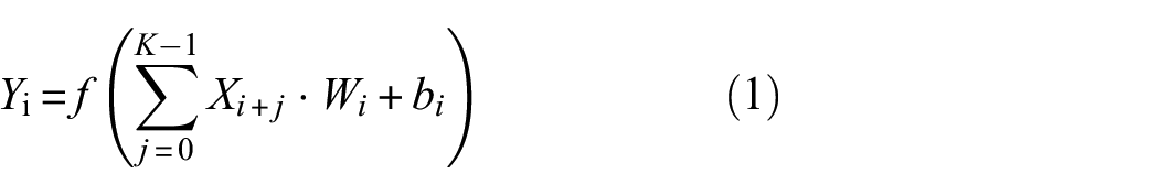
where
Pooling
Pooling operations play a crucial role in reducing the input parameters and computational burden of a model, consequently addressing overfitting while bolstering its generalization capability. 33 Within 1D-CNNs, prevalent pooling techniques include average pooling and max pooling, represented by Equations (2) and (3), respectively,
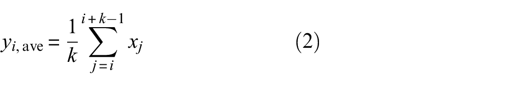
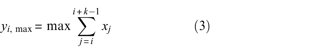
where
Batch normalization
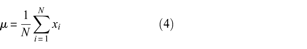
Batch normalization is a common regularization technique whereby normalizing the inputs of a neural network can enhance the model’s training speed.
34
The computed sequence mean and variance are denoted by
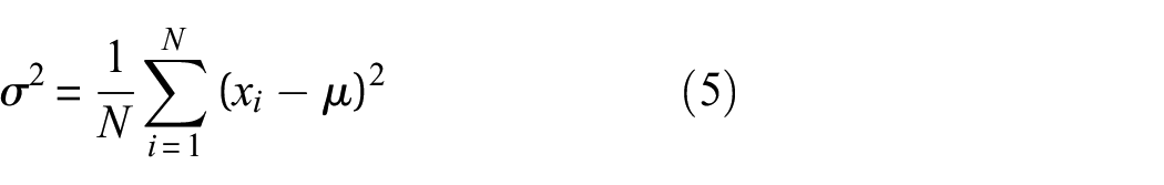
The normalized output is
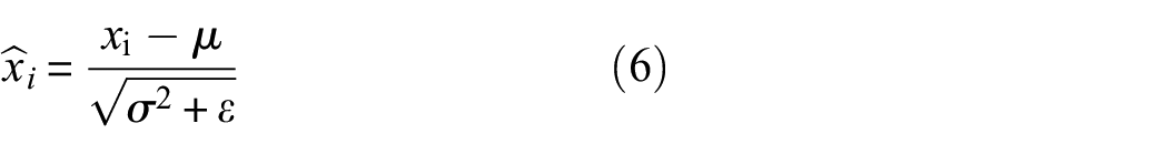
where
After normalizing the data, the linear transformation and bias operations are applied, yielding the normalized output:

where
Activation function
To bolster the model’s nonlinear fitting capacity, it is imperative to employ nonlinear transformations on the data within the neural network’s computational framework.24,35 This is undertaken to optimize fitting outcomes. Among the commonly utilized nonlinear activation functions are sigmoid, tanh, and Rectified Linear Unit (ReLU). However, both the sigmoid and tanh activation functions may confront the challenge of the vanishing gradient phenomenon, particularly when inputs tend toward extremes, leading to gradients nearing zero. ReLU offers a measure of alleviating this issue by maintaining a constant gradient of 1 in the positive domain, thereby circumventing certain instances of gradient disappearance. Notably, ReLU outputs zero for negative inputs, fostering neuron sparsity and bolstering the network model’s resilience and generalizability.
Grad-CAM
The opaque characteristics inherent in neural network models pose a substantial constraint on their applicability, underscoring the importance of elucidating the learning and feature extraction mechanisms within these models. Selvaraju et al. 21 introduced the Grad-CAM method, which employs gradient values obtained through backpropagation as weights, and utilizes heatmaps to depict the neural network’s prioritization of the input data features during the learning phase. In the realm of image classification, Grad-CAM has exhibited notable interpretability, thereby facilitating comprehension of the model’s predictive mechanisms. The principal workflow and underlying principles are delineated as follows:
Upon completion of neural network training, we first compute the gradient of the score
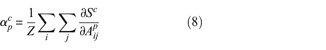
where
The feature maps

The final generated heatmap can be overlaid onto the original input image to visualize the model’s attention across different regions of the input image.
Singular spectrum analysis
SSA is a nonparametric analytical technique applied for processing time series data. Its fundamental approach revolves around converting time series data into a collection of orthogonal basis functions, subsequently subjecting them to decomposition and reconstruction, thus facilitating the decomposition of the original time series. SSA comprises two main stages, decomposition and reconstruction. The decomposition phase encompasses embedding and singular value decomposition (SVD), while the reconstruction phase entails grouping and diagonal averaging. 36
Embedding
Setting the length L of the sampling window, we slide it along the original time series to obtain subsequences

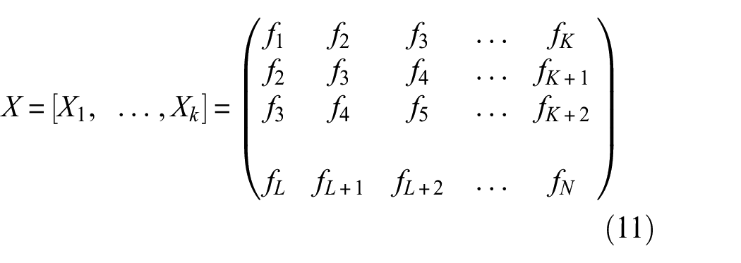
where L is the window length, N is the length of the original time series,
Singular value decomposition
Performing SVD on


where
Grouping
The decomposed singular vectors are clustered based on the information of the singular values and singular vectors, and similar singular vectors are grouped into one group. The matrix is divided into m disjoint subsets, from which Formula (12) can be rewritten as

Diagonal average
For any matrix, its elements are
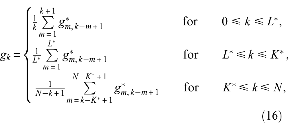
where if
The purpose of diagonal averaging is to transform the matrix
Interpretable health monitoring network model framework
This study uses acceleration signals from a structure under different damage conditions as feature indicators of its structural health. These signals are fed into a one-dimensional CNN for signal classification, and the classification results are used to assess the extent of structural damage. Moreover, by integrating Grad-CAM, the model discerns the level of attention allocated to various segments of the input signals during the learning phase. Through the integration of SSA, an interpretable neural network model for structural health diagnosis is developed. This approach aids in comprehending the internal feature extraction and learning mechanisms of the CNN model. The key features of this interpretable one-dimensional convolutional network model include the following:
One-dimensional time-series data are considered feature data that represent structural operational states for data classification. Therefore, the commonly used two-dimensional CNN is adjusted for one-dimensional input.
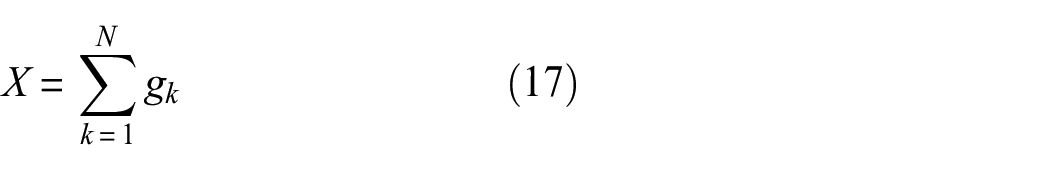
Batch normalization layers are introduced into the model, comprising a calculation unit consisting of convolution, batch normalization, an activation function, and pooling, as depicted in Figure 1, to enhance the computational convergence speed of the model. After completing the calculation of these columns on the input array, each calculation unit passes the output array to the next calculation unit.
Grad-CAM is integrated into the model to compute the gradients of class scores with respect to the convolutional layers, thereby weighting the convolutional feature maps and summing them. These weighted maps are then projected onto the input signal to generate heatmaps that illustrate the model’s activation levels in relation to the input. These heatmaps highlight the focus in the neural network’s learning process.
The SSA method decomposes the input structural vibration acceleration signal into several nonoverlapping modal subsequences, each revealing the signal’s periodicity. When combined with the Grad-CAM activation heatmaps, this approach offers an intuitive visualization of the model’s periodic high-activation learning behavior.
Schematic diagram of individual calculation units in convolutional neural networks.
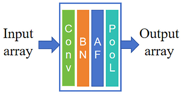
The neural network framework of this article is illustrated in Figure 2. The input is the acceleration time history data sampled by sliding, and the output is the classification label used to determine the structural state.
Interpretable health monitoring network model framework.
Experimental process and data preparation
A scaled-down single-layer frame structure is fabricated in the laboratory to conduct small hammer impact tests. Acceleration time-series data from beam components under diverse joint damage conditions are then gathered using acceleration sensors. These data accurately depict the operational states of the structure across varying degrees of joint damage. Subsequently, the collected data are utilized as training inputs for the previously introduced neural network model.
Test process
To obtain the acceleration data of the prefabricated structures at different damage states at the joints, a reduced-scale single-story prefabricated steel frame is constructed by connecting beam-column members using high-strength bolts and L-shaped connectors. Dynamic tests are then conducted based on this setup to measure the acceleration data of the beam members under various damage conditions. The steel beams are connected to H-shaped steel columns at both ends using six high-strength bolts and two L-shaped connectors, as illustrated in Figure 3. The beam used in the experiment had a length of 1.45 m and a rectangular section measuring 0.08 × 0.008 m. The beam was connected to the columns, which had a height of 0.5 m and a universal column section measuring 0.1 × 0.08 × 0.008 m. This connection was achieved using four gusset angles with a section size of 0.05 × 0.05 × 0.004 m. To ensure a fully tightened condition, a pretension torque of 60 Nm was applied to the 12 high-strength bolts with a diameter of 10 mm using a torque wrench. For stability, the columns were affixed to the laboratory floor using long bolts to provide fixed supports at the bottom, as depicted in Figure 4.
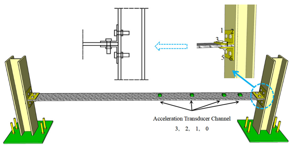
Schematic diagram of experimental layout.
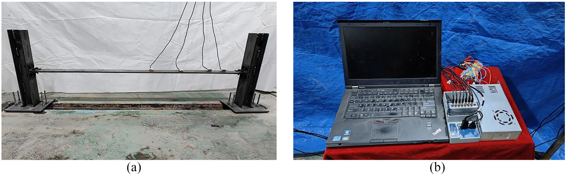
Experiment schematic of steel frame dynamic tests. (a) Reduced-scale single-story prefabricated steel frame and (b) signal acquisition system.
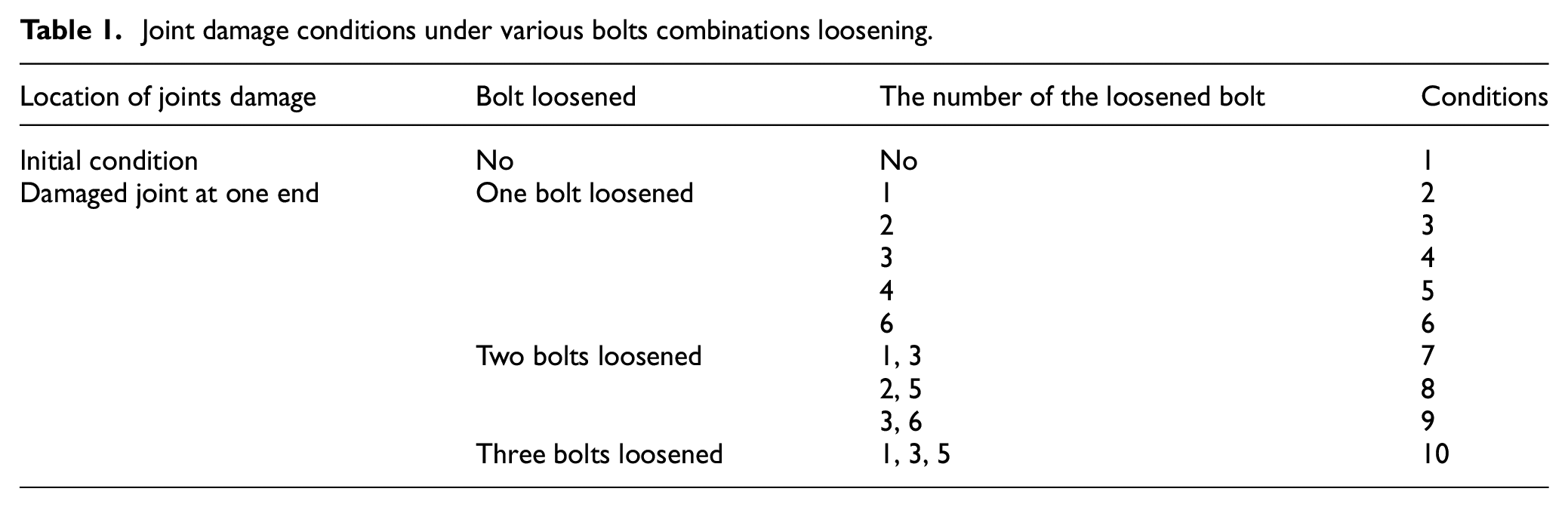
In theory, it is essential to replicate a diverse range of damage scenarios since structural damage occurrences in real-world situations are stochastic, leading to an extensive spectrum of potential damage conditions. Consequently, it is crucial to identify a representative subset of these scenarios to evaluate their acceleration signals accurately. To simulate the damage at the joint, we induced damage by loosening the high-strength bolts and fully releasing their preload tension. This study examines 10 conditions, comprising one healthy condition and nine damaged conditions, delineated in Table 1. The healthy condition (Condition 1) serves as the baseline for all the damaged conditions, while Conditions 2–10 encompass various combinations of potential loosening scenarios for single-side bolts. In this study, the structure state is limited to these 10 damage conditions.
Joint damage conditions under various bolts combinations loosening.
During accelerometer placement, the 0.05 m ends attached to the connectors are treated as part of the joint, forming an integrated connection area. The calculated length of the beam is fixed at 1.35 m. Four accelerometers are strategically positioned along the beam’s length at intervals of 0.1, 0.2, 0.4, and 0.6 m from the structure, as depicted in Figure 5. Structural vibrations are induced by impacting the structure with a hammer, targeting the impact point at 0.5 m along the beam to avoid the nodal positions of the structure’s initial vibration modes.
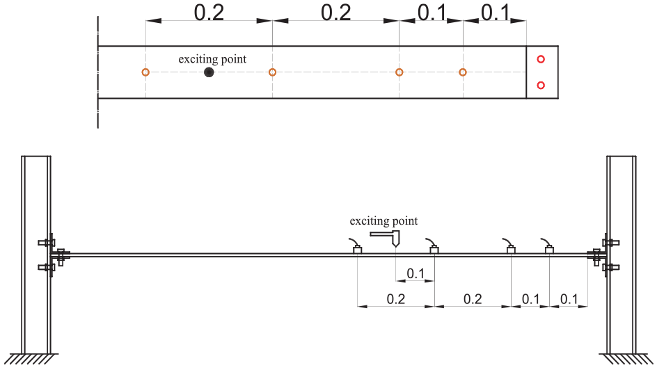
Layout of accelerometer.
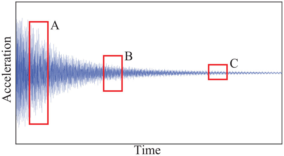
Throughout the experiment, the sampling frequency of the data acquisition instrument was set at 1000 Hz to capture the acceleration time history curves at each measurement point, as depicted in Figure 6. A typical acceleration time history curve is delineated into three segments (A, B, C). Segment A denotes the transition from the structural equilibrium state to impact acceptance. During impact, the interaction between the impact hammer and the structure is fleeting, influencing the data collected during this phase. Segment C reveals that the structure’s vibration decreases to a narrower amplitude range. Environmental noise can notably perturb the data during this interval. Consequently, we opt for an acceleration time history curve depicting the stable decay of the structure for data processing. Specifically, data from segment B are selected for segmentation and enhancement as inputs for training the neural network model, as illustrated in the figure.
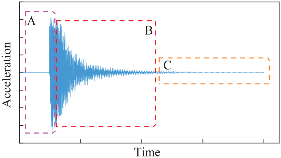
Typical acceleration time history curve.
Noise
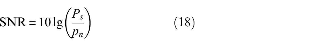
To evaluate the robustness of the network model, the experimentally obtained data were subjected to noise augmentation. If the model sustains a satisfactory level of accuracy when handling temporal data across different noise levels, this suggests the model’s robustness. The noise magnitude is determined by the power of the original signal and the signal-to-noise ratio (SNR). Modulating the signal-to-noise ratio allows for regulating the noise’s influence on the data. The calculation formula for the SNR is provided below:
In this study, Gaussian noise with SNRs of 50, 10, and 5 dB is used, as illustrated in Figure 7.
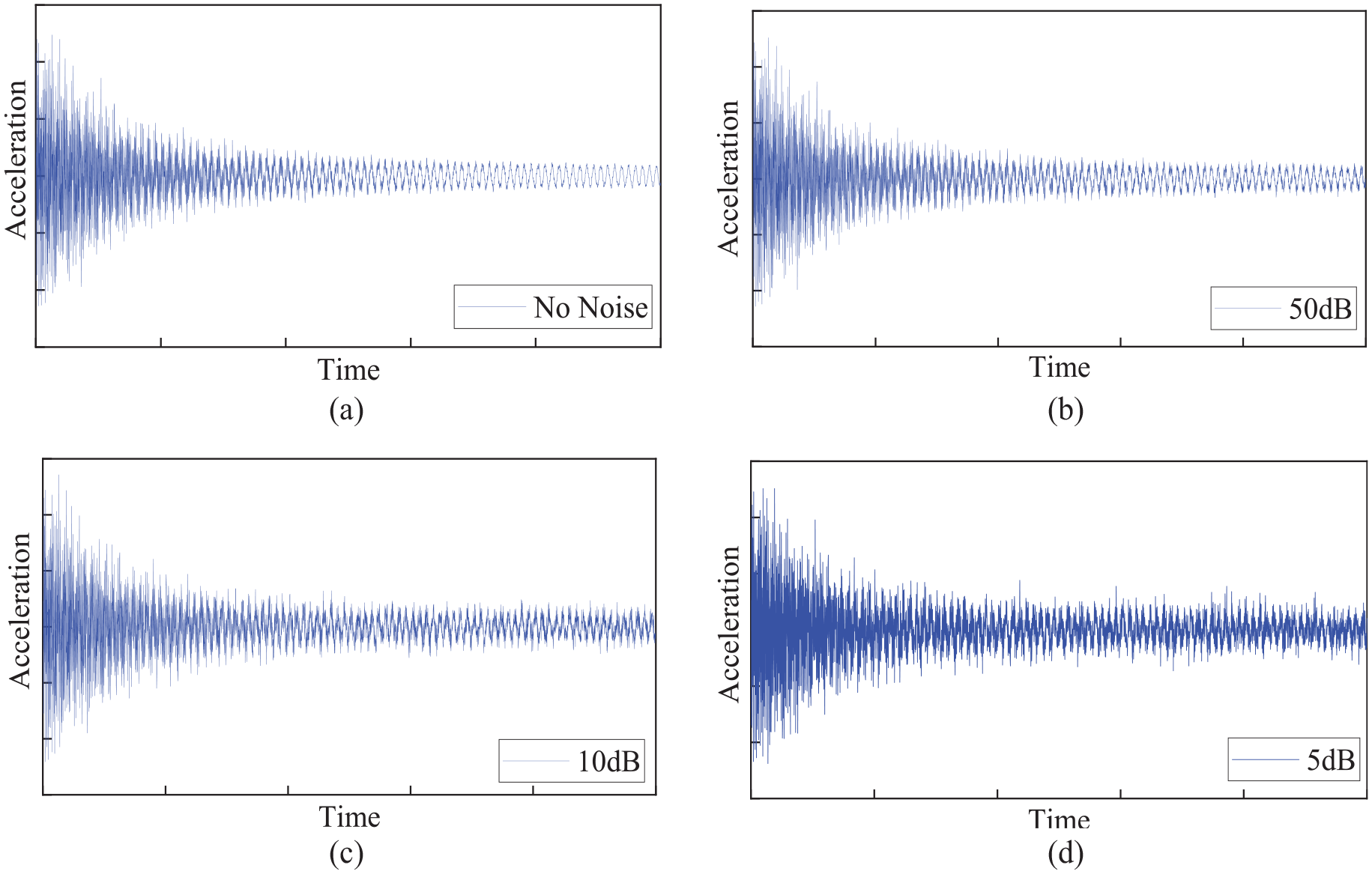
Experimental data with various levels of noise. (a) No noise, (b) 50 dB, (c) 10 dB, and (d) 5 dB.
Data augmentation
Employing acceleration time-series curves to train deep learning models under different structural damage conditions requires a substantial amount of data to ensure the stability of the network model. Therefore, data augmentation becomes imperative. Considering practical constraints, the data are segmented with an overlap, extracting S acceleration data points per slice, and then shifting by W acceleration data points, resulting in n data samples, as illustrated in Figure 8.
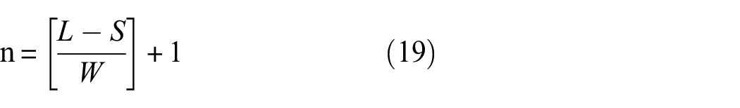
where L represents the total length of the signal; S represents the sample length; W represents the data offset; and [ ] is a rounding operation.
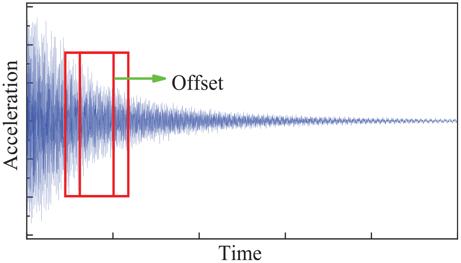
Data augmentation based on sliding sampling:
Utilizing the described data augmentation technique, a sliding sampling approach was employed on the 5000 experimental data points, utilizing a sliding window of 2 data points for each sampling instance. Four distinct sampling lengths were employed: 500, 200, 100, and 50. Across each experimental condition, these four sampling strategies yielded sample sizes of 2251, 2401, 2451, and 2476, respectively. Across the entirety of the 10 experimental conditions, 22,510, 24,010, 24,510, and 24,760 cumulative data samples were obtained. This methodology serves to augment the sample library for signal classification, ensuring a substantial volume of data for model training, thereby facilitating the development of a more robust model.
Hyperparameter settings
The training configuration for the neural network was set using the Adam optimizer with the following parameters: the training was conducted on a multi-GPU environment to accelerate computation. The network was trained for a maximum of 1000 epochs, with an initial learning rate of 0.001. L2 regularization was applied with a coefficient of 1e-4 to prevent overfitting. The learning rate schedule was set to piecewise, where the learning rate decreases by a factor of 0.1 after every 500 epochs. The training data were shuffled at the beginning of each epoch to ensure the model generalizes better. During the model training process, we divided the dataset into an 80% training set and a 20% testing set.
Results and discussion
This section discusses and analyses some parameters that may affect the training accuracy of the model, including the depth of the model, sensor position, input data length, and noise. In this section, we will use the accuracy of the test set to characterize the accuracy of the model.
Model depth
The calculation unit proposed earlier undergoes convolution, normalization, activation, and pooling sequentially to extract features from the data. Increasing the depth of the network according to the data characteristics gradually enhances the model’s capability for data processing and feature extraction. However, beyond a certain threshold, increasing the network depth may lead to a decrease in model training accuracy, potentially resulting in overfitting. Therefore, investigating the appropriate depth of the model is essential for achieving high accuracy while maintaining training efficiency. Taking data samples with a length of 200 as an example input for the model, the number of calculation units is gradually increased from 2 to 7. The impacts of the number of calculation units on the model accuracy and training time are compared. According to the training results, when the number of calculation units reaches 4, the model’s accuracy exceeds 97%. However, increasing the number of units beyond seven leads to a decrease in training accuracy, and the training time of the neural network model gradually increases with an increase in the number of calculation units, as shown in Figure 9. In summary, in practical applications, it is crucial to select an appropriate depth for the network model based on the characteristics of the dataset to ensure both training accuracy and efficiency. In the model presented in this article, setting the number of calculation units to 4 ensures that training accuracy is maintained while also reducing the training time.
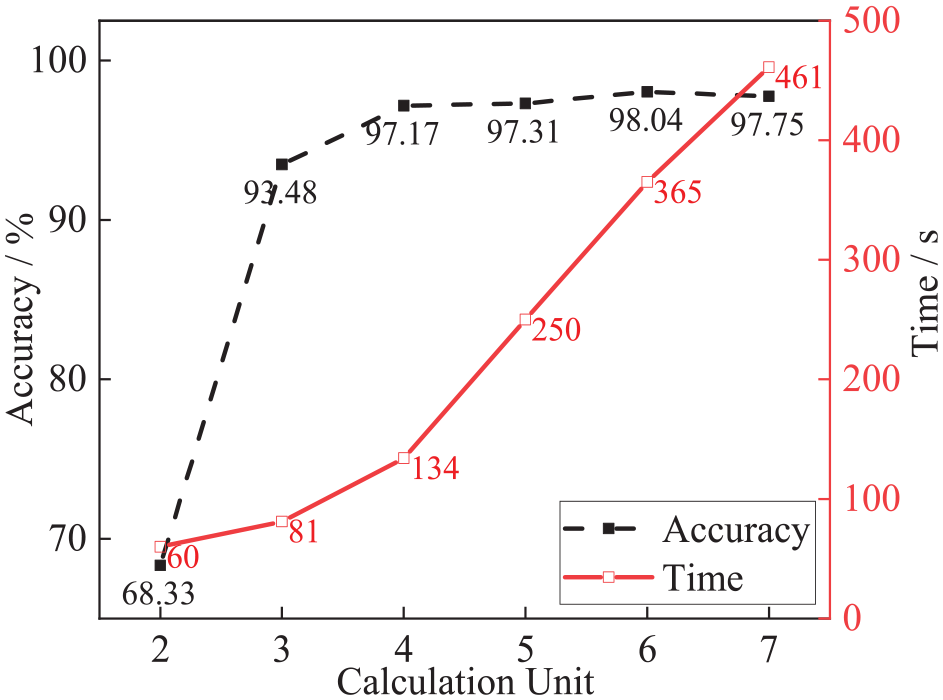
The impact of the number of calculation units on network accuracy and training time.
Location of sensors
Throughout the experimental procedure, four accelerometer sensors were positioned along the beam’s length. Subsequent to each impact, acceleration time-series data were collected from all four channels. Owing to variations in the sensor placement, each sensor captured location-specific acceleration time-series data under various conditions. Our aim is to ascertain whether the acceleration data from each position can be used to train a neural network to attain the predetermined accuracy and establish a robust discriminative model. Following the data augmentation across all four sensors, the sensors were trained using identical neural network architectures to compare the training accuracies corresponding to different positions. The model training outcomes reveal that data from all four channels significantly contribute to damage classification, achieving training accuracies surpassing 97%, as illustrated in Figure 10. In this experiment, the data recognition accuracy for Channel 2 is the highest.
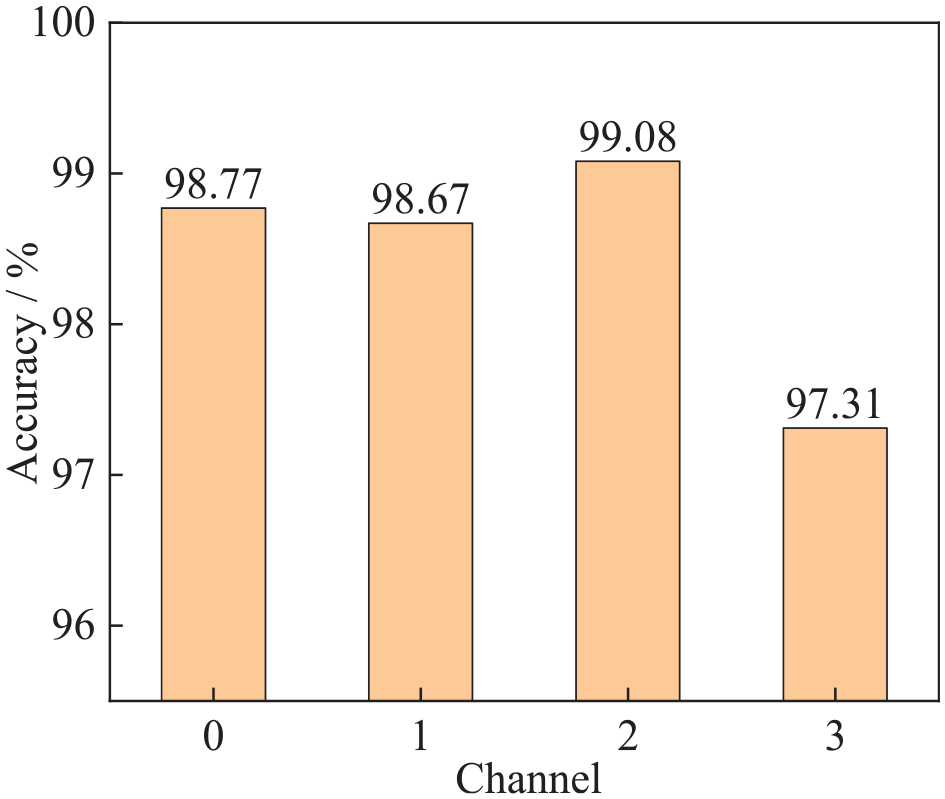
Comparison of training accuracy for sensor data at different channels.
Data length
To ensure the accuracy of the neural network, it is advisable to select shorter data segments as inputs for the model. Shorter data segments can reduce the number of learning parameters during the training process. Additionally, under a constant sampling frequency, utilizing shorter data segments for training indicates that the model can assess inputs within a shorter timeframe, thereby ensuring timely responsiveness. As shown in Figure 11, as the length of the input data decreased from 500 to 50, the training accuracy of the model decreased from 98.93% to 89.12%. It is evident that as the length of the input data to the neural network decreases, the model’s accuracy tends to decrease. Therefore, when determining the length of the input data, it is essential to choose data segments that are as short as possible while ensuring sufficient model accuracy, thus enhancing the computational efficiency of the model. In this experiment, when the data length exceeds 100, the model achieves a recognition accuracy greater than 96%. This indicates that, under practical conditions, data samples with a duration of 0.1 s or longer can be accurately classified.
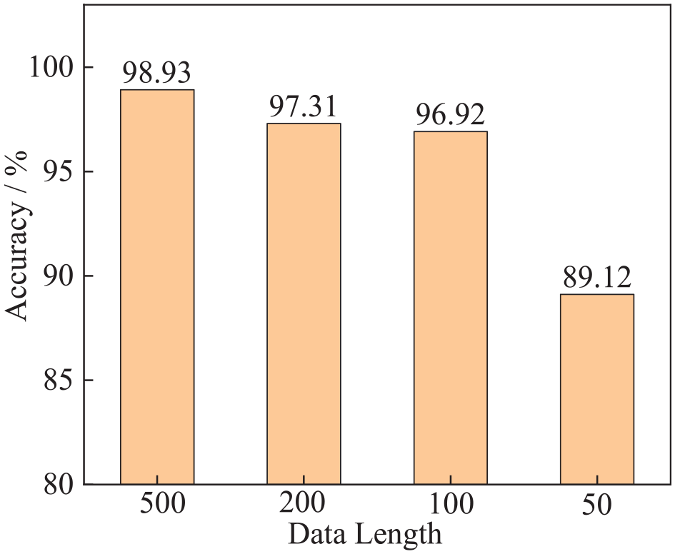
The effect of data length on model training accuracy.
Impact of noise
The data obtained in the experimental environment already include some white noise and operational precision effects inherent to laboratory settings. However, the controlled nature of the laboratory environment diminishes the numerous sources of noise compared to real-world conditions, yielding relatively cleaner data. Channel 3 data were selected, and noise levels of 50, 10, and 5 dB were applied to assess the accuracy of the neural network model and validate its robustness. Our analysis of the training results reveals the model’s ability to accurately discern signals amidst varying degrees of noise across different damage conditions. Remarkably, the model consistently achieved an accuracy exceeding 97%, as shown in Figure 12, underscoring its exceptional robustness.
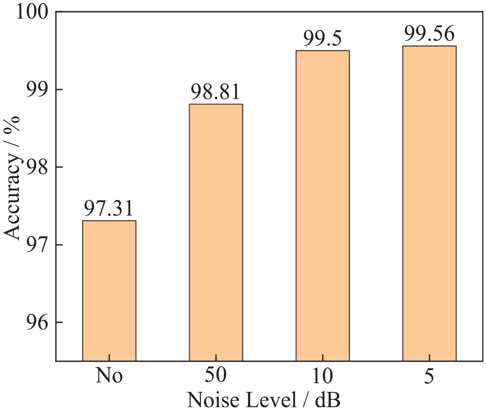
Training accuracy of models under different noise levels.
Interpretability of the health monitoring network model
Signal SSA
During the process of structural vibration attenuation, vibrations characterized by different frequencies exhibit diverse decay rates. Typically, higher-frequency vibration modes undergo more rapid decay than lower-frequency modes, owing to the swift dissipation of the energy inherent in high-frequency modes. As a result, the participation of vibration modes across different frequencies fluctuates over time, posing challenges in identifying temporal patterns from the original signal at various time scales. To address this issue, Channel 3 data serve as an illustrative example, where we employ SSA. Through parameter adjustments within SSA, we isolate the subsequences corresponding to the initial six modes, labeled SA1–SA6, whose temporal and spectral characteristics are detailed in Table 2. A comparison between the frequency values derived from the Fourier transform (FT) of the original signal, and those obtained through SSA, indicates negligible disparities, as illustrated in Figure 13 and Table 3. This alignment underscores the effective extraction and segregation of the initial six modal acceleration signals in the time domain using SSA.
Time and frequency domain analysis of subsequences obtained from SSA of original signals.
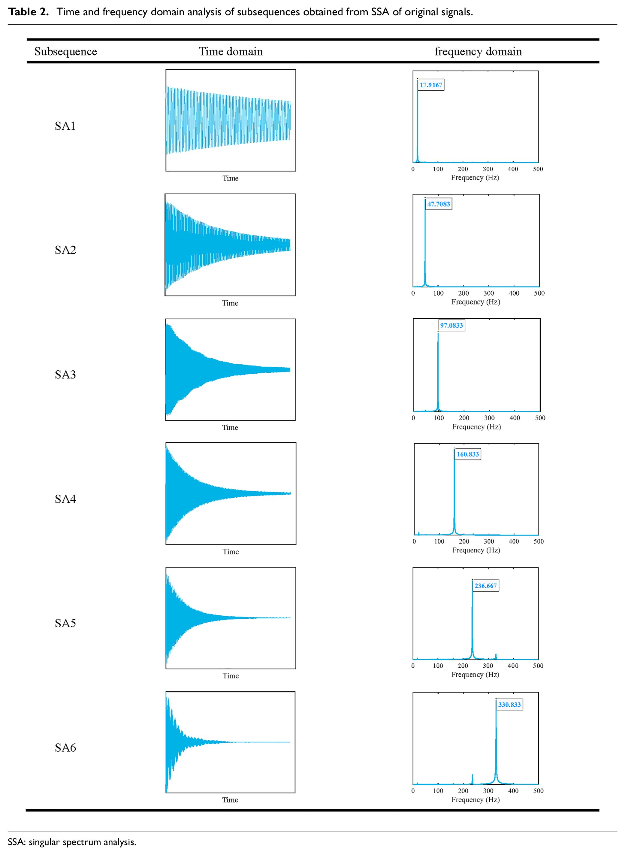
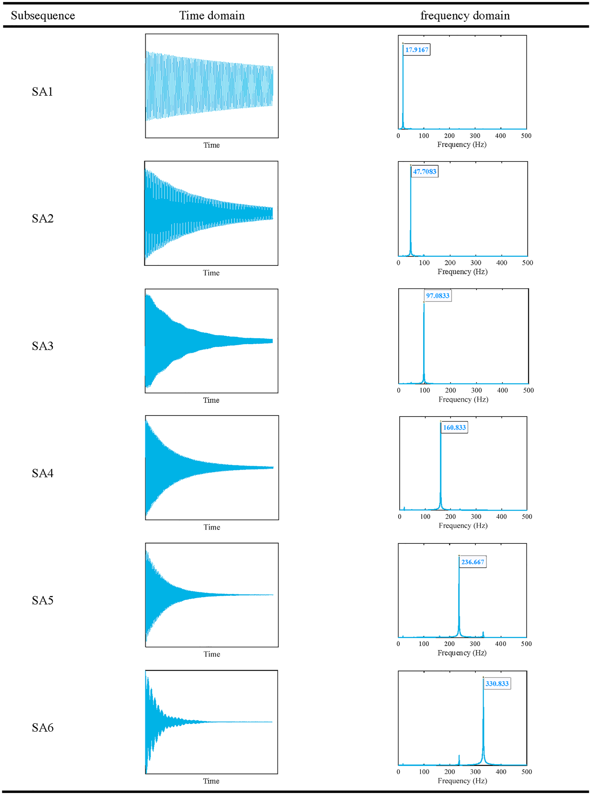
SSA: singular spectrum analysis.
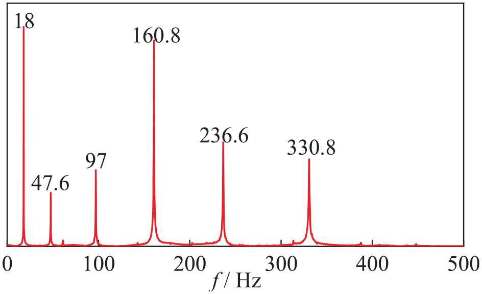
Frequency domain obtained by Fourier transform of the original signal.
Comparison of various frequency values for Fourier transform and SSA.
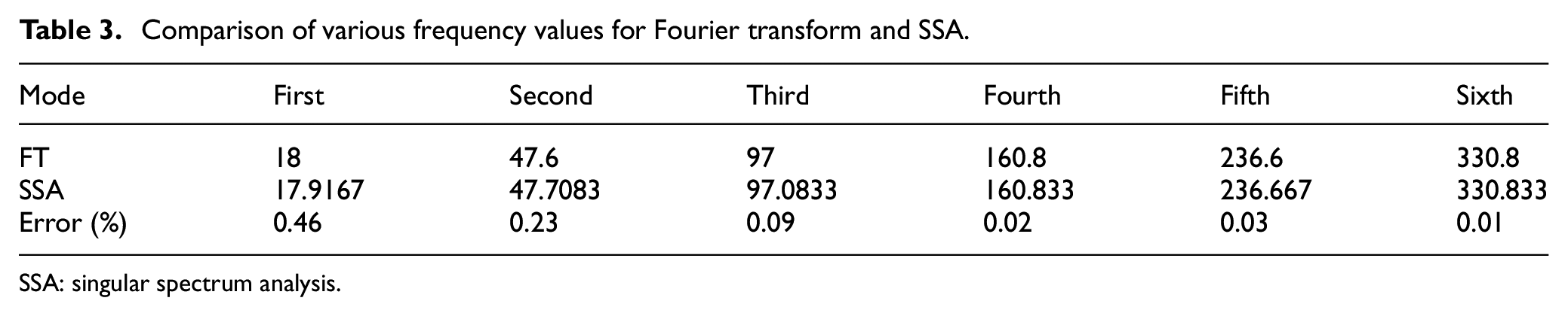
SSA: singular spectrum analysis.
Visualization of network model learning
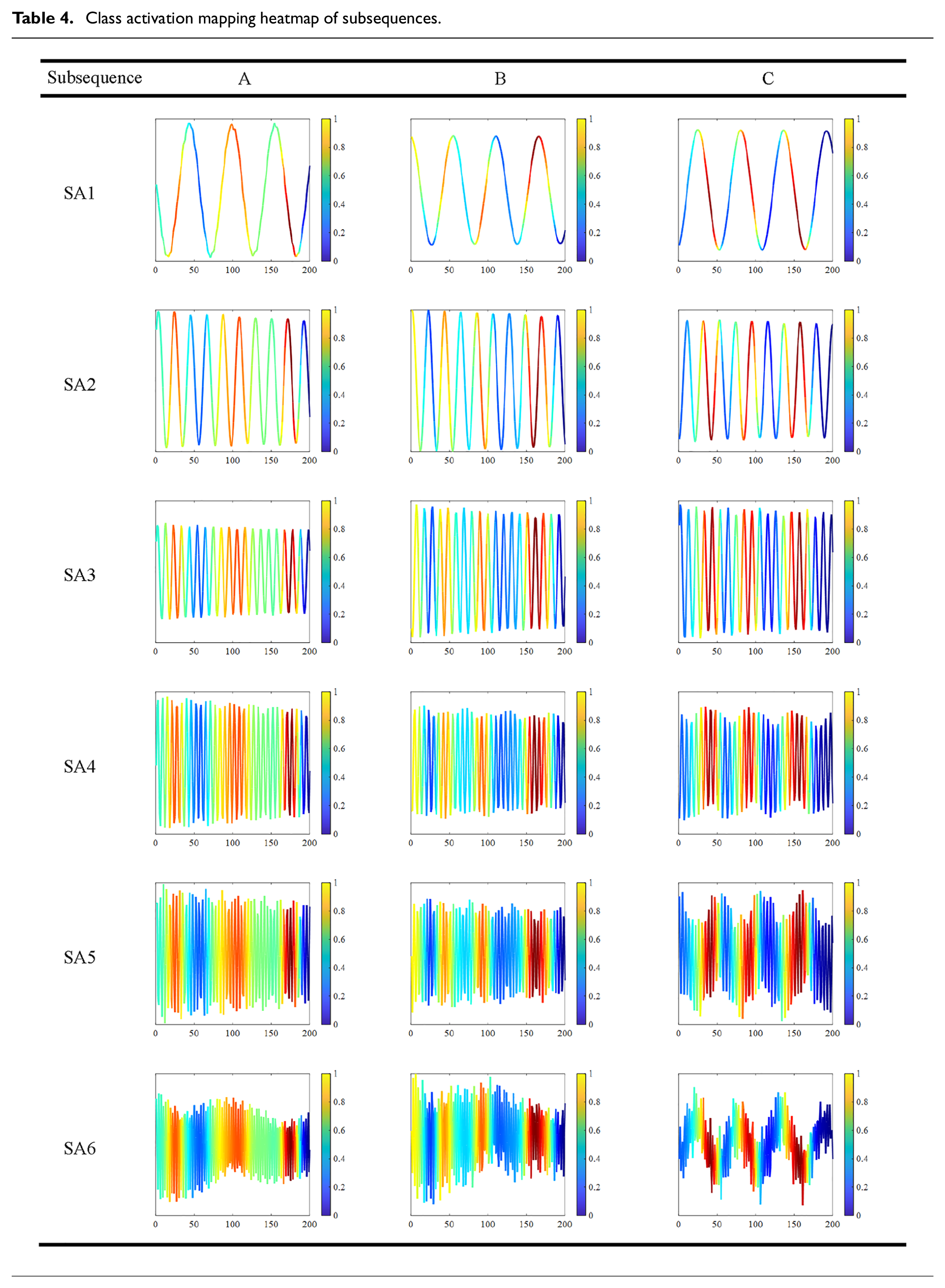
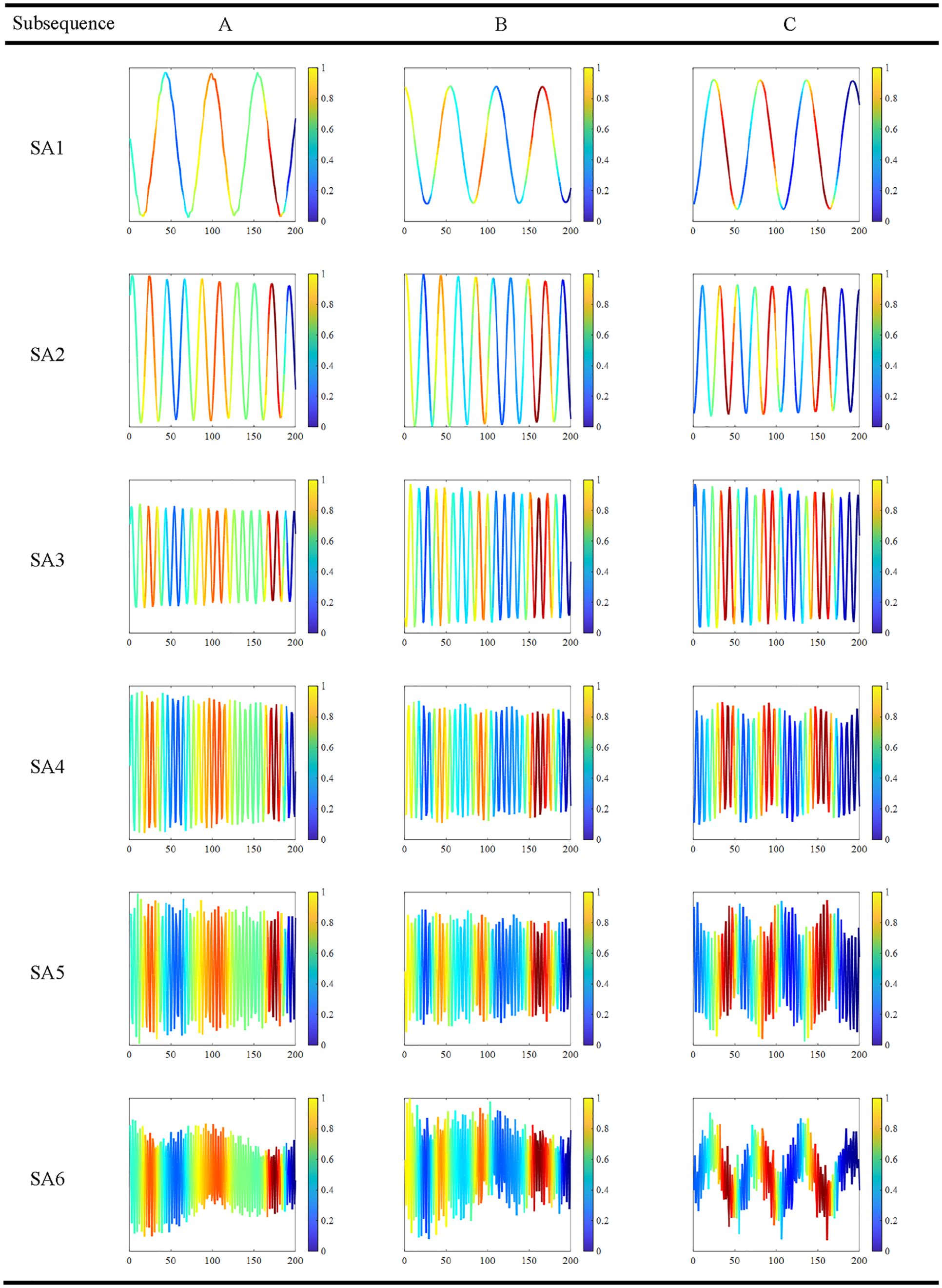
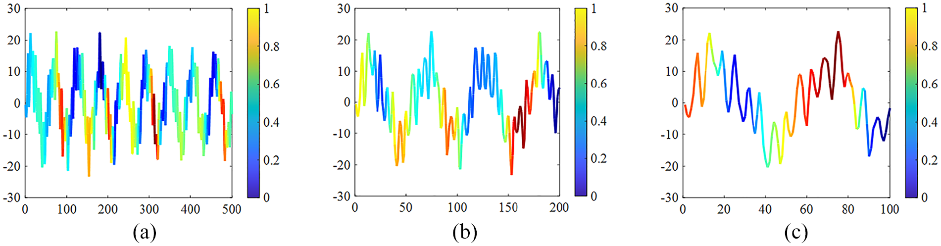
Structural vibration, a process of free decay, exhibits the characteristics of nonstationary signals to a certain degree. Therefore, three signals (A, B, C) are extracted along the time axis for an analysis of their activation levels, as illustrated in Figure 14. These signals are then input into the trained model, and the Grad-CAM method is employed to compute the gradient weights of each signal. Through class activation mapping, heatmaps are generated to depict the significance of various segments within the input signals during the feature extraction process, with the darker hues indicating greater attention during learning. The resulting activation maps are depicted in Figure 15. The contribution of a neural network model in the process of signal classification decision-making can be reflected by the values of CAM, with higher values indicating greater contribution during the decision process, and lower values suggesting less contribution. Through the visualization provided by Grad-CAM, it is possible to reveal which specific local feature regions the neural network relies on when making classification decisions, thus providing an intuitive basis for understanding the model’s decision-making process. As seen in Figure 15, the signal is periodically highly activated, indicating that the decision-making process depends on the periodic features of the signal. This method helps researchers better understand the model’s working mechanism, assess its reliability, and even uncover potential biases or errors. Additionally, mapping Grad-CAM values to their corresponding decomposed subsequences produces the subsequent graphs detailed in Table 4. Based on SSA, subsequences corresponding to each modal component of the signal were obtained, with each subsequence exhibiting distinct periodic characteristics. Furthermore, periodic high-activation phenomena were observed during the signal learning process in the heatmap. This suggests that the neural network model has successfully identified the inherent periodic features within the signal. This presence of periodic activation signals enables signal classification, thus achieving the classification of signals during the learning process.
Signal interception.
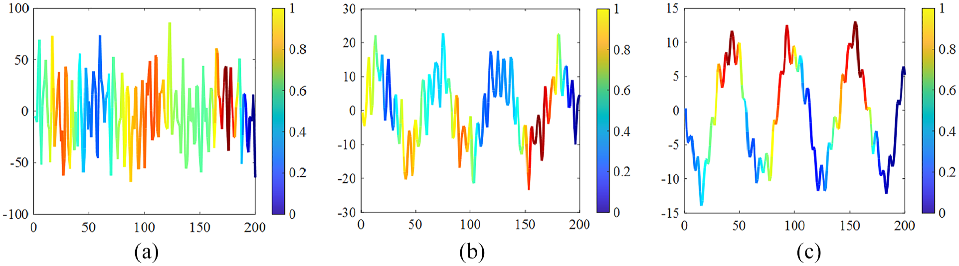
Heatmap of class activation mapping for input signals. (a) Signal at location A, (b) signal at location B, and (c) signal at location C.
Class activation mapping heatmap of subsequences.
Explanation of the influence of parameters
Data of different lengths
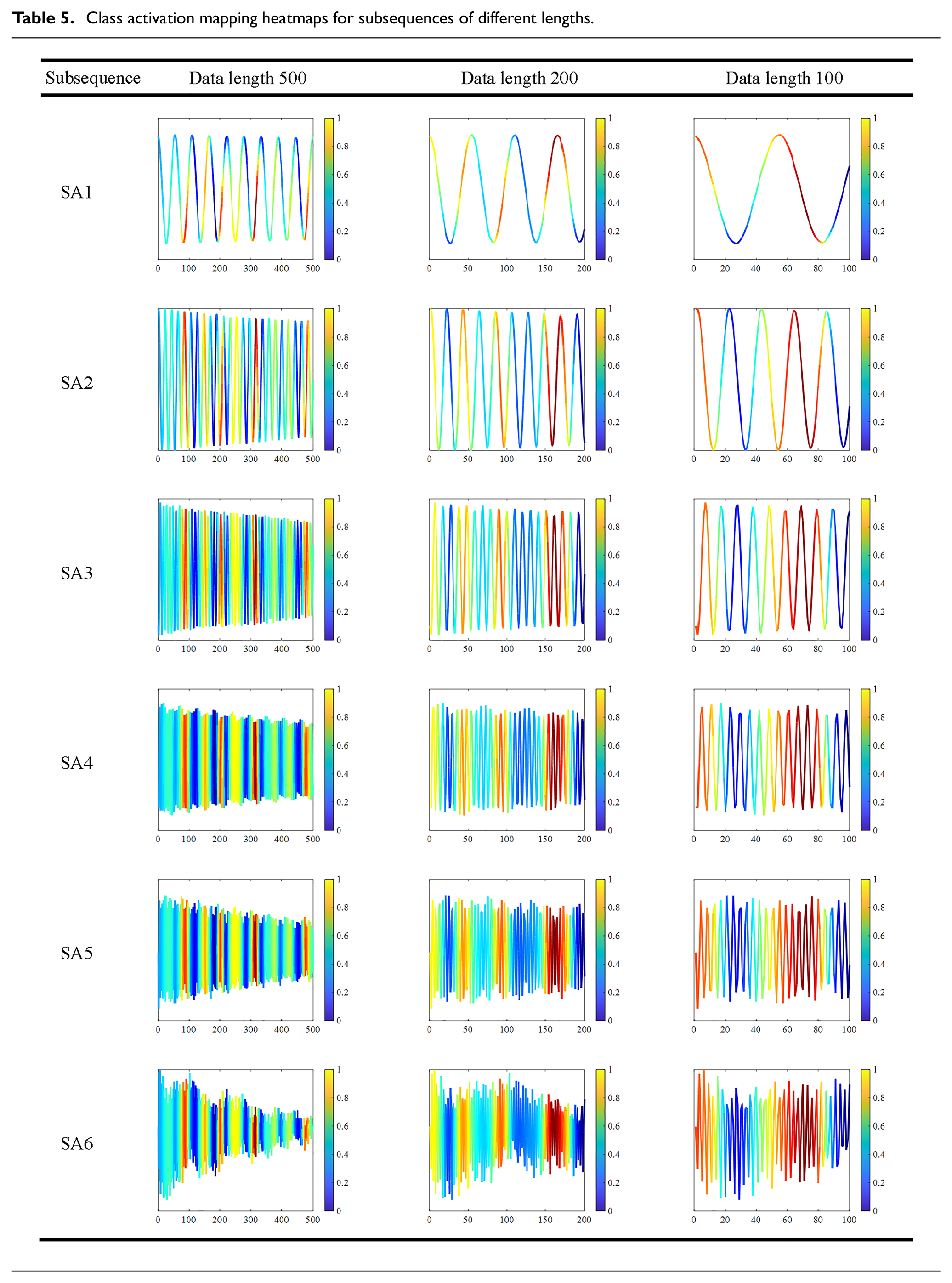
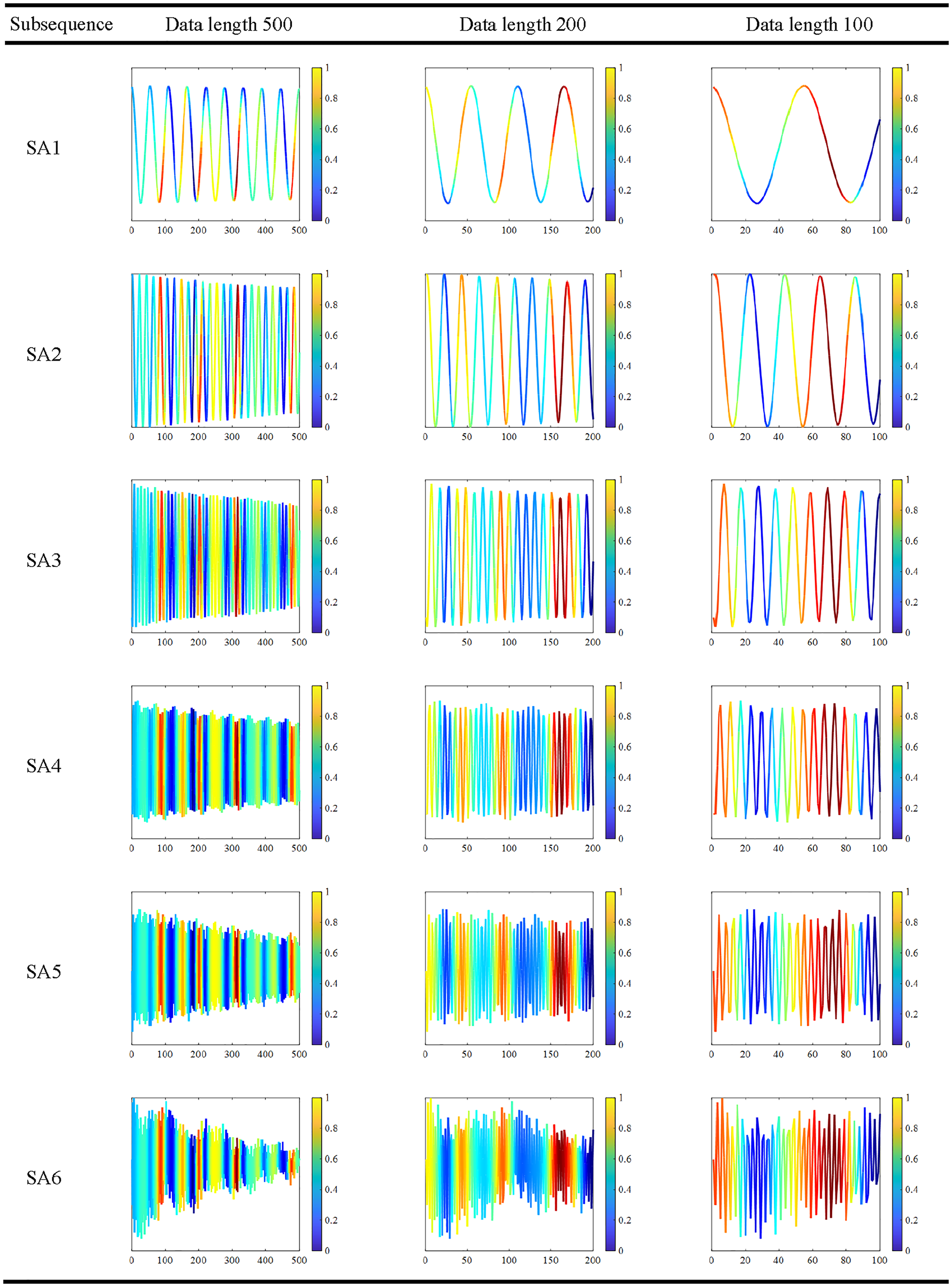
In the previous analysis of parameter influence, it was observed that training the network with data of different lengths impacts its accuracy. Particularly, when the data are excessively short, the model’s precision significantly decreases. This phenomenon is elucidated by comparing the class activation mapping graphs corresponding to the various data lengths, depicted in Figure 16, along with the corresponding subsequent class activation mapping heatmaps presented in Table 5. The periodic activation signal phenomenon persists across varying data lengths. Notably, as the data length decreases gradually, the number of signal cycles that the network can learn also decreases. This reduction in signal cycles progressively complicates network regression, resulting in an incremental increase in the complexity of network learning and a corresponding decrease in training accuracy.
Class activation mapping heatmap for input data of different lengths. (a) Data length 500, (b) data length 200, and(c) data length 100.
Class activation mapping heatmaps for subsequences of different lengths.
Data from different channels
Acceleration signals can be received at different sensor positions. To optimize the experimental setup, considering the characteristics of the first six-order modal shapes, the sensor layout was designed to minimize proximity to the nodes of these modes, as illustrated in Figure 17. In Figure 17, we can observe that the level of participation of each sensor in different modal frequencies varies depending on its position. This results in different acceleration information being received by each sensor, leading to discrepancies in the recognition accuracy of the data across different channels. The participation level of each modal shape order varies across sensor positions, resulting in distinct spatial attributes for signals received at different locations. The Fourier transformation of the acceleration time history signals from each sensor produces frequency domain signals, as depicted in Figure 18. The magnitude of each frequency domain peak reflects the involvement of the respective order signals at different sensor positions. Although the signals received by sensors at each position have their own spatial attributes, they are sufficient to accurately assess structural health information, demonstrating the excellent generalization performance of the network model.
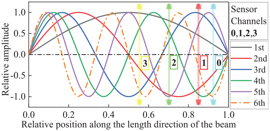
The position of the sensor relative to the first six vibration modes.
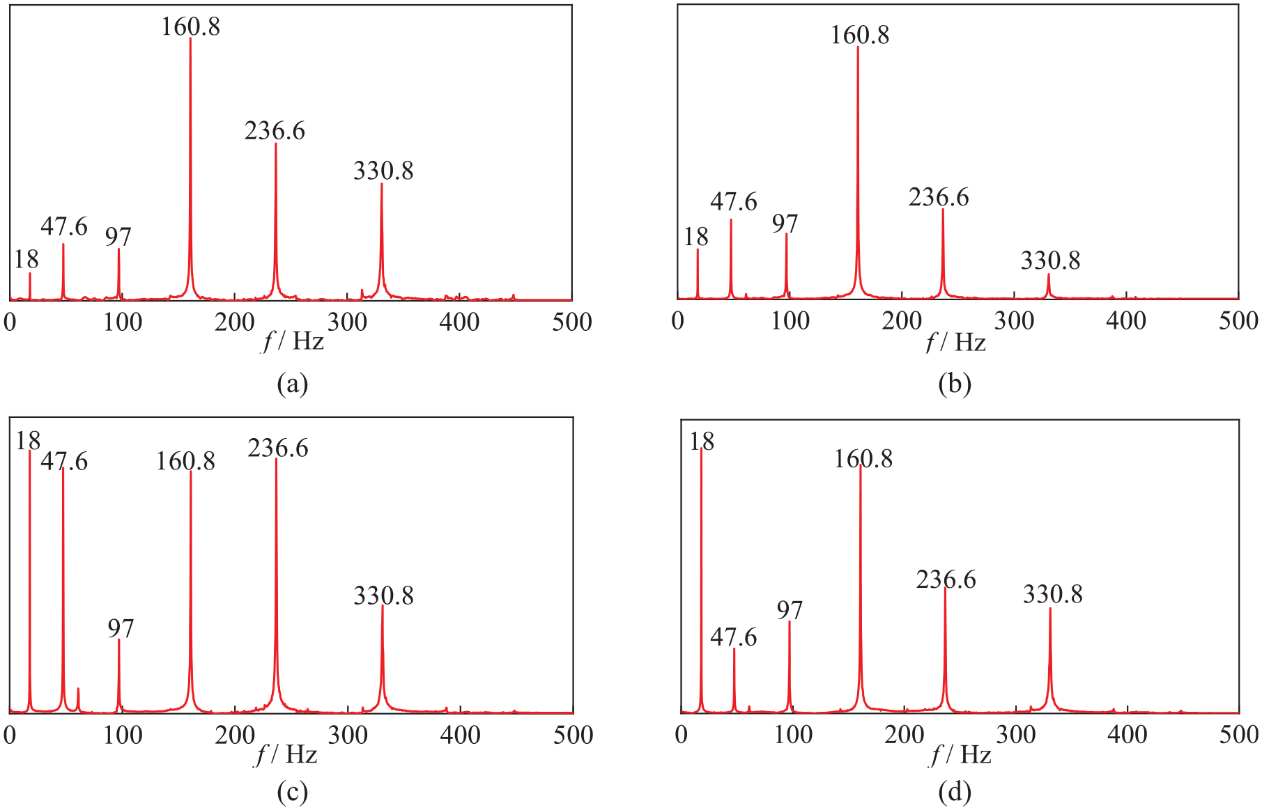
Frequency domain data obtained from Fourier transform of each channel under initial conditions. (a) Channel 0, (b) Channel 1, (c) Channel 2, and (d) Channel 3.
Data with added noise
The model proposed in this article still demonstrates high recognition accuracy for noise data at various levels, indicating its robustness. Fourier transformation of the noisy data reveals that the frequencies of different orders remain largely unchanged, as depicted in Figure 19. Therefore, the model’s periodic activation learning can still extract features effectively, enabling accurate judgments even in the presence of noise. Furthermore, the application of noise increased the diversity of the data, reducing the risk of overfitting and leading to an improvement in the model’s recognition accuracy, as demonstrated in section “Impact of noise” of this article.
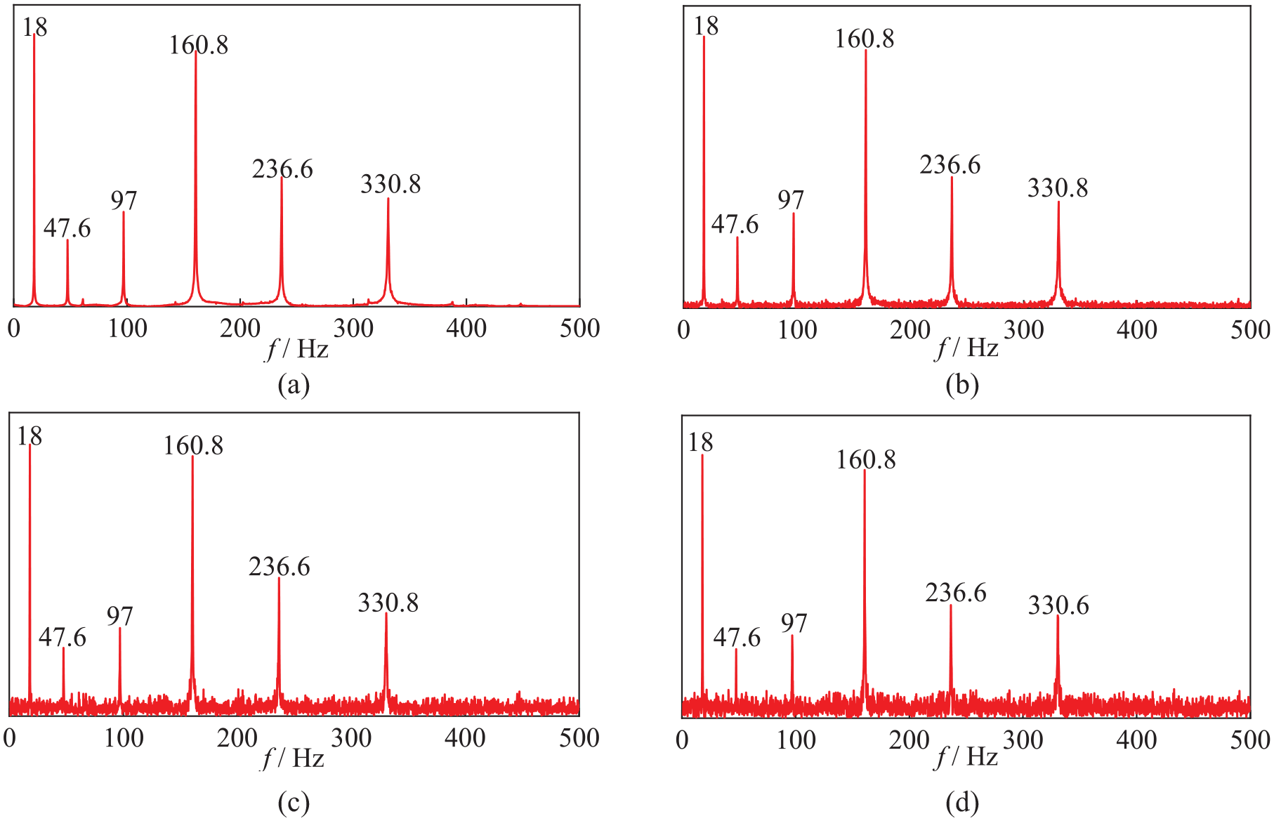
The first six frequency domains obtained by Fourier transform of signals at various noise levels. (a) No noise, (b) 50 dB, (c) 10 dB, and (d) 5 dB.
Comparison between neural network models and traditional spectral analysis methods
Traditional spectral analysis methods
The methodology for diagnosing structural damage through spectral analysis has consistently remained the predominant approach in health monitoring. With advancements in modern signal processing techniques, a myriad of methodologies have been employed in SHM, encompassing Fourier transforms, wavelet transforms, Hilbert–Huang transforms, and others. The utilization of these signal processing techniques furnishes us with further insights into signals across various dimensions encompassing both time and frequency domains. Principally, this diagnostic approach offers exceptional physical interpretability. Additionally, spectral analysis has emerged as a relatively straightforward and intuitive method, necessitating minimal training data and computational complexity. This method expedites the swift extraction of structural frequency information from limited data samples and is thus suitable for preliminary damage detection and diagnosis.
However, spectral analysis methods inherently have limitations. Initially, traditional spectral analysis methods may hinge on specific assumptions, such as signal stationarity and linearity, which may not be applicable to complex signal scenarios. For instance, spectral analysis frequently presupposes linearity in systems, potentially constraining the efficacy of damage diagnoses for nonlinear structures. Furthermore, fluctuations in peak values and frequency components within the spectrogram may be influenced by various factors, thereby mandating the amalgamation of domain expertise and experience.
Neural network models
Utilizing neural network models for signal discrimination offers significant advantages. First, neural networks possess robust nonlinear modeling capabilities, rendering them highly adaptable to complex structural damage issues. This adaptability enables neural network models to effectively detect and analyze subtle damage signals, thereby providing highly accurate diagnostic results. Second, neural network models can undergo end-to-end learning, directly acquiring feature representations and associations from raw input data. This eliminates the need for manual extraction of spectral features, streamlining the diagnostic process and enhancing automation. Moreover, neural network models can be trained on extensive datasets and demonstrate strong generalizability. Once trained, these models can be applied to unknown structures and damage scenarios, facilitating reasonable predictions for new test data.
However, relying on neural network models for structural damage assessments has inherent drawbacks. First, neural network models necessitate abundant labeled data for training to achieve an optimal performance. Consequently, inadequate training data, or poor data quality, may limit the model’s effectiveness in practical applications. Second, neural network models are often regarded as black-box models that lack interpretability. As a result, they cannot directly elucidate the specific localization or causes of the structural damage, and can only provide diagnostic results. Additionally, deep neural networks typically demand substantial computational resources for training, including GPU acceleration and extensive memory.
Comparison of two methods
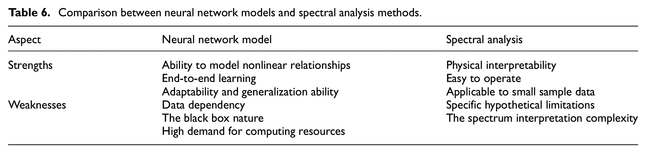
A comparison between traditional spectral analysis and neural network approaches for analyzing and diagnosing structural damage signals reveals their respective strengths and weaknesses, as outlined in Table 6. Traditional spectral analysis excels in its physical interpretability, while neural network models exhibit robust adaptability and generalization capabilities. These complementary attributes prompt the proposal of a method that amalgamates SSA with CNN modeling. This approach leverages the superior computational ability of the neural network models while integrating SSA for visual interpretation and elucidation of the learning process. Consequently, it offers a novel perspective for SHM within the evolving realm of computer technology.
Comparison between neural network models and spectral analysis methods.
Moreover, neural network methods possess the ability to make judgments based on very brief signal durations, a capability beyond the reach of a traditional spectral analysis, which lacks the resolution to differentiate signal variations among different types of damage and provide precise evaluations. In the trained neural network model, extremely short signals can be utilized to monitor structural health, thereby enabling real-time responsiveness in SHM.
Conclusion
This study introduces an interpretable CNN designed for classifying data from 10 distinct damage conditions of a single-layer framework structure. The model achieves satisfactory classification results and demonstrates robustness under various levels of noise. By employing class activation mapping, the network’s attention to input data during the learning process is visualized, providing insight into the focus of the learning. By employing SSA, the input signal is disassembled into a combination of periodic signals, with class activation mapping depicted within these periodic signals, which aid in the comprehension of the network’s learning process. The primary conclusions are outlined as follows:
Through convolutional neural network classification of structural signals, the classification accuracy reaches over 95%, indicating the favorable efficacy of CNNs in addressing such one-dimensional signal classification problems. Such problems are amenable to processing with 1D-CNNs.
The method based on class activation mapping reflects the attention level of the inputs during the learning process, visualizing the phenomenon of periodic highly activated states during learning, which helps us understand the learning process of neural networks and enhances our trust in them.
By comparing the advantages and disadvantages of neural networks and traditional spectral analysis in handling such problems, it was observed that combining the two methods can leverage their respective strengths, achieving real-time responsiveness in structural damage identification.
Overall, our current research faces several limitations: (1) the preset damage of bolts is complete loosening, and the preload is completely released; (2) the experimental environment is relatively simple and does not consider the vibration excitation problem in actual engineering; (3) the performance of the classification neural network may be limited by the choice of training dataset used for signal damage classification; (4) the interpretation of the learning process in CNNs is still relatively underdeveloped.
To address these issues, future research could explore the following directions: (1) investigating the partial loss of bolt preload and monitoring the entire damage progression; (2) accounting for real-world engineering environments by incorporating vibration signals induced by operational conditions for damage detection; (3) overcoming dataset limitations in model training using approaches such as Generative Adversarial Networks or transfer learning; (4) utilizing various interpretability techniques, combined with physical models of the structures, to provide a comprehensive understanding of the neural network learning process.
Footnotes
Declaration of conflicting interests
The author(s) declared no potential conflicts of interest with respect to the research, authorship, and/or publication of this article.
Funding
The author(s) disclosed receipt of the following financial support for the research, authorship, and/or publication of this article: The authors gratefully acknowledge support from the National Natural Science Foundation of China (No. 52278294), and Natural Science Foundation of Liaoning Province of China (No. 2023-BS-079).