
Abstract
Corrosion presents significant threats to structural integrity within the oil and gas industry, increasing maintenance demands and associated costs. However, traditional inspection techniques often face limitations in detecting early-stage corrosion, particularly under challenging environmental and operational conditions. This study investigates structural health monitoring using low computational cost data-driven approaches, specifically principal component analysis, t-distributed stochastic neighbor embedding, and locally linear embedding to enable early and autonomous corrosion detection capabilities in a scalable manner for embedded systems. Corrosion was induced in a steel pipe using an ionic solution, with nearly 400 GB of guided wave signal data recorded across well-defined corrosion stages via an array of piezoelectric transducers. The results demonstrate that the proposed approach enables the detection of corrosion with a sensitivity of up to 0.39% reduction in the cross-sectional area. Furthermore, the results validate the feasibility of establishing autonomous damage detection thresholds, mitigating the need for periodic inspections. The methodology proved robust, effectively isolating environmental effects without the need for environmental and operational condition compensation techniques. Unsupervised dimensionality reduction effectively detects early structural changes, such as corrosion and transduction loss, with guided waves and optimized parameters, offering strong support for traditional inspection methods.
Introduction
Corrosion is a major threat to structural integrity in the oil and gas sector, accounting for approximately 10% of pipeline and tubing failures due to wall thickness loss, which undermines safety margins. 1 Routine inspections are essential yet costly, especially for inaccessible areas. Guided waves (GW) structural health monitoring (SHM), employing permanently installed sensors and remote data transmission, reduces inspection frequency, thus lowering costs while enhancing operational safety and asset durability.2,3
However, environmental variations often alter GW signals, creating challenges for the reliable detection of gradual defects within monitored structures.3–7 Although advanced signal processing and data-driven techniques have shown promise in filtering noise and improving the accuracy of damage detection, interpretation of GW data is still largely dependent on operator analysis, which can introduce subjectivity and variability. Limited standardization further complicates consistency across analyses, sometimes resulting in unnecessary maintenance actions or missed critical defects. 8
Recent advancements in data-driven analysis, along with the reduced costs of sensors and increased computational resources, highlight the potential for enhancing SHM through machine learning applications. 9 Machine learning is particularly suited for GW data analysis as it facilitates pattern recognition with enhanced resilience to noise, allowing for more reliable anomaly detection even in dynamic environments. Unsupervised algorithms are especially useful in continuous monitoring scenarios where variable environmental and operational conditions are present.10–12
The large data volumes in SHM require dimensionality reduction for efficient storage and transmission. Embedded SHM systems face constraints in computation, memory, and energy, limiting the feasibility of complex machine learning algorithms. 13 Even simpler models, such as support vector machines and gradient boosting machines, can be impractical in such environments. 14 To address these challenges, SHM systems are increasingly designed for low-power embedded hardware.15,16 Patil et al. 15 developed a damage detection algorithm using the common source method, processing guided wave data on an FPGA-based system. Techniques such as principal component analysis and autoencoders enable efficient data transmission while preserving critical structural health information, reducing computational overhead.17–20
The automation and optimization of processes—key principles of Industry 4.0—are highly relevant to the oil and gas sector. The proximity between processing techniques and sensors enhances response times and reduces costs, particularly when decisions are made locally. 21 Real-time data monitoring enables more accurate assessments than traditional guided wave inspections, facilitating intelligent maintenance and minimizing unnecessary interventions. However, these systems often operate in harsh environments, such as refineries and offshore platforms, with severe hardware and connectivity constraints. Thus, scalable real-time defect detection requires computationally efficient algorithms that provide clear diagnostic insights.
This study demonstrates the effectiveness of lightweight algorithms for embedded SHM, enabling early corrosion detection compared to traditional guided wave methods. As noted by Batzolis,
14
integrating machine learning into embedded systems necessitates fast, resource-efficient algorithms. To validate this approach, dimensionality reduction techniques were applied to 400 GB of guided wave data to detect corrosion-induced anomalies, making it less than 1 MB. The PCA transformation matrix, with dimensions of
This work advances pipeline corrosion monitoring through the development of a high-fidelity dataset capturing real corrosion defects and their temporal progression over a 13-month experimental period, including associated environmental and operational conditions. A comparative analysis of reduced-dimension signals generated by computationally efficient linear and nonlinear algorithms demonstrates their superiority over traditional methods in cost, stability, and robustness to environmental variability, reducing risks of misinterpretation. Complementing this, a validated anomaly detection framework is introduced, optimized for computational efficiency and scalability to address hardware and connectivity constraints in embedded systems.
Dataset
Sample
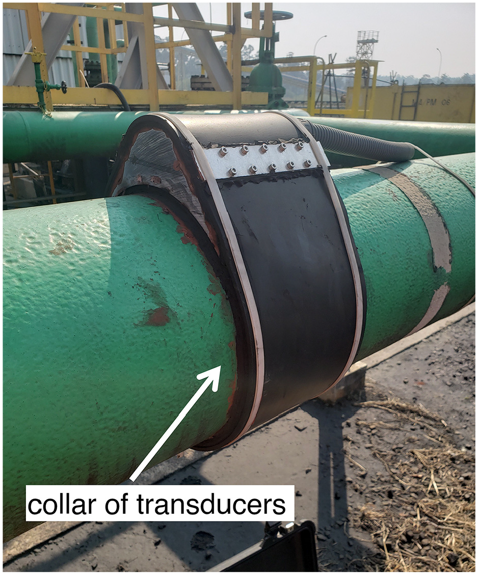
For the inspections, a collar of piezoelectric transducers was developed. The collar is composed of two independent rings, each with
The two-ring configuration, as described in the study of Oliveira HTHd, 22 aims to optimize the directionality of the inspection, allowing for a detailed analysis of wave propagation and defect identification.
The transducers used are made from modified lead zirconate titanate (PZT), model PIC255 from PiCeramics, selected for their thermal and electromechanical properties, which favor operation in dynamic systems subject to large temperature variations.
The collar was built by brazing the transducers to a fiberglass plate coated with copper, a material chosen for its flexibility and ability to adjust to the curvature of the pipe, as can be seen in Figure 1.
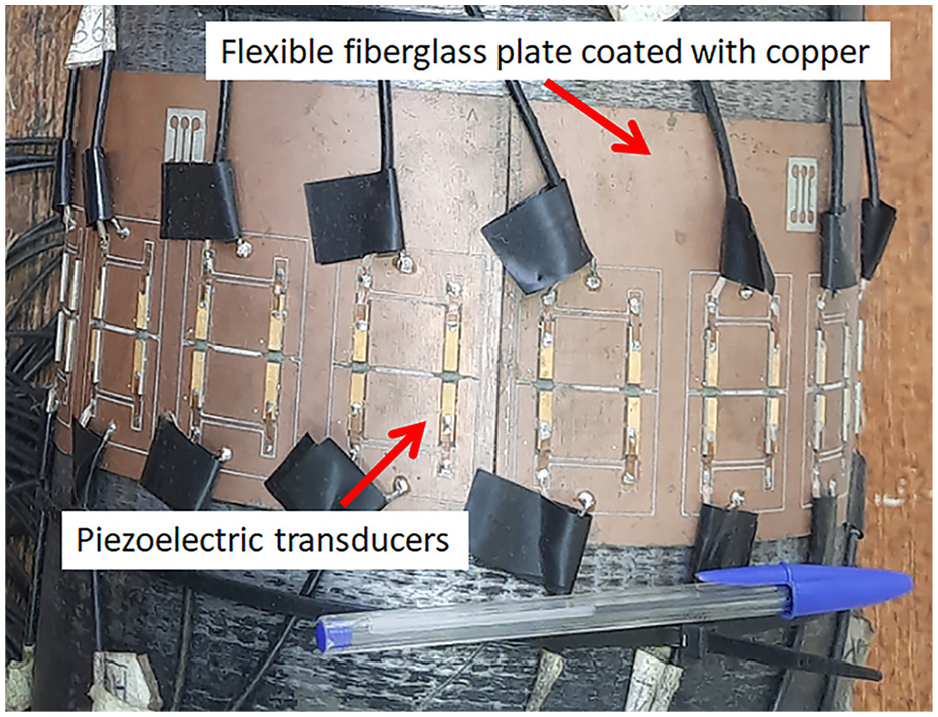
Flexible fiberglass transducer collar with a copper coating permanently coupled to the pipe.
The installation area was sanded to remove insulation, and the plate was fixed to the seam-welded steel pipe (
In the tests conducted, the pipeline was exposed and not buried. If the pipeline were buried, the primary difference would be a reduction in the propagation range of guided waves. 24 This reduction occurs due to increased energy dissipation resulting from interactions with the surrounding medium, which attenuates the wave energy and restricts its effective transmission along the structure.
The sample was placed on two metallic rollers with a diameter of
The positioning of the transducers and the corrosion site was determined after an analysis of wave propagation in a finite element model. In this model, a mesh of a pipe subjected to torsional force on its external surface was constructed, replicating the experimental conditions with the same geometry and frequency spectrum, simulating a shear piezoelectric crystal. The center of the collar was positioned
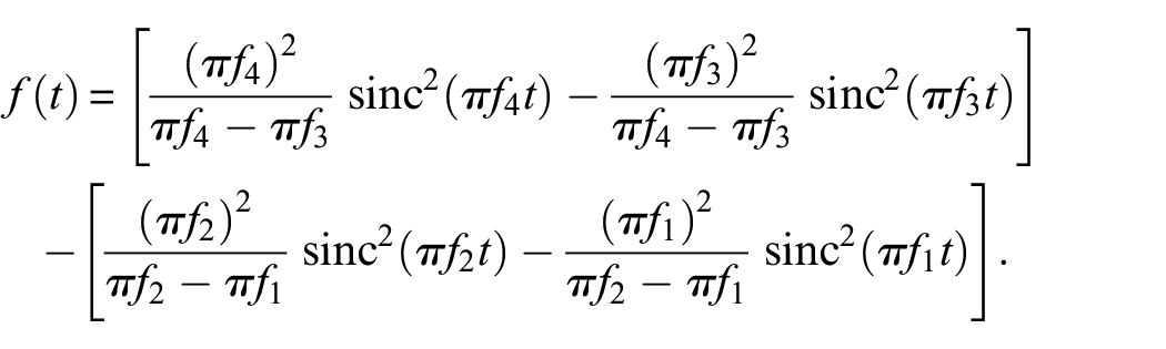
For the excitation of the piezoelectric transducers, an Ormsby-type waveform was chosen, as expressed in Equation (1),
25
generated at a frequency of
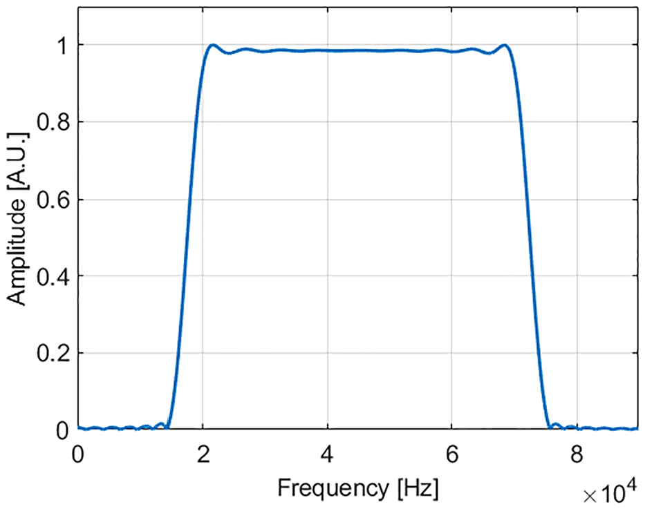
System excitation waveform—Ormsby in the frequency domain.
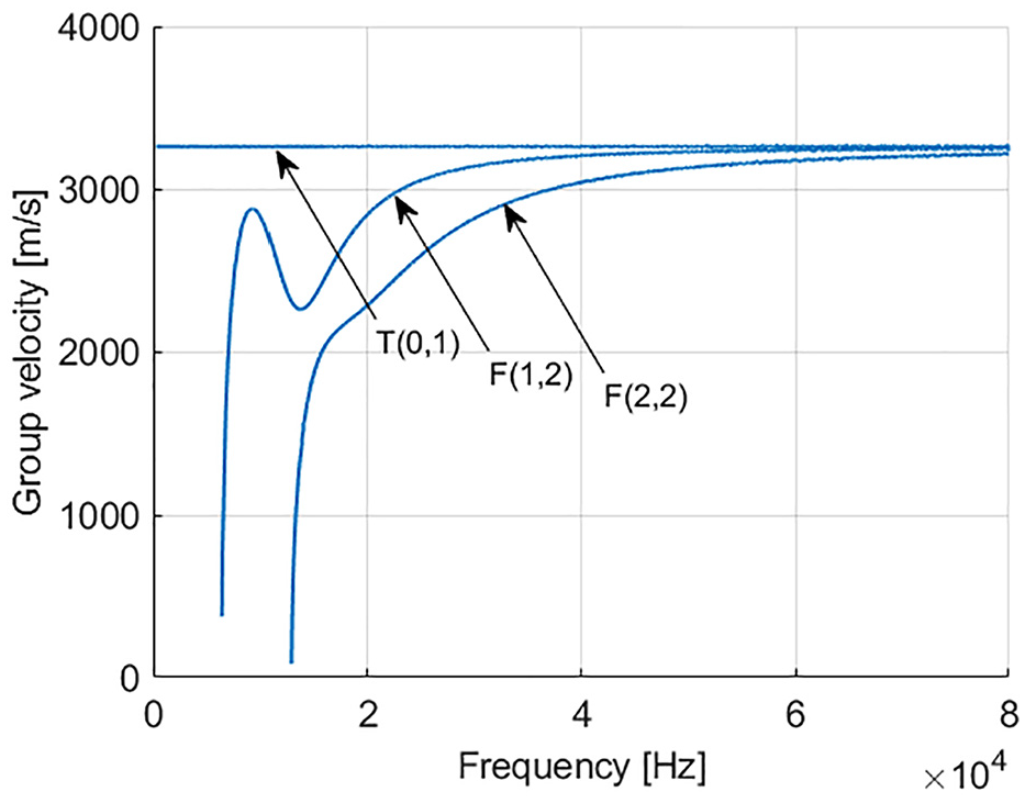
Dispersion curve for an 8-inch diameter, schedule 40 steel pipe, illustrating the relationship between wave group velocity and frequency for the guided wave modes of interest.
Controlled corrosion test
A closed electrical circuit was established by connecting the pipe as the anode and a stainless steel electrode as the cathode to a DC power supply, as can be seen in Figure 4. In this setup, a synthetic seawater solution served as the electrolyte to enable electrochemical reactions at the metal-solution interface, while the application of a constant current from the DC power supply enhanced the ionic conductivity and actively promoted controlled corrosion in the pipe region.
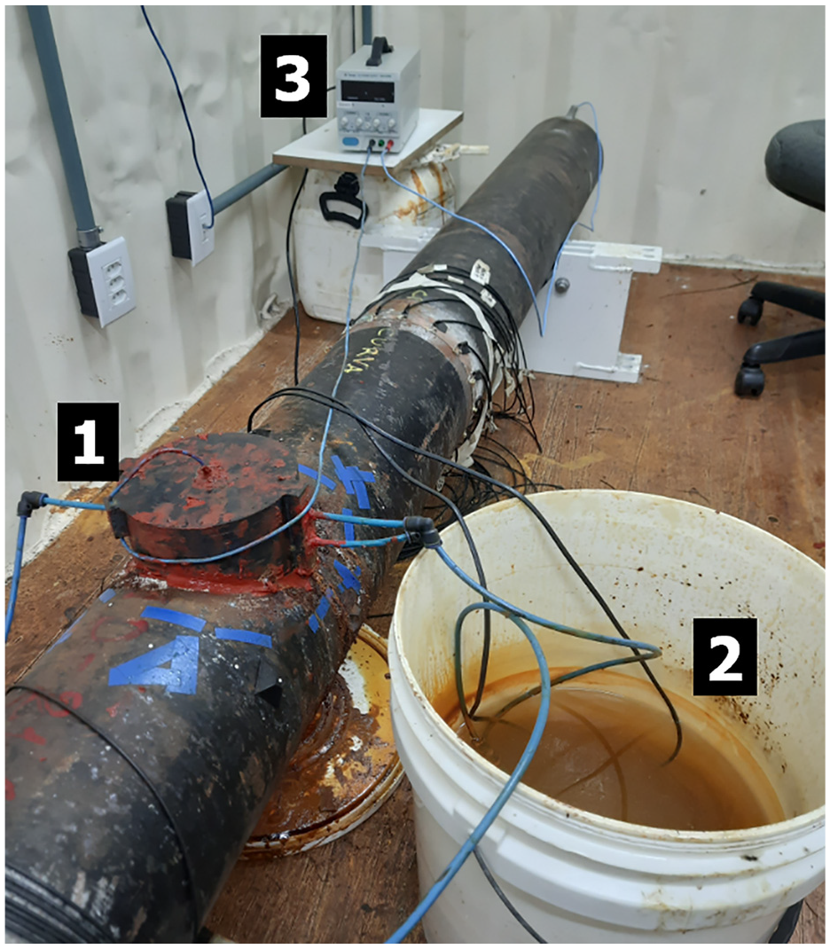
(1) Corrosion device with pumping system (2) Ionic solution (3) Direct current power supply used to force the corrosion through current control.
The corrosion device was printed in high-density ABS material, with a diameter of
Data generation and acquisition
The signal generation was performed using custom equipment, with the USB-6366 OEM board from National Instruments as the central element. This multichannel acquisition board features maximum acquisition rates of
The multiplexing circuit interconnects the sensors with the excitation and acquisition subsystems. The acquisition board has eight digitization channels, which, through the multiplexing circuit, allows for the acquisition of a total of
The signals were acquired at a rate of
The system is also equipped with four channels for temperature measurement, designed for reading sensors with a digital interface via the I2C protocol. Of these four channels, three monitor the temperature in the transducer-coupling region, contributing to thermal compensation procedures, and one monitors the relative humidity. Temperature is recorded before each data collection stage, with eight averages obtained per guided wave signal to reduce electromagnetic random noise.
The electronics of the equipment allow for voltage and electric current measurement at each transducer of the collar, enabling the evaluation of the electrical impedance. These parameters are important for analyzing the current condition of the sensors, potentially indicating component ageing in the collar or even a failure in one of the transducers.
Guided wave acquisition routine
The procedure was carried out over a period of
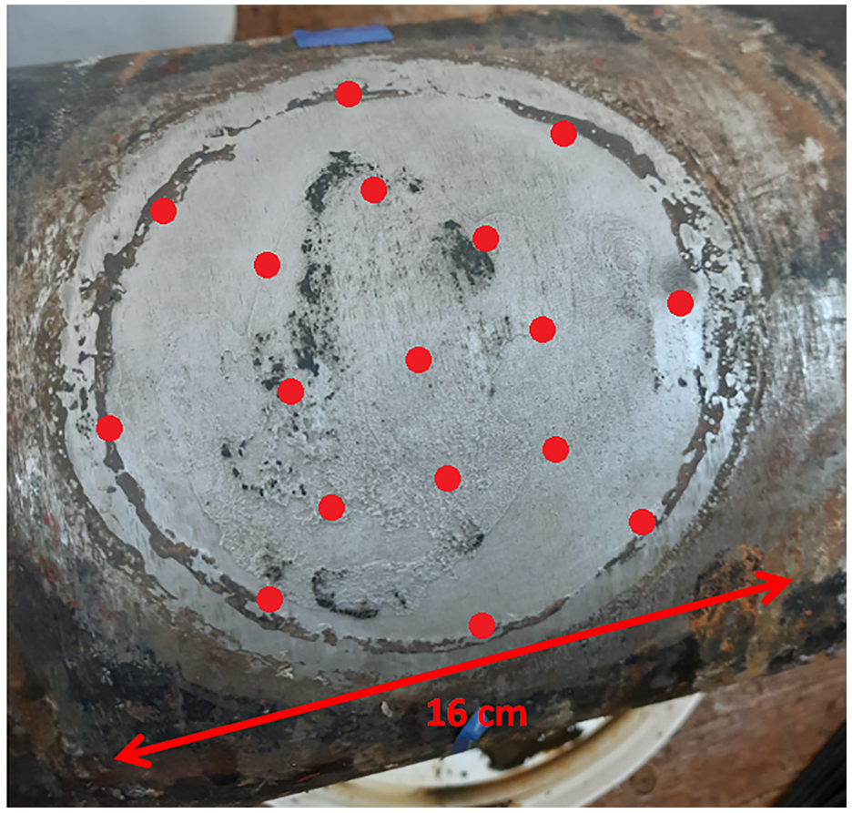
The experiment was conducted in iterative stages until a reduction of at least 50% of the pipe wall thickness was achieved, as summarized in Table 1. The abbreviation CSA refers to the cross-sectional area, representing the area of the cross-section of the pipe removed due to corrosion. In this study, CSA is an estimate based on measurements taken at 17 points, as illustrated in Figure 5.
GW signal data collected to monitor corrosion progression.
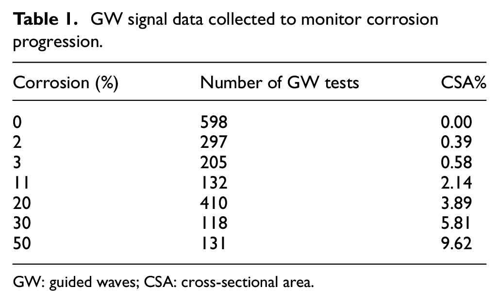
GW: guided waves; CSA: cross-sectional area.
Positions of
The cumulative thickness loss at each stage was monitored using a GE DM5E series ultrasonic thickness gauge. The corrosion area was characterized by measurements at
The signals collected by the sensors were initially subjected to a fourth-order Butterworth band-pass filter, with cut-off frequencies at
The raw data matrix is preprocessed to generate a matrix
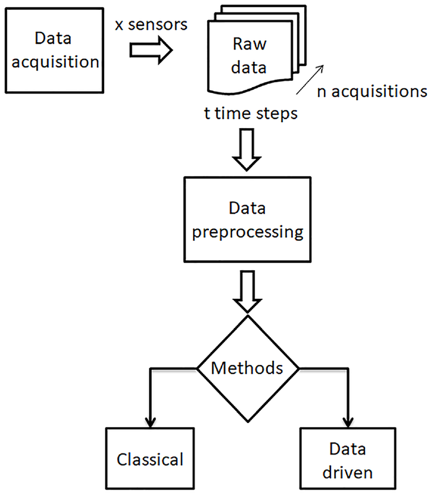
Experimental schema.
Classical SHM approach
Temperature compensation
To address this challenge, non-destructive evaluation techniques employ baseline signals as reference points. 26 An initial set of baseline measurements was acquired prior to defect introduction, and subsequently, interrogation measurements (obtained with the defect present) were subtracted from the baseline data to isolate the defect-related signals.
To mitigate thermal variation effects on the acquired signals, a series of temperature compensation techniques was applied to the data for the first three modes in the torsional family (
The variations in temperature and air relative humidity to which the system was exposed throughout the experiment are presented in Figure 7.
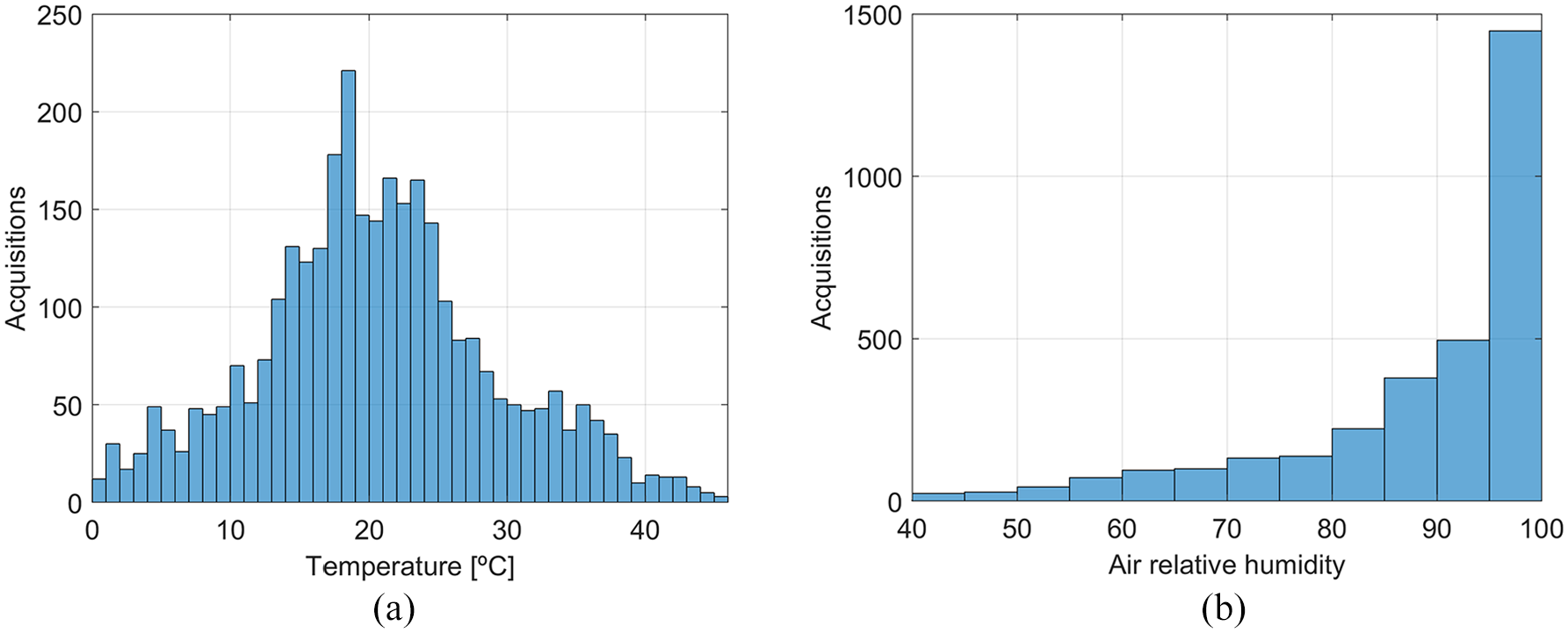
Variation of environmental conditions throughout the experiment: (a) temperature histogram for data collected along all the corrosion steps and (b) air relative humidity histogram for data collected along all the corrosion steps.
Initially, the optimal baseline selection (OBS) technique was used to select the most suitable baseline signal for comparison with the data from each corrosion stage. This technique involved subtracting the baseline signal from the acquired signal at the damaged stage, followed by calculating the root mean square (RMS) value of the resulting difference. The baseline signal that resulted in the lowest RMS value was selected as the reference for the subsequent stages.
After selecting the baseline, the baseline signal stretch (BSS) technique was applied. This method enhanced the signal-to-noise ratio and allowed the signal in the defect region to be highlighted, as shown in Figure 8. It is important to note that there are two dead zones in the signal, where no reliable information can be obtained. The first zone covers the initial region, up to approximately 1.8 m, and is affected by crosstalk and the shadow caused by reflection from the left edge. The second zone is located at the end of the duct caused by reflection and mode conversion at the right edge.
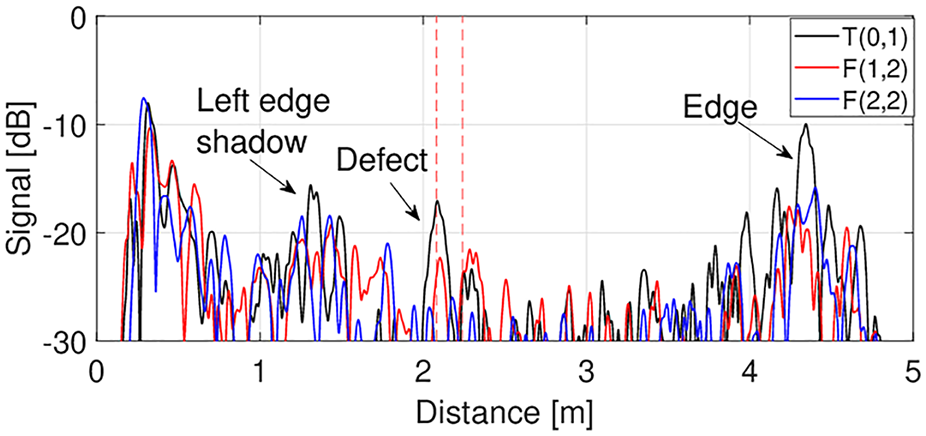
A-Scan for BSS and optimal baseline subtraction for the pipeline.
Scientific machine learning in SHM applications
With the advancement of technology and computational power, data-driven methods have become increasingly relevant in SHM,9,27 making the analysis of large volumes of data technically and financially feasible. The primary goal of these methods is to identify patterns, detect anomalies, and monitor the progression of damage as it occurs. 2
Supervised machine learning is based on establishing mappable relationships between known input and output values, where each input is associated with a predetermined target value.28,29 In SHM applications, this approach would require a large amount of data from various stages of structural damage to stablish a model and associate specific conditions with the corresponding system responses. This is unfeasible, as the actual state of the structure is often unknown, making it impossible to label or classify the data appropriately. Moreover, the model generated for a particular structure may not generalize to other structures, even if they are of similar types, due to intrinsic differences between them.30–32
To overcome these limitations, unsupervised and hybrid deep learning methodologies have gained increasing attention. For example, a deep autoencoder combined with a one-class support vector machine has been shown to facilitate accurate damage detection utilizing only baseline acceleration data for training. 33 Likewise, a density peaks-based fast clustering algorithm has been proposed to effectively detect and localize structural damage without the need for labeled data. 34 Recent advancements have further broadened the applicability of unsupervised novelty detection approaches, including comprehensive comparative analyses evaluating the performance of diverse machine learning and deep learning methods for structural damage detection. 35 These approaches exploit normal data from undamaged conditions to develop statistical models, which are subsequently employed to identify anomalies in damaged structures, such as loosened bolts in steel bridges.
Unsupervised methods are fundamentally designed to autonomously infer the probability density characteristics from the data, extracting meaningful patterns and information from its underlying structure without the need for supervisory input or labels. 36 These methods offer a distinct advantage by requiring only the creation of a comprehensive database of the structure in its undamaged state during the initial phase. This reference database serves as a baseline for comparing future conditions that may indicate potential damage or anomalies. A key benefit of this approach is that data from damaged structures are not required during the initial data acquisition.37,38 Furthermore, the elimination of the need for data labeling addresses a critical challenge in practical, real-world operational environments, where labeling can be infeasible. 38
Building on these advancements, a comprehensive review of deep learning-based SHM applications has underscored key innovations, including automated feature extraction, integration with digital twins, and computer vision techniques for detecting structural damage under diverse conditions. 39 These developments exemplify the transformative potential of deep learning in addressing traditional SHM challenges, while paving the way for more robust and scalable solutions.
Abbasi et al. 19 investigated unsupervised machine learning techniques for the SHM of a carbon-fiber–reinforced polymer (CFRP) plate embedded with piezoelectric transducers to detect and localize damage under varying temperature conditions. The study modeled reversible damage using a 10 mm-thick aluminum disc placed at four distinct locations on the plate and evaluated the performance of four dimensionality reduction algorithms—principal component analysis (PCA), kernel PCA (KPCA), t-distributed stochastic neighbor embedding (t-SNE), and autoencoder (AE)—in distinguishing structural states. Two evaluation strategies were employed: score plots (utilizing latent dimensions) and damage index (DI) plots (based on Q-/T2-statistics).
The autoencoder demonstrated superior performance in the first strategy, successfully detecting and differentiating damage locations even under temperature fluctuations, whereas PCA, KPCA, and t-SNE achieved effective damage detection only within limited temperature ranges. For the DI plot strategy, all methods effectively identified damage across all temperature conditions, obviating the need for additional temperature compensation. The findings emphasize the exceptional capability of the autoencoder for damage localization and highlight the robustness of Q-/T2-statistics for temperature-invariant damage detection.
Curse of dimensionality
The curse of dimensionality refers to a set of phenomena that arise when working with data in high-dimensional spaces. This concept was initially described by the study of Bellman 40 as an optimization problem in multidimensional spaces that demands a significant amount of computational memory due to the complexity involved in analyzing each additional dimension. When the number of dimensions is high, datasets become very sparse. 41 This occurs because, as dimensions increase, the search space expands, creating a matrix where the data are distributed more sparsely, with regions of high and low data density. This sparsity may prevent from drawing meaningful conclusions from the data. Consequently, models developed using sparse data may lack robustness, leading to over-fitting and poor generalization to unseen conditions. 42
Moreover, the concentration of measures in high-dimensional spaces diminishes the effectiveness of traditional distance metrics, such as Euclidean distance.43,44 This deterioration in discriminative power complicates the identification of proximity and similarity among data points, which is the objective of an anomaly detection system. When distances converge to similar values, it gets challenging to distinguish between normal and abnormal behavior.
Additionally, as the dimensionality of the data increases, the volume of noise introduced into the system also rises 45 and data becomes less informative. This noise can obscure the underlying patterns within the data. As a result, it compromises the capacity of accurately identifying structural issues without incurring false positives or negatives, further complicating the decision-making process when detecting damages in the structure.
Dimensionality reduction methods
Dimensionality reduction, also known as manifold learning, 46 is an area within machine learning and data-driven methods that seeks to extract relevant features from a high-dimensional dataset to better represent it or to separate distinct information. Dimensionality reduction methods serve as an exploratory analysis tool, and through them, patterns related to defects and anomalies in the underlying data structure can be found. The idea is to represent the data in a reduced dimension without losing important information, eliminating noise and redundancies. 47 Dimensionality reduction can be classified into three major categories: spectral dimensionality reduction, probabilistic dimensionality reduction, and neural network-based dimensionality reduction. 46
Spectral dimensionality reduction involves eigenvalue decomposition, having a geometric bias. This category includes PCA, Isomap, and Locally Linear Embedding (LLE), among other methods. Probabilistic dimensionality reduction, on the other hand, uses statistical models that assume the data in the high-dimensional space are governed by a smaller set of latent variables in a lower-dimensional space, representing the underlying structure of the data. According to the study of Ghojogh, 46 these methods are more robust, compared to spectral ones, in dealing with missing data.
Nonlinear dimensionality reduction methods are reduced to the task of recovering low-dimensional structures within a higher-dimensional structure and are divided into two categories: global and local. 48 Global analysis enables the identification of separation and transitions across different corrosion levels, thus reflecting the progression of the corrosion process. Local analysis, in turn, captures specific variations and anomalies within each corrosion level, aiming to detect emerging patterns in the data that may indicate potential structural integrity issues or malfunctions in the operational or transduction systems.
According to the study of De Silva and Tenenbaum, 49 the effectiveness of dimensionality reduction methods heavily depends on inherent structure of the data. The primary goal, however, is to balance the trade-off between achieving accurate anomaly detection, specifically for early corrosion detection and the computational resources required.
Three low computational cost and well-established methods were selected for analysis: one linear, PCA, and two nonlinear methods, t-SNE and LLE. This selection aims to leverage the strengths of each approach, where PCA is designed to handle linear relationships, and identify and extract principal components that best represent the patterns associated with defects. This approach seeks to minimize data complexity and to highlight aspects that are indicative of anomalies, thereby enhancing early corrosion detection.
On the other hand, t-SNE and LLE methods provide a more intuitive visualization of relationships within the data, allowing anomalies to be visually distinguished. t-SNE provides detailed data visualization despite its higher computational demands, 50 and LLE serves as a computationally economical alternative for capturing nonlinear patterns. 51 This direct visualization of anomalies in these methods can reveal patterns that may not be evident in the original data representation. Training neural-networks, however, demand significant computational resources. Although certain embedded electronics with advanced computational capabilities can support this task, the primary role of the embedded system in this context is to generate waveforms and ensure precise data acquisition. Consequently, computational resources must be allocated primarily to these critical functions, leaving minimal capacity for additional processes, such as training deep learning networks.
To optimize the performance of these methods, all parameter settings were determined heuristically, considering the unique characteristics and dimensionality transformation strategies of each approach.
Principal component analysis
PCA is a widely used statistical method for feature extraction, data compression, and as a preprocessing step.
52
The algorithm was initially proposed by Pearson
53
and Hotelling,
54
and its primary goal is to project a high-dimensional dataset
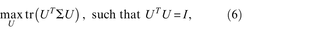
The objective of PCA is to maximize the variance of the data projected onto a latent subspace of
The centered data matrix

The covariance matrix
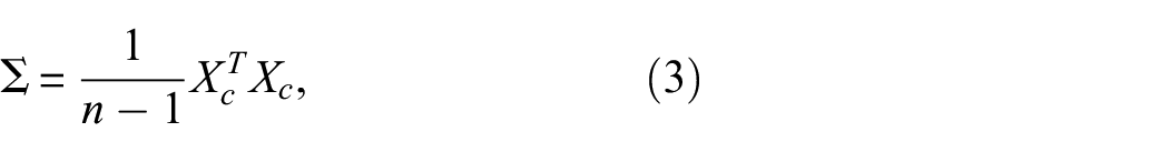
where
The next step is to project the data onto

where

where
To perform the data projection in multiple dimensions
where
In the study of Ma et al., 55 a variant of PCA is employed for monitoring defects in pipes by adaptively selecting the appropriate number of components to reduce noise and eliminate redundancy in the data.
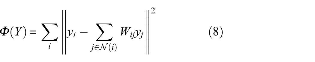
Figure 9 presents the results of PCA using two components, where the first two components are illustrated. The data projection is color-coded according to the degree of corrosion, ranging from 0% (base, intact pipe) to 50% of the average wall thickness loss of the pipe.
Dimensionality reduction for each propagation mode, utilizing PCA with two components to illustrate well-defined corrosion stages. The data points are color-coded to represent varying degrees of corrosion, with colors transitioning from 0% intact (base, intact pipe) to 50% mean wall thickness loss. (a)
Although PCA is a linear method, it still provides moderate manifold separation for the
Locally linear embedding
LLE is a dimensionality reduction method that aims to preserve the local relationships between data points when mapping them from a high-dimensional space to a lower-dimensional space.
Although LLE is a nonlinear method, it assumes that each data point can be represented as a linear combination of its nearby neighbors. 56 The global coordination of these local linear models, introduced in the study of Roweis et al., 57 allows for the smooth modeling of high-dimensional data in a global coordinate system, promoting the seamless integration of multiple local linear models into a single global representation in reduced dimensions, particularly useful during unsupervised learning, where the structure of the data is unknown a priori.
LLE identifies the
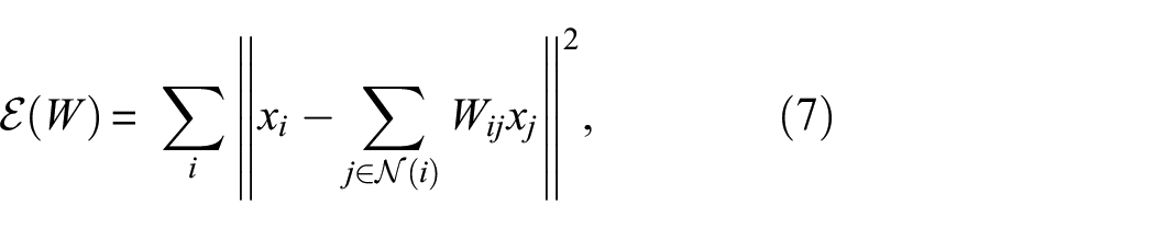
where
After calculating the weights
To find the low-dimensional configuration that best preserves the neighborhood relations from the original space, this cost minimization can be converted into an eigenvalue problem.
58
In this context, the matrix
In Figure 10, the results of the LLE are presented. It is evident that, under the configurations used, for discrete corrosion stages, the
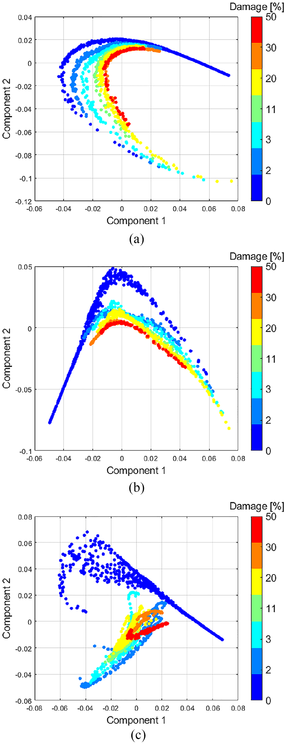
Dimensionality reduction using LLE with 50 neighbors for all wave propagation modes. Data points are color-coded to indicate corrosion levels, ranging from 0% to 50% average wall thickness loss. (a)
Although there is no clear explanation for the superior performance of the
By adjusting the hyper-parameter that defines the number of neighbors, which determines how many nearby points are used to reconstruct the local structure in the lower-dimensional projection, it is possible to enhance the resolution for this mode. However, such a modification might degrade the resolution for the other modes.
T-Distributed stochastic neighbor embedding
t-SNE is a dimensionality reduction technique that is particularly effective for visualizing high-dimensional data in a two-dimensional or three-dimensional space. The method is widely used for visualization and exploratory analysis, and it performs excellently compared to other methods such as Isomap and LLE, particularly in preserving the structure of clusters. 60
In addition to preserving local structure, t-SNE is reasonably effective at capturing the global structure of the data, representing broader relationships between data groups. As noted by Maaten and Hinton in their study, 61 the use of a t-Student distribution to calculate point similarities in the low-dimensional space allows for the modeling of larger distances more effectively, preventing points that do not belong to the same cluster in the high-dimensional space from being placed close together in the reduced dimension.
t-SNE optimizes the Kullback–Leibler (KL) divergence between the two similarity distributions, one in the high-dimensional space and the other in the reduced dimension, which allows the method to capture local relationships between points and maintain relative distances between similar points in the lower dimension. 62
Additionally, Kobak and Berens 63 show that using PCA on the data as a starting point for t-SNE can improve the balance between global and local relationships, and Agis and Pozo 64 use principal component reduction via PCA before applying t-SNE. Although PCA is a linear algorithm and may not fully capture complex nonlinear structures, it may still provide a useful initialization for t-SNE, which subsequently refines the data projection to preserve local relationships, but should be used with caution in order not to compromise the analysis.
According to Maaten and Hinton,
61
the algorithm begins by modeling the similarities between data points in the original high-dimensional space using Gaussian probability distributions. For each pair of points
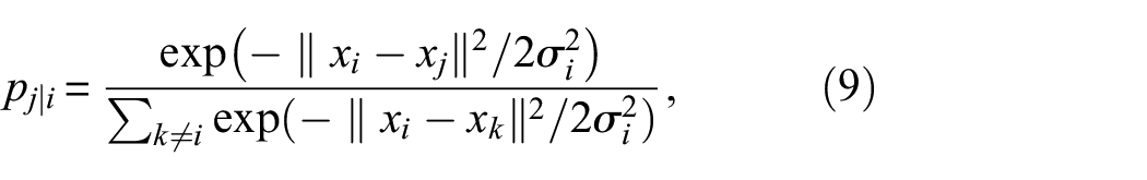
where
In the low-dimensional space, the similarities between points
Then, t-SNE minimizes the KL divergence between the distributions
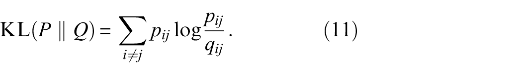
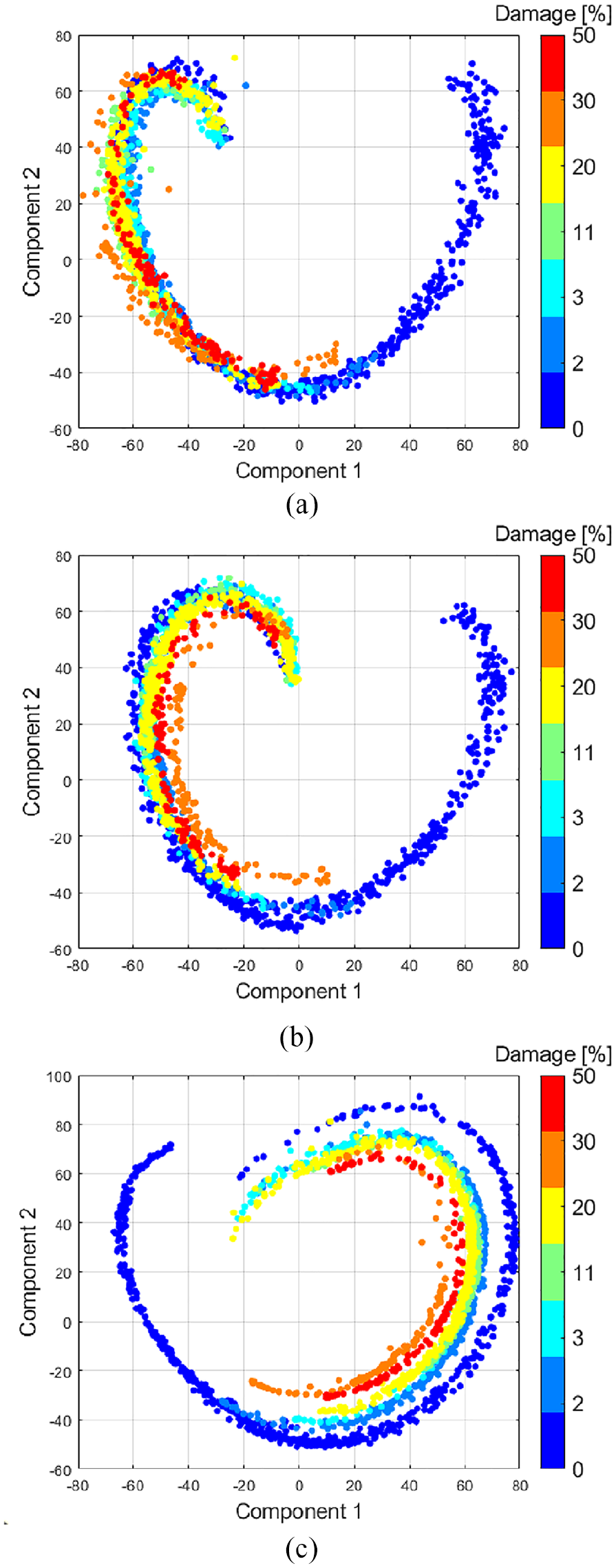
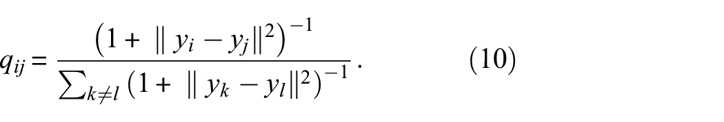
The t-SNE method prioritizes the preservation of the local data structure as can be seen in Figure 11, where it is possible to identify the formation of well-defined clusters, with minimal overlap between the data points. However, it introduces distortion in the global structure, resulting in apparent nonlinearity in the spacing between clusters representing different levels of corrosion.
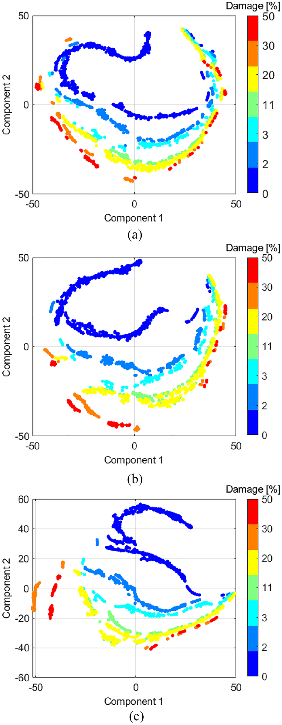
Dimensionality reduction using t-SNE with perplexity adjusted to
t-SNE is effective in representing local structures but has limitations in representing global structures. This implies that inter-cluster distances may not have real significance, potentially leading to misleading interpretations. 65 As observed, the relative distance between clusters corresponding to 2% and 3% average thickness loss is greater than the distance between 30% and 50%.
By maintaining local relationships, the signals corresponding to the same corrosion level remain close in the reduced dimension, facilitating cluster identification. However, preserving global relationships ensures that the overall configuration of clusters in a high-dimensional space is maintained in low-dimensional space, following a reasonably consistent order of corrosion progression.
Empirical observations indicate that when multiple stages of corrosion are present, local differences tend to be “squeezed” or “compressed.” Notably, there is a tendency for the manifold to become uniform, even when only baseline data are considered. This phenomenon can be influenced by the choice of perplexity or the number of neighbors, parameters that are inherently linked to the distances between data points. Given that t-SNE and LLE emphasize local relationships, they may highlight local properties inherent in the baseline data, such as specific anomalies within a determined corrosion level that tends to become obscured when numerous corrosion stages are present. Consequently, if only defect-free data are included, there is a potential risk of misleading the inspector into perceiving these highlighted characteristics as defects.
SHM and parsimonious representation
Figure 12 illustrates the progression of various estimators used for corrosion damage assessment. The figure presents the traditional SHM approach (depicted by solid gray lines) alongside reduced-dimensional representations derived from PCA, LLE, and t-SNE, shown as blue, red, and black lines, respectively.
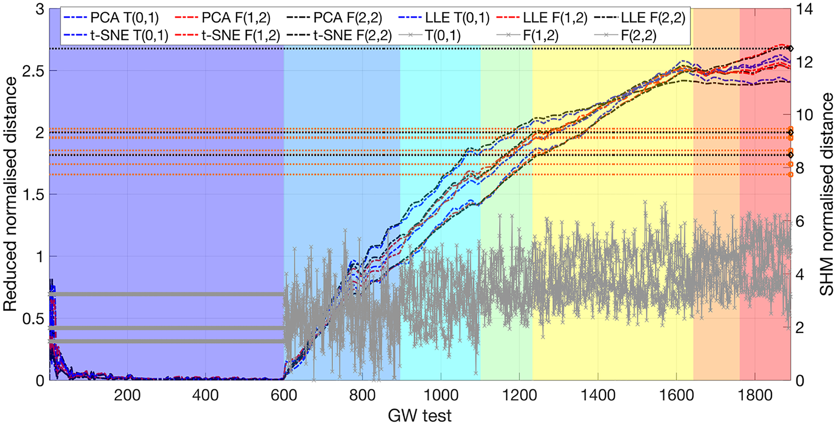
Normalized estimators for corrosion damage are shown here. The solid gray lines represent the classical SHM approach. Among the dimensionality reduction methods, the solid line corresponds to the LLE method, the dashed line to PCA, and the dash-dotted line to t-SNE. The
To facilitate a meaningful comparison between the SHM data and the data-driven methodologies, all datasets were normalized to a standard normal distribution
After normalization, a classical
It can be clearly observed that this outlier detection metric is not effective in identifying defects when analyzing the combined OBS + BSS data. However, when reduced-dimensional data are utilized, the algorithms demonstrate the capability to detect defects. In the worst-case scenario, defects as small as approximately 4% of the CSA were detected. Conversely, in the best-case scenario, using
Additionally, it is evident that the normalized distance metric fluctuates during the initial data collections. This behavior is attributed to the influence of temperature, which impacts the stability of the system and the formation of the initial support manifold. This phenomenon will be addressed in detail in the subsequent section.
The estimator for the classical SHM approach is simply the maximum value in the defect region. This indicator reveals that, despite effective temperature compensation, a significant level of noise remains in the signal. A clear trend of increasing estimator levels can be observed as corrosion severity escalates; however, noise may interfere with accurate corrosion identification.
The estimator used for the dimensionality reduction methods is described as follows: each point
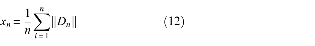
where
The employed method does not provide spatial localization of corrosion but instead serves as an estimator of the signal trend over time, enabling the identification of deviations that suggest the need for further investigation. This approach aligns with the foundational level of the framework proposed by Burgos et al. 67 (illustrated in Figure 1 of Burgos et al.’s study). Once damage is identified, specific localization methods can be employed, such as the Common Source Method described by Davies. 68
Given the continuous nature of the damage monitoring process, the presence of outliers does not compromise the ability to identify damage. Instead, it is more critical to observe consistency and discernible trends in signal behavior over time. This becomes particularly apparent when comparing the reduced noise achieved through dimensionality reduction methods to classical SHM data, which benefits from the capacity of these algorithms to filter out noisier components, such as through truncated singular value decomposition (SVD). 69
This approach is especially significant in embedded systems, where the local processing unit requires a well-defined threshold to detect anomalies. Establishing such thresholds ensures the system avoids generating false positives, thereby preventing unnecessary alerts for system operators.
Temperature influence
Figure 13 illustrates how data-driven algorithms can distinguish environmental effects from structural anomalies without requiring compensation algorithms. The clustering patterns highlight this differentiation. Component 1 shows a strong temperature influence, while corrosion levels exhibit radial distance among them, indicating the ability of the method to differentiate between temperature-driven variations and structural changes. Each dimensionality reduction method uniquely captures these influences, effectively isolating temperature and corrosion effects in the data.
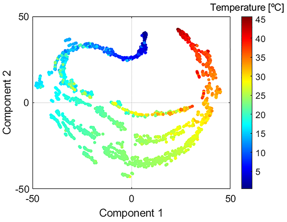
t-SNE for wave mode
Although it is possible to separate the thermal effects from those caused by damage, temperature still has a significant impact on the data structure, similar to traditional inspection techniques. Qualitatively, it can be observed that extreme temperatures tend to make it more difficult to distinguish between damage levels. This difficulty in distinguishing corrosion levels at extreme temperatures may arise from the unequal distribution of data across different damage levels. While it is not possible to definitively ascertain the specific cause of this issue, studies 19 indicate there is a temperature range where inter-cluster separation is more evident.
System change detection
To evaluate the capability of the methods in detecting system changes, two transduction channels were intentionally damaged during the last two phases of data acquisition. The integrity of the connections and transducers was ensured through the analysis of individual capacitances throughout the data collection stages, as illustrated in Figure 14 for a temperature of approximately
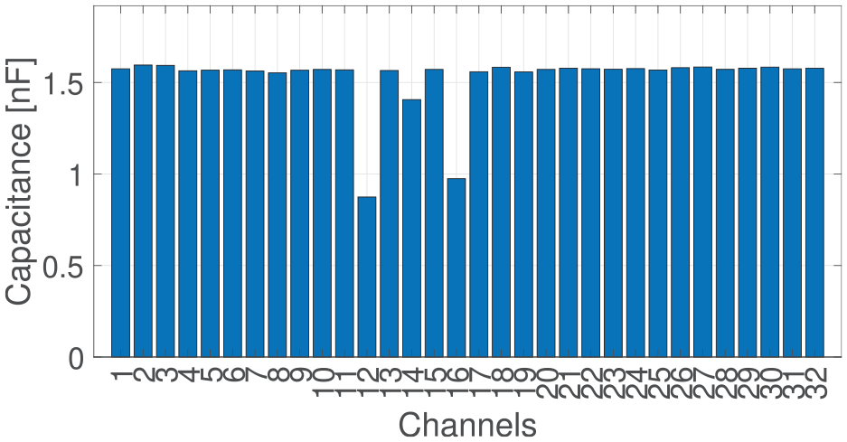
Integrity check for 32 transduction channels at 25°C. Capacitance at 200 kHz with channels 12 and 16 damaged.
In this figure, it is visually possible to differentiate the abrupt change in the capacitance of the damaged channels compared to the others. The measure was performed at 200 kHz to enhance sensitivity to capacitive variations. These changes are greater than those caused by thermal fluctuations.
The deterioration of the transduction channels occurred after reaching 53% of average wall thickness loss in the pipeline. Initially, channel
The deterioration of channel
The results indicate the capability of the t-SNE method (Figure 15) to detect changes in data structure associated with transduction loss. This is evidenced by the significant separation of clusters that occurs as the transducers degrade. The method effectively captures subtle structural changes, particularly in the context of the collar containing
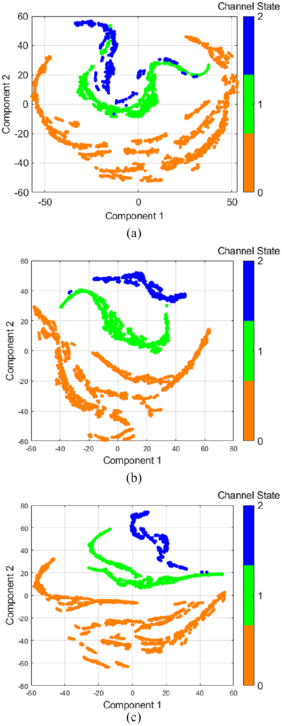
Dimensionality reduction using t-SNE with a perplexity of 30, illustrating well-defined corrosion stages and the impact of damaged transduction channels. The data points are color-coded as follows: 0 indicates all channels intact, 1 represents one damaged channel, and 2 denotes two damaged channels. (a)
Field application in a refinery
The system developed in this work was designed as a digital twin of a SHM system installed in an oil refinery. It served multiple purposes, including validating the methodology and results obtained from field tests. However, its primary objective was to evaluate the method under a new set of environmental conditions. Care was taken to produce two systems that incorporate identical materials and transduction technologies, both installed on pipelines of matching diameters. This ensures that only the environmental conditions differ between the two systems.
The refinery system was installed in December 2022 and operated until September 2024, during which approximately 41 GB of data were collected and transmitted via wireless communication to a centralized storage and analysis hub (Figure 16).
System installed at the refinery. This system serves as a twin to the one described in this study and incorporates wireless communication for remote data transmission to a central storage and analysis unit.
The collected data were analyzed using classical and data-driven methods, with no anomaly indicators detected. Figure 17 shows the t-SNE of the T(0,1) mode, where clustering patterns remained consistent throughout the operational period, indicating the absence of damage.
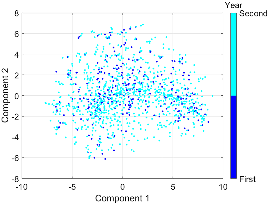
t-SNE visualization of the refinery data, using two components and color-coded by year of operation. The absence of any indicators of damage over the 2 years of monitoring is demonstrated by the clustering patterns, which remain consistent throughout the operational period.
The environment in a refinery is highly aggressive for equipment, with a significant presence of electrical and mechanical noise. Nevertheless, the installed system has demonstrated robustness, withstanding the adverse operational conditions of a refining unit without the need for frequent maintenance.
Figure 18 demonstrates that, following the methodology used for the laboratory system, no defects were identified in the pipe. Data from 2022 were adopted as the pristine state for the calculations. Initially, the same phenomenon observed in Figure 12 can be seen, where the system undergoes a natural transition between low and high temperatures. This behavior is attributed to the significant influence of temperature on the manifold,
70
as further illustrated in Figure 13. Subsequently, as the temperature cycles stabilize, the values also stabilize with minor fluctuations. After the first year, around test 270, small oscillating fluctuations are observed. However, these remain within the established threshold based on the
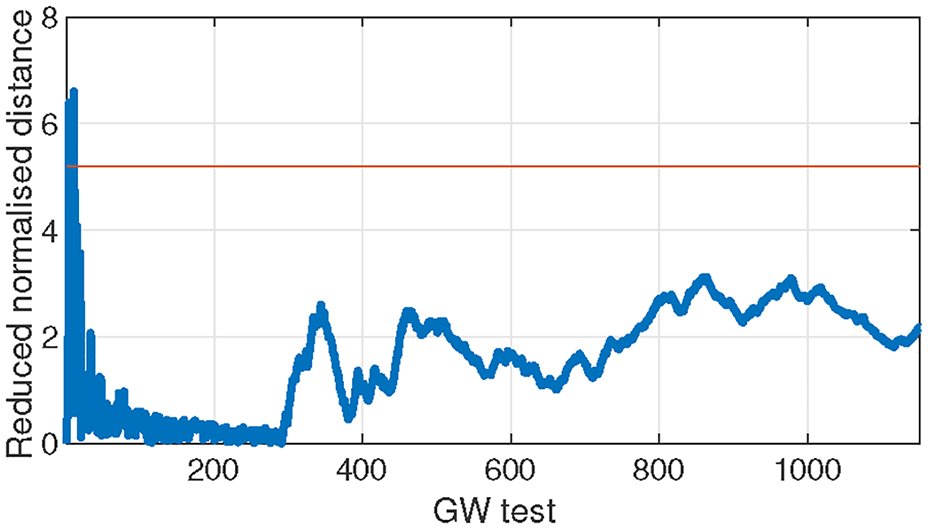
The normalized reduced-dimension data from guided wave tests are represented by the solid blue line, while the orange horizontal line indicates the outlier detection threshold based on the
Conclusion
An electrolytic corrosion test was conducted on an 8-inch diameter pipeline to evaluate its structural integrity and detect signs of corrosion. This method employs an electrolytic solution that, upon contact with the pipeline material, allows for the observation of the behavior of the metal under simulated corrosion conditions. A classical structural health monitoring analysis using guided waves, applied to the pipeline after the test, confirmed the presence of corrosion and demonstrated effectiveness in early-stage identification of such damage.
Various data reduction techniques (PCA, LLE, t-SNE) were applied to the guided wave modes
By applying a historical average to the dimensionally reduced data, a smoother variation in the data was observed. Furthermore, both linear and nonlinear techniques produced comparable results across the modes
The physical twin, deployed in a refinery under real-field conditions, demonstrated remarkable stability over a 2-year period, with no significant variations detected. This consistent behavior serves as a robust baseline, suggesting that no damage has occurred within this time frame. The role of the physical twin is crucial in providing continuous, real-time data on the operational integrity of the structure in its actual environment. By replicating the system in a controlled yet realistic setting, the twin allows for ongoing monitoring, validating that the structure remains unaffected by external stressors or corrosive agents that could otherwise lead to degradation or failure.
This study demonstrates the feasibility of establishing a threshold for autonomous anomaly detection using an extensive corrosion dataset from oil pipelines, including laboratory and field tests. Results show that CSA losses as small as
Additionally, the findings validate the scalability of computationally efficient dimensionality reduction algorithms for embedded systems with hardware and connectivity constraints. These algorithms enable early corrosion detection, supporting predictive maintenance strategies that optimize schedules, reduce unnecessary interventions, and improve structural asset management.
Footnotes
Acknowledgements
The authors would like to thank the Brazilian National Agency for Petroleum, Natural Gas and Biofuels (ANP) and Petrobras for providing the resources for this project. Prof. Dr. Thomas G.R. Clarke would like to acknowledge funding provided through the CAPES-PROEX Program of PPGE3M and through the productivity scholarship provided by CNPq.
Declaration of generative AI in scientific writing
During the preparation of this work the author(s) used ChatGPT in order to improve the readability and language of the manuscript. After using this tool/service, the author(s) reviewed and edited the content as needed and take(s) full responsibility for the content of the published article.
Declaration of conflicting interests
The author(s) declared no potential conflicts of interest with respect to the research, authorship, and/or publication of this article.
Funding
The author(s) received no financial support for the research, authorship, and/or publication of this article.