
Abstract
In industrial equipment fault diagnosis, different components of various equipment exhibit diverse motion forms and intensities, leading to significant differences in the variation patterns of vibration signal parameters across components. Under interference, both the trend information and the transient information of signals are affected by noise. This results in signal blurring and overlapping, making it challenging to characterize the multimodal nature of the signals. Based on this, the paper proposes a decoupled learning with a reduced convergence domain (DL-RCD) method. First, an innovative Haar wavelet attention operator is introduced, which decouples different frequency features in complex pattern signals, effectively narrowing the convergence domain of network operation parameters. Second, the proposed multifeature extraction operator constructs a process of horizontal and vertical functional interaction mapping. This ensures that when extracting coupled features, the model’s long-term operational trends are not disrupted by short-term transient features. Third, the proposed joint measurement model can analyze the correlation between the macro characteristics and detailed information of the signals. In addition, the constructed scale correction fusion module explores the joint encoding of channel and feature scale dimensions, reducing the negative impact of interference information on decision-making. Since DL-RCD enforces the model to focus on specific frequency bands where fault features reside through frequency domain attention, it reduces the influence of irrelevant information and noise, thus maintaining efficiency even with small and diverse datasets. This general model offers greater advantages in industrial scenarios by simplifying maintenance processes and reducing the number of models that need to be managed and updated, especially in situations where edge computing device resources are limited.
Introduction
In power plants, rotating machinery is the main auxiliary equipment for production, and its operation directly affects whether production can proceed safely and stably. Vibration signals are an important means of detecting the status of equipment and overcoming and solving the problem of fault diagnosis based on vibration signals is helpful for the efficient monitoring and maintenance.
For a long time, extensive efforts have been made on how to extract various fault feature information from mechanical vibration signals.1,2,3 Li et al. 4 proposed a fault-type identification method based on symbolic dynamic filtering for early fault detection and intrinsic characteristic scale decomposition. Xie et al. 5 designed a method involving bandwidth empirical mode decomposition and adaptive multiscale morphological analysis applied in bearing fault identification. Wang et al. 6 conducted a statistical spectral analysis based on the state of rotating motors, classifying the amplitude of the spectral content of vibration signals and converting them into statistical spectral images. Deng et al. 7 established a serial principal component analysis method with integrated features and utilized a similarity factor method for fault identification. The analytical methods guided by professional domain knowledge can effectively enhance the interpretability of decisions.
The quality of feature extraction determines the identification performance. Researchers are dedicated to enhancing model feature extraction quality to improve diagnostic results. Deng et al. 8 proposed a motor-bearing fault diagnosis method that integrates fuzzy entropy and support vector machines based on fault feature extraction and theoretical calculations with empirical wavelet transform and Hilbert transform. Hu et al. 9 presented a method using wavelet packet decomposition and kernel principal component analysis combined with a weighted extreme learning machine to effectively improve diagnostic accuracy. Zhang et al. 10 designed a weighted minority oversampling method and utilized a deep autoencoder approach to enhance fault diagnostic effectiveness. The signal processing method significantly improves the accuracy and efficiency of equipment fault diagnosis through multidimensional feature decoupling and intelligent algorithm collaboration.
Currently, data-driven and knowledge-based end-to-end intelligent methods are considered excellent tools for fault diagnosis.11–13 These methods utilize deep learning frameworks to directly process raw vibration signals or operational data, eliminating the intermediate steps of manual feature extraction and signal transformation found in traditional approaches. The model parameters are automatically updated based on data distribution to capture sensitive and subtle features of equipment faults. In addition, the model exhibits cross-domain generalizability, providing effective support for system decision-making in intelligent operations and maintenance. Xie et al. 14 proposed a new multi-task attention guided network, suitable for multi-objective fault diagnosis. Su et al. 15 suggested adding a branching structure to one-dimensional CNNs to allow hierarchical diagnosis of bearing faults through multiple output layers. Yang et al. 16 developed a multi-branch deep neural network, where each branch was designed to process a specific type of fault data. Huang et al. 17 proposed a deep adversarial capsule network that integrates multi-domain generalization into intelligent compound fault diagnosis. For the decoupling problem of compound faults. Huang et al. 18 utilized an ensemble learning model based on deep capsule networks. Chen et al. 19 constructed a self-supervised knowledge-embedded autoencoder network using prior knowledge from a multiscale convolutional autoencoder to provide an effective solution for fault diagnosis.
The above-mentioned fault diagnosis methods can be categorized into three forms: (1) analyzing signal characteristics using signal processing methods, (2) performing feature extraction after signal processing analysis, and (3) highly adaptive feature learning models. The analysis method of signal processing relies on professional domain knowledge to extract the physical features of signals, which is suitable for application scenarios with limited data volume but has limited feature expression ability. Deep learning models can automatically dig abstract features, but they are prone to overfitting when data is insufficient, making it difficult to fully utilize their advantages. The learning modes of mutually stacked independent methods are prone to conflicts due to different rules. Therefore, consider the joint optimization of embedded. Li et al. 20 explored the advantages of wavelet capsule networks in compound fault diagnosis. Li et al. 21 introduced the wavelet kernel network to obtain a customized kernel bank for extracting fault-related impact components. In the scheme proposed by Wang et al., 22 the Haar wavelet convolution extraction module was used for synchronously mapping features at different frequency scales, conducting multilevel, multiscale analysis of fault signals, and jointly extracting temporal, frequency, and spatial information to enhance the model’s robustness and generalization capability. The fusion of wavelet prior knowledge with deep learning overcomes the spectral limitations of traditional convolution. However, using continuous wavelet transform to initialize the extraction of local detail excitations in signals lacks global exploration, as the wavelet basis function dictates the width of the features extracted by the model and limits the diversity of the extracted features. Although Wang et al. 22 performed a global wavelet process; it lacked deep spectral attention, which may lead to functional failure after multilayer extraction.
Although these methods attempt to provide a connection between device fault types and signal characteristics through powerful learning capabilities. However, in practical engineering, the motion forms and intensities of component information from different faults vary, and the patterns of change in vibration signal parameters for various components will also differ significantly. This results in signal blurring and overlapping phenomena, making it difficult to characterize the multimodal nature of the signals. Under interference, both the trend information and the transient information of signals are affected by noise. Existing advanced deep learning methods attempt to extract discriminative features from signals using various attention mechanisms. However, under conditions of multisource coupling, the feature extraction components require a larger and more cumbersome parameter search domain, which may find suitable information, undoubtedly increasing the model’s convergence difficulty, convergence time, and computational complexity. This also necessitates a larger volume of data and hardware resources for training. Multiple channels of fault features gather fault components from different modes, and these signal components are often sensitive to specific scales. Considering that some discriminative periodic components may carry high-frequency features such as transient impacts or pulse excitations, and knowing that traditional multiscale operations tend to map features as a whole, which generally relies on convolution kernels with significant differences or multiple convolution layers. Therefore, traditional multiscale functions struggle to observe complex local and global coupled information at low computational complexity. The deeper the model processes the signal, the more it extracts the overall operational trend information of the equipment. These macroscopic features, which represent the equipment’s state, are highly discriminative but also lack detailed information, limiting their higher analytical capabilities. This is a primary factor why current model performance cannot fundamentally break through the designated baseline, and thus, using these features alone may lose the model’s ability to analyze subtle faults. Feature selection is crucial for the final analysis. A lack of selection functionality causes the model to generate a lot of redundancy while imposing greater classification weight calculations on other irrelevant information elements and minor feature scales, significantly increasing the likelihood of model misjudgment.
Based on the above motivations, this paper proposes a decoupled learning with reduced convergence domain (DL-RCD) to enhance the model’s diagnostic capabilities in complex environments. First, an innovative Haar wavelet attention operator (HWAO) is proposed, which simply decouples different frequency features in complex mode signals, effectively narrowing the convergence domain of network operation parameters. Meanwhile, due to the prior spectral feature domain, it is possible to analyze the discriminative features and interference information at different frequencies in detail within a small parameter interval. Second, the proposed multiscale feature enhancement operator (MFEO) strategically constructs a process of horizontal and vertical functional interaction mapping, where layered multiscale learning and step-by-step integration functions can use multiple local small receptive fields to expand the model’s receptive area while, when extracting coupling features, ensuring that long-term operational trends are not disturbed by short-term transient features. In addition, vertical encoding of the importance parameters of different feature domains aims to understand the degree of discrimination in different modal components. They can enhance the learning ability of discriminative features without increasing additional computational load. Third, the proposed joint measurement module (JMM) can analyze the correlation between macroscopic features and detailed information of signals, solving the numerical solution of the parameters’ simultaneous equations of deep and shallow features, making it easier to project useful information into the discriminative feature domain. It is the core of the overall multiscale analysis in DL-RCD. Furthermore, the constructed scale correction fusion module (SCFM) explores the joint encoding of feature channel dimensions and scale dimensions, efficiently mapping discriminative features while reducing the negative impact of interference information on decision-making, ensuring model performance. DL-RCD joint measures multifunctional mapping sets, constructing various learning domains for detailed study of fault feature expression. The specific contributions are as follows:
The proposed HWAO introduces a set of adaptive wavelet learning functions using Haar wavelet transformation, integrating wavelet prior knowledge while effectively decoupling modal components in complex vibration signals. It meticulously learns discriminative features across different frequency intervals.
The proposed MFEO is a novel multiscale extraction and step-by-step integration strategy, allowing two different functional mechanisms to encode each other, accurately expressing transient impacts, pulse excitations, periodic components, and other detailed information and long-term operational information in composite signals.
The constructed SCFM can jointly encode time-frequency coupled spatial and scale features, ensuring the stability of the model’s expression of discriminative features.
The proposed DL-RCD consists of HWAO and MFEO as encoding units for feature extraction; JMM is an important component of the selection unit for correlation analysis; SCFM serves as the fusion unit, organizing decision information. It forms multiple feature learning domains, involving fault feature layer-by-layer abstraction, multifrequency joint, and scale analysis schemes, enabling the model to learn more classification attributes.
Methodology
In this section, we delve into the details of the proposed DL-RCD. The structure of DL-RCD is shown in Figure 1. The DL-RCD mainly consists of five parts: the coding unit (CU), the expansion unit (EU), the selection unit (SU), the fusion unit (FU), and the diagnostic unit (DU). The CU contains several HWAO and MFEO. The EU includes several upsampling layers and interacts with the CU. The SU comprises several JMMs and integration layers. The FU includes an SCFM. The DU eliminates the fully connected layers, instead opting for convolutional decision-making. The core idea of DL-RCD is distributed learning, refined expression, and correlation analysis. The proposed CU’s HWAO employs Haar wavelet transformation and full time-frequency attention (FTFA) mechanism to form a set of adaptive wavelets learning functions, integrating wavelet prior knowledge. At the same time, it decouples different frequency features in complex pattern signals, reduces the convergence domain of network operating parameters, and effectively learns target features in different frequency domain intervals. The MFEO utilizes multiscale convolution to map different feature sets to different learning domains, using domain-adaptive vectors for deep tuning, effectively representing signal discrimination information scattered across different learning domains. The EU’s upsampling progressively provides different sizes of deep features, combined with shallow features for expressing multiscale features. In addition, the SU’s JMM can compute the correlation between CU and the EU. The inter-information between multiple mapping units is characterized, able to multiple aspects adjust the weight output of multiple learning domains. The SCFM of FU deep encodes and fuses the space features of the signals and scale features of the model, jointly representing the overall mapping characteristics of the network. The DU maps different fault states with extremely low computational complexity. Specifically, first, the signals from the sensors undergo multiscale, biased learning of fault features within the CU. At this point, the EU performs hierarchical information expansion, while the SU jointly adjusts the feature output. The spatial and scale correction mechanisms within the FU further generate the decision vector. Finally, the convolutional layer in the DU, combined with Softmax, outputs the state results, completing the diagnosis.
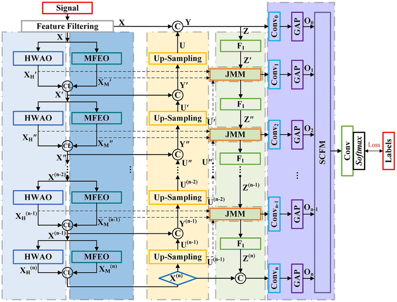
DL-RCD structure diagram.
CU: top-down approaches
The powerful tools of the CU are the HWAO and MFEO. The input signal data, denoted as X, initially passes through the feature filtering layer for preliminary feature mapping and noise filtering, resulting in features X = [x1, x2, …, xC] ∈ ℝW×C. These features are then processed using both HWAE and MFEO to learn different aspects of the features effectively, expressing discriminative information across various feature domains.
Haar wavelet attention operator
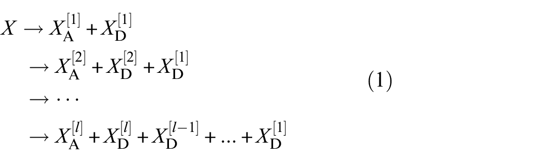
In the HWAO module, displayed in Figure 2, the focus of Haar wavelets is on expressing high and low-frequency features. Considering the first HWAO as an example, it begins by performing multilevel Haar wavelet decomposition on the input features X, obtaining several high-frequency detail features and a set of low-frequency approximate information. Assume we perform l-level wavelet decomposition, and the specific process is as follows.
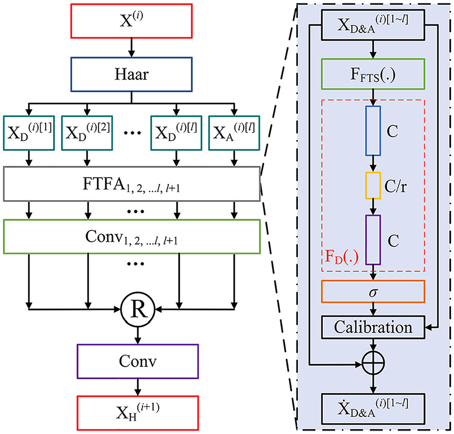
HWAO module structure.
Among them, XD[1], XD[2], …, XD[l−1], XD[l] represent all the detail coefficients obtained by performing 1, 2, …, l − 1, l levels of wavelet decomposition on X; XA[1], XA[2], …, XA[l] represent the approximate coefficients obtained after wavelet decomposition of levels 1, 2, …, l. Please note that the approximate coefficients of each level are further decomposed from the approximate coefficients of the previous level. Next, taking the first level wavelet decomposition process as an example, we will explore in detail the decomposition process of wavelet algorithms as follows:
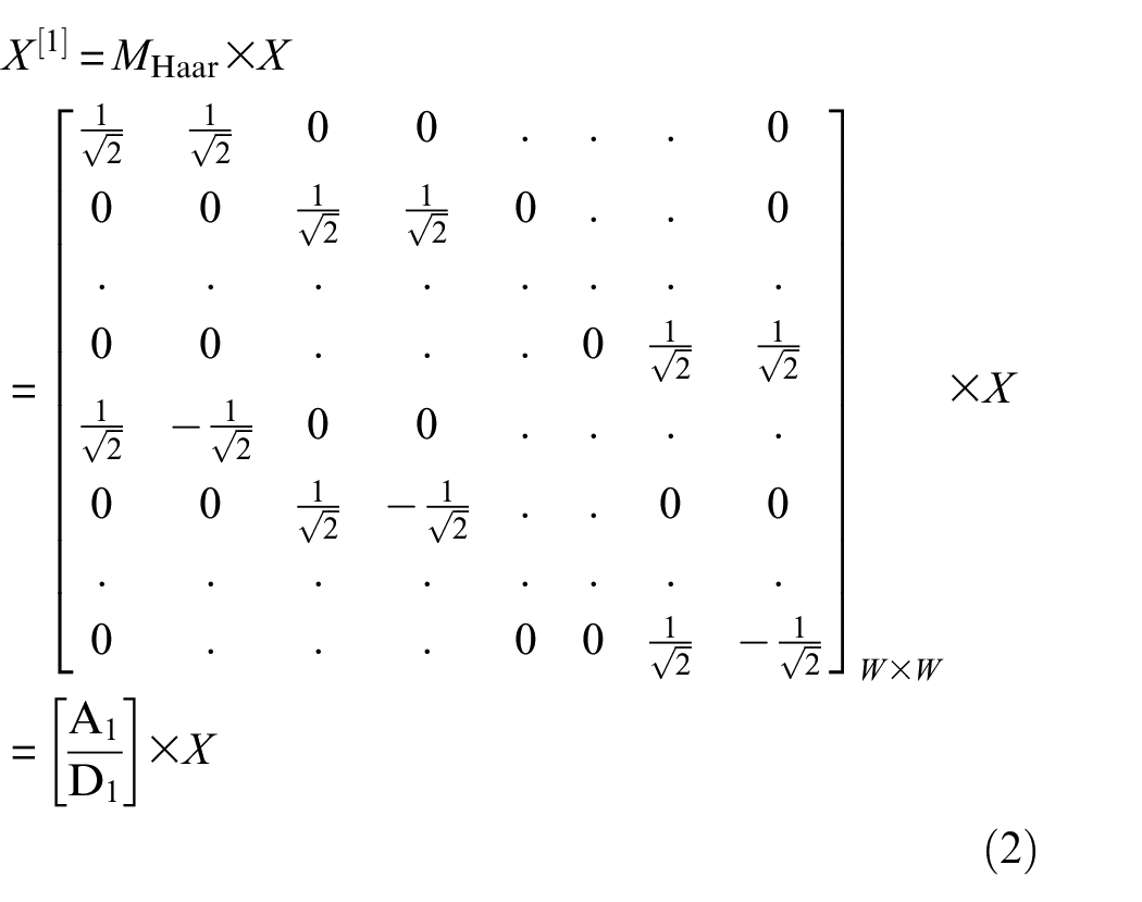
where X[1] ∈ RW×C is the feature matrix after first-order wavelet decomposition, and MHaar ∈ ℝW×W is the Haar filtering matrix, the above equation can be written as:
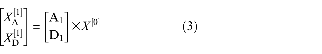
where X[0] = X, [XA[1]/XD[1]] = X[1], A1, D1 ∈ ℝW/2×W. If not limited to first-order decomposition, after the first step of wavelet transform, we retain the detail coefficient XD[1] and continue to perform wavelet transform on the approximation coefficient XA[1]:
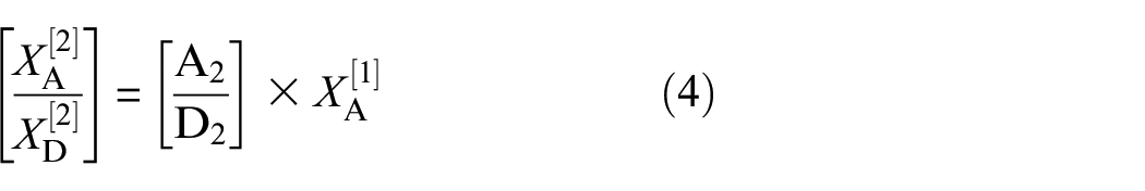
where A2, D2 ∈ ℝW/4×W/2. By analogy, it is progressively decomposed into one approximation coefficient and multiple detail coefficients. The more decomposition stages there are the finer the signal details that can be observed, which is very useful for capturing subtle changes. However, this also results in increasingly coarse information for the low-frequency components. Therefore, besides setting the number of decomposition stages for balance, we need to lean more toward adjusting the frequency spectrum importance characteristics of the features to enhance their discriminative ability. For this reason, we use FTFA to perform full-time scale and self-weighted multifrequency encoding on the decomposed detail coefficients and the approximation coefficients of the last stage. In addition to effectively capturing frequency spectrum importance elements, a full-time scale mapping rule is also constructed. Assume that the set of features after the l-th order wavelet transform are XD&A[1∼l] = {XA[l], XD[1], XD[2], …, XD[l] ∈ ℝW[l]×C, ℝW[1]×C, ℝW[2]×C, …, ℝW[l]×C, W[l] = W/2 l }. Then, using the full-time scale compression function FFTS, a full-time domain-multifrequency domain feature set is constructed. Subsequently, this feature set is deeply encoded using a set of distributed mapping functions FD, and frequency domain weight values are synthesized using a probability function. The mapped features set XD&A,att[1∼l] are generated.
Specifically, the elements XA[l] = [xA,1[l], xA,2[l], …, xA,C[l]] are encoded via Equation (5).
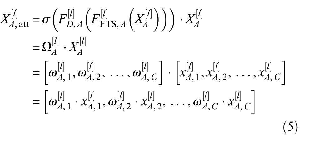
where XA,att[l] is mapped feature; σ represents the Softmax activation function, which maps data to the probability space (0,1), ΩA[l] is the generated frequency weight matrix, and ωA,1[l], ωA,2[l], …, ωA,C[l] are the weight values corresponding to different channels. Moreover, a residual connection is introduced to prevent over-response of deep features during feature weight calibration. Therefore, the frequency domain weight feature output is
among them,
Multiscale feature enhancement operator
To obtain outstanding recognition results, we build multiple paralleling learning domains, and let them encode multiscale features with less computational complexity. Meanwhile, in the other direction, we construct a sparse domain weight vector for guiding the mapping process of different learning domains, MFEO module structure in Figure 3. In the lateral information flow within the MFEO structure, the output feature map of the preceding layer, denoted as X(i)∈ℝW×C, serves as the input feature map for the MFEO. Initially, X(i) is segmented into β equal subsets along the channel dimension, represented by
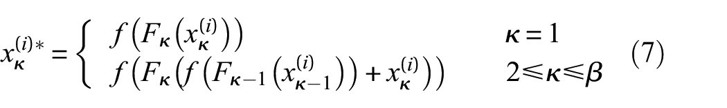
MFEO module structure.
Among them, f is the activation function. Next, we cascade these β paths, and the overall output is
Among them, concat is a merge operation. For the vertical information flow of MFEO, first perform intra-domain projection Fd on the feature X(i) divided into β subsets to obtain the domain vector Xd(i) = [xd,1(i), xd,2(i), …, xd,β(i)]. The Fd execution process is as follows:
where

Next, a more discriminative domain space is constructed to guide the learning of domain features at different scales. We recode X(i)*. In the meantime, the multiscale domain features are connected to the outputs. This residual method is used to ensure the execution stability of the module. The construction process is as follows:

Here, X(i)** represents the reconstructed output of X(i)*. Finally, the output feature XM(i+1) of the MFEO is obtained through cross-channel interactions of the integrated layer features. The integrated layer is a 3 × 1 convolutional layer (stride = 2) that can fully extract the features and reduce the dimension.
The above is a detailed description of the two functional modules of the CU. After this, the two feature maps are integrated to effectively combine information at different scales. For i-th layer features XH(i) and XM(i), the combined outcome is X(i) = CL(XH(i), XM(i)), where CL(·, ·) = Fpw(concat(·, ·)), Fpw is pointwise convolution. Then it is encoded several times in the same way, and the final output of CU is X(n).
EU: bottom-up approach
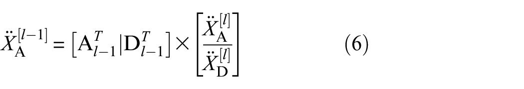
In the model, HWAO and MFEO are used at each encoding level to effectively extract fault information. It is well known that feature extraction is a continuous abstraction process, 23 which can lead to the loss of subtle fault details in low-resolution signals, such as minor cracks, wear, and corrosion. In addition, short-term impacts and transient vibrations may be smoothed out. For example, slight amplitude fluctuations generated by gears or bearings during operation, which could be early indicators of faults, may go unnoticed. Therefore, upsampling operations are often necessary to enhance these details. To keep computations simple and avoid blurring edges and details, we apply “linear” interpolation for upsampling, with a stride of 2. The designed EU further improves the temporal and frequency resolution of the fault signals, helping to capture these subtle changes and aiding the model in achieving better recognition performance. In addition, the EU echoes the multiscale learning in the CU, allowing the model to make timely use of the enhanced multiscale information, which contributes to improving the model’s robustness. Moreover, a shortcut connection is established between corresponding positions in the encoder and decoder, effectively fusing deep and shallow information to represent discriminative features at different scales. We make X(n) = Y(n), Y = Z, and the representations of the forms □, □′, □″,…are equivalent to □(0), □(1), □(2), …. Assuming that the m-th layer upsampling is in progress, the running process is as follows:
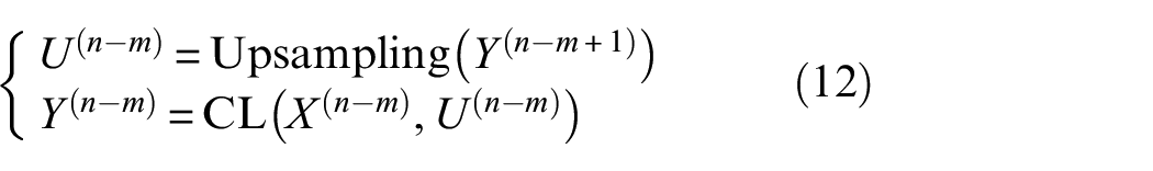
Among them, upsampling (.) is an upsampling operation; the final output of the EU is Y.
SU: lateral connections
The JMM module in the SU is designed to identify resonant information between shallow and deep features, and the structural diagram is shown in Figure 4. Deep features tend to understand the overall structure of vibration signals and their long-term correlations, revealing the time-varying spectrum characteristics within the signals. These features can express dynamic behaviors associated with device faults. On the other hand, shallow features focus on the fundamental frequency components of the vibration signal, their harmonics, and transient changes, while also capturing fine details in the signal that may contain early indications of faults. Therefore, solving the numerical solution of simultaneous equations between deep and shallow feature parameters makes it easier to project useful information into the discriminative feature space. The integration function FI aims to analyze and integrate the fused multiscale features and related information. FI is a convolution with a small kernel and few channels. The input for the SU at the i-th layer is Z(i), i = 1, 2, …, n−1.
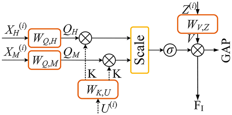
JMM module structure.
JMM and the self-attention learning mechanism of the Transformer are similar, 24 but JMM focuses on the joint representation of different queries and the queried data. Each extracted feature map is considered as a whole. We map each segment of the feature CU as query matrix Q, with HWAO and MFEO corresponding to the generation of QH(i) and QM(i), respectively; the EU is mapped as a key matrix K, and the output of the layer-by-layer integration function FI is mapped as the information carrier V, defined as follows:
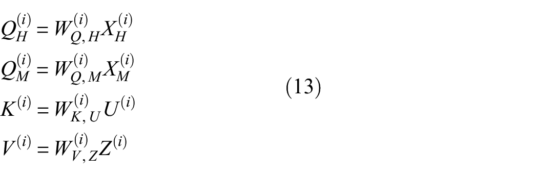
Among them,
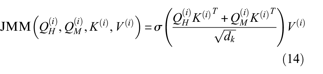
The core concept of JMM is to enable the model to autonomously learn the associations and importance between different scales of information through the functional data between the CU and EU. Its primary advantage lies in feature alignment and information transfer, effectively mapping detailed information. Through interactions with the CU and EU, JMM can consider deep, shallow, and fused information simultaneously, thus better capturing long-distance dependencies across different mapping units. In addition, JMM effectively enhances the mutual information across multiple mapping scales. 24 The outputs of JMM are directed toward two paths: the input for the FI in the next layer and toward direction of global average pooling.
Fusion unit
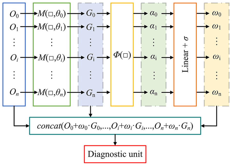
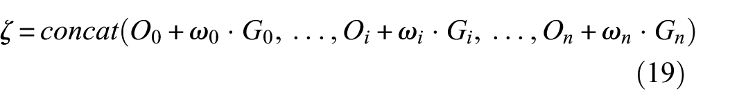
In the FU, we have developed a joint attention fusion mechanism called SCFM, in Figure 5, which can more flexibly integrate different information sources and induce spatiotemporal feature components. According to the Figure 5, the feature vectors learned from the sub signals extracted from the CU, EU, and SU are O0, O1, …, O i , …, O n , and then the features G0, G1, …, G i , …, G n are obtained through the function M (□, θ). M (□, θ) is defined as follows:
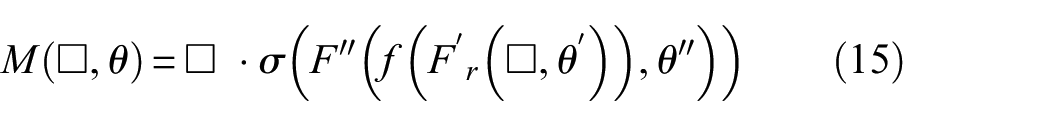
G i is obtained as follows:

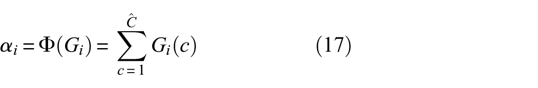
where Fr′ and F″ are 1 × 1 convolutions, r is the mapping rate, and the parameter θ is a generalized representation of θ′ and θ″. M(□,θ) focuses on the importance of the different feature dimensions among the effectively interacting elements while searching for the manifestation of discriminative information in the channel location. Then, the function Φ processes the feature group G0, G1, …, G i , …, G n to obtain α0, α1, …, α i , α n :
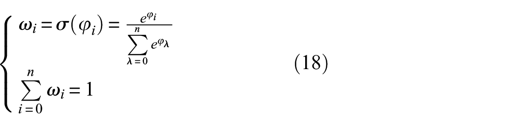
where G i (c) is the feature of the c-th channel in G i . Then, the fully connected layers “Linear” and σ are constructed to map out the feature weights ω0, ω1, …, ω i , …, ω n at different scales, which are obtained by Equation (18) computation:
SCFM structure.
Among them, φ i is the output of the fully connected layer. After integrating O i , G i , and ω i and their related features, the following results are obtained:
The DU consists of a 1 × 1 convolution and a Softmax function, with the number of convolution kernels being the diagnostic category. For specific diagnostic processes, initially, signals from sensors are input into the CU for multiscale, biased learning of fault features. At this time, the EU performs level-by-level information expansion and uses the SU to jointly adjust feature output. The spatiotemporal correction mechanism in the FU further generates decision vectors. Ultimately, the DU, with its convolutional layers paired with Softmax, outputs the state results, completing the diagnosis.
Experiment validation
Introduction to experimental data
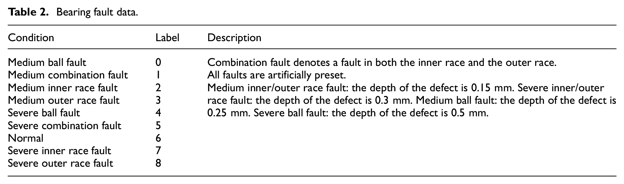
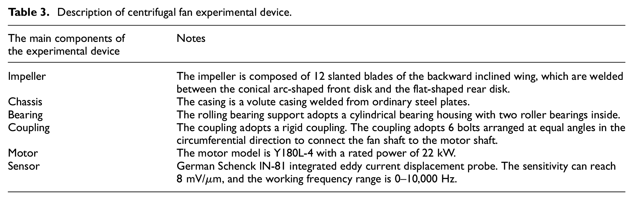
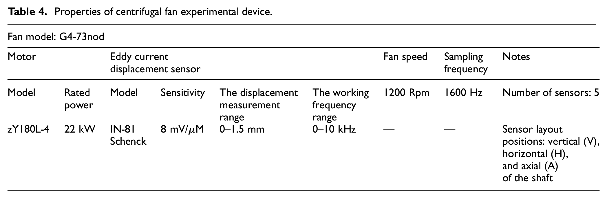
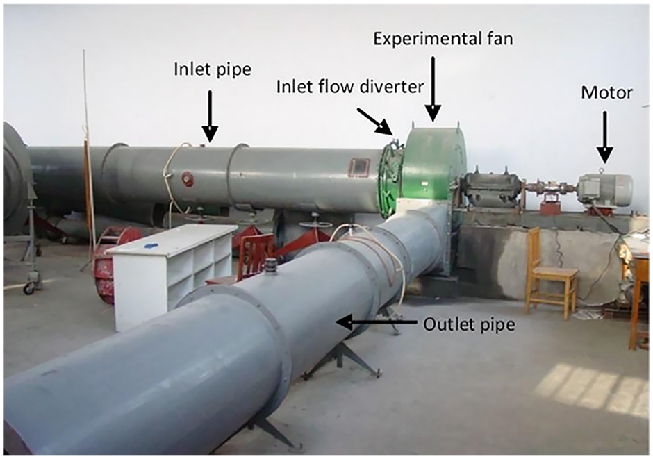
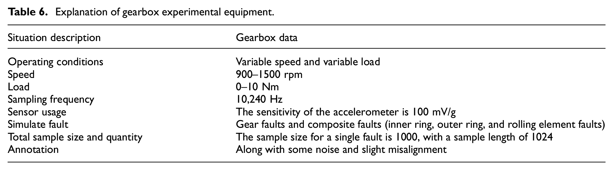
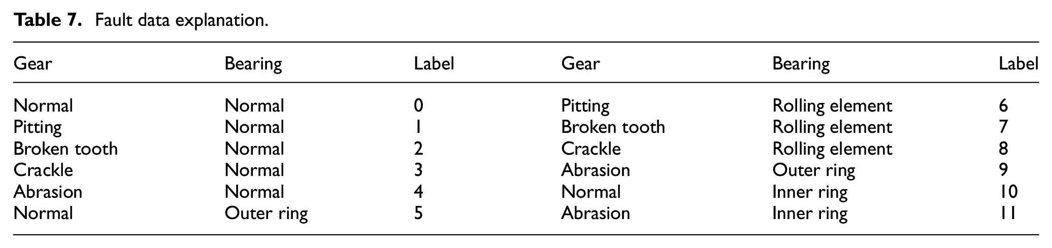
To highlight the effectiveness and generalizability of DL-RCD, we utilized the bearing public dataset from Huazhong University of Science and Technology, the centrifugal fan dataset, and the gearbox dataset with composite faults from North China Electric Power University to verify the universal performance of the model in equipment fault diagnosis25,26,27,28. For bearing data, the experimental setup and bearing fault kit are shown in Figures 6 and 7. The test-bearing model is ER-16K, and the detailed parameters are shown in Table 1. The Spectra Quest mechanical fault simulator was used for data collection, with a sampling frequency of 25.6 kHz and a length of 262,144 for each fault data. There are a total of nine device states, as shown in Table 2. Figure 8 shows the process of shifting from 0 to 40 Hz. Our data input sample length is set to 1024. To ensure that the sample contains at least a complete fault cycle, we only select vibration data within the speed range of 25–40 Hz. The total length of the reconstructed household data is 96,005, and the dataset is enhanced through overlapping sampling. For the centrifugal fan data, the detailed information is as follows: experimental equipment is shown in Table 3, experimental device performance is shown in Table 4, and fault type data is shown in Table 5. The fan experiment diagram is shown in Figure 9, and the sensor installation diagram and fan structure are shown in Figure 10. For the composite fault data of the gearbox, specific details of the experimental facilities are introduced in Table 6 and Figure 11. The fault sample parameters and corresponding labels are shown in Table 7. The fault kit is shown in Figure 12.
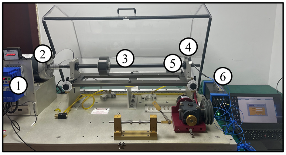
Bearing experimental device 1: Speed control, 2: Motor, 3: Shaft, 4: Acceleration sensor, 5: Bearing, 6: Data acquisition board.
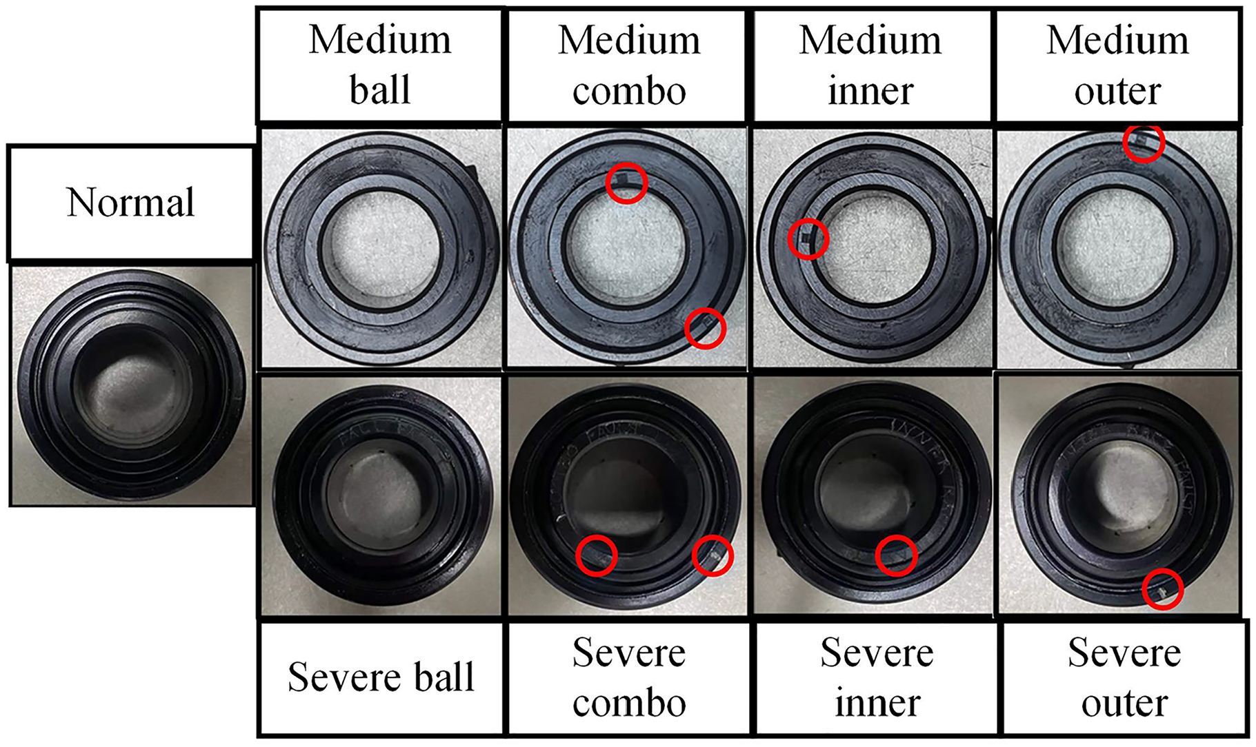
Bearing fault kit.
Er-16k bearing parameters.
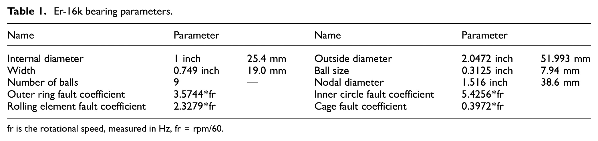
fr is the rotational speed, measured in Hz, fr = rpm/60.
Bearing fault data.
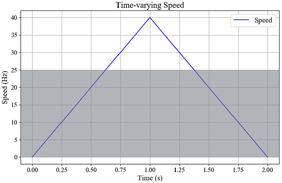
The rules governing the bearing speed variations over time.
Description of centrifugal fan experimental device.
Properties of centrifugal fan experimental device.
Fault status descriptions.
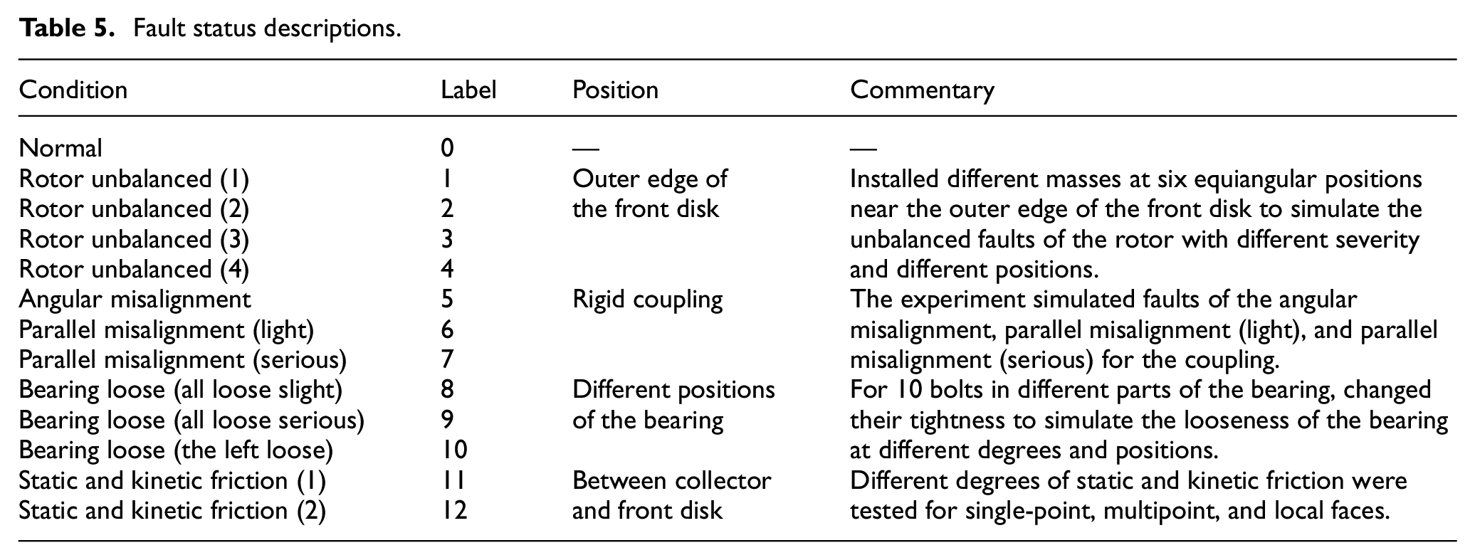
The fan of G4-73NoD.
(a) Measuring point location and (b) schematic diagram of the fan structure.
Explanation of gearbox experimental equipment.
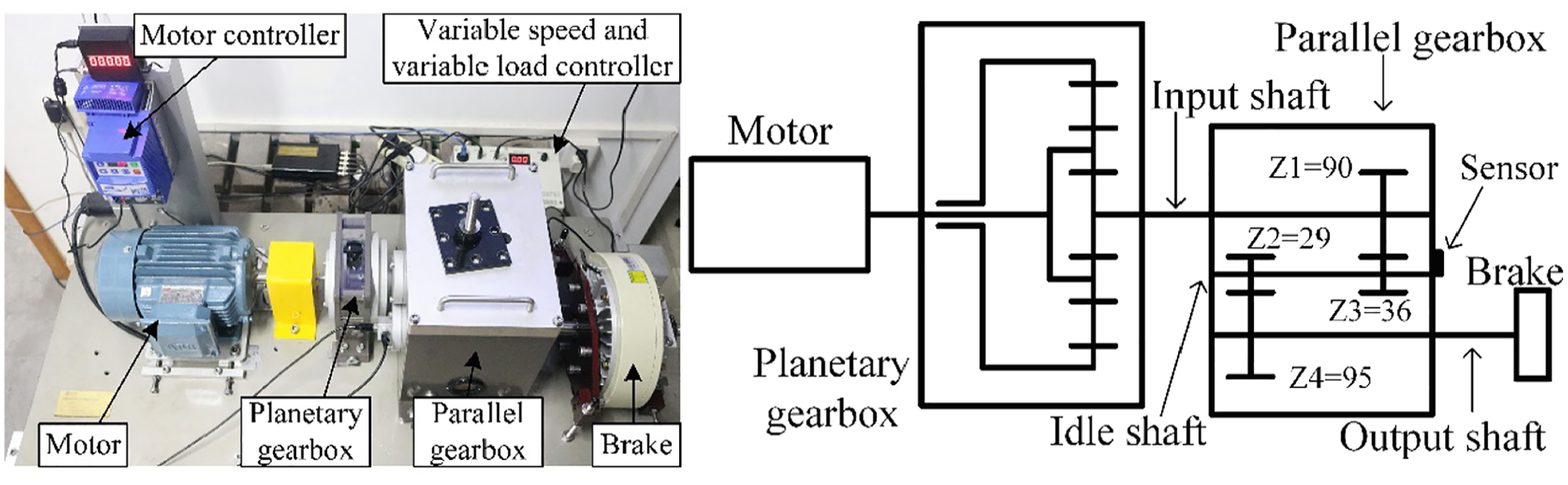
Gearbox experimental device.
Fault data explanation.
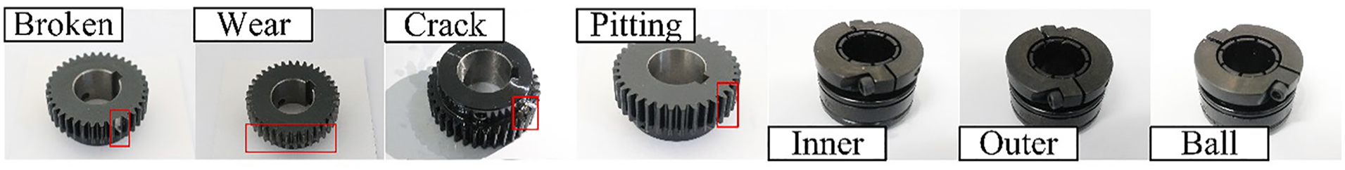
Gearbox fault kit.
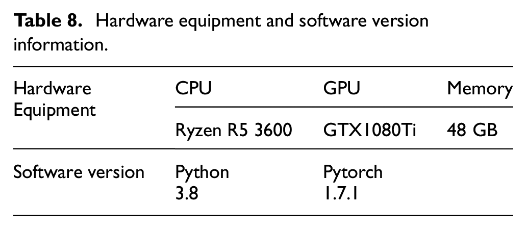
We understand that different hardware and software, as well as their versions, can have varying impacts on experimental results. To better demonstrate the effectiveness and innovation of the proposed model, we have disclosed the information in Table 8, and we use classic evaluation metrics to perform a quantitative analysis of the model, with specific parameters listed in Table 9.
Hardware equipment and software version information.
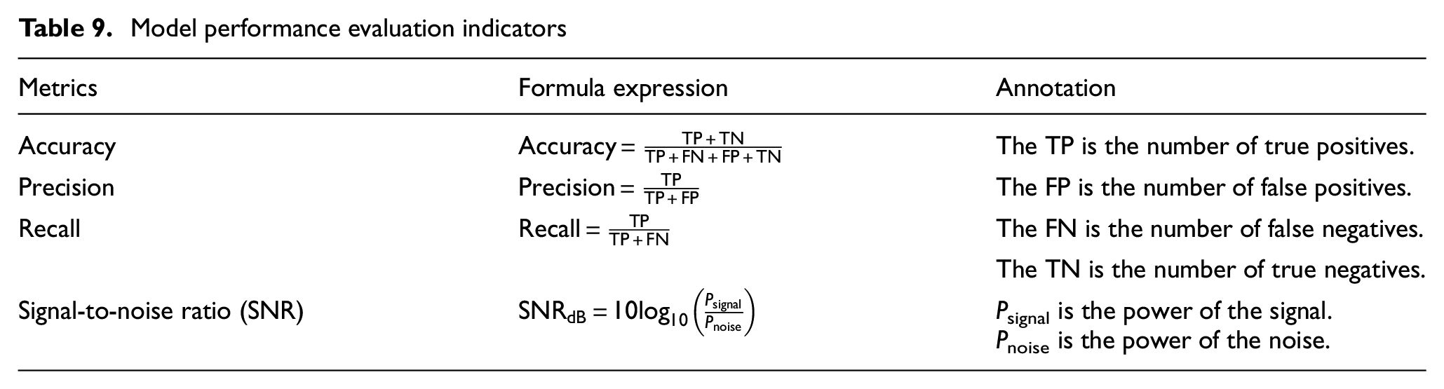
Model performance evaluation indicators
Basic parameter settings
The training setup for the diagnostic model in this paper is as follows: The training and test sets are divided into 8:2. Gaussian white noise is added to the signals to quantify noise intensity. In addition, the network incorporates a Xavier normal distribution initializer and a standard normal distribution initializer for initializing the weights of the convolutional layers and fully connected layers, respectively. Furthermore, we have implemented an early stopping strategy with a threshold of 10 epochs, meaning that when the network converges to a temporary maximum, it still has 10 epochs to converge further. Therefore, the specified number of epochs far exceeds the training convergence requirements, aiming to allow the model to fully converge. The model is trained in cycles, five times each execution, selecting and saving the optimal model. The test set is used to evaluate the actual diagnostic performance of the model. The number of layers in the model is matched to the specific diagnostic task. The training parameters are as follows: The convolutional kernel size and number in the feature filtering layer are 21 × 1 and 16, respectively; the convolutional kernel size and number in the FI layer are 3 × 1 and 8, respectively. The upsampling mode is “linear.” The initial learning rate is set to 0.01, and we have designed a learning rate decay strategy: when the validation accuracy does not improve for three consecutive epochs, the learning rate will be reduced to half of its original value to refine the optimization step size. Batch size is 512. The optimizer used is Adam, the activation function is LuckyReLU, and the loss function is the cross-entropy loss function.
Model parameter selection
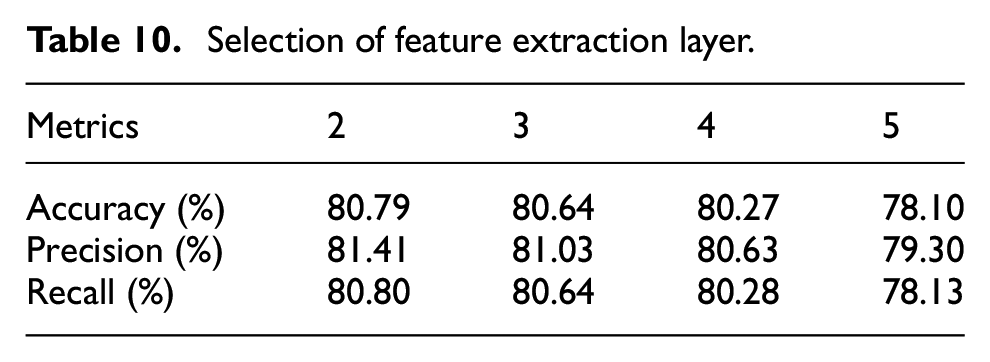
In this paper, the DL-RCD proposed is a versatile model that can be adapted to different data sets by selecting the appropriate structure for the diagnostic task. The experimental data is sourced from the bearing data, at SNR = −4 dB. First, we choose the number of feature extraction layers (a composite block of HWAO and MFEO) for CU. Assuming there are two layers of wavelet decomposition in HWAO and two subsets in MFEO. Due to the disappearance of the JMM module when setting up a composite block, the model lacks complete functionality. Therefore, we abandon this situation. Select feature extraction layers 2, 3, 4, and 5, and the results are shown in Table 10. The results indicate that as the number of extraction layers increases, the performance of the model continues to improve, but the rate of improvement decreases, suggesting that the model’s performance has peaked and further increases in extraction lead to overfitting. Therefore, we chose two layers as the final selection.
Selection of feature extraction layer.
Next, we discuss the impact of wavelet decomposition levels within HWAO on the model. Initially, assuming there are two subsets in MFEO. The model’s feature extraction layer is set to 3. Considering different datasets and device types, the wavelet decomposition level of our proposed universal model needs to be determined according to the following calculation method, with a maximum decomposition level of:
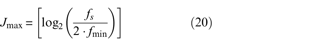
among them, fs is the sampling frequency, and fmin is the lowest effective frequency.
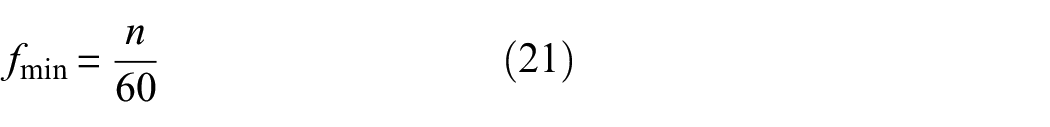
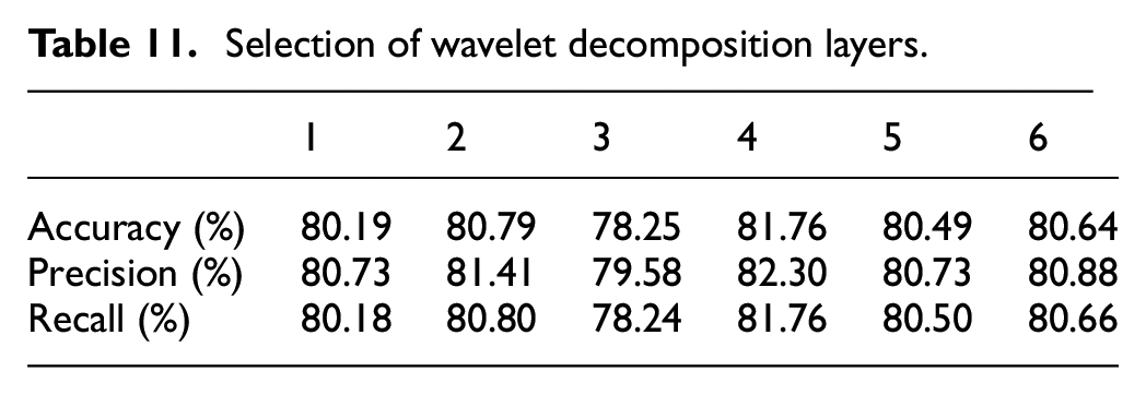
among them, n (rpm) is the rotational speed. In the three different types of datasets mentioned in this article, the lowest effective frequency of the fan is 20 Hz, the lowest effective frequency of the gearbox is 15 Hz, and the lowest effective frequency used for the bearing is 25 Hz. Among them, the sampling frequency of fan data is much smaller than other datasets. As our design is a universal model, it needs to satisfy the minimum decomposition level of data distribution. Therefore, the maximum number of wavelet decomposition layers calculated is 5. To clearly demonstrate the impact of wavelet decomposition level selection on the method’s performance, we conducted experimental validation. The input signal length for the model is 1024, and after initial mapping through the feature filtering layer, the feature map width is 512. We choose to execute a two-layer composite block, so the minimum width of the feature vector is 256. Theoretically, since 2n = 256, n = 8, wavelet decomposition can be performed up to eight times. However, at the eighth and seventh level, only a few data point is included, which loses practical analytical significance. Therefore, we discuss cases where the wavelet decomposition level should be n ≤ 6. The results show that as the number of decomposition levels increases, the performance of the proposed method gradually improves, indicating the effectiveness of our model structure. The experimental results, displayed in Table 11, indicate that a decomposition level of four already meets the model’s needs. However, as the levels continue to increase, performance declines because the frequency resolution of the signal segment improves, but the time resolution decreases. In dynamic fault diagnosis, excessive decomposition can also lead to overfitting noise, boundary effects, and excessive reduction in the resolution of low-frequency components, which hinders the effective capture of rapidly changing fault features, thereby affecting the identification of fault characteristics.
Selection of wavelet decomposition layers.
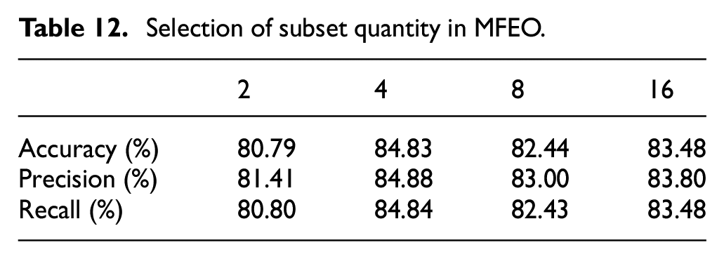
Finally, we determine the number of subsets in MFEO. Since the model is set with 16 channels, the number of subsets should be ≤16. If the number of subsets is 1, there is no multiscale functionality, and it becomes a regular convolution, which does not meet the model’s requirements. Since the number of subsets needs to be divisible by the number of channels, we choose the number of subsets to be a power of 2, namely 2, 4, 8, and 16. The results are displayed in Table 12. From the results, we prefer to choose a subset number of 4, as increasing the number of subsets reduces the interaction of information between channels. If the number of subsets equals the number of channels, it degenerates into a per-channel processing issue. This approach does not mix information between channels and fails to fully capture the correlations among different channels. Facing complex fault patterns in devices, per-channel convolution, due to its fewer parameters, may be limited in expressing complex features. Its performance is more dependent on the quality and quantity of the training data. Per-channel convolution may be more prone to local optima, which could lead to weaker generalization capabilities of the model in practical applications.
Selection of subset quantity in MFEO.
Ablation experiment
A mature diagnostic model typically integrates multiple recognition modalities. The proposed method, DL-RCD, primarily consists of CU, EU, SU, and FU. This allows for the evaluation of each unit’s impact on the model’s diagnostic performance, which is essential for understanding and improving the model. This part of the experiment uses fan data, at SNR = −4 dB, supplemented with white noise. In DL-RCD, removing the dual-path extraction tools in the CU (replaced by 3 × 1 convolution with a stride of 2) is defined as model DL-RCD-I. The absence of the EU in DL-RCD (to ensure operation, the JMM module is replaced by additional operations) is defined as model DL-RCD-II. The absence of the SU is defined as model DL-RCD-III. The absence of the FU (removing SCFM) is defined as model DL-RCD-IV.
First, the five models: DL-RCD, DL-RCD-I, DL-RCD-II, DL-RCD-III, and DL-RCD-IV. The results of these experiments are recorded in Figure 13. The accuracies of DL-RCD, DL-RCD-I, DL-RCD-II, DL-RCD-III, and DL-RCD-IV are 81.91%, 74.67%, 79.11%, 78.01%, and 79.00%, respectively. This indicates that the proposed model can authentically and sufficiently learn sufficient state characteristics that objectively reflect the operation of the equipment. Moreover, DL-RCD-I significantly underperforms compared to DL-RCD-II, DL-RCD-III, and DL-RCD-IV. This is because the lack of functional modules results in the model losing its ability to efficiently converge and capture fault features when faced with the large convergence domain and complex coupling of actual vibration signal representation. DL-RCD-II has an advantage over DL-RCD-III due to its progressive multiscale fusion pattern because DL-RCD-III promptly only emphasizes the expression of detailed information.
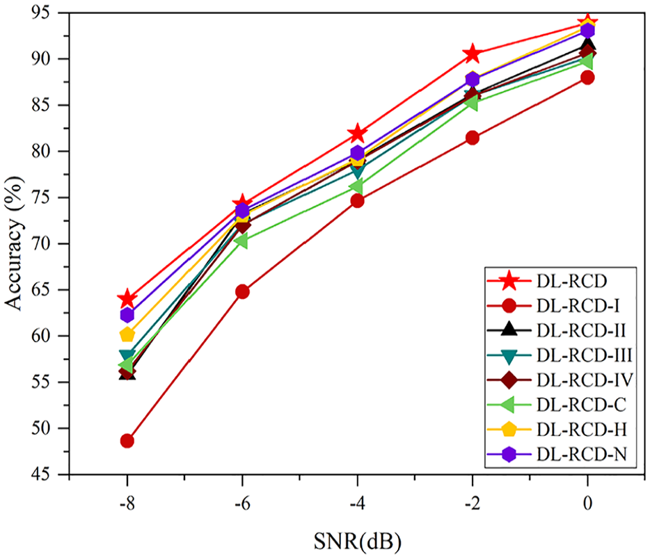
Anti-noise experiment.
In addition, we further discuss the functional performance of the individual units. We remove the HWAO from the CU and designate the model as DL-RCD-C, remove the MFEO module from the CU, and name the model DL-RCD-H. According to the experimental results, DL-RCD-H outperforms DL-RCD-C by 2.97% due to the guidance provided by the wavelet transform, which divides the fault signal into high- and low-frequency intervals, better capturing overall trend characteristics in the low-frequency range and local detail characteristics in the high-frequency range. Furthermore, there are various interpolation methods in the EU. We name the model using the nearest interpolation in the EU as DL-RCD-N. The data shows that the choice of interpolation method has little effect on DL-RCD’s performance, indicating that different interpolation calculations are not highly sensitive to rotor data in the model.
Noise immunity test
In the actual diagnosis of fans, noise interferences such as mechanical, electromagnetic, environmental, resonance, and air vibration are inevitably accompanied. These interferences will enter the model with the data and affect the model’s ability to extract discriminative features. In this part, we construct −8 dB to 0 dB Gaussian white noise interference.
From the experimental results in Figure 13, it can be observed that DL-RCD-I exhibits the largest decline in recognition performance, indicating that the quality of CU in the proposed method plays a crucial role in feature extraction. In addition, DL-RCD-C performs worse than DL-RCD-H, suggesting that the HWAO in the CU is a key tool for effectively coding fault features. As noise increases, the noise resistance advantage of DL-RCD-H becomes more prominent, as the HWAO’s wavelet attention filtering function helps remove outliers and interference, allowing for better capture of fault characteristics across different frequency domains. Although DL-RCD-C can analyze coupling information, it lacks prior theoretical knowledge guidance, resulting in a slightly lower convergence level.
Compared to the CU, the correlation calculation in the SU further aids the model in filtering noise information. This is why DL-RCD-III shows slightly reduced noise resistance compared to DL-RCD. The JMM operation within the SU focuses on specific features related to encoding and decoding, reducing noise interference on the model. Therefore, considering all factors, the proposed DL-RCD model offers greater practical value for wider applications.
Interpretability study
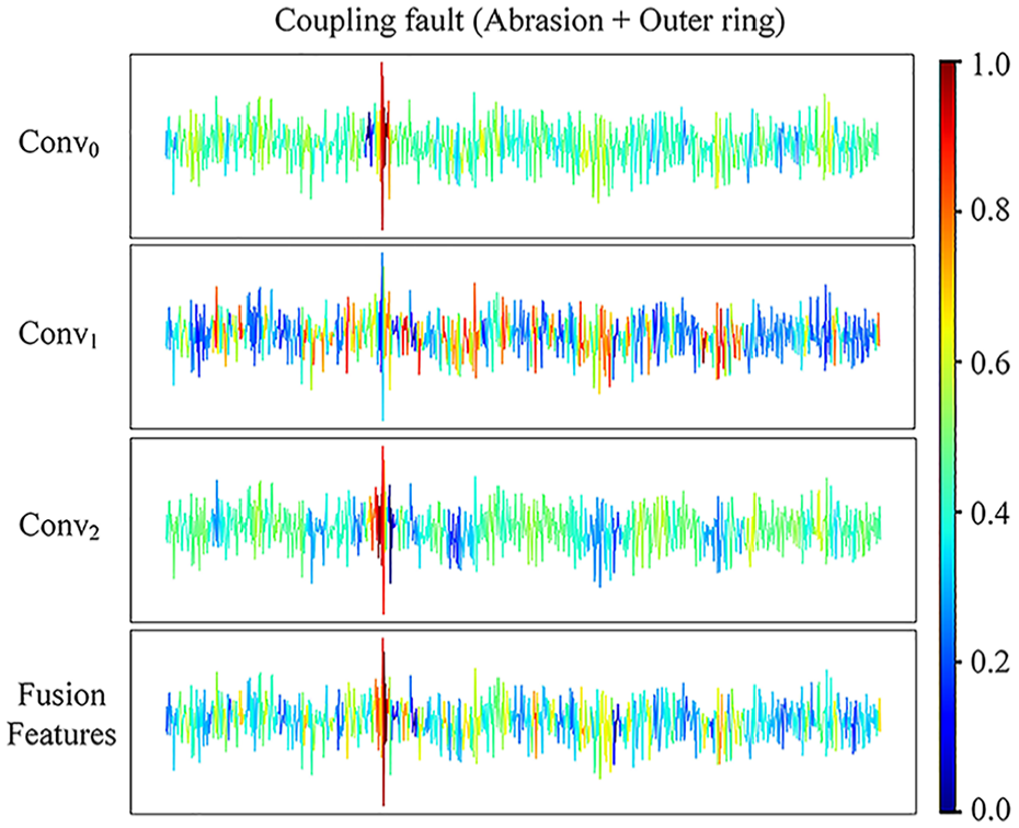
Understanding the importance of features can help decision-makers develop more precise maintenance and operational strategies, reducing downtime and maintenance costs. Gradient weighted class activation mapping (Grad-CAM) generates a thermal distribution map of the input signal by utilizing the gradient information of the model, displaying which regions contribute more to the model’s decision-making and which regions contribute less. Here, we take the time-domain signals of two coupled fault states of a gearbox as an example. Including gear wear—bearing outer ring damage and gear tooth breakage—bearing rolling element damage. The significance distribution of two types of fault signals is shown in Figures 14 and 15.
Visualization results.
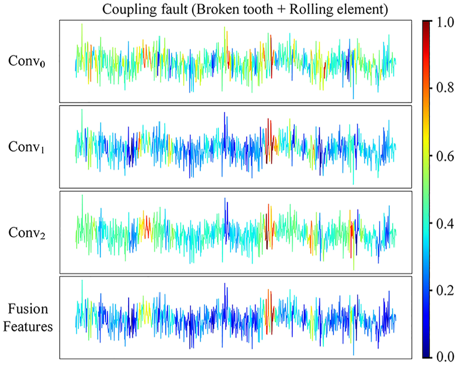
Visualization results.
Conv0 represents the importance of fusion between initial and deep features; Conv1 corresponds to joint discriminant analysis of multiple functional modules; Conv2 corresponds to the fusion expression of deep features and multilevel joint measurements. Finally, fusion features include a comprehensive representation of the discriminative information corresponding to Conv0, Conv1, and Conv2. In Figure 14, a high-frequency transient shock component can be clearly seen. Obviously, the basic extraction function of the model accurately captures this information, which is displayed in the feature maps at Conv0 and Conv2. However, JMM has a certain sensitivity to some discrete small shocks, which may be overlooked by the main extraction function of the model. Considering these subtle discrete discriminative features may improve the model’s learning ability for coupled faults and enhance its utilization of useful information.
The signal distribution in Figure 15 is significantly more chaotic, and slight misalignment is shown in the characteristics of the signal. The main feature learning mechanisms of the proposed model cannot accurately locate the position of discriminative features, and they can only attempt to find some possible discrete impact components. However, the multi-module collaborative measurement mechanism of JMM assigns small weights to possible interference information, while assigning large weights to real discriminative components. Accurately capturing fault signal components from complex pattern signals. The multisource joint analysis strategy of JMM plays a crucial role in improving the learning ability of the model. This influence directly affects the fusion features vector, which in turn greatly impacts the model’s decision-making.
The Grad-CAM visualization method introduced clearly reflects the importance of encoding different information by the model. Accurately explained the inherent functionality of the proposed method, ensuring the stability and trustworthy operation of the model. It is worth noting that our gearbox signal acquisition has a sampling frequency of 10,240 Hz and a minimum speed of 15 Hz. Therefore, a single sample length of 1024 can contain at least one cycle of fault mode. This can also be confirmed by the significance distribution map. The highly activated part expressed in our fusion features graph is only displayed at one position in the signal sample. This fully demonstrates that the model’s behavior of capturing discriminative features is active, accurate in locating useful information, and powerful in locating discriminative signal segments. By identifying which features have the greatest impact on the model’s decision-making, engineers can better understand the behavior of the model. This is crucial for establishing trust and verifying the reliability of the model.
Comparative study
The above experiment effectively verified the reliability of the proposed method. Next, multiple existing excellent models will be compared with the proposed method, and the superiority will be further verified using experimental data from the fan and gearbox. Four SOTA diagnostic models were selected, including LM-MDINet, 28 MA1DCNN, 29 MSCNN, 30 and Wen-CNN. 31 The fan data results are shown in Table 13 and Figure 16.
Comparison results.
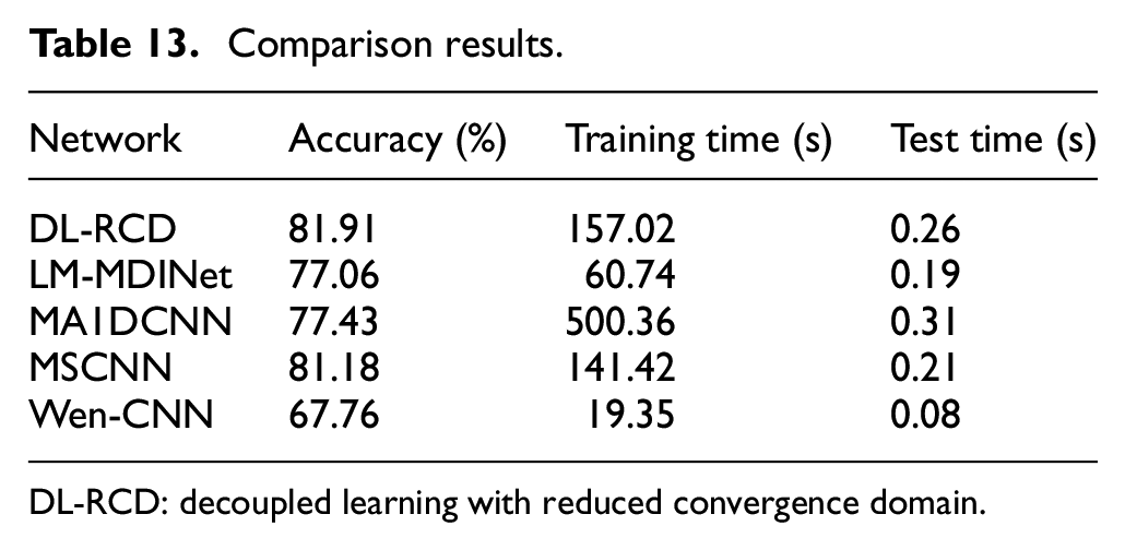
DL-RCD: decoupled learning with reduced convergence domain.
Comparison results of five types of networks on fan data.
Firstly, from the comparison of five models, it is evident that the DL-RCD proposed in this paper has a recognition accuracy of 81.91%, which is approximately 14.15% higher than the lowest-performing model among the other four, Wang et al. 29 have highlighted a significant diagnostic advantage. It is worth mentioning that the diagnosis of these models did not show particularly high levels. This is because in this article, all datasets are standardized using a single sample, resulting in a mismatch between local statistics and global patterns, which is more conducive to training models to deal with sudden failures and high-sensitivity local feature extraction scenarios. In addition, this indicates that the operating conditions of the fan and gearbox are complex, and the signal contains various irrelevant and interfering components, making it somewhat difficult for the model to capture the distribution data pattern. Our study of variable speed and load conditions aligns more closely with real diagnostic needs and better demonstrates the application prospects of the model. Each unit of the model has its own responsibilities, and working together is a meaningful attempt. Second, we identified the three lowest-performing models, Wen et al. 31 converted the data format. Transforming data forms can result in the loss of some information and necessitates adaptation to the model’s extraction mechanism. Lastly, we observed that networks Zhu et al. 28 and Wang et al. 29 also have quite good recognition performance. The primary learning method is through multilayer abstract encoding features. However, when the number of learning layers is insufficient, the model cannot perform at its maximum. The undifferentiated learning strategy requires a larger convergence domain to meet the encoding requirements for complex signals. When too many learning layers are stacked, the model will experience overfitting problems. So, choosing the appropriate number of mappings is a difficult problem. From a macro perspective, diagnostics involve searching for evidence in vibration signals that can indicate a specific fault. However, these proofs may be obscured by interfering factors. Perhaps a singular learning approach cannot adequately observe the differences in these features. This leads to conventional mapping schemes often overlooking unmanifested physical significance and functional features, thereby causing judgment errors.
In terms of training time, there are significant differences among these five models, indicating that the proposed models have certain advantages in both learning ability and resource consumption. In addition, the feasibility of deployment on edge devices such as PLC controllers was reflected through testing time. To avoid missing transient fault signals, real-time fault diagnosis requires a single sample inference delay of less than 50 ms. These models all meet the requirements, but a further balance of efficiency and accuracy is needed.
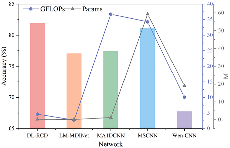
It is worth mentioning that the experimental results of the gearbox data are shown in Figure 17. Compared with Figure 14, the generalization ability of DL-RCD and Zhu et al., 28 Wang et al., 29 and Wen et al. 31 for different datasets does not fluctuate significantly. However, the model in Jiang et al. 30 is more suitable for fan data distribution rather than gearbox data. This is because there are significant differences in the fault signals characteristic of different devices. The feature extraction layer of this model may overadapt to the data characteristics of specific devices, resulting in insufficient cross-device generalization ability.
Comparison results of five types of networks at gearbox data.
Discussion on the trend of industrial equipment health management
The process of industrial equipment intelligence is rapidly reconstructing traditional fault diagnosis systems. This paper proposes a fit multidata mode diagnosis method based on the actual needs of industrial equipment diagnostics, aiming to drive a leap in equipment health management technology through emerging machine learning paradigms. Current technological development is centered around three core directions: the lightweighting of adaptive learning architectures, closed-loop optimization of physics-data collaborative modeling, and a digital twin-driven predictive maintenance framework. The engineering implementation of lightweight adaptive learning systems is crucial for breaking through edge computing scenarios. For example, hyperparameter optimization is based on genetic algorithms and knowledge distillation techniques. The lightweight deployment of models on the edge and asynchronous parameter synchronization can significantly alleviate the problem of industrial data silos 32 . Causal inference-guided physics-data collaborative architecture is a hybrid modeling paradigm born from data sparsity and complex physical mechanisms in industrial scenarios. For instance, the extended Kalman filter generates physical constraints based on vehicle dynamics equations, while the convolutional-bidirectional gated recurrent unit network corrects system errors through spatiotemporal feature fusion, forming a “physics-driven initialization + data-driven correction” closed-loop architecture 33 . Digital twin technology achieves visualization and real-time intervention of equipment degradation mechanisms by constructing a virtual mirror of multi-physics field coupling. For example, time-frequency domain features based on wavelet packet decomposition can be mapped to the virtual twin, dynamically correcting the contact stress distribution model through long short-term memory networks, overcoming the static limitations of traditional threshold monitoring. Twin models achieve cross-condition knowledge transfer through transfer learning, supporting generalized modeling of degradation trajectories for different wear mechanisms, providing a universal framework for predictive maintenance in intelligent manufacturing systems 34 .
The current technological transition has achieved an evolution from a single “perception-cognition-decision” link to an integrated paradigm. In the future, it is necessary to further address issues such as the efficiency of multisource heterogeneous data fusion and the computational power bottleneck at the edge, promoting the development of industrial equipment health management toward full lifecycle intelligence.
Conclusion
This paper presents a novel model, DL-RCD, which analyzes device fault diagnosis issues in practical engineering environments from four perspectives: convergence, coupling, correlation, and efficiency. The work done in this paper includes the following:
The proposed method’s effectiveness was validated using two datasets, one simulating conventional operating conditions and the other simulating complex operating conditions.
The proposed HWAO effectively decouples equipment information under complex conditions while leveraging prior knowledge to enhance the network’s convergence capability. The proposed MFEO combines multiscale mapping, hierarchical fusion, and layered learning to construct a new paradigm of deep encoding for coupled signals at a lower computational cost, which forms the core of CU and enables efficient analysis of signal features under complex conditions.
The network employs a mapping process of encoding–decoding–encoding-interactive output. In SU, the proposed JMM captures the intersection of global and local discriminative information by interacting deep and shallow feature parameters, while SCFM in FU encodes the processed multiscale information in two dimensions, providing a basis for stable final decision-making. This multioperation mapping strategy allows for hierarchical processing of actual operational information, significantly enhancing the model’s diagnostic accuracy, generalization capability, and robustness under real-world conditions.
The proposed DL-RCD method demonstrates the use of different spectrum information of equipment to reduce the convergence domain of the model, thereby lowering computational complexity. The selection of wavelet decomposition levels is based on prior knowledge calculation and experimental validation to achieve optimal results, but automatic optimization has not been implemented. In addition, the DL-RCD incorporates both wavelet decomposition and a self-attention mechanism. While the multifunctional modules in the model can maintain performance while reducing the convergence domain, they may increase additional computation time during offline training, which is not advantageous for dense deployment. Moreover, the application of the self-attention mechanism is undoubtedly not the lowest complexity choice. This additional computational complexity may further increase storage requirements in hardware deployment.
In future research, it is important to enhance the guidance of signal processing priors within deep learning models, improving the level of automatic optimization to reduce the likelihood of selecting suboptimal features and ensuring generalization across small and diverse datasets. This approach can facilitate deployment on low-computation-power terminals and help address issues related to data distribution shifts. Furthermore, consideration should be given to constructing a frequency band relationship graph, where nodes represent specific frequency band energy values and edges represent energy transfer relationships between bands. Within this graph, defining fault propagation paths (e.g., bearing wear → low-frequency harmonic enhancement → high-frequency impact occurrence) and utilizing unsupervised walk strategies can capture potential fault evolution patterns.
Footnotes
Author contributions
Declaration of conflicting interests
The author(s) declared no potential conflicts of interest with respect to the research, authorship, and/or publication of this article.
Funding
The author(s) disclosed receipt of the following financial support for the research, authorship, and/or publication of this article: This study was supported by Fundamental Research Funds for the Central Universities (grant number: 2019MS094).
Data availability
The datasets generated or analyzed in the process of this paper can be obtained from the corresponding author upon reasonable request for a report of the current study.