Rolling bearings fault diagnosis under various loads conditions based on GWJO-VMD-MAFCNN

Abstract

In response to the unclear fault characterization of rolling bearing vibration signals due to their nonlinear and nonstationary characteristics, a rolling bearing fault diagnosis method based on grey wolf jackal optimization algorithm variant mode decomposition multi-activation function convolutional neural networks (GWJO-VMD-MAFCNNs) is proposed. The multi-activation function convolutional networks (MAFCNNs) utilize both Tanh and Softmax activation functions to achieve better diagnostic results. Meanwhile, we leverage the GWJO to optimize the parameters σ and K of VMD, employing the refined VMD for fault diagnosis of the original bearing signals. Subsequently, the permutation entropy of the multiple intrinsic mode function components decomposed by VMD is used as a sample, which is then input into the MAFCNN for training. The experimental results show that the GWJO-VMD-MAFCNN achieved a 100% accuracy rate in all five trials, demonstrating the best diagnostic performance. Additionally, the proposed MAFCNN had the smallest validation loss, with the GWJO-VMD-MAFCNN reaching a validation loss of 2.13e⁻⁶, indicating that the proposed method has a high degree of accuracy. The comparative test data demonstrates that the performance of the GWJO-VMD-MAFCNN is superior to the existing optimization techniques.

Keywords

Rolling bearings fault diagnosis VMD grey wolf jackal optimization multi-activation function convolutional neural networks

Introduction

At present, there exist several limitations in the realm of diagnosing, analyzing, and predicting rolling bearing faults both domestically and internationally. For instance, certain research indicates that the accuracy of bearing fault diagnosis can vary under diverse operating conditions, or the model may exhibit a lack of robustness in generalizing to novel situations or previously unseen faults. This often necessitates an expanded collection of samples and data for further verification and refinement of the models. In response to this situation, this article proposes a new rolling bearing fault diagnosis algorithm called grey wolf jackal optimization algorithm variant mode decomposition multi-activation function convolutional networks (GWJO-VMD-MAFCNN). The main contributions are the introduction of a novel grey wolf jackal optimization (GWJO) and multi-activation function convolutional networks (MAFCNN), and a fault diagnosis method that integrates variant mode decomposition (VMD) decomposition technology and permutation entropy feature extraction technology. This method, with its strong signal analysis and processing capabilities and strong model generalization ability, provides new ideas and solutions for the health monitoring and fault diagnosis of rolling bearings.

Rolling bearing is a kind of precision mechanical component, which is widely used in the fields of automobile, electric power equipment, rotating machinery, mining equipment, and marine equipment.^1,2 Rolling bearings in the working state often face a variety of complex rotating loads.^3,4 When rolling bearings are running at high speed, due to the high contact stress between the rolling element and the inner and outer rings, the bearing life may be reduced, and even fatigue damage may occur, thus causing serious consequences to the production process.⁵ If the rolling bearing is not diagnosed and maintained in time, it may lead to equipment shutdown, production damage, and personnel injury, resulting in serious economic and personal safety risks.⁶ Hence, the timely diagnosis of faults in rolling bearings is of paramount importance.

Vibration signals of rolling bearings have nonlinear characteristics such as nonstationary, impact, multifractal, etc. In addition, they are also affected by many factors, so it is extremely important to extract the effective information from them.⁷ Traditional nonlinear signal analysis includes time-domain and frequency-domain methods. In the time domain, statistical parameters and autocorrelation functions are used to describe the characteristics, while in the frequency domain, the frequency components are studied by the Fourier transform. The time–frequency analysis method proposed based on traditional analysis methods has the advantage of simultaneously displaying the characteristics of time domain and frequency domain when analyzing signals and can accurately locate the time-varying frequency components of signals, flexibly adapt to different processing requirements, and is widely used in many fields.⁸ The most commonly employed time–frequency analysis techniques predominantly consist of the short-time Fourier transform (STFT), continuous wavelet transform, and empirical mode decomposition (EMD).^9–11 The essence of the EMD algorithm lies in its ability to decompose the original signal into several intrinsic mode functions (IMFs). Each of these IMF components captures a distinct local characteristic of the signal, enabling the representation of various frequency components within it. This approach facilitates both time–frequency analysis and the de-noising of intricate signals. Many experiments have shown that the EMD method has a significant effect on signal decomposition and the removal of internal noise.¹² However, due to the discontinuity and mutation characteristics of signal endpoints as well as the complexity and noise interference of signals, EMD method is prone to the phenomenon of end-effect and mode overlap, which will seriously affect the accuracy and reliability of EMD decomposition results and reduce the effectiveness and credibility of the entire analysis process.¹³ In 2014, Dragomiretskiy and Zosso¹⁴ introduced a groundbreaking signal-processing method known as variable mode decomposition (VMD). This method adeptly converts the issue of signal decomposition into a challenge of constrained optimization. It addresses the long-standing issues of end-effects and mode mixing that have baffled researchers by utilizing variational models. In addition, the VMD method also has excellent decomposition performance and realizes efficient signal processing. Li et al.¹⁵ combined VMD and nonlinear wavelet threshold technology to successfully de-noise signals containing a large amount of environmental noise through experiments, further verifying the feasibility of VMD method. In 2022, Zhou et al.¹⁶ suggested a diagnostic model for identifying faults in rolling bearings, in which VMD method was used in feature extraction to decompose vibration signals during bearing operation to obtain the effective information.

As machine learning and deep learning technologies continue to evolve, the integration of sophisticated learning algorithms with the identification of rolling bearing faults has garnered significant interest in both academic and industrial circles. The most used algorithms are random forest, support vector machine (SVM) commonly, graph neural networks (GNNs), and convolutional neural networks (CNNs). Wu et al.¹⁷ cleverly made use of the machine learning algorithm random forest to successfully conduct accurate and efficient fault diagnosis for industrial robots in the working process. This approach not only enhances the precision of fault detection but also significantly cuts down on the time required for diagnosis. Wang et al.¹⁸ innovatively adopted SVM as a fault diagnosis model and successfully realized accurate bearing fault diagnosis through in-depth analysis and processing of rolling bearing vibration signals, temperature data, and other relevant parameters. Yu et al.¹⁹ recently proposed an innovative fault diagnosis framework, which combines GNN and dynamic graph embedding (DGE). They deeply explored the advantages of GNN in dealing with complex system structures and skillfully introduced DGE into the framework to achieve accurate capture of system dynamic characteristics. To achieve the accurate fault diagnosis of rolling bearings, Zhao et al.²⁰ proposed an innovative method of fractal feature extraction based on CNN and principal component analysis (PCA), which combined deep learning technology and traditional signal-processing technology to effectively solve a series of challenges in rolling bearing fault diagnosis.

Although VMD has made some progress in solving problems such as endpoint effects and modal confusion, it is still a challenging task to accurately select decomposition layers and adjust secondary penalty factors. CNN has not only achieved great success in the field of deep learning but also has some drawbacks. The CNN requires extensive and varied datasets for training. Insufficient or imbalanced training data can result in the issue of overfitting. When CNN processes one-dimensional signals, the convolution operation of CNN may not be able to capture key features adequately because one-dimensional signals often have more complex and variable structures. This can cause the model to have difficulty in recognizing and understanding one-dimensional signals. Moreover, due to the characteristics of a one-dimensional signal, CNN may need a deeper network level and more parameters when processing. This not only increases the complexity of the model but also may lead to a decrease in computational efficiency.

In this study, the rolling bearing’s vibration signal is initially decomposed using the VMD technique. Then, we introduce a new optimization algorithm based on grey wolf optimization (GWO) and golden jackal optimization (GJO), GWJO algorithm. The algorithm is used to optimize the optimal quadratic penalty factor and the number of decomposition layers in VMD to determine the best decomposition result, after obtaining the optimal values of these two parameters, they are then returned to VMD. After the signal is decomposed, the eigenvector is constructed by means of permutation entropy and other methods. Then, we utilize the MAFCNN as our diagnostic model. By inputting the extracted feature vectors and training the model, the MAFCNN is capable of autonomously learning to recognize the distinctive characteristics of various fault patterns, thereby achieving precise fault mode identification. Ultimately, the MAFCNN model’s output results are assessed using test samples. The fault diagnosis methodology is subsequently subjected to a comprehensive assessment, focusing on aspects such as time–frequency signal characteristics, the optimization fitness curve, and the fault diagnosis accuracy. This evaluation aims to substantiate its efficacy and precision in identifying faults in rolling bearings.

Study of the GWJO algorithm

VMD method

VMD is a flexible and entirely iterative signal-processing technique that operates on the foundation of modal variational analysis. One of the key benefits of this method is its capacity to autonomously ascertain the requisite number of modal components for signal decomposition. During the decomposition process, VMD can automatically adjust the optimal central frequency and bandwidth constraints for each mode to accommodate the actual characteristics of the signal. This method effectively separates the IMF within the signal and performs frequency-domain analysis, thereby achieving an effective decomposition of the signal. Ultimately, it addresses the variational challenge and secures the most favorable outcome.

Supposing that the original signal F is split into k constituent parts, the goal is to ensure that these decomposition parts are modal components characterized by central frequencies and limited bandwidths, and to achieve this while minimizing the total estimated bandwidth of each modal component. The condition is that the aggregate of all these components must reconstruct the original signal. The formulation of the VMD constrained variational model can be expressed as follows:

min_{{u_{k}, w_{k}}} {\sum_{k} {‖ \partial_{t} [(δ (t) + \frac{j}{\bar{x} t}) \times u_{k} (t)] \exp (- j ω_{k} t) ‖}_{2}^{2}}

(1)

s . t . \sum_{k} u_{k} = F

(2)

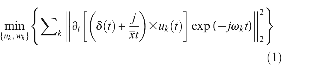
where ω_k is the frequency center of each IMF; u_k is the k-th IMF; f is the original signal.

To address the aforementioned constrained optimization challenge, the problem is reformulated from a constrained to an unconstrained form. Utilizing the benefits of a quadratic penalty function along with the technique of Lagrange multipliers, an enhanced Lagrange function is devised, which is depicted in the following equation:

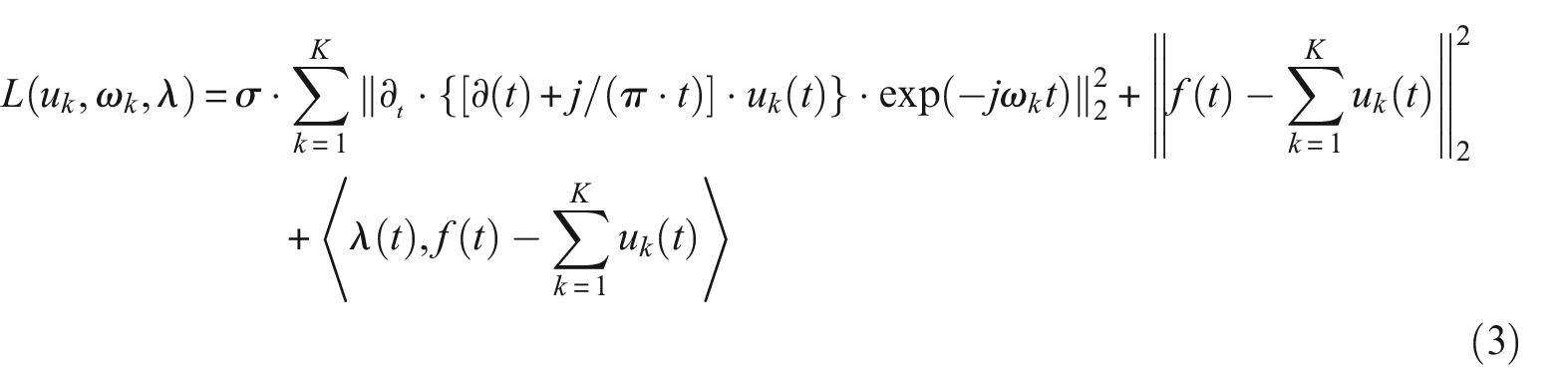
\begin{matrix} L (u_{k}, ω_{k}, λ) = σ \cdot \sum_{k = 1}^{K} {‖ \partial_{t} \cdot {[\partial (t) + j / (π \cdot t)] \cdot u_{k} (t)} \cdot \exp (- j ω_{k} t) ‖}_{2}^{2} + ‖ f (t) - \sum_{k = 1}^{K} u_{k} (t) ‖_{2}^{2} \\ + 〈 λ (t), f (t) - \sum_{k = 1}^{K} u_{k} (t) 〉 \end{matrix}

(3)

where σ is the penalty factor; $λ$ is the Lagrangian multiplier.

The technique of employing the alternating direction method of multipliers is utilized to locate the saddle point of the variational problem. This approach enables the iterative refinement of the central frequency and bandwidth for each IMF signal.

ω_{k}^{n + 1} = \frac{\int_{0}^{\infty} ω \cdot {| {\hat{u}}_{k} (ω) |}^{2} d ω}{{\int_{0}^{\infty} | {\hat{u}}_{k} (ω) |}^{2} d ω}

(4)

{\hat{u}}_{k}^{n + 1} (ω) = \frac{\hat{f} (ω) - \sum_{i \neq k} {\hat{u}}_{i} (ω) + \hat{λ} (ω) / 2}{1 + 2 \cdot σ \cdot {(ω - ω_{k})}^{2}}

(5)

\hat{f} (ω) - \sum_{i \neq k} {\hat{u}}_{i} (ω)

(6)

where ${\hat{u}}_{k}^{n + 1} (ω)$ is the filtering result of residual quantity in equation (6); $ω_{k}^{n + 1}$ is the power spectrum center of gravity of the current mode; and the real part can be obtained by inverse fast Fourier transformation of ${\hat{u}}_{k} (t)$ .

The decomposition steps of VMD are as follows (Figure 1):

Step1: Initialize parameter u_k, ω_k, λ, σ, and n = 0, k = 0;

Step2: Increment the iteration count by one, denoted as n = n + 1, and proceed with the VMD algorithm for the next cycle of iterative computation;

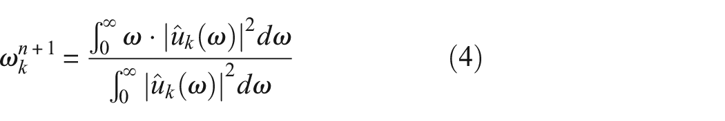
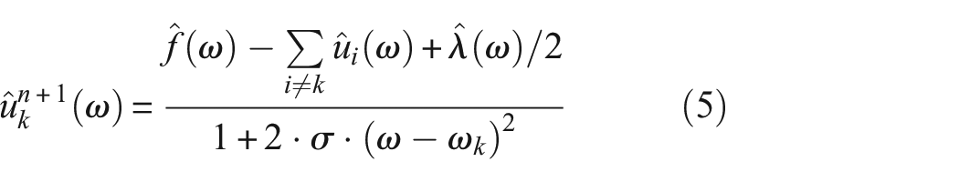
Step3: Increment the index by one, signified as k = k + 1, and update the variables u_k and ω_k in accordance with the equations (3) and (4);

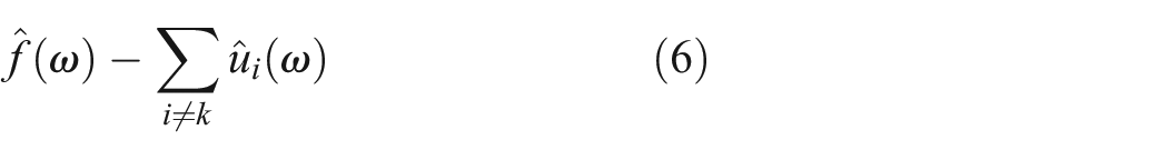
Step4: Adjust the value of λ based on the subsequent formula provided:

λ^{n + 1} = λ^{n} + τ \cdot (f - \sum_{k} {\hat{u}}_{k}^{n + 1})

(7)

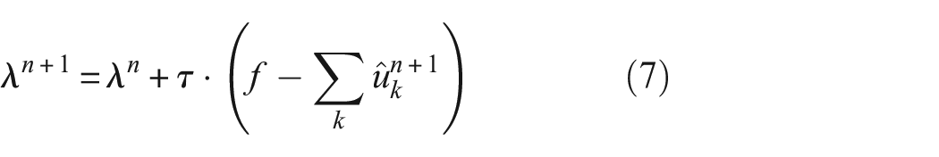
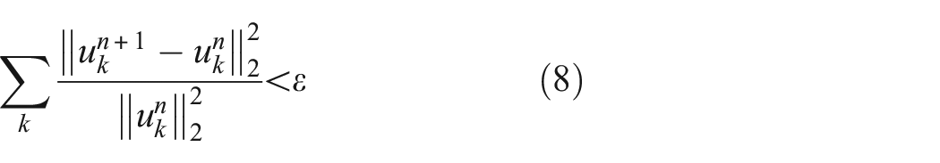
Step5: Specify a judgmental precision threshold ε > 0 and continue the process until the following termination condition is satisfied:

\sum_{k} \frac{‖ u_{k}^{n + 1} - u_{k}^{n} ‖_{2}^{2}}{‖ u_{k}^{n} ‖_{2}^{2}} < ε

(8)

Figure 1.

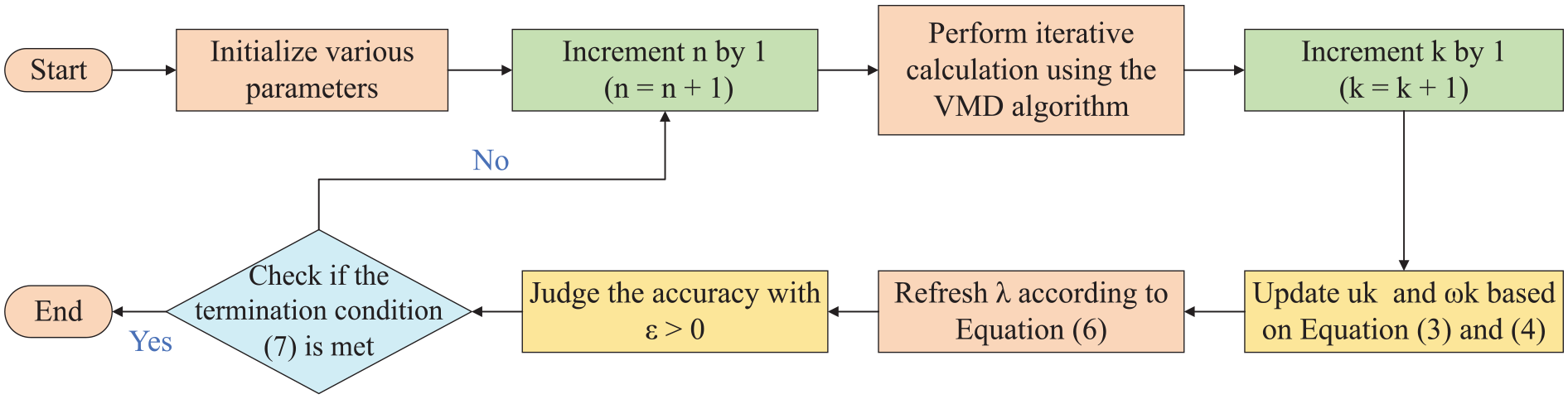
The working principle of VMD.

VMD overcomes the issues of endpoint effects and modal component aliasing and is founded on a more robust mathematical theory. It can reduce the nonstationarity of time series with high complexity and strong nonlinearity, decomposing them into subsequences that contain multiple different frequency scales and are relatively stable. This makes it suitable for nonstationary sequences and easier to identify and analyze potential fault characteristics, thereby improving the accuracy and efficiency of fault detection.

The proposed GWJO algorithm

The principle of GWO

GWO is an algorithm proposed by Mirjalili et al.²¹ The wolf population consists of various roles, including the α wolf, β wolf, δ wolf, and ω wolf.²² In GWO, the search operations are directed by the top three wolves, designated as α, β, and δ. These leaders share equal influence in the updating formula, with each holding a one-third weight.²³ Grey wolf ω accepts grey wolves during the hunting of α, β, and δ.¹⁶ The progression of the grey wolf algorithm can be segmented into three principal phases: encirclement, pursuit, and attack.^24,25 The detailed steps are outlined below:

Step1: Encircle the prey.

When grey wolves hunt, they strategically move closer and surround their prey. The mathematical representation of this hunting strategy is as follows:

D = | C \cdot x_{p (t)} - x_{t} |

(9)

x_{t + 1} = x_{p (t)} - A \cdot D

(10)

A = 2 \cdot a \cdot r_{1} - a

(11)

C = 2 \cdot r_{2}

(12)

where t indicates the current iteration; D represents the distance between the grey wolf individual and its prey, while A and C are vectors of the cooperation coefficients; x_p denotes the position vector of the prey; x_t indicates the current position vector of the grey wolf. Throughout the iterative process, a linearly decreases from 2 to 0; r₁ and r₂ are random vectors within the range [0, 1].

Step2: Hunting.

Grey wolves are adept at pinpointing the location of their prey, with hunts typically spearheaded by the α, occasionally joined by the β and δ wolves. Nevertheless, in many cases, the properties of the solution space are obscure, which hinders grey wolves from pinpointing the exact location of their quarry. To emulate the hunting tactics of grey wolves, we presume that the α, β, and δ wolves are equipped to detect probable locations where the prey might be. Consequently, in each iteration, the top three performing grey wolves are selected based on their performance, and subsequently, the positions of the remaining search agents are adjusted according to the positional data of these top wolves. Therefore, the following formula is proposed:

D_{α} = | C_{1} \cdot x_{α} - x |, D_{β} = | C_{2} \cdot x_{β} - x |, D_{δ} = | C_{3} \cdot x_{δ} - x |

(13)

x_{1} = x_{α} - A_{1} \cdot D_{α}, x_{2} = x_{β} - A_{2} \cdot D_{β}, x_{3} = x_{δ} - A_{3} \cdot D_{δ}

(14)

x (t + 1) = \frac{x_{1} + x_{2} + x_{3}}{3}

(15)

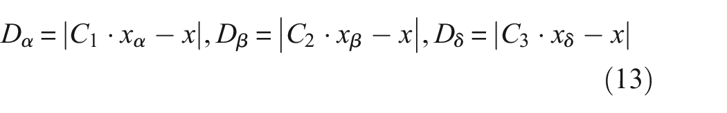
In this description, x_α, x_β, and x_δ are the position vectors corresponding to the α, β, and δ wolves within the current population, respectively. The term x refers to the position vector of a particular grey wolf. Additionally, D_α, D_β, and D_δ are the measures of the distances from the current grey wolf candidates to the top three wolves that are leading in performance. When (|A| > 1), grey wolves are dispersed across various regions and search for prey. When (|A| < 1), grey wolves will concentrate on searching for prey in one or several areas.

Figure 2 illustrates the process by which the search agent adjusts its position within a two-dimensional search space based on the values of α, β, and δ. Data gathered from observations suggest that the ultimate location of an agent is likely to be randomly distributed within a circular region, the boundaries of which are determined by the positions of the α, β, and δ wolves in the search space. To put it on another way, the α, β, and δ wolves are employed to gauge an approximate area where the prey might be located, and based on this approximation, the other wolves adjust their positions in a random manner around the estimated location of the prey. Figure 2 also presents the wolf pack’s social hierarchy using a pyramid structure. The social structure of the wolf pack is divided into four levels: At the top is the α wolf, which is responsible for making decisions on hunting, habitat, and daily activities. The α wolf is not necessarily the strongest, but it is the most outstanding in leadership ability. The second level is the β wolf, which assists the α wolf in decision-making and takes over its position when the α wolf is absent and can also command other wolves. The third level is the δ wolf, which obeys the α and β wolves but can control wolves at other levels, usually composed of wolves with different roles. At the bottom is the ω wolf, which, although it has the lowest status, is crucial for maintaining the harmony of the pack and preventing internal conflicts.

Step3: Attacking prey.

Figure 2.

The position update and hierarchical system of the wolf pack in the GWO algorithm.

From equation (11) in Step 1, it can be seen that the value of A fluctuates with changes in the value of a. To mathematically model the approach and attack on the prey, the value of a is decreased, it means that A is within a random interval of [−a, a]. In other words, if A falls within the range of [−1, 1], the search agent’s position at the subsequent moment may be situated at any point along the line connecting the current grey wolf and its prey, signifying an ongoing predatory assault. Conversely, if the absolute value of A exceeds 1, it implies that the wolf is unable to commence an attack on its prey. As shown in Figure 3, it illustrates the impact of parameter A on the wolf pack’s attack on prey.

Figure 3.

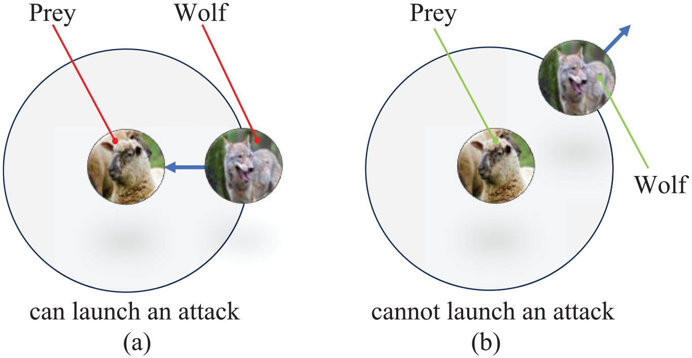
The model of attacking prey (a) |A| < 1 and (b) |A| > 1.

The GWO algorithm is inherently non-greedy, possessing good global optimization capabilities, thus making it less likely to fall into local optima. In GWO, the value of the convergence factor A typically decreases linearly from a larger value to 0. This linear decrement strategy may not be the most effective, as it does not adapt well to the search requirements at different stages, which may lead to an improper balance between local search and global exploration, thereby affecting the convergence speed.

The principle of GJO

The GJO is an innovative optimization technique, drawing its inspiration from the collaborative hunting strategies employed by golden jackals.²⁶ The fundamental concept of this algorithm involves associating the positions of the golden jackals with potential solutions within the algorithm’s search domain, and it regards the gap between each jackal and its target as a measure of the solution’s fitness.²⁷ The jackal irritates the prey, causing its will to flee to diminish. As a result, the prey becomes trapped by the two jackals. With the prey confined, the pair of jackals then launch an assault and consume the prey.²⁸ But during the searching phase, the algorithm may fall into local optimal solutions due to the lack of diversity in the search strategy or the limitations of the updating mechanism, especially when solving complex or high-dimensional optimization problems. The formula of GJO in exploration stage is as follows:

x_{1} (t) = x_{M} (t) - E . | x_{M} (t) - rl . Prey (t) |

(16)

x_{2} (t) = x_{FM} (t) - E . | x_{FM} (t) - rl . Prey (t) |

(17)

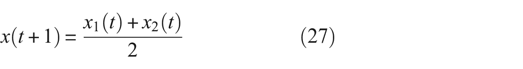
where t indicates the current iteration, Prey(t) is the position vector of the prey, x_M(t) and x_FM(t) represent the positions of the male and female jackals, respectively. x₁(t) and x₂(t) are the updated positions of the male and female jackals corresponding to the prey.

E represents the prey’s evasion energy, and it is calculated using the following formula:

E = E_{1} \times E_{0}

(18)

where E₁ represents the decreasing rate of the prey’s energy, while E₀ denotes the initial state of the prey’s energy,

E_{0} = 2 \times r - 1

(19)

where r is a random number between 0 and 1.

E_{1} = c_{1} \times (1 - (t / T))

(20)

T refers to the upper limit of the iteration count, with c₁ being a constant set at 1.5, and t representing the iteration number currently in progress. E₁ is progressively reduced linearly from an initial value of 1.5 down to 0 across the entire span of iterations.²⁹

The multiplication of rl and Prey simulates the movement of the prey in a Lévy flight manner, with the calculation formula as follows³⁰:

rl = 0.05 \times LF (y)

(21)

LF (y) = 0.01 \times (μ \times σ) / (| ν^{(1 / β)} |)

(22)

σ = {(\frac{Γ (1 + β) \times \sin (π β / 2)}{Γ ((1 + β) / 2) \times β \times (2^{(β - 1) / 2})})}^{1 / β}

(23)

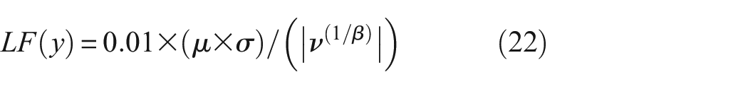
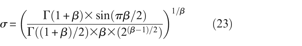
where u and v are random values within the interval [0, 1], β is a constant with a value of 1.5.

x (t + 1) = \frac{x_{1} (t) + x_{2} (t)}{2}

(24)

The principle of GWJO

Due to the good global optimization capability of GWO, its convergence speed is relatively slow; the global optimization ability of GJO is not as strong as GWO; however, the convergence speed of GJO is faster than GWO; in GWO, the primary mechanism by which grey wolves locate their prey is through the use of the α, β, and δ parameters. Initially, the search for prey locations is conducted in a dispersed fashion, which then transitions into a focused attack. A crucial component of the GWO algorithm is the search coefficient, denoted as C. As depicted in equation (12), the C vector is comprised of random numbers that fall within the interval [0, 2]. This coefficient assigns variable weights to the prey, either amplifying (when the absolute value of C is greater than 1) or attenuating (when it is less than 1) the search intensity. This mechanism fosters a stochastic search behavior, which is instrumental in preventing the algorithm from becoming trapped in local optima. It is important to recognize that C does not diminish in a linear fashion; rather, it fluctuates randomly throughout the iterations. This randomness of C is especially significant in the later iterations, aiding the algorithm in escaping from local optima.

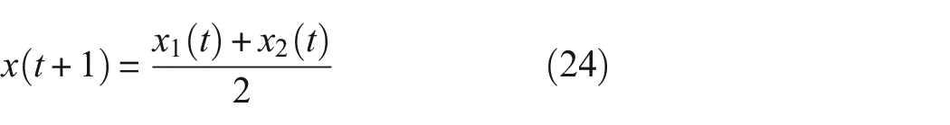
Although the GJO algorithm utilizes randomness to simulate the hunting behavior of golden jackals, the introduction of randomness may also lead the algorithm to encounter local optimal solutions and become stuck there during the search process, especially during the searching phase. Inspired by the above, we introduce the search coefficient C into the GJO algorithm to avoid falling into local optima, the GWJO algorithm is proposed. The equations of the exploration stage are as follows:

x_{1} = x_{M} (t) - E . | x_{M} (t) - C \cdot Prey (t) |

(25)

x_{2} (t) = x_{FM} (t) - E . | x_{FM} (t) - C \cdot Prey (t) |

(26)

x (t + 1) = \frac{x_{1} (t) + x_{2} (t)}{2}

(27)

where x₁(t) and x₂(t) indicate the position of male and female jackals, respectively, in the GWJO; x(t+1) denotes the updated position of the jackals.

Equations (25)–(27) show that the GWJO algorithm is based on the main structure of the GJO, the fast convergence speed of the GJO algorithm is retained, and at the same time, the search parameter C is introduced into the improved GJO, making the GWJO algorithm less likely to fall into local optima. Based on the theoretical foundation of the GWO and GJO algorithms, and by introducing the parameter C, the GWJO algorithm integrates the advantages of both. The specific working principle is shown in Figure 4.

Figure 4.

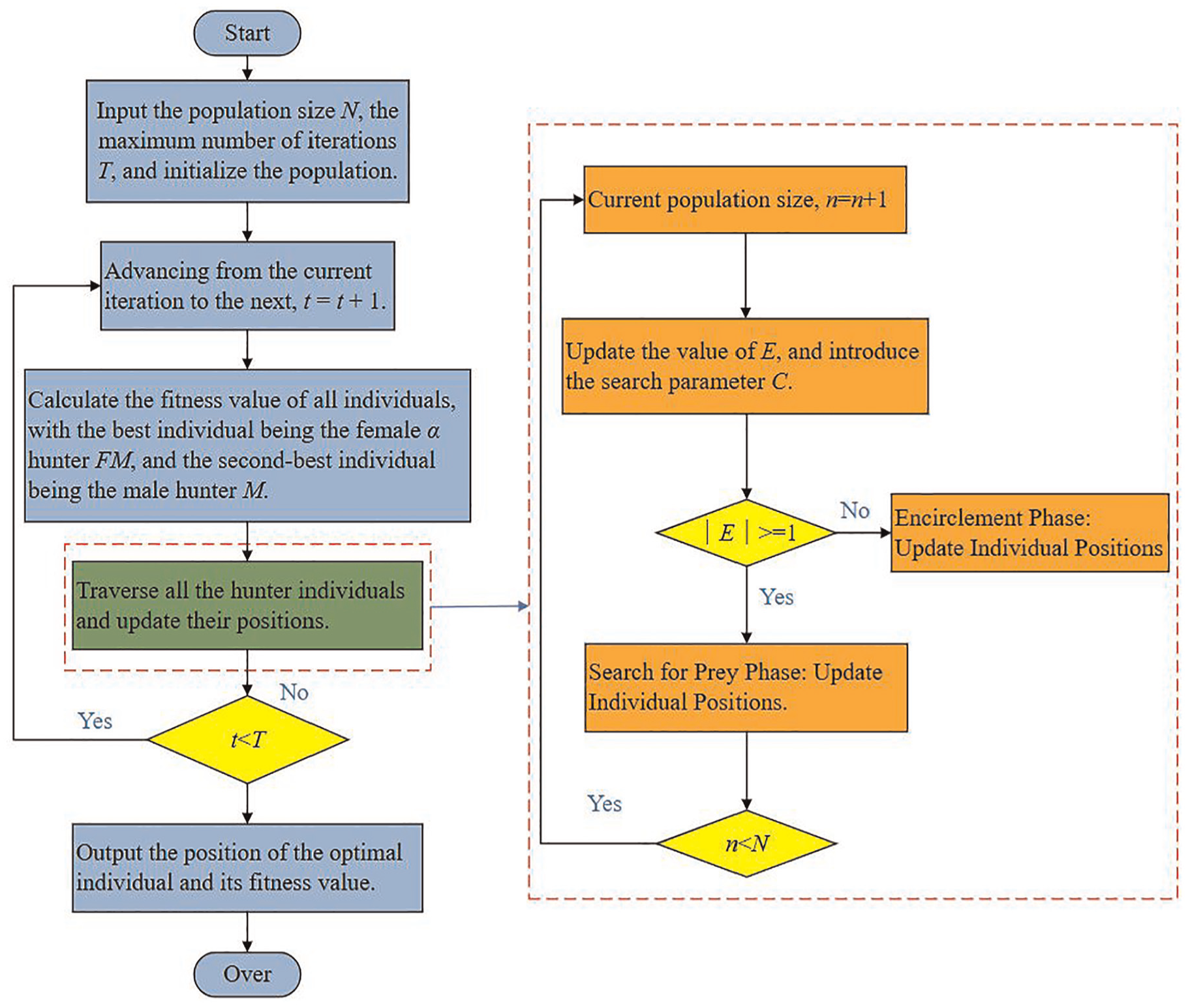
The process principle of GWJO.

As delineated in Figure 4, the GWJO algorithm innovates by integrating a search parameter C during the hunters’ position updates. This inclusion significantly influences the exploration phase, augmenting the algorithm’s capacity for global optimization. The parameter C serves as a catalyst for a more comprehensive search, ensuring a broader exploration of the solution space and thus increasing the likelihood of identifying the most optimal solution. This strategic enhancement positions the GWJO algorithm as a powerful tool for complex optimization tasks, particularly in scenarios demanding high accuracy and efficiency, especially in the optimization of VMD parameters for advanced signal processing and feature extraction in fault diagnosis applications.

VMD optimized based on the GWJO algorithm

In the domain of signal processing, VMD is adept at managing signals effectively. It operates by iteratively seeking out the optimal solution for a variational model, which allows for the identification of the intrinsic properties of each constituent signal component. This approach is characterized by a completely non-iterative model. However, when using VMD, there are two important parameters. The first one is the number of modes, K. When the value of K falls short of the count of beneficial components within the signal destined for decomposition, it precipitates an under-decomposition scenario, which in turn induces modal aliasing and a decomposition that is not fully realized. On the flip side, if K exceeds the tally of beneficial components, it incites an over-decomposition condition, fabricating a set of redundant and ineffectual components.

The second important parameter is the penalty factor σ, which plays a crucial role in the quality of signal decomposition in VMD. An appropriate value can help the algorithm more accurately extract physically meaningful modes from complex signals, while an inappropriate value may lead to mode aliasing or distortion in the results. The determination of these two values largely depends on trying various ranges, which has limited applicability.¹⁴

Hence, enhancements to the VMD algorithm are necessary to facilitate the easier selection of the appropriate number of decomposition layer number K and penalty factor σ, to ensure the accurate signal decomposition of rolling bearing vibrations. In this study, the GWJO algorithm is employed to refine the algorithm’s parameters and dynamically identify the optimal parameter set.

Permutation entropy serves as a technique for identifying randomness and sudden dynamic changes within time series data, making it extensively utilized for condition monitoring, fault diagnosis, and assessment of signals across various mechanical systems. Given the unique attributes of permutation entropy, the permutation entropy values of the individual components derived from VMD are harnessed as the fitness criteria for optimizing the GWJO algorithm.

Assuming there is a signal of length N {X(i), i = 1, 2, …N}, the calculation method for permutation entropy is as follows³¹:

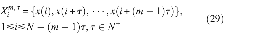
Step 1: Sequence segmentation: Given an embedding dimension of m and a sampling rate of τ, generate a sequence of vectors.

X_{1}^{m, τ}, . . ., X_{N - (m - 1) τ}^{m, τ}

(28)

\begin{matrix} X_{i}^{m, τ} = {x (i), x (i + τ), \dots, x (i + (m - 1) τ)}, \\ 1 \leq i \leq N - (m - 1) τ, τ \in N^{+} \end{matrix}

(29)

Step 2: Sequence sorting: Sort the elements within the X sequence to obtain the sorted indices.

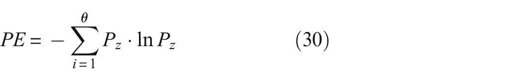
Step 3: Within an m-dimensional phase space, there exist a total of m! distinct possible sequences of symbols, with X being just one among these various sequences. If we denote the occurrence probabilities of these sequences as P₁, P₂, …, P_n, then the permutation entropy is determined using the following formula:

PE = - \sum_{i = 1}^{θ} P_{z} \cdot \ln P_{z}

(30)

The VMD optimization process utilizing the GWJO algorithm is depicted in Figure 5:

Figure 5.

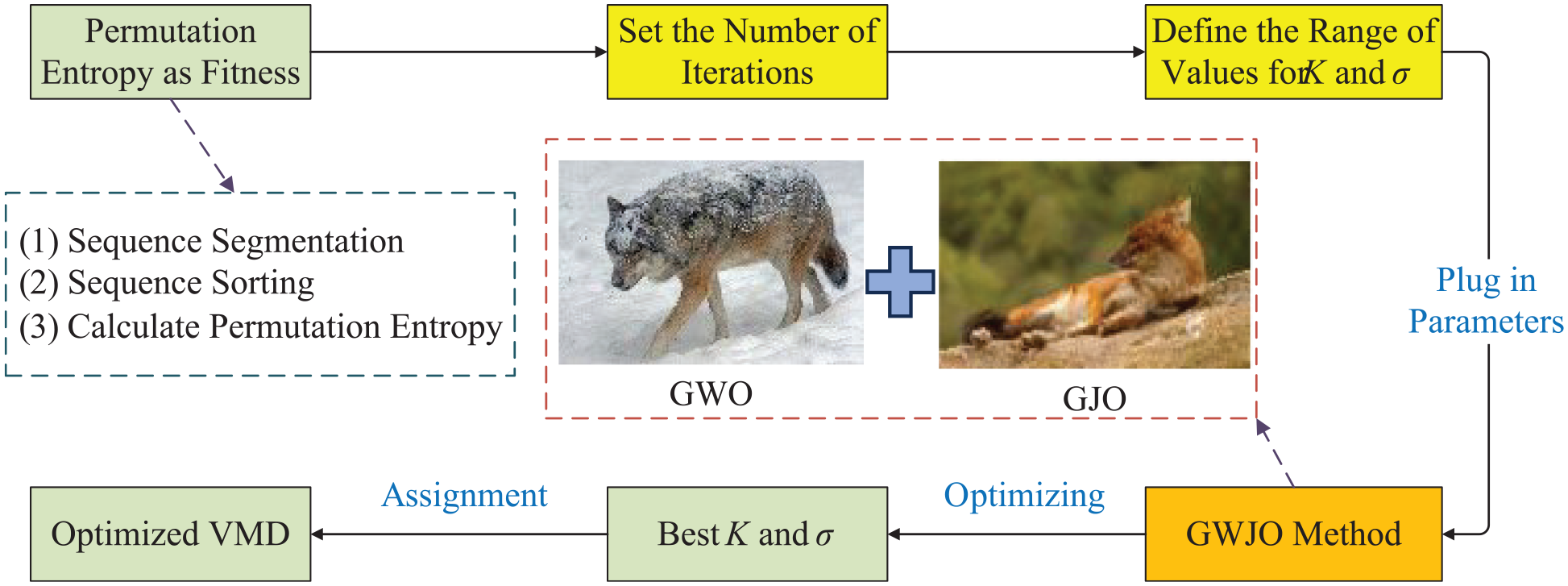
Flowchart of VMD optimization based on the GWJO algorithm.

As shown in Figure 4, to implement the GWJO algorithm, it is necessary to first set the key parameters, such as population size and maximum number of iterations, to ensure the effectiveness and convergence of the algorithm. After determining these parameters, specific iteration conditions are set and fitness values are calculated. In GWJO, permutation entropy is chosen as the fitness function, which directly affects the optimization effect. During the iteration process, the algorithm updates the positions and fitness values of individuals based on the population status, gradually approaching the optimal solution, and finally outputs the optimal position and its fitness value.

Figure 5 shows the process of using GWJO to optimize VMD. First, initial conditions such as sampling frequency, period, and number of points are set for VMD, for example, a sampling frequency of 12 kHz and 2048 sampling points. At the same time, the number of iterations for GWJO is set to fully explore the search space. GWJO adjusts the parameter combinations of VMD to find the optimal parameter configuration to maximize permutation entropy. Once found, the optimal parameters are fed back into the VMD algorithm for further data processing and analysis. This strategy improves the performance, robustness, and accuracy of the VMD algorithm, helps better identify and separate fault signals, and enhances the precision and reliability of bearing fault diagnosis. Regarding how VMD data is fed into MAFCNN, modifications have been described in section “Training sample.”

Traditional CNN model

CNN represent a specialized class of feedforward artificial neural networks that autonomously distill features from input signals for the purpose of classification through the application of convolutional operations. Conventional CNN architectures are predominantly structured around three types of layers: convolutional layers, pooling layers, and dense layers. The convolutional layer’s function is to identify and extract features from the input data through the use of filtering techniques. In this article, after optimizing the VMD parameters with the GWJO optimization algorithm, the permutation entropy calculated from the decomposed IMF is used. The permutation entropy of each IMF obtained from the decomposition is taken as a sample input, with each sample being one-dimensional data. Therefore, a one-dimensional CNN is utilized in this research. The convolution kernel operation formula is as follows:

y_{n}^{m + 1} (i) = K_{n}^{m} \times x^{m} (i) + b_{n}^{m}

(31)

where K and b represent the weights and biases of the n-th filter and the m-th layer, respectively, while x denotes the i-th local input of the m-th layer.

In this study, the computational burden is significantly alleviated and the data dimensionality is kept low due to the utilization of a limited dataset per sample. Consequently, the inclusion of a pooling layer subsequent to the convolutional layer is deemed unnecessary.

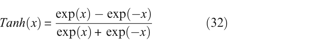
Activation functions can complicate the simple matrix multiplication in a linear manner, introducing nonlinearity into the neural networks to better handle nonlinear problems. The activation functions used in this paper are the Tanh function and the Softmax function. The graphs of the activation functions are shown in Figure 6, and their expressions are as follows:

(1) Tanh (Hyperbolic Tangent) function:

Tanh (x) = \frac{\exp (x) - \exp (- x)}{\exp (x) + \exp (- x)}

(32)

Figure 6.

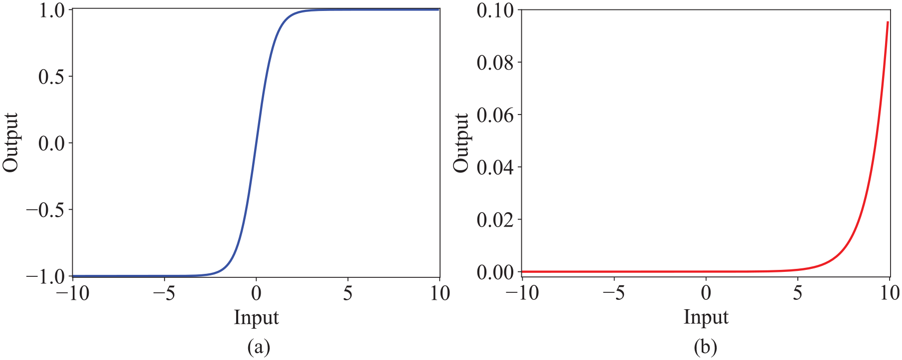
Activation function. (a) Tanh activation function graph and (b) Softmax activation function graph.

The Tanh function maps any real-valued number to a value between −1 and 1. It is often used in the hidden layers of neural networks because it provides a nonlinear transformation of the input and helps to ensure that the output is zero-centered, which can be beneficial for the training process.

(2) Softmax function:

Softmax (z_{i}) = \frac{\exp (z_{i})}{\sum_{j} \exp (z_{j})}

(33)

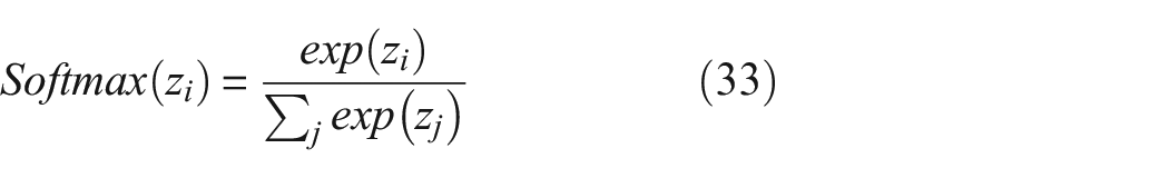
For a given vector of real numbers z=[z₁, z₂,…, z_K], the Softmax function returns a vector of values in the range [0, 1] that sum up to 1. It is commonly used in the output layer of classification problems to produce a probability distribution over different classes. The Softmax function turns output values into probabilities, summing to 1, ideal for multi-class classification where each neuron signifies a class score.

Proposed MAFCNN model

Deep learning methods have strong performance in the field of bearing fault detection, being able to automatically recognize and extract fault characteristics. Through the use of CNN within deep learning, various complex data can be effectively processed. The aim of this article is to combine GWJO-VMD with deep learning, allowing the neural networks to learn and automatically extract features from data obtained by the optimized algorithm, thereby displaying the health status of the bearing. Since the data obtained after GWJO-VMD decomposition is one-dimensional, one-dimensional convolution is used here.

Figure 7 presents the MAFCNN model, which incorporates convolutional kernels for the purpose of feature extraction and is equipped with a classifier module. This classifier is designed to sort the output into 10 distinct fault categories, labeled sequentially from 0 through 9. The MAFCNN model draws its inspiration from multi-scale convolutional neural networks (MCNNs) and marks a refinement over the traditional CNN model, thereby boosting the efficacy of feature extraction.³² While the MCNN relies on a variety of convolutional kernels to extract features, the MAFCNN opts for kernels with identical parameters but distinguishes itself by applying a diverse set of activation functions.

Figure 7.

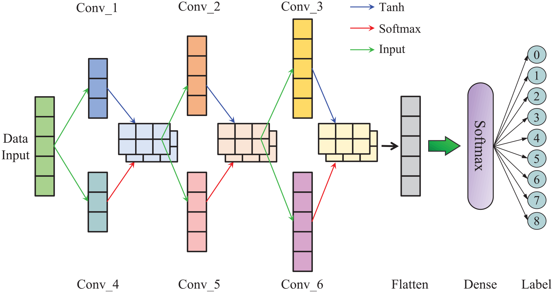
The network structure of MAFCNN.

We use the output results of the GWJO-VMD model as samples, with the size of each individual sample being (5 × 1), for automatic feature extraction and fault classification by inputting into this network. Conv_1, Conv_2, and Conv_3 serve as the main networks, employing the Tanh activation function. On this basis, Conv_4, Conv_5, and Conv_6 are added as auxiliary components, using the Softmax activation function. Since the data obtained through GWJO-VMD calculations is of similar size, the Softmax activation function can effectively differentiate between closely spaced data, highlighting the features. The corresponding convolutional kernels have completely identical parameters except for the activation functions, and they are integrated directly through tensor addition operations. This approach prevents the loss of features.

Finally, the Softmax function is used to convert the output of the neurons in the convolutional layers into the probability densities of 10 bearing fault categories. The description of the Softmax function is as follows:

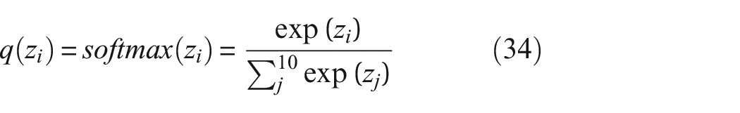
q (z_{i}) = softmax (z_{i}) = \frac{\exp (z_{i})}{\sum_{j}^{10} \exp (z_{j})}

(34)

where z represents the output of the i-th neuron.

The specific process of GWJO-VMD-MAFCNN

This section will demonstrate the processes of data preprocessing, feature extraction, and data training, as shown in Figure 8. During the optimization process of VMD using the GWJO algorithm, the GWJO combines the search parameter C of the GWO and the exploration system of the GJO, using permutation entropy as the fitness function.

Figure 8.

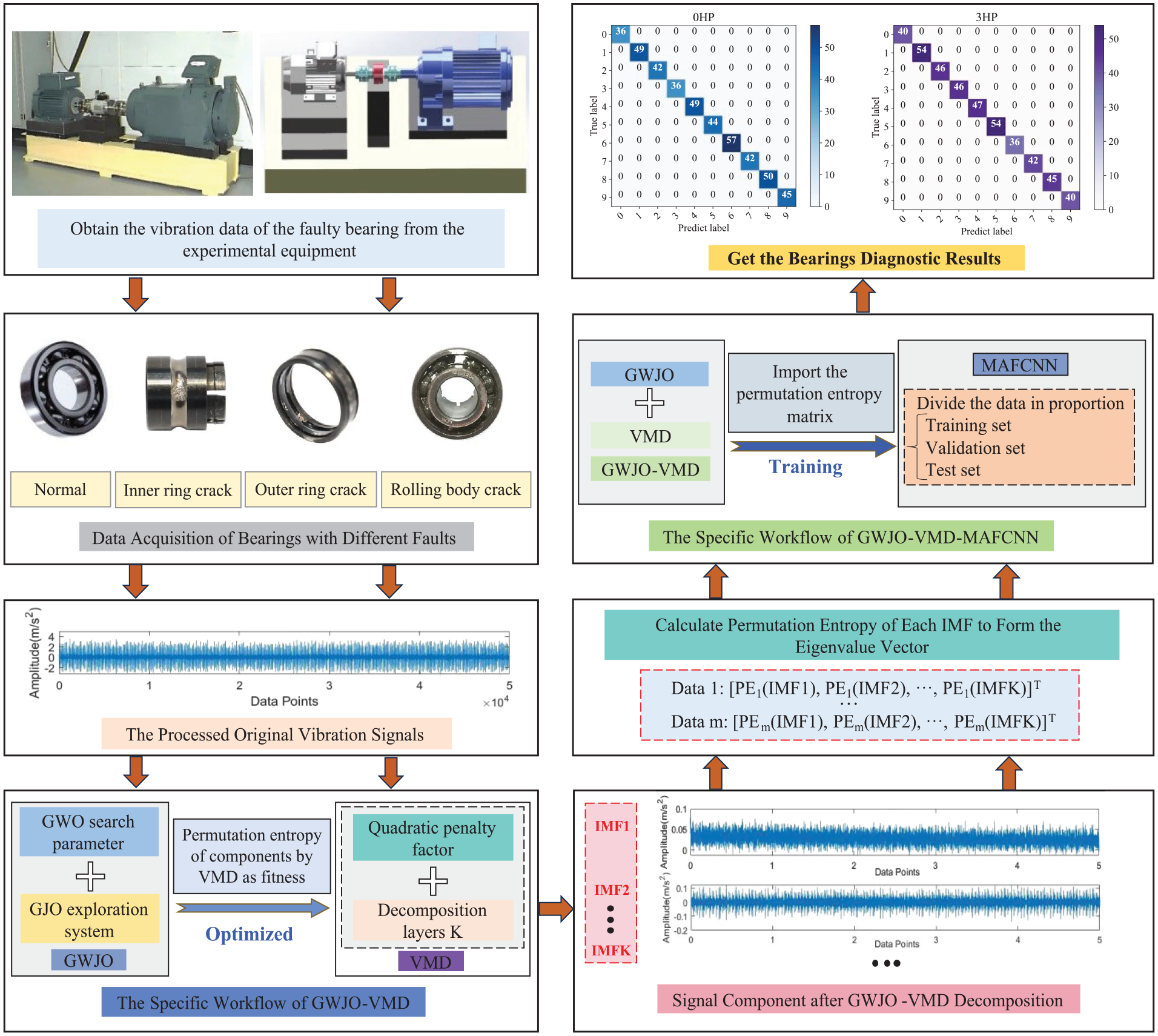
The specific process of GWJO-VMD-MAFCNN.

After the data-preprocessing phase, we proceed to the crucial phase of feature extraction. Here, key intrinsic traits of the data are pinpointed and distilled into a collection of features that encapsulate the core patterns and tendencies present within the dataset. It is worth highlighting that permutation entropy is utilized as the fitness function during this phase, enabling the conversion of the original signal into a one-dimensional matrix format, which is then leveraged for the extraction of meaningful features.

This method of processing fortifies the model’s reliability. Throughout the optimization phase, we have implemented the proposed GWJO algorithm to refine the parameters of the VMD. This optimization leads to an optimal representation of the data’s features, which in turn, significantly improves the model’s proficiency in diagnosing faults in bearings.

The exactly process of GWJO-VMD-MAFCNN as follows:

Step 1: Extract and convert sample points from fault datasets into a vibration signal.

Step 2: Import signals into the GWJO-VMD model and optimize σ and K using permutation entropy, and apply the optimized parameters to VMD for signal decomposition into IMF components.

Step 3: Calculate the permutation entropy for each IMF components to create a matrix.

Step 4: Use the one-dimensional permutation entropy vectors as samples, divide into training, validation, and test sets, and train MAFCNN for diagnostic outcomes.

Validate the feasibility of GWJO algorithm

Acquisition of test data

This test on bearing fault diagnosis utilized data from Case Western Reserve University under four load conditions. As shown in Figure 9, the testing procedure employs the electric discharge machining technique to induce single-point defects on the inner race, outer race, and roller of the test bearings, thereby mimicking three distinct fault conditions. The respective depths of these artificially induced faults are measured to be 0.1778, 0.3556, and 0.5334 mm. In this situation, the bearing generates a time-domain vibration signal with each rotation. To affirm the versatility of the GWJO in handling a broad spectrum of vibration signals, we have chosen to take 50,000 data points for the experimental validation. This large dataset allows us to thoroughly test the algorithm’s ability to accurately detect and analyze various fault conditions, ensuring its robustness and reliability in real-world applications.

Figure 9.

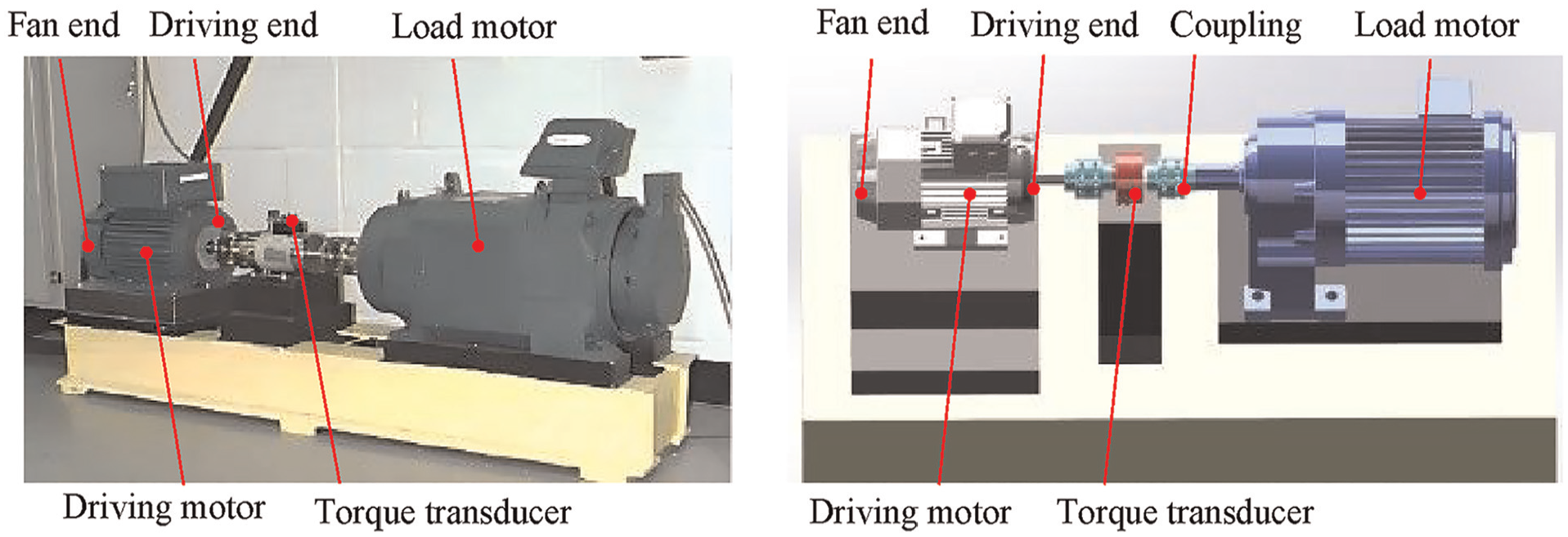
Bearing fault experiment device.

As shown in Figure 10, the test analyzed original vibration signals for four fault conditions (normal, outer ring fault, inner ring fault, and rolling body fault) and three fault diameters (0.1778, 0.3556, and 0.5334 mm) at a sampling frequency of 12 kHz under four load conditions (0, 1, 2, and 3 HP). This comprehensive setup allows us to thoroughly assess the algorithm’s ability to detect and differentiate between various fault types and severities under different operating conditions.

Figure 10.

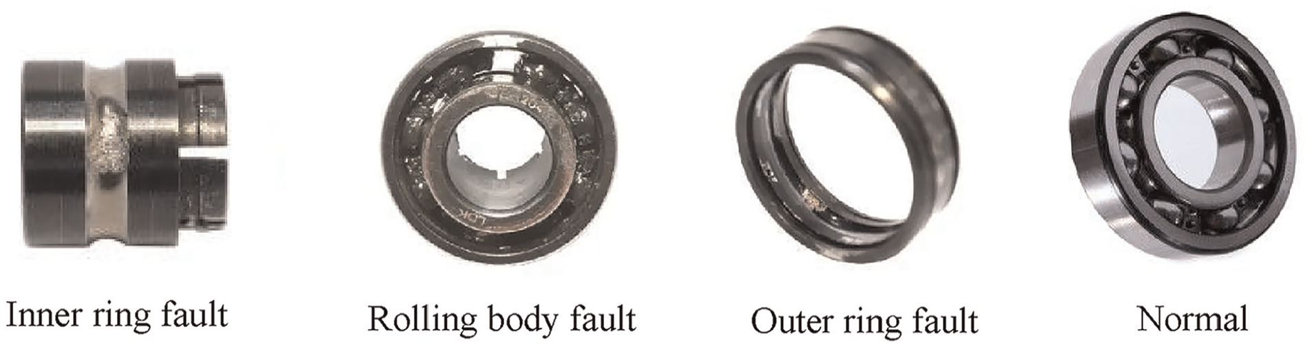
Four various types of bearing faults.

As shown in Figures 11 –13, the signal distinguishability of rolling bearings under various loads is relatively low for the same type of fault, as depicted in Figure 11(b)–(d). This similarity is further observed when comparing the spectrograms of the signals in Figure 11(b)–(d), where the four various loads yield nearly identical spectrograms. This lack of distinction is attributed to the experimental data showing minimal variation in rotational speeds across various loads, leading to a low frequency of characteristic pulse occurrences. Consequently, there is no significant variation in the spectral peak values of the fault characteristic frequencies within the spectrograms. However, when examining the time-domain waveforms of vibration signals from rolling bearings with different fault sizes, as shown in Figure 11 (b), (e), and (f), significant differences are noted. Faulty bearings exhibit more pronounced amplitude and distinct periodic vibration impacts compared to normal bearings, as illustrated in Figure 11 (a), (b), (g), and (h). In the spectrograms, specifically Figure 13(a), the spectrum of a normal bearing’s vibration signal is predominantly concentrated in the low-frequency range, with a relatively singular energy distribution. Figure 12(b) and (c) reveals that the energy from inner and outer race faults is primarily focused in the mid-frequency range, with low frequencies also being represented in the spectrogram. Figure 13(d) demonstrates that when a rolling element fails, there is a notable increase in energy across both low- and mid-frequency ranges, resulting in a more chaotic signal pattern.

Figure 11.

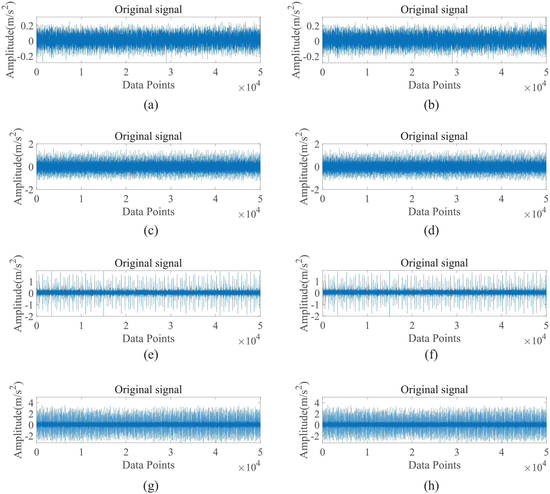
Time-domain diagrams of vibration signals for different types of rolling bearings under various fault conditions. (a) 0 HP, Normal, (b) 0 HP, Inner ring crack 0.1778 mm, (c) 1 HP, Inner ring crack 0.1778 mm, (d) 2 HP, Inner ring crack 0.1778 mm, (e) 0 HP, Inner ring crack 0.3556 mm, (f) 0 HP, Inner ring crack 0.5334 mm, (g) 0 HP, Outer ring crack 0.1778 mm, and (h) 0 HP, Rolling body crack 0.1778 mm.

Figure 12.

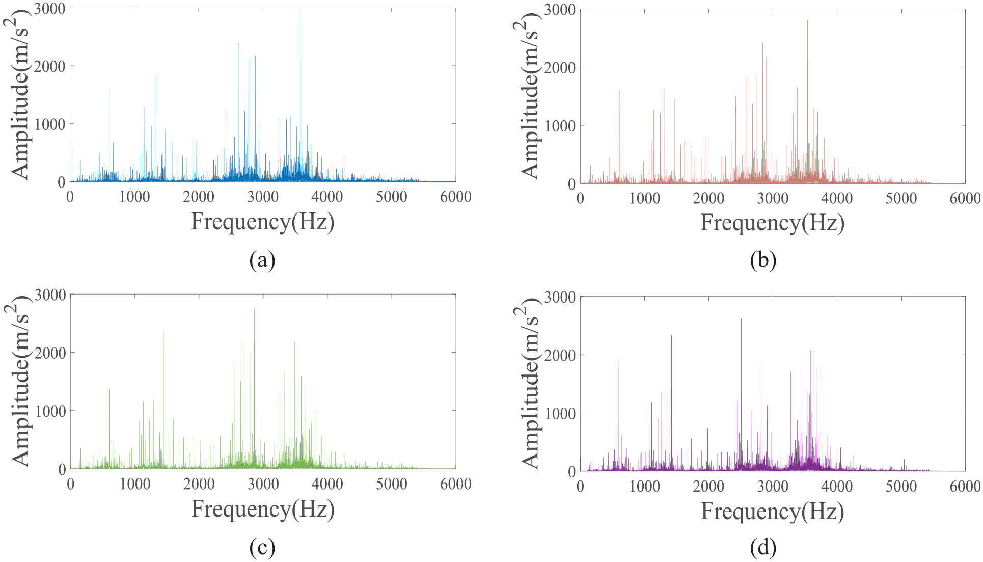
Vibration signal frequency-domain diagram of bearing inner race fault (with a fault diameter of 0.1778 mm) under various loads. (a) 0 HP, (b) 1 HP, (c) 3 HP, and (d) 4 HP.

Figure 13.

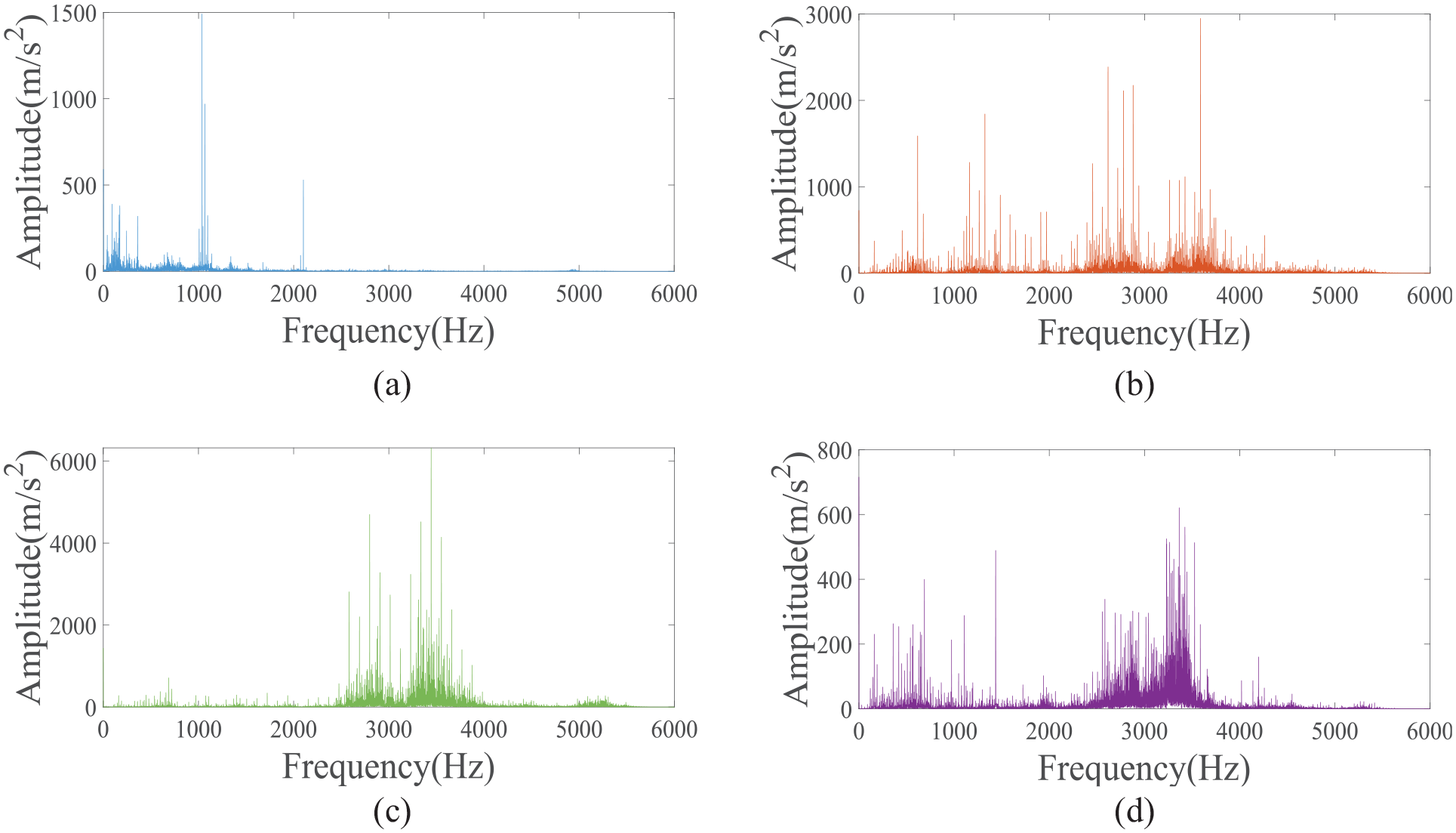
Frequency-domain diagrams of vibration signals for rolling bearings with different fault types (load at 0 HP and fault diameter of 0.1778 mm). (a) Normal bearings, (b) inner ring-cracked bearings, (c) outer ring-cracked bearings, and (d) rolling body-cracked bearings.

As depicted in Figure 13, while there exists some variation in the frequency-domain representations for various fault categories under identical load conditions and with the same fault diameter, it is important to note that these findings are predicated on ideal scenarios, and such distinctions might not hold true in practical applications. In the actual operating environment, the vibration signals may be affected by other factors, and these uncertainties may include environmental noise and the operating conditions of the equipment. It is therefore difficult to empirically differentiate directly between the frequency-domain plots of the raw data, and even if the technician is very experienced, artificial differentiation becomes unreliable in this case. Therefore, it becomes more important to adopt an optimization algorithm for feature extraction, which is an indispensable technique.

The process of verification

In the preceding part, we delved into the significance and essentiality of feature extraction, while the current segment concentrates on the validation of the suggested approach using spectrograms that encompass a dataset of 50,000 entries. We focus on the bearing faults under 0-HP load (with a fault depth of 0.1778 mm) as the subject of study, running 150 sets of data for each different fault type. We use the 2048 data collection points in the original signal for VMD decomposition. Afterwards, we use permutation entropy as the fitness function, which allows us to obtain the numerical matrix of permutation entropy derived from VMD decomposition. In the VMD approach, the critical parameters that dictate the decomposition of a set of intrinsic modal functions into the number of layers, K, and the penalty factor, σ, are pivotal. This article leverages the GWJO algorithm to ascertain these parameters. The values for σ and K have been derived from an average of 150 optimization runs on the initially gathered dataset. The optimal values for these parameters, as determined by the algorithm, are presented in Table 1.

Table 1.

The optimal parameters of GWJO-VMD.

Serial number	Fault types	Optimum solutions
		α	K
a	Normal	1747	6
b	Inner ring fault (fault diameter 0.1778 mm)	1567	6
c	Inner ring fault (fault diameter 0.3556 mm)	2287	6
d	Inner ring fault (fault diameter 0.5334 mm)	1901	6
e	Outer ring fault (fault diameter 0.1778 mm)	2246	6
f	Outer ring fault (fault diameter 0.3556 mm)	1667	6
g	Outer ring fault (fault diameter 0.5334 mm)	1702	5
h	Rolling body fault (fault diameter 0.1778 mm)	1901	6
i	Rolling body fault (fault diameter 0.3556 mm)	1796	6
j	Rolling body fault (fault diameter 0.5334 mm)	1748	6

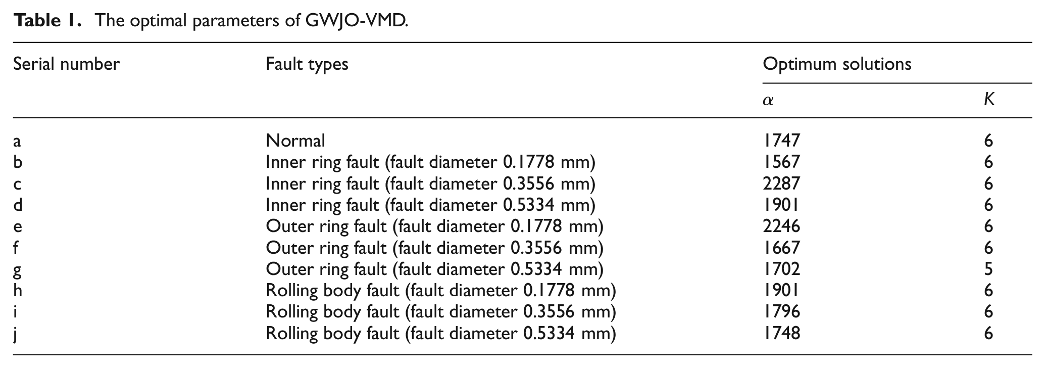
In order to substantiate the rationality of the two parameters we obtained (penalty factor σ and VMD decomposition level K), utilizing the optimal parameter set detailed in Table 1, we proceeded to generate the spectral representation of the original signal and each of its IMF components. In addition, for the purpose of convenient comparison, we also produced the vibration signal plots for both the original signal and its individual IMF components. Due to the large number of vibration signal collection points and their complexity, we conducted a study on the obtained spectrum to observe whether modal aliasing occurred. Figure 14 shows the spectrum of the rolling body and outer ring faults under the 0-HP load condition (fault diameter of 0.1778 mm).

Figure 14.

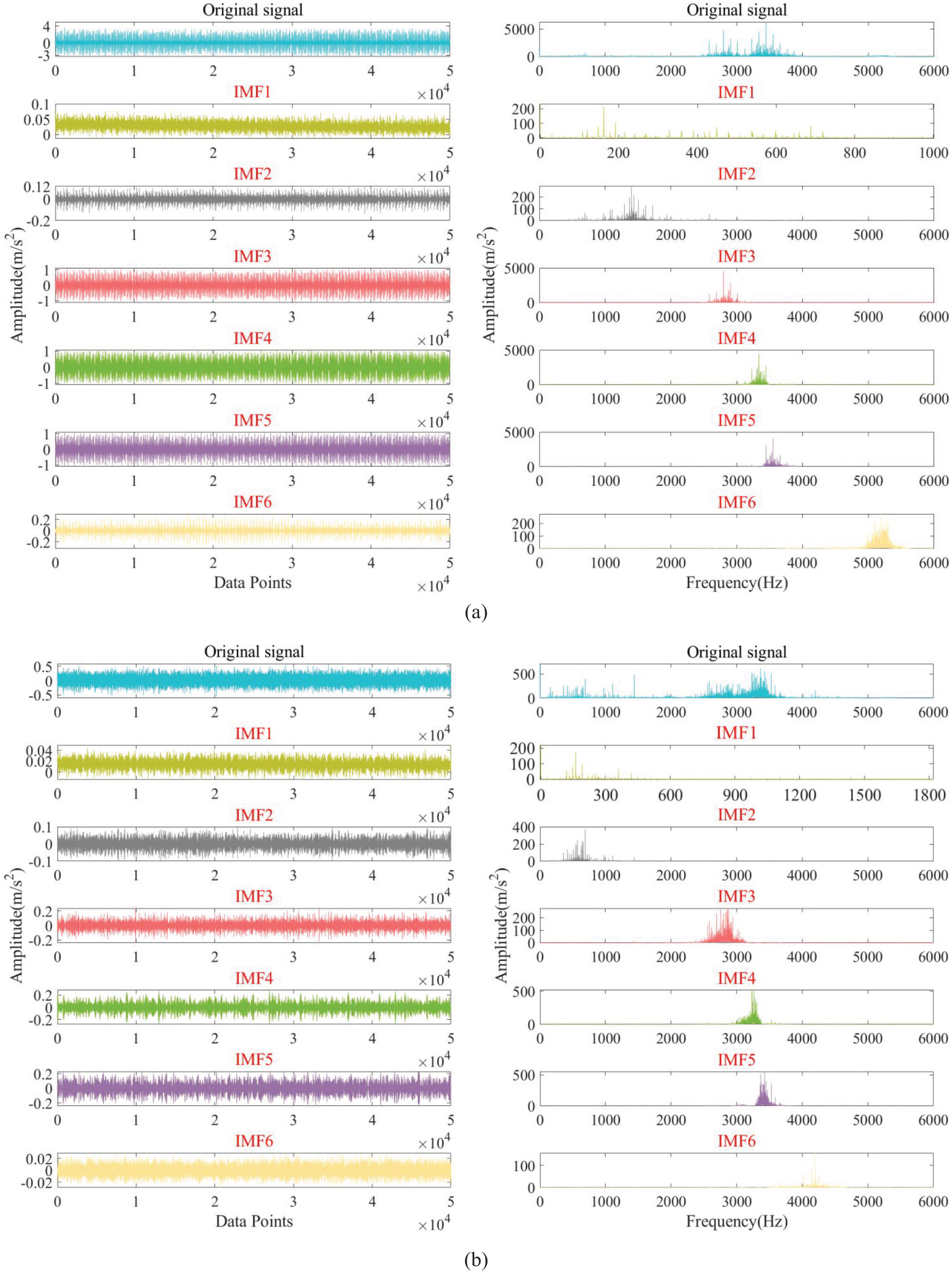
Time-domain waveform and spectrum diagram of vibration signal decomposed by GWJO-VMD. (a) Outer ring fault and (b) rolling body fault.

From Figure 14 (a) and (b), it can be observed that the frequency-domain diagrams of the multiple IMF components obtained from the decomposition of the original data do not exhibit modal aliasing. Therefore, this indicates that the optimization algorithm is feasible.

Experimental research

Data preprocessing and feature extraction

Data preprocessing

In this test, we employed a dataset from Case Western Reserve University, characterized by a sampling frequency of 12 kHz and comprising 2048 sampling points. Subsequently, VMD was applied to decompose these 2048 data points, yielding the permutation entropy of each resulting IMF component, which was then utilized as a feature vector. Specifically, we ran 150 sets for each condition combination under four fault conditions (normal, outer ring crack, inner ring crack, and rolling body crack), different degrees of damage (fault diameters of 0.1778, 0.3556, and 0.5334 mm), and various loads (0, 1, 2, and 3 HP). After that, the optimized penalty factor α and VMD decomposition level K are reintroduced into VMD, and the permutation entropy obtained from each set of IMF components is regarded as a sample. Each time, 50 samples are imported into the MAFCNN for training.

As illustrated in Figure 15, this test gathered vibration signals across 2048 data points. The normal bearing’s vibration signal (Figure 15(a)) is observed to be quite stable, with a minor amplitude and no significant fluctuations. In contrast, the signals from the faulty bearings (Figure 15(b)–(d)) present noticeable divergences from the normal ones. The time-domain waveforms of the faulty bearings’ vibrations exhibit higher amplitudes accompanied by clear periodic impacts. Despite the variance in the time-domain plots for the different faults, discerning specific fault characteristics is challenging. Consequently, a more refined approach to signal modal decomposition is required to further isolate and extract the distinctive features of each vibration signal.

Figure 15.

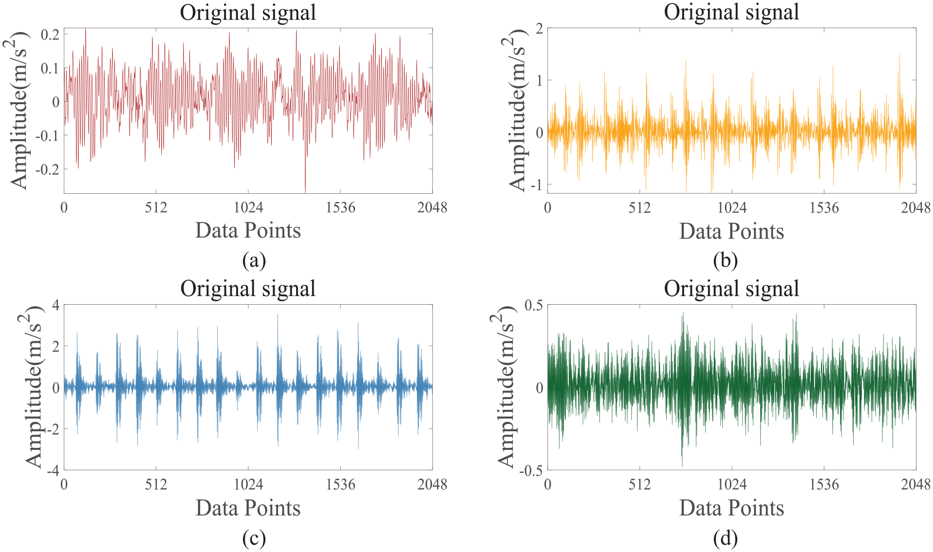
Under 0 HP, the time-domain waveforms of vibration signals from different faulty bearings. (a) Normal bearings, (b) inner ring-cracked bearings, (c) outer ring-cracked bearings, and (d) rolling body-cracked bearings.

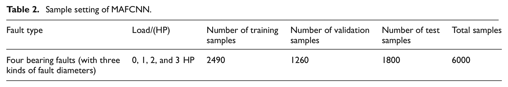
Before neural network training, setting the number of samples is an important matter. There are 150 sets of permutation entropy one-dimensional vectors for each fault state, including the following fault conditions: normal, inner ring fault (fault diameter 0.1778 mm), inner ring fault (fault diameter 0.3556 mm), inner ring fault (fault diameter 0.5334 mm), outer ring fault (fault diameter 0.1778 mm), outer ring fault (fault diameter 0.3556 mm), outer ring fault (fault diameter 0.5334 mm), rolling body fault (fault diameter 0.1778 mm), rolling body fault (fault diameter 0.3556 mm), and rolling body fault (fault diameter 0.5334 mm). Therefore, there are a total of 1500 sets of data under each load, and with four types of loads, there are a total of 6000 sets of data. In the first step, we initially divide the test set and its proportion into a 7:3 ratio, allocating 30% of the total as the test set. Subsequently, from the remaining 70% of the entire dataset, we proceed to split it into training and validation subsets in a 7:3 ratio. The precise allocation of this division is detailed in Table 2.

Table 2.

Sample setting of MAFCNN.

Fault type	Load/(HP)	Number of trainingsamples	Number of validationsamples	Number of testsamples	Total samples
Four bearing faults (with threekinds of fault diameters)	0, 1, 2, and 3 HP	2490	1260	1800	6000

Signal decomposition and feature extraction

After iterating 40 times on bearings in different fault states, the adaptability curves of the GWO (grey wolf optimization), GJO (golden jackal optimization), and GWJO algorithms in optimizing VMD parameters are analyzed and compared. This can verify the feasibility and adaptability of GWJO in optimizing VMD parameters.

As shown in Figure 16(a) and (b), it can be observed that GJO converges faster in some cases, yet it may fall into local optima. In contrast, GWO demonstrates good global search capabilities and relatively good convergence speed. However, as Figure 16(d) illustrates, GWO may also fall into local optima in certain situations. Therefore, to possess good global search capabilities without falling into local optima and to have faster convergence speed in more cases, GWJO was developed by combining the advantages of both GWO and GJO. Compared to GJO and GWO, GWJO not only has strong global search capabilities but also has better adaptability. As shown in Figure 16, under different fault conditions, GWJO can effectively find its VMD parameters without falling into local optima, which proves its good adaptability and practicality. Additionally, as depicted in Figure 16(c), GWJO maintains the fast convergence speed characteristic of GJO while ensuring global search capabilities. This demonstrates the strong adaptability and practicality of GWJO.

Figure 16.

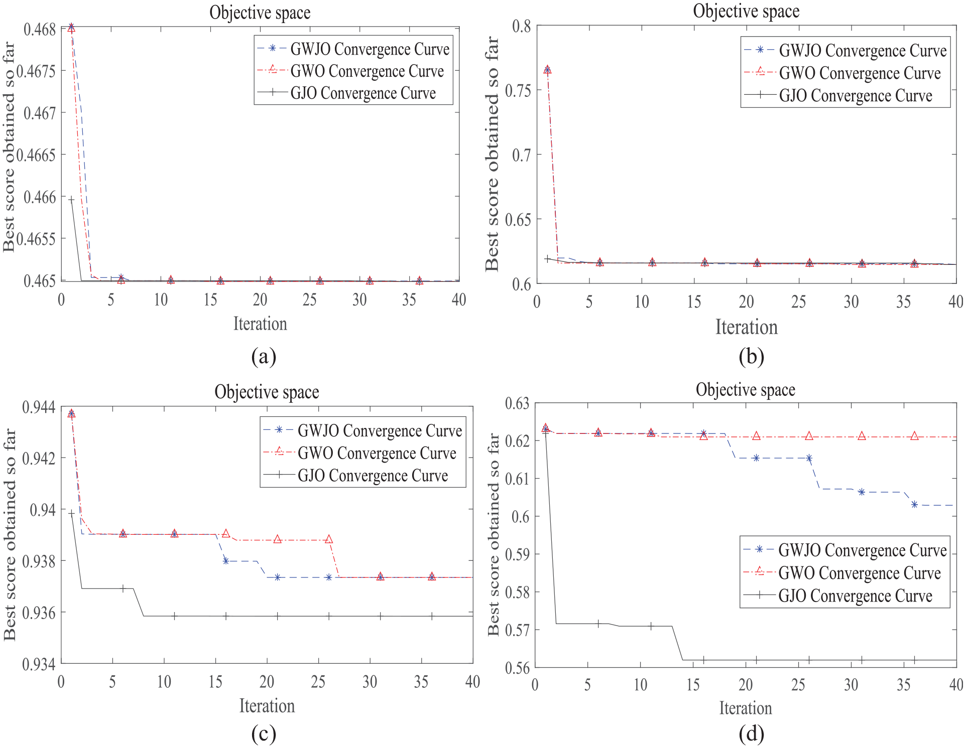
GWO, GJO, and GWJO respectively optimize the VMD fitness curves for different faults. (a) Normal bearings, (b) inner ring-cracked bearings, (c) outer ring-cracked bearings, and (d) rolling body-cracked bearings.

In the content of signal decomposition, we obtained the optimal σ and K values from Table 1, and at the same time collected 2048 data points. These two parameters were then brought back into the VMD, and six IMF components were obtained from the VMD decomposition. This also demonstrates the feasibility of GWJO, and we can observe whether there is any modal aliasing. The original data time-domain and frequency-domain graphs we obtained are shown in Figure 17.

Figure 17.

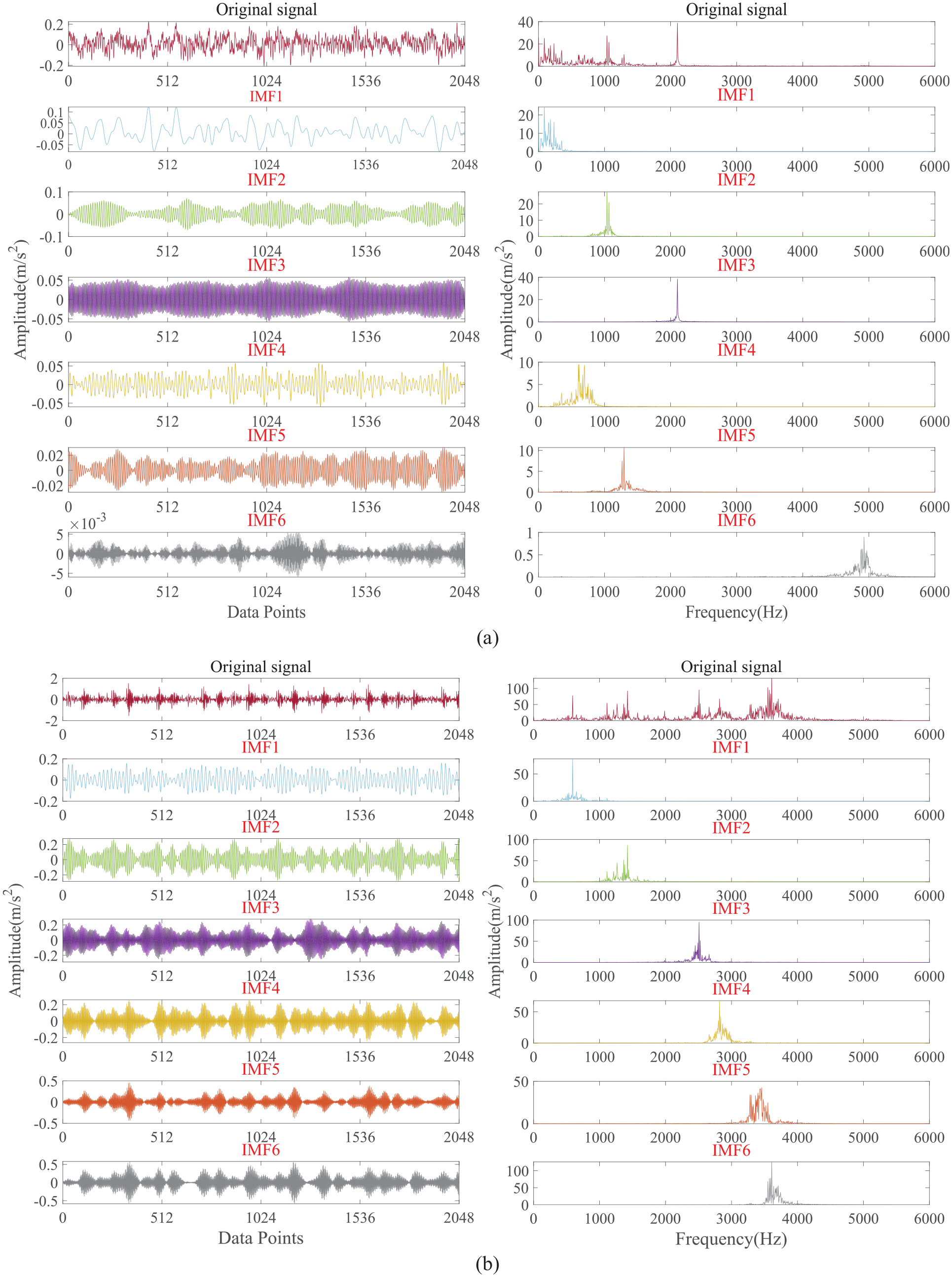
Optimize the VMD decomposition of vibration signals with different fault types under 3 HP in the time-domain waveform and spectrum. (a) Normal bearings and (b) inner ring-cracked bearings.

As shown in Figure 17, when we previously used GWJO-VMD to decompose the original data with 50,000 sampling points, there was no occurrence of modal aliasing; now, using the same method to decompose 2048 sampling points, modal aliasing will not occur either. This further verifies the feasibility of the GWJO algorithm.

In the content of feature extraction, we take each set of extracted permutation entropy as a feature vector D_v. The subsequent steps outline how to integrate it as a sample for training within the neural networks. The expression for D_v is as follows:

D_{v} = {[PE (IMF), PE (IMF), PE (IM F_{3}), \dots, PE (IM F_{n})]}^{T}

(35)

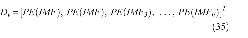
where n represents any positive integer.

Although permutation entropy values may have some distinguishability among different fault types, the actual situation is more complex. Therefore, it is unreasonable to rely solely on experience for judgment; we should employ more precise methods for classification.

Training based on MAFCNN

Training sample

According to the data-processing procedure in section “Data preprocessing,” we obtained the permutation entropy of 10 types of bearing faults under four different load conditions. In complex situations, it is challenging to directly identify the type of bearing fault through these permutation entropies. Therefore, we introduce a method based on deep learning neural networks that automatically extract features. Since after VMD decomposition, each group of samples contains 5–6 IMF components, to improve the model’s generalization ability, we uniformly take the first 5 IMF components as input data, with 150 sets for each type of fault, totaling 6000 sets for the 4 types of loads. Among them, 70% is designated for both training and validation, with the remaining 30% earmarked for testing. Within this training and validation subset, a 70–30 split is applied, with 70% constituting the training set and the remaining 30% serving as the validation set. Therefore, we provide 2490 sets for training samples, 1260 sets for validation samples, and 1800 sets for test samples. Notably, only the training and validation sets are used in model training; the test set does not participate in network training and is solely used to evaluate network performance. Thus, the test set represents unseen data for the network. We use the accuracy of the network on the test set to measure network performance, which effectively determines whether the network has merely memorized the training data or truly learned the underlying features. We use accuracy, precision, recall, and F1 score to evaluate the model:

Accuracy = \frac{TP + TN}{TP + FP + FN + TN}

(36)

Precision = \frac{TP}{TP + FP}

(37)

Recall = \frac{TP}{TP + FN}

(38)

F 1 = \frac{2 \times Precision \times Recall}{Precison + Recall}

(39)

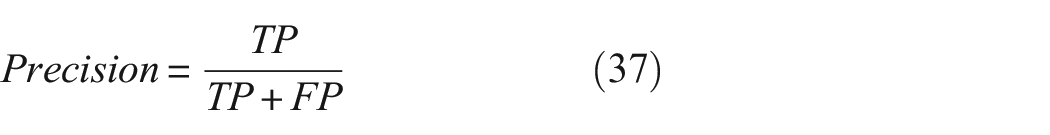
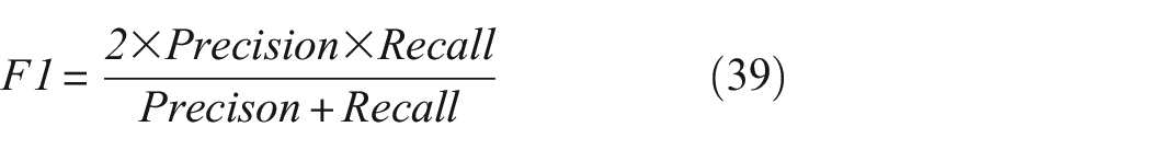
where TP stands for True Positive, FN for False Negative, TN for True Negative, and FP for False Positive.

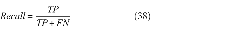
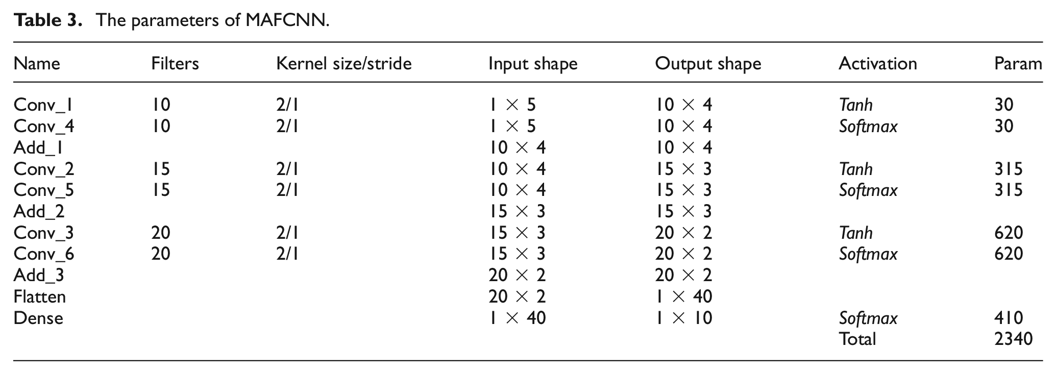
Parameter settings of the MAFCNN

The configuration of parameters for the proposed MAFCNN is detailed in Table 3. The Add_1, Add_2, and Add_3 layers are used to directly add the values at the corresponding positions of the feature maps obtained by convolution, instead of joining feature maps of the same shape as in Concat (Concat operation in the U-net network). This does not change the shape of the feature maps. The “Flatten” layer reduces the size of the feature map, allowing it to be fed directly into dense for classification. After the Flatten layer, a dropout layer is set to prevent overfitting and update the weights using a backpropagation mechanism. the parameter of the dropout layer is set to 0.2, which should not be too high to reduce the likelihood of underfitting during the training process. The mean square error is used as a loss function during training. We use the TensorFlow library in Python, and both Keras and TensorFlow versions are 2.15.0. The Adam optimizer built into Keras is used, with the learning rate which is set to 0.006 and the training period which is set to 600. The training process was conducted on a high-performance laptop equipped with an Intel i7-12700H CPU and a GeForce RTX 3060 GPU. It is important to highlight that, despite the presence of a powerful GPU, the training was specifically executed on the CPU. This decision was made to optimize the training process for certain computational tasks that are more efficiently handled by the CPU’s architecture. The efficacy of training might be influenced by the stochastic assignment of training and test datasets, as well as by the random initialization of weights and biases. To bolster the reliability of the test outcomes and to assess the consistency of the model’s accuracy, five distinct test runs were conducted with identical parameter settings. This approach lets us gauge model consistency by verifying accuracy variance across five trials.

Table 3.

The parameters of MAFCNN.

Name	Filters	Kernel size/stride	Input shape	Output shape	Activation	Param
Conv_1	10	2/1	1 × 5	10 × 4	Tanh	30
Conv_4	10	2/1	1 × 5	10 × 4	Softmax	30
Add_1			10 × 4	10 × 4
Conv_2	15	2/1	10 × 4	15 × 3	Tanh	315
Conv_5	15	2/1	10 × 4	15 × 3	Softmax	315
Add_2			15 × 3	15 × 3
Conv_3	20	2/1	15 × 3	20 × 2	Tanh	620
Conv_6	20	2/1	15 × 3	20 × 2	Softmax	620
Add_3			20 × 2	20 × 2
Flatten			20 × 2	1 × 40
Dense			1 × 40	1 × 10	Softmax	410
					Total	2340

Training results

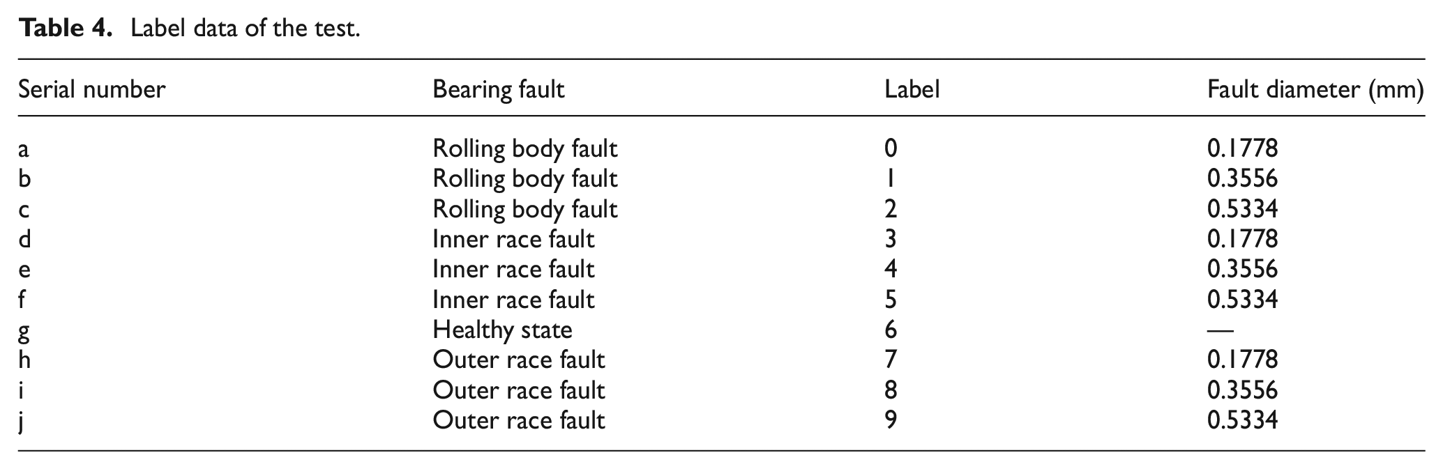
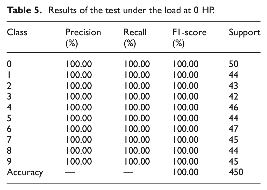
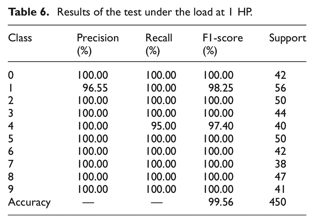
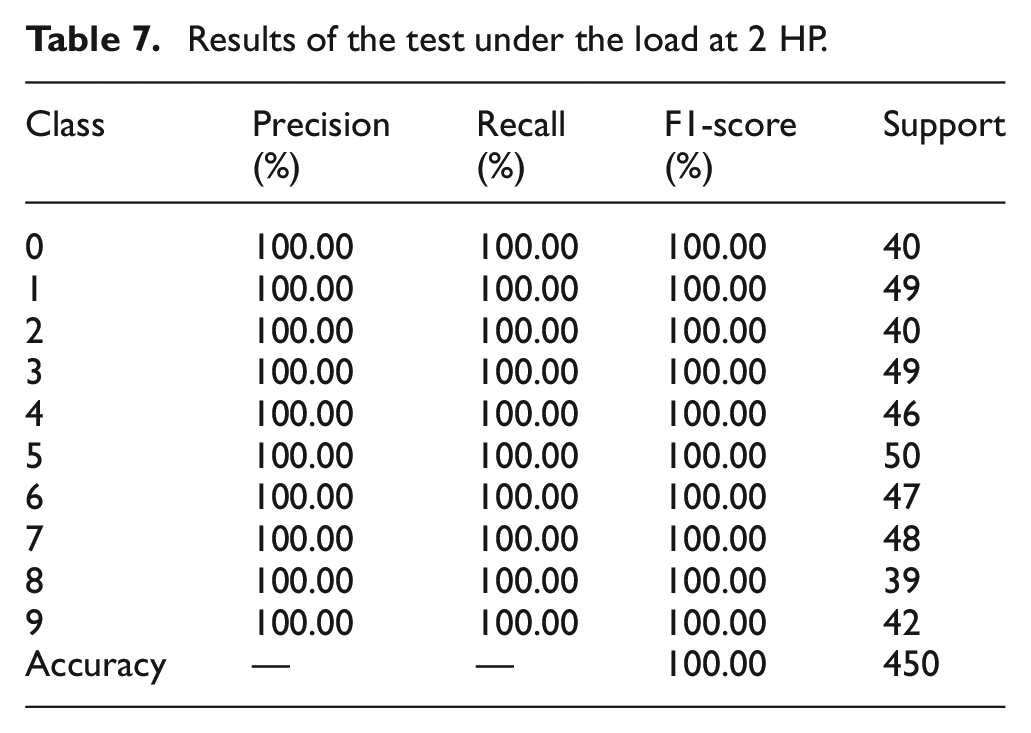
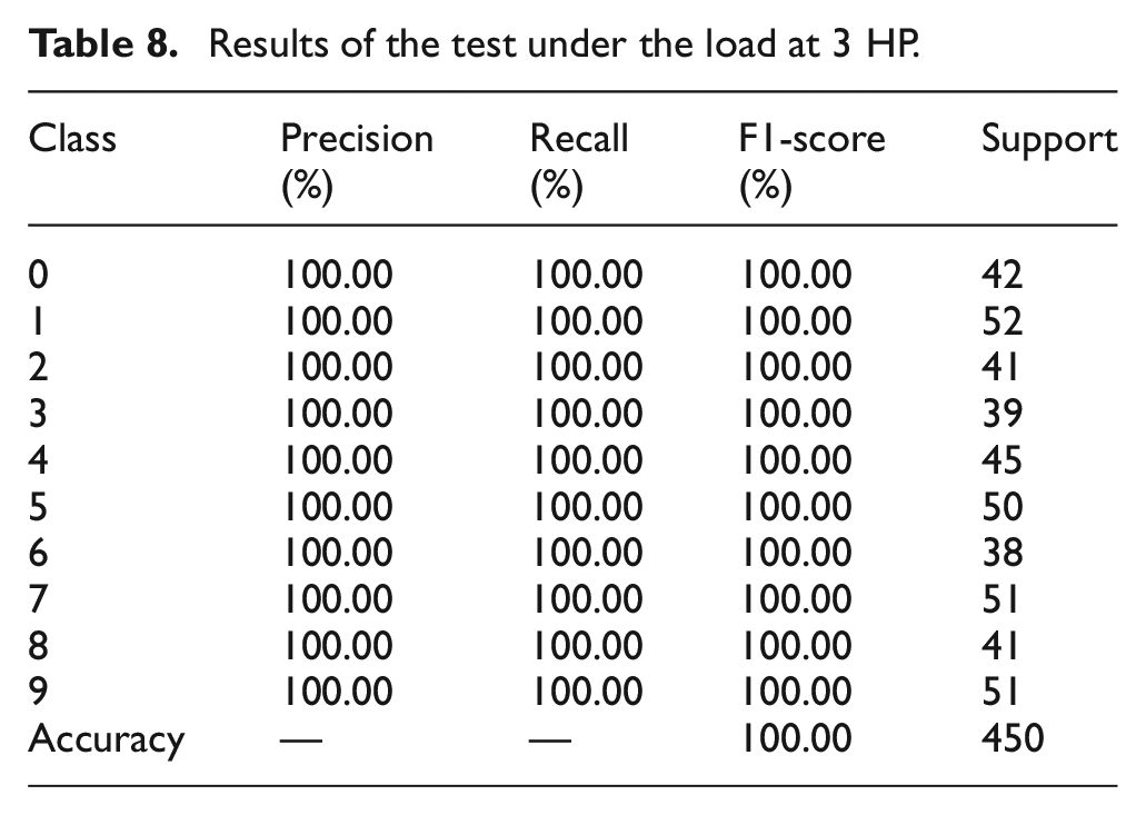
Table 4 presents the fault labels for various types of rolling bearings and the respective dimensions of each fault category throughout the training phase of the MAFCNN. Figure 18 shows the test accuracy in five trials under four different load conditions. The test accuracy for loads of 0 and 3 HP both reached 100%; for the 1-HP load, the test accuracy was no less than 98.44%, with a maximum of 100%; under the 2-HP load, there was only one trial with an accuracy of 99.56%, while all other trials achieved an accuracy of 100%. Overall, the five trials indicate that the MAFCNN can train to produce good results under the four various loads. Tables 5 –8 shows the classification of each fault type by the MAFCNN, represented by Precision, Recall, F1-Score, and Accuracy. The MAFCNN has a very strong recognition ability for the IMF components obtained from the GWJO-VMD operation on the bearing data under various loads of 0, 2, and 3 HP, with a test accuracy that can reach 100%. However, when identifying under the 1-HP load, for labels 1 and 4 (label 1 is ball crack with fault diameter 0.3556 mm, label 4 is inner race crack with fault diameter 0.3556 mm), the F1-Scores were 98.25% and 97.40%, respectively. In summary, the training results validate that the proposed MAFCNN framework can effectively classify data after GWJO-VMD decomposition. The GWJO-VMD-MAFCNN framework presented in this article can effectively detect various bearing faults.

Table 4.

Label data of the test.

Serial number	Bearing fault	Label	Fault diameter (mm)
a	Rolling body fault	0	0.1778
b	Rolling body fault	1	0.3556
c	Rolling body fault	2	0.5334
d	Inner race fault	3	0.1778
e	Inner race fault	4	0.3556
f	Inner race fault	5	0.5334
g	Healthy state	6	—
h	Outer race fault	7	0.1778
i	Outer race fault	8	0.3556
j	Outer race fault	9	0.5334

Figure 18.

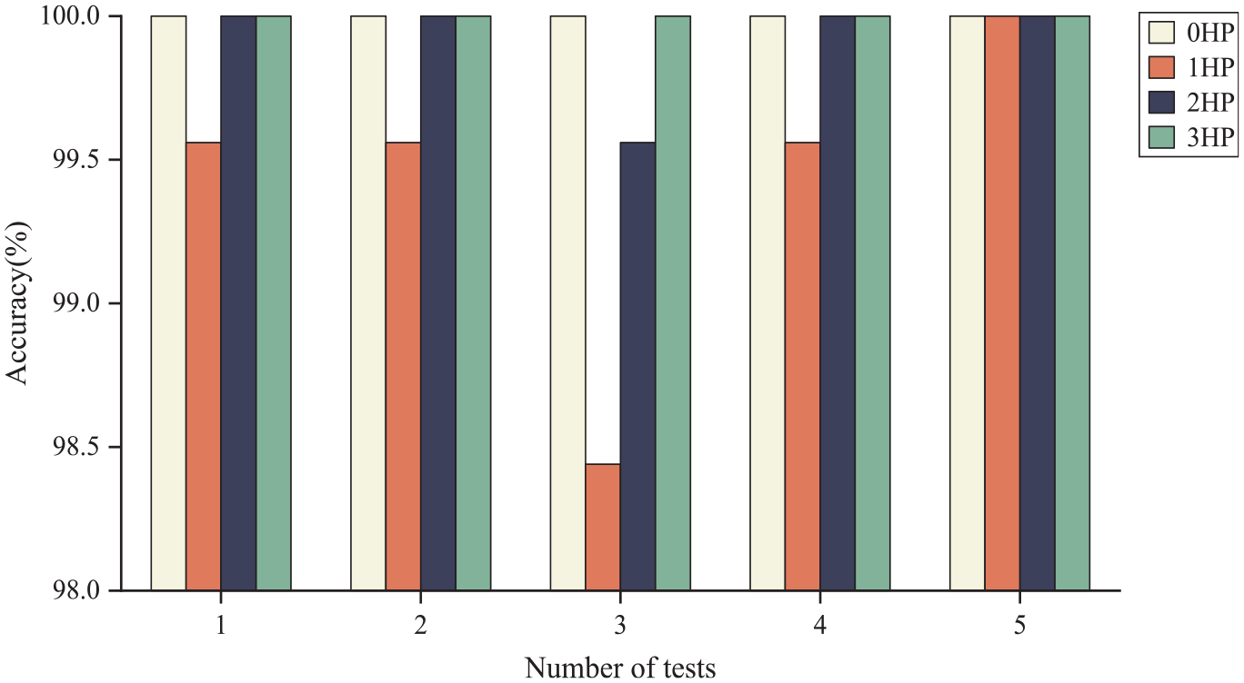
The diagnosis accuracy of five trials which under four various loads (0, 1, 2, and 3 HP).

Table 5.

Results of the test under the load at 0 HP.

Class	Precision(%)	Recall(%)	F1-score(%)	Support
0	100.00	100.00	100.00	50
1	100.00	100.00	100.00	44
2	100.00	100.00	100.00	43
3	100.00	100.00	100.00	42
4	100.00	100.00	100.00	46
5	100.00	100.00	100.00	44
6	100.00	100.00	100.00	47
7	100.00	100.00	100.00	45
8	100.00	100.00	100.00	44
9	100.00	100.00	100.00	45
Accuracy	—	—	100.00	450

Table 6.

Results of the test under the load at 1 HP.

Class	Precision(%)	Recall(%)	F1-score(%)	Support
0	100.00	100.00	100.00	42
1	96.55	100.00	98.25	56
2	100.00	100.00	100.00	50
3	100.00	100.00	100.00	44
4	100.00	95.00	97.40	40
5	100.00	100.00	100.00	50
6	100.00	100.00	100.00	42
7	100.00	100.00	100.00	38
8	100.00	100.00	100.00	47
9	100.00	100.00	100.00	41
Accuracy	—	—	99.56	450

Table 7.

Results of the test under the load at 2 HP.

Class	Precision(%)	Recall(%)	F1-score(%)	Support
0	100.00	100.00	100.00	40
1	100.00	100.00	100.00	49
2	100.00	100.00	100.00	40
3	100.00	100.00	100.00	49
4	100.00	100.00	100.00	46
5	100.00	100.00	100.00	50
6	100.00	100.00	100.00	47
7	100.00	100.00	100.00	48
8	100.00	100.00	100.00	39
9	100.00	100.00	100.00	42
Accuracy	—	—	100.00	450

Table 8.

Results of the test under the load at 3 HP.

Class	Precision(%)	Recall(%)	F1-score(%)	Support
0	100.00	100.00	100.00	42
1	100.00	100.00	100.00	52
2	100.00	100.00	100.00	41
3	100.00	100.00	100.00	39
4	100.00	100.00	100.00	45
5	100.00	100.00	100.00	50
6	100.00	100.00	100.00	38
7	100.00	100.00	100.00	51
8	100.00	100.00	100.00	41
9	100.00	100.00	100.00	51
Accuracy	—	—	100.00	450

As shown in Figure 19, the horizontal axis of the confusion matrix represents the fault types predicted by the model, while the vertical axis represents the actual fault types. The confusion matrices for the four load conditions show that almost all samples are located along the diagonal of the matrix, indicating a one-to-one correspondence between the predicted fault types and the actual fault types.

Figure 19.

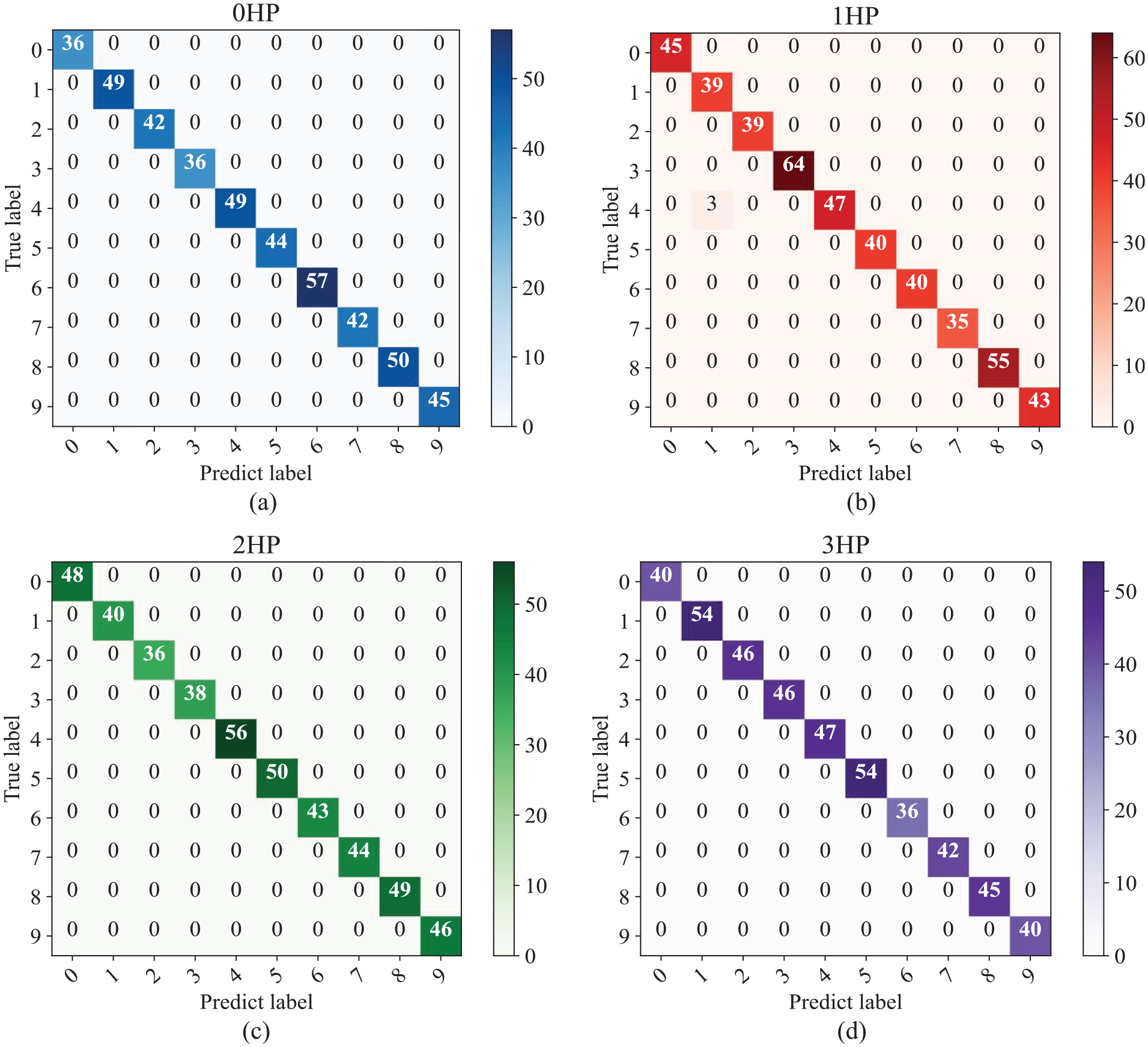
Results of confusion matrix under four various loads. (a) 0 HP, (b) 1 HP, (c) 2 HP, and (d) 3 HP.

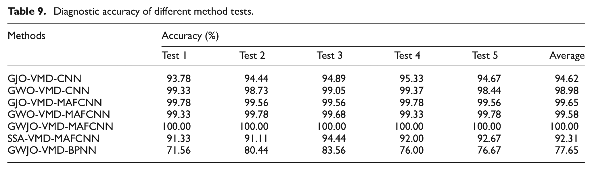
In this segment, we conducted a comparative analysis of seven different methods to elucidate the advantages of the proposed GWJO algorithm and MAFCNN. The methods compared include GWJO-VMD-BPNN, SSA-VMD-MAFCNN, GJO-VMD-CNN, GWO-VMD-CNN, GJO-VMD-MAFCNN, GWO-VMD-MAFCNN, and GWJO-VMD-MAFCNN. The results are shown in Table 9 and Figure 20. From the figures and tables, it can be observed that GWJO-VMD-MAFCNN achieved a 100% accuracy rate in all five tests. In contrast, the lowest accuracy among the seven methods was GWJO-VMD-BPNN, which is attributed to the stronger learning and classification capabilities of MAFCNN compared to other networks. The GWO algorithm has better global optimization capabilities, which results in higher accuracy compared to the GJO algorithm. It can be noted that the methods using CNN have a slightly lower final average accuracy rate than those using MAFCNN, indicating the superiority of the proposed MAFCNN. MAFCNN can increase the accuracy rate from 94.62% and 98.98% to above 99%. The reason why GWJO-VMD-MAFCNN can achieve a 100% accuracy rate is that the GWJO algorithm has stronger global optimization capabilities in certain situations. Comparing GWJO with GJO, GWO, and SSA, it can be seen that GWJO has a stronger global search ability than some similar algorithms. Other methods may fall into local optima in some cases, leading to a decrease in the final fault diagnosis accuracy rate. By combining GWJO with MAFCNN, the accuracy rate of the proposed model in this paper can always be maintained at 100%, demonstrating its strong stability and global optimization capabilities.

Table 9.

Diagnostic accuracy of different method tests.

Methods	Accuracy (%)
	Test 1	Test 2	Test 3	Test 4	Test 5	Average
GJO-VMD-CNN	93.78	94.44	94.89	95.33	94.67	94.62
GWO-VMD-CNN	99.33	98.73	99.05	99.37	98.44	98.98
GJO-VMD-MAFCNN	99.78	99.56	99.56	99.78	99.56	99.65
GWO-VMD-MAFCNN	99.33	99.78	99.68	99.33	99.78	99.58
GWJO-VMD-MAFCNN	100.00	100.00	100.00	100.00	100.00	100.00
SSA-VMD-MAFCNN	91.33	91.11	94.44	92.00	92.67	92.31
GWJO-VMD-BPNN	71.56	80.44	83.56	76.00	76.67	77.65

Figure 20.

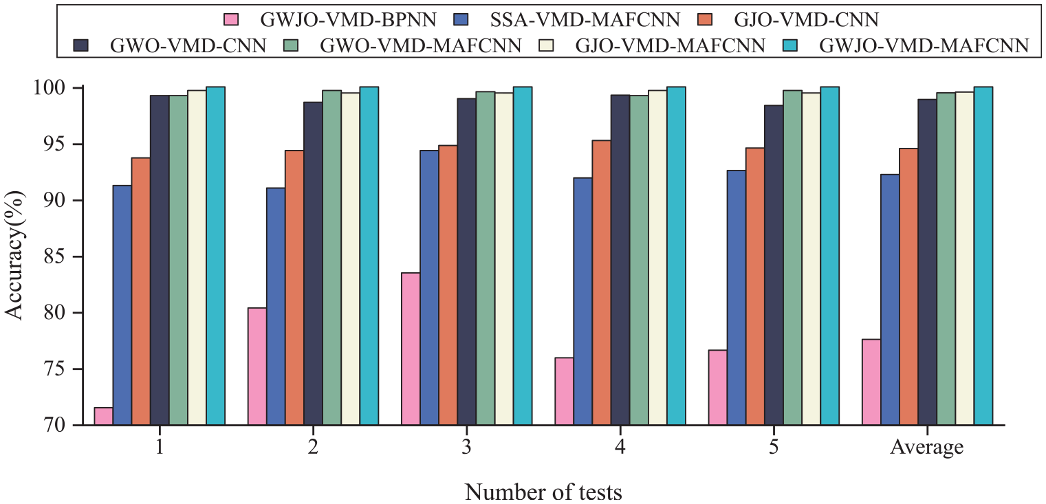
Test diagnostic accuracy.

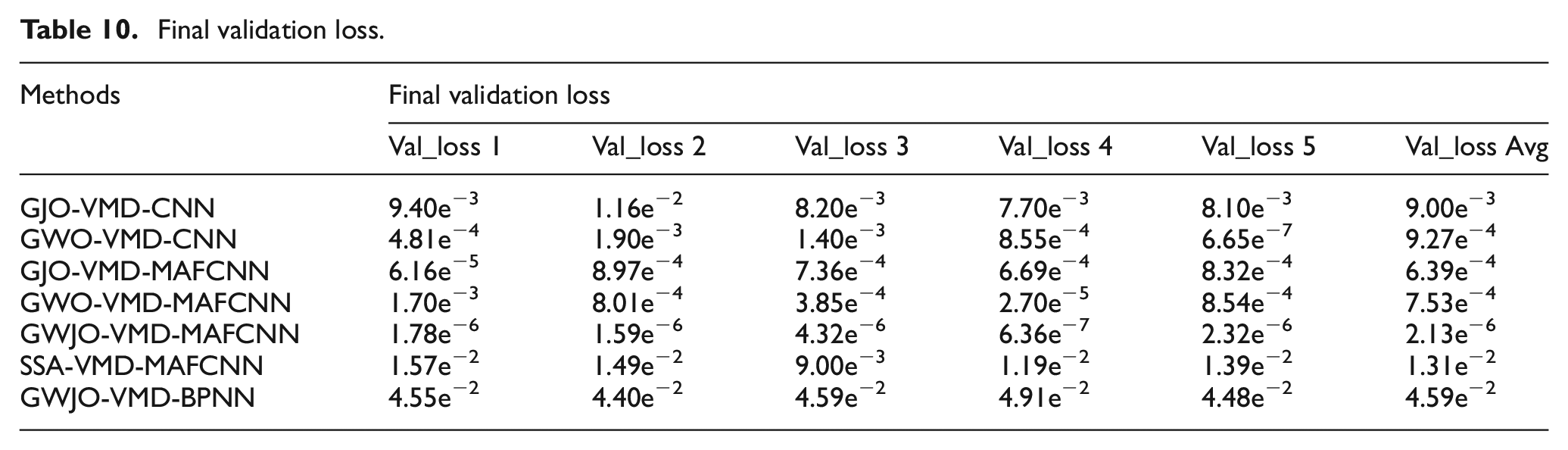
At the same time, we also obtained the validation loss after the completion of each test training, with the specific data shown in Table 10. This data represents the validation loss at the time when the model parameters were saved upon completion of training. The validation loss is the error of the model on the validation set. The lower the validation loss, the better the model performs on the validation set, indicating that the model can more accurately predict unseen data and possesses better generalization ability. By examining the validation loss, we can better understand why the MAFCNN exhibits superior fault recognition capabilities compared to other models. From Table 10, the average validation loss of GWJO-VMD-MAFCNN is the smallest, which means that the accuracy of our proposed method is the highest among the seven methods. Furthermore, the mean validation loss for the GJO-optimized CNN model stands at 9.00e⁻³, whereas for the MAFCNN model, it is 6.39e⁻⁴; for the GWO-optimized CNN model, the average validation loss is 9.27e⁻⁴, and for the GWO-optimized MAFCNN model, it is 7.53e⁻⁴. Additionally, SSA-VMD-MAFCNN and GWJO-VMD-BPNN showed poor validation loss performance. Overall, the proposed GWJO-VMD-MAFCNN model achieves high accuracy and outperforms other models.

Table 10.

Final validation loss.

Methods	Final validation loss
	Val_loss 1	Val_loss 2	Val_loss 3	Val_loss 4	Val_loss 5	Val_loss Avg
GJO-VMD-CNN	9.40e⁻³	1.16e⁻²	8.20e⁻³	7.70e⁻³	8.10e⁻³	9.00e⁻³
GWO-VMD-CNN	4.81e⁻⁴	1.90e⁻³	1.40e⁻³	8.55e⁻⁴	6.65e⁻⁷	9.27e⁻⁴
GJO-VMD-MAFCNN	6.16e⁻⁵	8.97e⁻⁴	7.36e⁻⁴	6.69e⁻⁴	8.32e⁻⁴	6.39e⁻⁴
GWO-VMD-MAFCNN	1.70e⁻³	8.01e⁻⁴	3.85e⁻⁴	2.70e⁻⁵	8.54e⁻⁴	7.53e⁻⁴
GWJO-VMD-MAFCNN	1.78e⁻⁶	1.59e⁻⁶	4.32e⁻⁶	6.36e⁻⁷	2.32e⁻⁶	2.13e⁻⁶
SSA-VMD-MAFCNN	1.57e⁻²	1.49e⁻²	9.00e⁻³	1.19e⁻²	1.39e⁻²	1.31e⁻²
GWJO-VMD-BPNN	4.55e⁻²	4.40e⁻²	4.59e⁻²	4.91e⁻²	4.48e⁻²	4.59e⁻²

Evaluate the generalization ability of GWJO

To demonstrate the robustness and generalization ability of the GWJO-VMD-MAFCNN model in fault diagnosis, we selected the bearing dataset from Southeast University for verification and training. This dataset includes five fault conditions: Ball fault, Inner ring fault, Outer ring fault, Combination fault on both inner ring and outer ring, and Health working state, under operating conditions of 1200-rpm speed and 0-Nm load. For each fault condition, 200 sets of permutation entropy data were obtained, resulting in a total of 1000 datasets. The data was divided according to the method described in section “Data preprocessing.” Furthermore, we obtained the training results and confusion matrix as shown in the following figure:

As shown in Figure 21(a), the confusion matrix represents the model’s classification results on the training set, with all data points lying on the diagonal of the matrix. This indicates that the model’s predictions are consistent with the true fault conditions, demonstrating that the model has a strong discriminative ability on the Southeast University bearing dataset. Figure 21(b) illustrates the training process of the model on the Southeast University bearing dataset, where the training accuracy reached a high level after 200 iterations.

Figure 21.

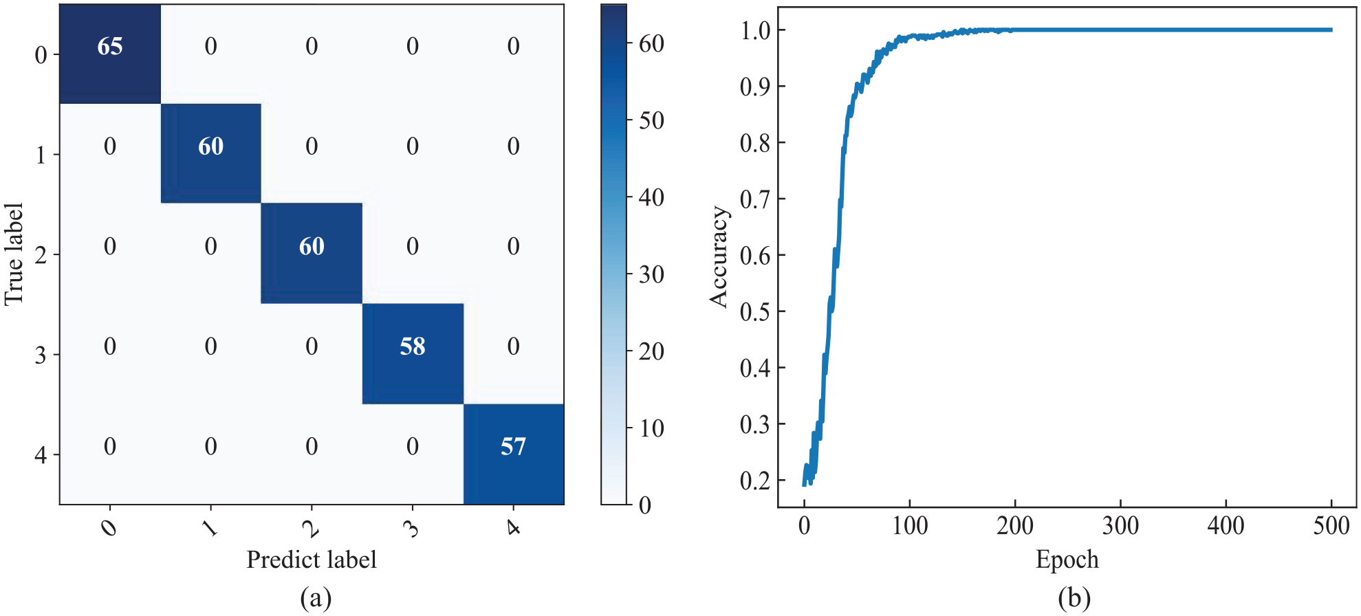
Testing results on the new dataset. (a) Confusion matrix and (b) iterative curve.

The GWJO-VMD-MAFCNN fault diagnosis model exhibits strong diagnostic capabilities both on the Case Western Reserve University bearing dataset and the Southeast University bearing dataset. This demonstrates that the model possesses significant robusts, capable of identifying various types, operating conditions, and fault scenarios of bearing vibration data.

Conclusions

In this article, GWJO-VMD-MAFCNN is used for bearing fault diagnosis analysis, where GWJO is employed to optimize the regularization parameter K and the penalty factor σ of VMD. The permutation entropy is used as the fitness function, and based on this, the permutation entropy matrix of the IMF obtained from VMD decomposition can be obtained. This matrix is then input into MAFCNN for training. Additionally, comparative tests are conducted to demonstrate the feasibility of the proposed method. The conclusions drawn are as follows:

During the verification tests, the GWJO-VMD method did not experience modal aliasing when using 50,000 data collection points from the original data; and in the subsequent experimental process, we used 2048 data collection points from the original data, which also did not experience modal aliasing. This indicates that the proposed GWJO algorithm performs well under both the extensive and local data collection points of the original data, demonstrating good feasibility.

The results of the training indicate that GWJO can effectively optimize the two parameters of VMD. The outcomes of the five training tests with GWJO-VMD-MAFCNN have all achieved a 100% accuracy rate, which is higher compared to other methods. This further proves the feasibility of GWJO and shows that the GWJO algorithm is more capable of global optimization than GJO, GWO, SSA, or other similar algorithms.

The training results and the final validation loss demonstrate that the proposed MAFCNN has stronger classification capabilities compared to the traditional CNN, and its final average validation loss is below the order of magnitude of 10e⁻⁴, reflecting its higher accuracy. Moreover, the results are even better when this method is applied to GWJO. The average validation loss for GWJO-VMD-MAFCNN has reached 2.13e⁻⁶. In addition, we use the bearing dataset from Southeast University to evaluate the generalization ability of the proposed method, and the final result shows that the proposed method in this paper has strong stability and generalization ability.

Footnotes

Appendix

CRediT authorship contribution statement

All authors contributed to the study conception and design. Shuai Mo is responsible for research, resource acquisition, project management, and review and editing of the manuscript. Peiwei Li is responsible for writing the manuscript and methodology. Jiahao Shi, Wenbin Liu, and Zijian Peng are responsible for the program implementation of part of the research content and visualization of the data. Yuansheng Zhou, Jielu Zhang, Haruo Houjoh, and Wei Zhang are responsible for supervision and manuscript review and editing. All authors commented on previous versions of the manuscript, and all authors read and approved the final manuscript.

Declaration of conflicting interests

The author(s) declared no potential conflicts of interest with respect to the research, authorship, and/or publication of this article.

Funding

The author(s) disclosed receipt of the following financial support for the research, authorship, and/or publication of this article: This research is financially supported by Guangxi Natural Science Fund for Distinguished Young Scholars (No. 2025GXNSFFA069016), Guangxi Science and Technology Major Program (Nos. AA24263074, No.AA23073019), National Natural Science Foundation of China (No. 52265004), Open Research Fund of State Key Laboratory of Precision Manufacturing for Extreme Service Performance-Central South University (No. Kfkt2023-06), Open-funding Project of State Key Laboratory of Intelligent Manufacturing Equipment and Technology (No. IMETKF2025021), Open Project Funding of State Key Laboratory for High Performance Tools (No. GXNGJSKL2025-12), Open Fund of High-end Basic Component Innovation Station (No. KY01080030124001), Open Fund for Academician Mao Ming’s Workstation (No. XSJSFW-QNKXJ-202404-007), Technology Innovation Platform Project of China Aviation Engine Group Corporation (No. CXPT-2023-044), Open Fund for Innovation Workstation in the National Defense Science and Technology Innovation Special Zone (Xi’an Jiaotong University), and Innovation Project of Guangxi Graduate Education (No. YCSW2024117).

ORCID iD

Peiwei Li

Data availability

Data will be made available on request.

References

Zhao

. Weak characteristic determination for blade crack of centrifugal compressors based on underdetermined blind source separation. Measurement 2018; 128: 545–557.

López-Uruñuela

Fernández-Díaz

Pagano

, et al. Broad review of “White Etching Crack” failure in wind turbine gearbox bearings: main factors and experimental investigations. Int J Fatigue 2021; 145: 106091.

Cao

Shao

Zhong

, et al. Unsupervised domain-share CNN for machine fault transfer diagnosis from steady speeds to time-varying speeds. J Manuf Syst 2022; 62: 186–198.

Wang

Shen

Xia

, et al. Multi-scale deep intra-class transfer learning for bearing fault diagnosis. Reliab Eng Syst Saf 2020; 202: 107050.

Geng

Peng

, et al. Generalized broadband mode decomposition method and its application in fault diagnosis of variable speed spherical roller bearing. Measurement 2023; 208: 112450.

Wang

Xiang

. Remain useful life prediction of rolling bearings based on exponential model optimized by gradient method. Measurement 2021; 176: 109161.

Xiao

Tang

Ren

, et al. Fuzzy entropy assisted singular spectrum decomposition to detect bearing faults in axial piston pump. Alex Eng J 2022; 61: 5869–5885.

Lin

, et al. A high-resolution time-frequency analysis technique based on bi-directional squeezing and its application in fault diagnosis of rotating machinery. ISA Trans 2024; 147: 382–402.

Manhertz

Bereczky

. STFT spectrogram based hybrid evaluation method for rotating machine transient vibration analysis. Mech Syst Signal Proc 2021; 154: 107583.

10.

Cheng

Lin

, et al. Intelligent fault diagnosis of rotating machinery based on continuous wavelet transform-local binary convolutional neural network. Knowl Based Syst 2021; 216: 106796.

11.

Kedadouche

Thomas

Tahan

AJMS

. A comparative study between Empirical Wavelet Transforms and Empirical Mode Decomposition Methods: application to bearing defect diagnosis. Mech Syst Signal Proc 2016; 81: 88–107.

12.

Wang

Ding

Wang

, et al. New denoising method for lidar signal by the WT-VMD joint algorithm. Sensors 2022; 22(16): 5978.

13.

Zhang

Jiang

, et al. Accurate prediction of water quality in urban drainage network with integrated EMD-LSTM model. J Clean Prod 2022; 354: 131724.

14.

Dragomiretskiy

Zosso

. Variational mode decomposition. IEEE Trans Signal Proc 2013; 62(3): 531–544.

15.

Sun

, et al. Ultrasound signal processing based on joint GWO-VMD wavelet threshold functions. Measurement 2024; 226: 114143.

16.

Zhou

Xiao

Niu

, et al. Rolling bearing fault diagnosis based on WGWOA-VMD-SVM. Sensors 2022; 22(16): 6281.

17.

Bai

Yang

, et al. Extracting random forest features with improved adaptive particle swarm optimization for industrial robot fault diagnosis. Measurement 2024; 229: 114451.

18.

Wang

Qiu

, et al. A rolling bearing fault diagnosis technique based on recurrence quantification analysis and Bayesian optimization SVM. Appl Soft Comput 2024; 156: 111506.

19.

Zhang

Deng

. An improved GNN using dynamic graph embedding mechanism: a novel end-to-end framework for rolling bearing fault diagnosis under variable working conditions. Mech Syst Signal Proc 2023; 200: 110534.

20.

Zhao

Xiao

, et al. Fault diagnosis of rolling bearing using CNN and PCA fractal based feature extraction. Measurement 2023; 223: 113754.

21.

Mirjalili

Lewis

. Grey wolf optimizer. Adv Eng Softw 2014; 69: 46–61.

22.

Faris

Aljarah

Al-Betar

, et al. Grey wolf optimizer: a review of recent variants and applications. Neural Comput Appl 2018; 30: 413–435.

23.

Zhang

Ming

. Improved dynamic grey wolf optimizer. Front Inform Technol Electron Eng 2021, 22(6): 877–890.

24.

Shen

Xiao

Wang

, et al. Rolling bearing fault diagnosis based on support vector machine optimized by improved grey wolf algorithm. Sensors 2023; 23(14): 6645.

25.

Zhang

Miao

Liu

, et al. An adaptive stochastic resonance method based on grey wolf optimizer algorithm and its application to machinery fault diagnosis. ISA Trans 2017; 71: 206–214.

26.

Mohapatra

. An improved golden jackal optimization algorithm using opposition-based learning for global optimization and engineering problems. Int J Comput Intell Syst 2023; 16(1): 147.

27.

Pan

Shang

Liu

, et al. Optimization of rolling bearing dynamic model based on improved golden jackal optimization algorithm and sensitive feature fusion. Mech Syst Signal Proc 2023; 204: 110845.

28.

Rezaie

Akbari

Ghadimi

, et al. Model parameters estimation of the proton exchange membrane fuel cell by a Modified Golden Jackal Optimization. Sustain Energy Technol Assess 2022; 53: 102657.

29.

Chopra

Ansari

. Golden jackal optimization: a novel nature-inspired optimizer for engineering applications. Expert Syst Appl 2022; 198: 116924.

30.

Faramarzi

Heidarinejad

Mirjalili

, et al. Marine predators algorithm: a nature-inspired metaheuristic. Expert Syst Appl 2020; 152: 113377.

31.

Bandt

Pompe

. Permutation entropy: a natural complexity measure for time series. Phys Rev Lett 2002; 88(17): 174102.

32.

Chen

Zhang

Gao

. Bearing fault diagnosis base on multi-scale CNN and LSTM model. J Intell Manuf 2021; 32(4): 971–987.