Detecting delamination of concrete cover using movable PZT sensors and baseline-free electromechanical impedance techniques

Abstract

Concrete spalling, which typically develops from crack initiation to delamination in concrete cover, is usually caused by the corrosion of steel rebars. It reduces the capacity of concrete structures, and falling concrete pieces also directly threaten the safety of occupants. Early detection of concrete cover delamination is crucial for timely repair to avoid severe concrete spalling. Although techniques for detecting large-size delamination are available for bridges, their effectiveness in reinforced concrete buildings is limited because of relatively smaller delamination sizes. The baseline-free electromechanical impedance (EMI) technique, which utilizes the resonant frequencies of a target object for material characterization and delamination detection, has the great potential to detect near-surface concrete delamination in small sizes. However, the limited detected range of traditional fixed sensors cannot cover sufficiently large areas in actual practice. To address this critical deficiency, this study improves baseline-free EMI techniques by using a movable sensor to detect concrete delamination, which, to the best of our knowledge, has not been reported in the literature. Numerical and experimental studies on a laboratory-scale slab with corrosion-induced delamination were conducted to examine the proposed method. Results show that the proposed method can detect, localize, and assess concrete delamination effectively. Moreover, the successful detection of concrete delamination was realized in the on-site tests, showing the practicality of the proposed method.

Keywords

Concrete spalling delamination movable PZT sensors baseline-free electromechanical impedance technique nondestructive testing method

Introduction

Concrete spalling is commonly observed in reinforced concrete (RC) structures and is usually caused by steel rebar corrosion¹ or freeze-thaw damage.^2,3 The spalling process is typically induced by corrosion-induced expansion of steel rebars. It reduces the shear resistance of concrete members and poses a significant threat to the safety of occupants, especially in old buildings. For example, in the 5 years between 1996 and 2000, there were 27 reported incidents because of the concrete spalling in public areas in Hong Kong, resulting in 17 injuries and 2 deaths.⁴ Concrete cover spalling often starts from near-surface delamination, typically the separation along a plane roughly parallel to and generally near the surface.⁵ Early detection of near-surface delamination is crucial for timely maintenance and repair. However, delamination is invisible until it is severe enough to result in surface cracking.⁶

Nondestructive testing (NDT) methods are useful for revealing hidden damage.⁷ Gucunski⁸ compared different NDT methods, including impact-echo, impulse-response, ultrasonic pulse echo, infrared thermography, and ground-penetrating radar, and reported that the impact-echo method was the best technique among them in detecting delamination defects. The impact-echo method can evaluate the condition of concrete plates (e.g., pavement slabs, bridge decks, and thick concrete walls) by analyzing the elastic waves received by displacement sensors, geophones, or accelerometers resulting from a mechanical impact. Kee and Gucunski⁹ utilized an accelerometer with an effective frequency range of up to 10 kHz to detect shallow delaminated areas larger than 254 mm × 305 mm in a concrete bridge deck. However, this large detectable size of the impact-echo method limits its applicability to indoor concrete slabs because local delamination affects areas as small as thousands of square millimeters.⁵

The electromechanical impedance (EMI) approach, as an extension of the mechanical impedance technique, has emerged as a popular damage detection method.^10,11 In the EMI technique, the electrical impedance of a bonded piezoelectric sensor is coupled with the mechanical impedance of a host structure,¹⁰ which is of high interest in real practice. An advantage of the EMI technique is that a target body’s vibration spectrum with multiple resonant modes can be directly measured up to several tens of kilohertz accurately, stably, and quickly by using a piezoceramic sensor.^11–14 Lead zirconate titanate (PZT) patches, which have high sensitivity and low cost, are commonly employed as actuators-cum-sensors and attached to target structures through bonding materials (e.g., epoxy). Considering the rigid nature of the bond, these sensors are referred to as fixed sensors in this study. Although fixed sensors could detect delamination in adhesive and composite materials to a certain degree of success, using them to detect delamination in concrete structures remains challenging. The detectable area of a single fixed PZT sensor is considerably smaller than large areas of interest in civil engineering structures;¹⁵ while using arrays of PZT sensors to monitor an entire structure is often uneconomical, if not impossible. Such fixed sensors are more suitable for monitoring small critical or repaired zones.¹⁶ Therefore, applying a single movable sensor to inspect large suspected areas is highly desirable in practice from the operational perspective.

Studies have proven that the EMI technique using fixed sensors can detect debonding in adhesive joints and delamination in composite plates by observing new resonance peaks in the spectra.^11,17,18 Root-mean-square deviation, a commonly used statistical index, is utilized to evaluate the severity of debonding at different locations.¹⁷ In general, the EMI spectrum measured from a structure under inspection is compared with the baseline spectrum acquired in its pristine state through a statistical index,^19–21 which is referred to as a baseline-dependent EMI technique. A difference beyond the predefined threshold of the statistical index is then considered as an indication of structural damage. Despite its simple concept, a baseline-dependent evaluation method is susceptible to changes in the properties of sensors (e.g., PZT and adhesive materials) and environmental conditions (e.g., temperature changes),^13,22–24 limiting its practical applicability. By contrast, a baseline-free EMI technique utilizes the resonant frequencies highly related to the target structures and has proven to be insensitive to the sizes and geometries of PZT sensors, adhesive material types, and temperature effects, showing great promise in material characterization and damage detection.^13,25 However, such baseline-free EMI techniques were typically developed for fixed sensors, and a movable sensor-oriented EMI technique has yet to be developed.

The following research gaps are identified from existing studies: (1) An easy-to-use mobile sensing technique that can be implemented in practice is highly desirable for detecting concrete delamination in indoor RC structures, but it has not been investigated so far. (2) A baseline-free evaluation method for quantitative assessment is needed, whose signature characteristics should be physically correlated to delamination size. To address these research gaps, this study developed an innovative EMI technique to detect the delamination of concrete cover by using a movable PZT sensor. The feasibility of the concept was investigated numerically first by considering the process of concrete spalling. Laboratory experiments on corrosion-induced delamination were conducted to validate the proposed method. In particular, a field measurement was performed in an old building to show the practicality of the developed technique. The rest of the paper is presented as follows. First, the concept of the proposed method is introduced. Subsequently, the effectiveness of the proposed method is examined through a series of numerical investigations, followed by laboratory experimental validations. Last, the practicality of the proposed method for on-site detection is verified.

Concept and principle of movable PZT sensors for delamination detection

Movable PZT sensors

In the traditional EMI technique, patch-shaped piezoelectric sensors (also called piezoelectric wafer active sensors), polarized in the thickness direction, are commonly used for long-term monitoring and short-term NDT.²⁵ The bottom of a patch-like sensor is bonded to a target structure (e.g., a concrete surface) by using an adhesive material (e.g., epoxy). The sensor in the d₃₁ mode excites and senses the in-plane vibration of the target structure in a wide frequency range (i.e., up to hundreds of kilohertz), as shown in Figure 1(a). This type of sensor is thin and unobtrusive when bonded to a surface.¹⁷ The yellow coordinate in the figure defines three orthogonal axes of the PZT sensor, which is polarized along Axis-3. Traditionally, a rigid bond between the sensor and the surface is needed to provide good in-plane actuation (i.e., along Axis-1 and Axis-2 directions).²⁶ However, a rigid bond makes the PZT sensor nonreusable and limits the mobility of the EMI technique.

Figure 1.

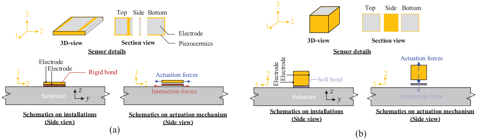
Actuating mechanisms of the traditional fixed PZT sensor and the proposed movable PZT sensor (Axes 1, 2, and 3 show the coordinates of the PZT sensor, and Axis-3 is the polarization direction of the piezoceramic sensor). (a) Traditional fixed PZT patch. (b) Proposed movable PZT sensor.

Couplant and double-sided tapes, called soft bonds in this paper, are frequently used in acoustic emission sensor calibration and accelerometer installation for short-term measurements.^27,28 They can serve as alternative bonding agents for providing mobility to the PZT sensor. However, most couplants and tapes have low viscosity, and thus good transmission can only be provided along the motion perpendicular to the contact surface.²⁶ Therefore, PZT sensors that can actuate perpendicular to the contact surface are desirable when soft bonds are used. A PZT sensor with a large thickness (i.e., rectangular parallelepiped and polarized along Axis-3) is employed as a movable sensor because it provides an adequate bonding area to actuate and sense motions perpendicular to the contact surface (along the z axis), as shown in Figure 1(b). Notable differences in actuation force directions can be observed between the fixed and movable sensors in Figure 1.

Figure 2 presents the PZT sensor and bonding materials utilized in this work. The size of the PZT sensor was 15 × 15 × 12 mm³. The electrode surfaces were along the Axis-3 direction (Figure 2(a)). Electric wires were welded to electrodes for convenient connection. One side surface without electrodes served as the contact surface. The bonding material was essentially double-sided adhesive tape (3M VHB 5608A) with a thickness of 0.8 mm (Figure 2(b)). Like a stethoscope, the PZT sensor can be easily detached from the structure after the measurement and moved to a new checkpoint for further damage detection operations, offering unprecedented flexibility in the EMI measurement.

Figure 2.

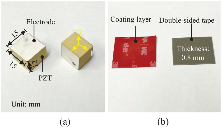
The adopted PZT sensor and bonding tape. (a) Details of the PZT sensor. (b) Details of the double-sided tape.

Corrosion-induced cracking and spalling

Concrete spalling appears in diverse geometrical shapes,²⁹ depending on the aggregates, steel spacings, and thicknesses of concrete covers.¹ Corrosion-induced concrete spalling processes can typically be divided into corrosion, delamination involving horizontal and inclined cracks, and spalling.⁸ Figure 3 presents the crack types and their development between multiple corroded rebars. The spacing of corroded steel rebars (relative to the concrete cover thickness and the diameter of the steel rebars) plays an important role in determining cracks’ propagation directions.³⁰ When the spacing is large, two inclined cracks initiate from the corroded steel rebar and propagate toward the surface, as shown by Paths 1a and 1b;³¹ meanwhile, visible surface cracks appear and propagate along Path 2. The shape of the spalled concrete cover is similar to a triangle. By contrast, when the spacing is small, the joint action of the adjacent corroded rebars can cause severe delamination (horizontal cracks along Path 3) prior to the visible surface cracking^1,32; meanwhile, other cracks propagate along Path 1a. Finally, the cracks along Paths 1a, 1b, and 3 contribute to spalling, and the shape of the spalled concrete cover is similar to a rectangle. The inclined cracks (Path 1) can be viewed as a combination of horizontal and vertical cracks.

Figure 3.

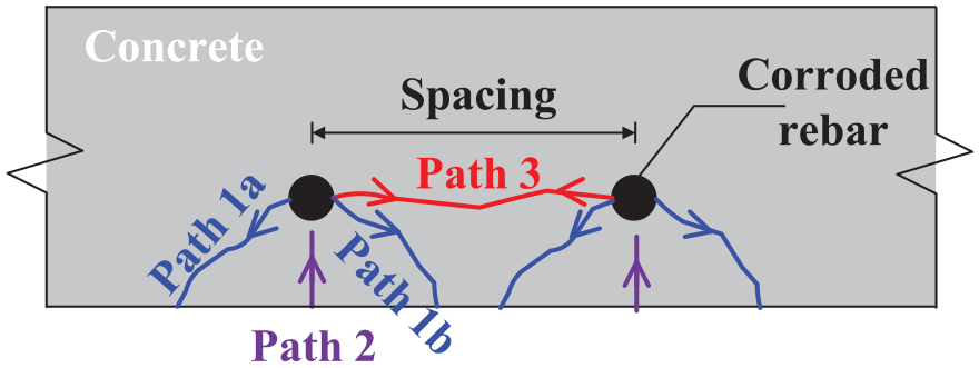
Crack types and development process of corrosion-induced spalling.

Principle of delamination detection using a movable PZT sensor

Figure 4 presents the mechanism and principle of using a movable PZT sensor to detect delamination in the cover of a concrete slab. As shown in Figure 1(b), the sensor connected to AC sweeping voltage applies actuation forces perpendicular to the contact surface (along the z axis). Only the attached sensor’s resonant frequency (denoted by f_PZT) can be easily identified in the low-frequency range when the checked area is healthy. The attached sensor’s resonance in this work differs from the sensor’s resonance tested in free-free status. Note that the resonant frequency of the PZT sensor adopted in this study is higher than 50 kHz in a free state, but the dominant resonance peak moves to around 12 kHz after being attached to the concrete surface. The low-order vibration modes of the concrete slab can hardly be captured because of the limited actuation force of the PZT sensor and the large mechanical impedance of the host structure in the frequency range below f_PZT. The strain of the PZT sensor induced by AC voltage is larger by at least one order of magnitude than the one induced by the responses of large structures, leading to low sensitivity.^33,34 Some high-order structural resonant frequencies (i.e., f_struc) can be captured with relatively low amplitude in the high-frequency range above 10 kHz.

Figure 4.

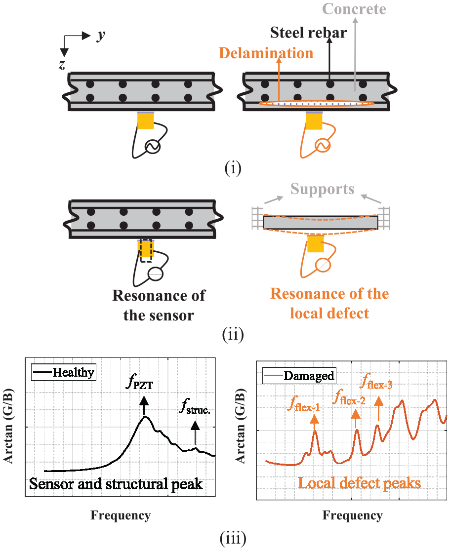
Working principle of the movable sensor for detecting the delamination of the concrete cover of a concrete slab: (i) actuation at a sweeping frequency, (ii) resonance obtained, and (iii) signal spectra.

By contrast, when the near-surface delamination occurs in a localized area, the delaminated part can be considered a two-way plate with four ends fixed or simply supported. Because of its considerably smaller size than the original slab, the local resonant vibrations of such a delaminated two-way plate can be actuated easily by the PZT sensor. Consequently, the corresponding local resonant frequencies, known as local defect resonance in composites,^35–37 can be obtained. Unlike deep delamination dominated by the thickness stretch modes, the spectral responses of near-surface delamination (i.e., shallow delamination) are dominated by flexural vibration modes,⁹ which is also proven in the numerical results in the following section. A series of resonance peaks denoted by f_flex-1, f_flex-2, and f_flex-3, corresponding to multiple flexural modes of the defect, are distinct in the low-frequency range (below f_PZT) in the measured spectra and will be used for defect assessment in this study. It is noteworthy that the frequency range of the signal spectra in Figure 4 is intentionally removed for a general expression for variable slab and delamination sizes. The specific frequency range will be discussed in the numerical and experimental cases in the following sections.

Numerical feasibility study

A series of numerical analyses were conducted to examine the feasibility of the proposed method in this section. The corresponding experimental validation is presented in the laboratory investigations.

Numerical model for simulation

As explained in Figure 3, horizontal delamination and vertical/inclined cracks play important roles in spalling induced by multiple corroded rebars. Therefore, simplified numerical models were built in consideration of the propagation of the horizontal and vertical cracks using the commercial finite element software ANSYS. Figure 5 shows the finite element model consisting of three materials: concrete, PZT, and adhesive tape materials. Steel rebars were ignored in this model, considering that they are above the delamination and have limited effects on the resonance of the delaminated layer, which was confirmed by numerical comparison. The simulated concrete slab was divided into two parts, namely, the intact and damaged parts. The damaged part was composed of five cuboid subparts. Delamination was simulated by changing the contact between the intact and damaged parts from fully bonded to unbonded interfaces. The contact interfaces were assumed to be flat for simplification, consistent with the modeling by Li et al.,³⁸ Solodov et al.,³⁶ and Kee and Gucunski.⁹ The four sides of the delaminated part are assumed as vertical interfaces perpendicular to the slab surface.

Figure 5.

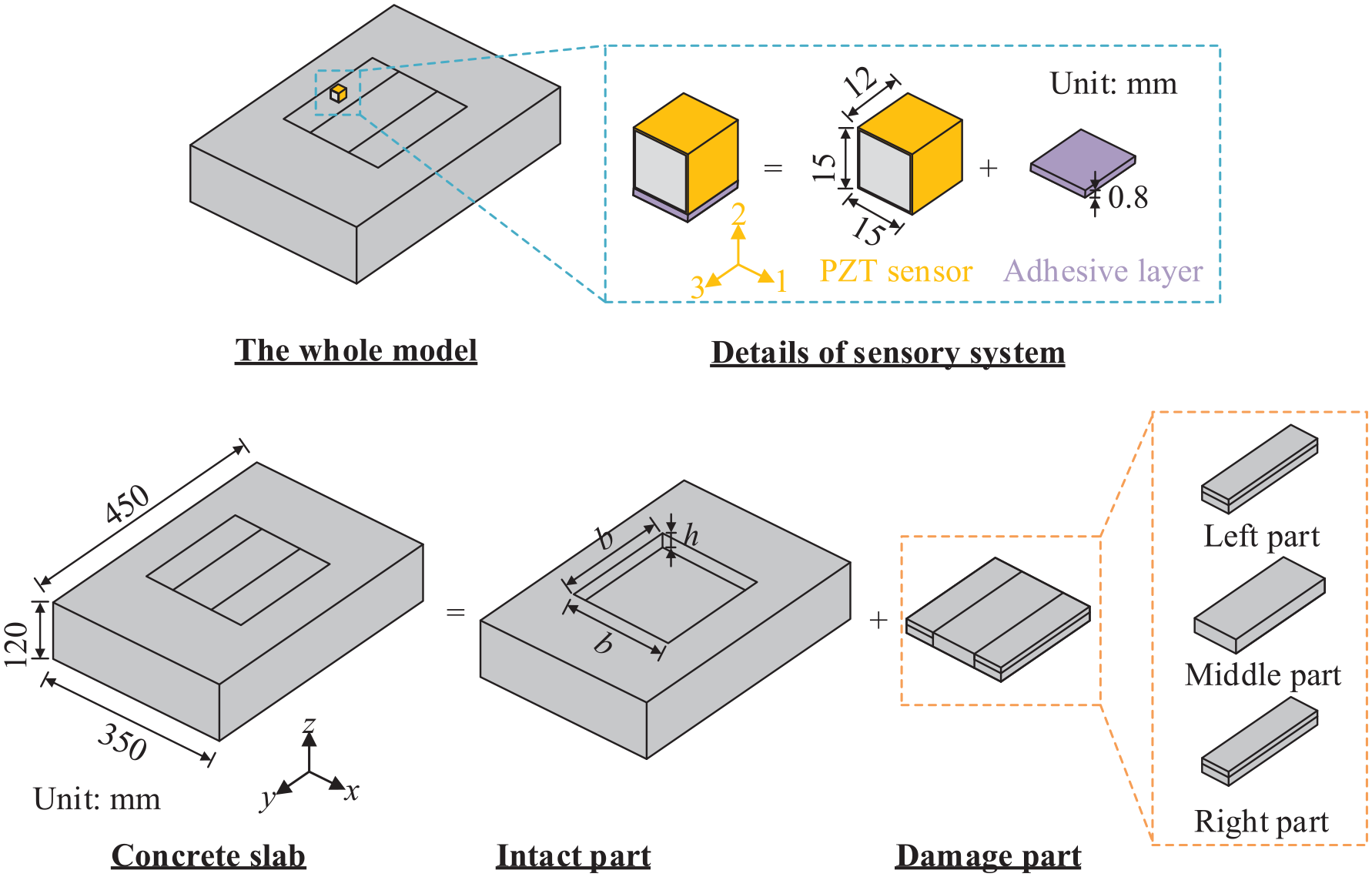
Geometric information of the numerical model.

The simulated concrete slab had the same size (length = 450 mm, width = 350 mm, and height =120 mm) as that of the tested specimen. The slab size was considerably larger than the detectable range of the sensor, indicating that the boundary conditions can be ignored. Therefore, free boundary conditions were modeled for the concrete slab. The details of the sensor are shown in Figure 2. The height of the PZT sensor (i.e., along the Axis-3 direction) was 12 mm, while the electrode area was 15 × 15 mm². The bonding layer was modeled as a thin layer having a thickness of 0.8 mm and the same area as the sensor (i.e., 15 × 12 mm²). Most of the adopted parameters are consistent with the experiment setting in the laboratory investigations.

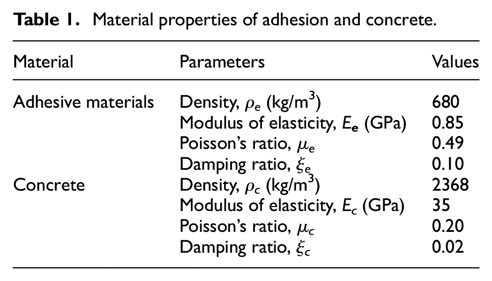
The PZT sensor was excited by a sinusoidal voltage of 1 V in the polarization directions (i.e., along the Axis-3) within a frequency range of 0–20 kHz (interval: 0.1 kHz). After a convergence analysis, element mesh sizes of 1.6 and 0.8 mm were selected for the PZT and adhesive materials, respectively; and 2.5- and 30.0-mm mesh sizes were set for the damaged and intact parts, respectively. Unlike the previous simulations in the literature, the interfaces between the PZT sensor, the adhesive layer, and the concrete are assumed to be tied only along the normal direction of the contact surface (i.e., sliding is permitted). The contact interfaces between the intact and damaged parts of the concrete are assumed to be fully bonded in a healthy status. When delamination/cracking occurs, no ties exist between two contact surfaces, and the horizontal and vertical cracks are modeled with zero thickness. Table 1 lists the material properties of the adhesion and concrete for the tested specimen in the laboratory investigation, where the former was provided by the factory and the latter was obtained from the laboratory tests. The PZT properties and element types are the same as those adopted by Sha and Zhu.¹³

Table 1.

Material properties of adhesion and concrete.

Material	Parameters	Values
Adhesive materials	Density, ρ_e (kg/m³)	680
	Modulus of elasticity, E_e (GPa)	0.85
	Poisson’s ratio, μ_e	0.49
	Damping ratio, ξ_e	0.10
Concrete	Density, ρ_c (kg/m³)	2368
	Modulus of elasticity, E_c (GPa)	35
	Poisson’s ratio, μ_c	0.20
	Damping ratio, ξ_c	0.02

Signature characteristics for different damage levels

This section correlates the signal characteristics in the EMI spectra to the different damage levels of near-surface delamination, which is a prerequisite for delamination detection. Figure 6 shows multiple damage levels that simulate the whole spalling process. The intact status is considered as the control group, where the steel spacing of b = 200 mm and the concrete cover thickness of h = 15 mm are within regular ranges. Five damage levels were simulated, where the horizontal crack width and vertical crack depth were quantified with respect to b and h, respectively (Figure 6). The label 0.25b–0.33h indicates that the horizontal cracks accounted for 25% of the steel spacing, and the vertical cracks accounted for 33% of the concrete cover thickness. Damage was considered to occur simultaneously at the two rebars. The horizontal cracks initiated from the two rebars and propagated horizontally to each other, eventually becoming one delaminated layer. Meanwhile, the vertical cracks were assumed to occur and propagate on three sides simultaneously. The simulated damage development was consistent with the cracking process shown in Figure 3 and that reported by Zhang and Su.³⁹ The sensor was installed on a fixed checkpoint (i.e., x = −3b/8 and y = 0) on the bottom surface of the left delaminated area.

Figure 6.

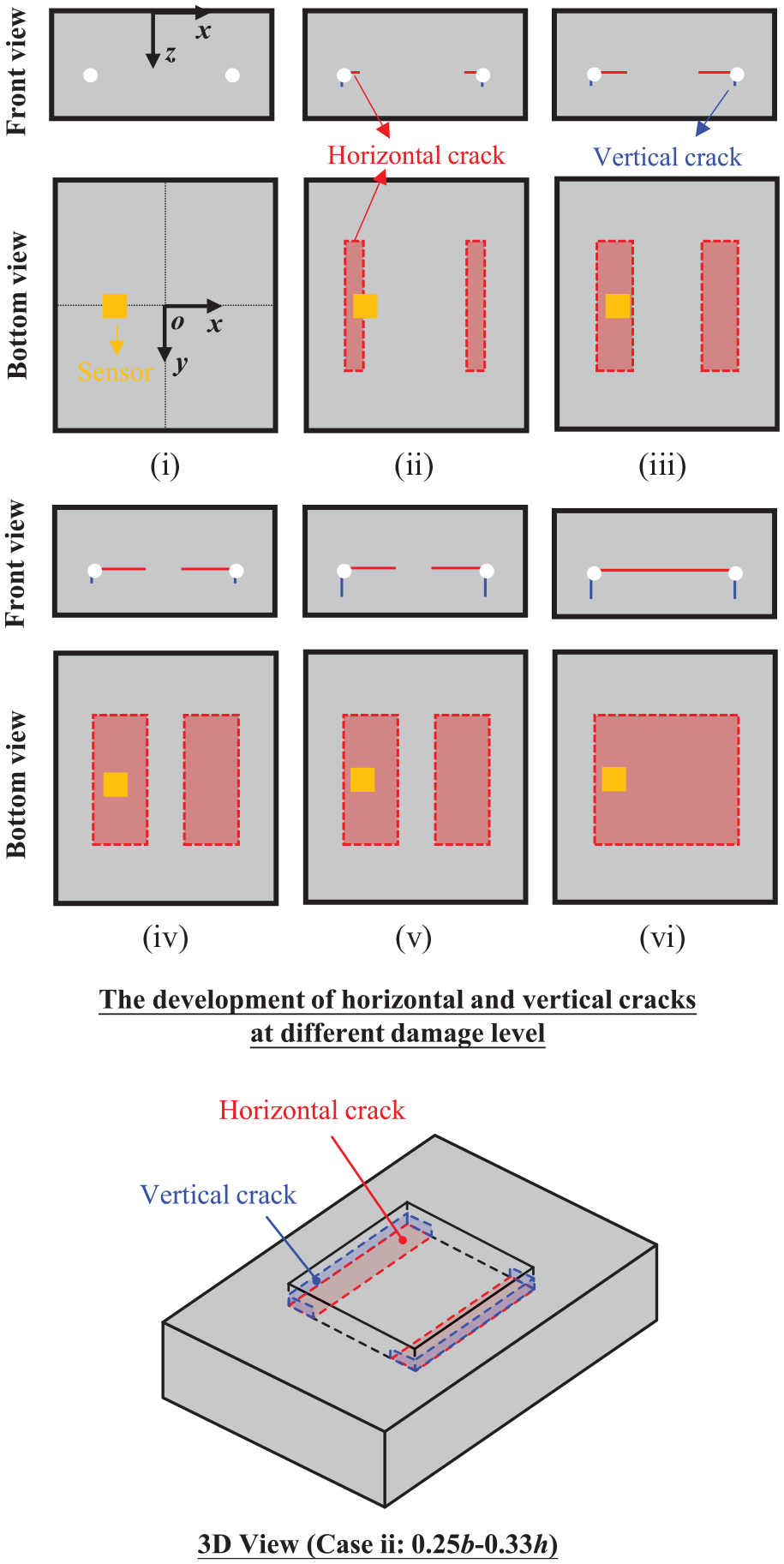
Different damage levels for simulating the spalling process: (i) intact, (ii) 0.25b–0.33h, (iii) 0.50b–0.33h, (iv) 0.75b–0.33h, (v) 0.75b–0.66h, and (vi) 1.00b–0.66h.

Figure 7 presents the signal spectra at different damage levels. The dimensionless physical quantity G/B stands for the complementary angle of the phase, and it has been proven effective in capturing resonance peaks in the EMI spectra,¹³ where G and B refer to the conductance (i.e., the real part of admittance) and susceptance (i.e., the imaginary part of admittance) of the signal, respectively. The obtained frequency spectra were smoothed via a moving average operation with a 500-Hz window to remove minor peaks that were caused by measurement noise and did not correspond to resonance peaks, thereby facilitating peak identification. Figure 8 shows the vibration mode shapes corresponding to several important peaks. The vibration modes in Figures 7 and 8 are categorized into three types, namely, the PZT mode, slab modes (i.e., related to the behavior of the slab), and local defect modes according to their deformation type, which are labeled as PM, SM, and LDM, respectively. Several researchers discussed the definitions of the PZT mode and structural modes.^13,21,25 In EMI techniques, the PZT mode exhibits a distinct amplitude, while the structural modes usually have relatively smaller amplitudes.²¹ The local defect modes have been widely discussed in composite materials. The captured local defect modes present larger amplitudes than structural modes in the spectrum and can be utilized for delamination and debonding detection.^11,17,18

Figure 7.

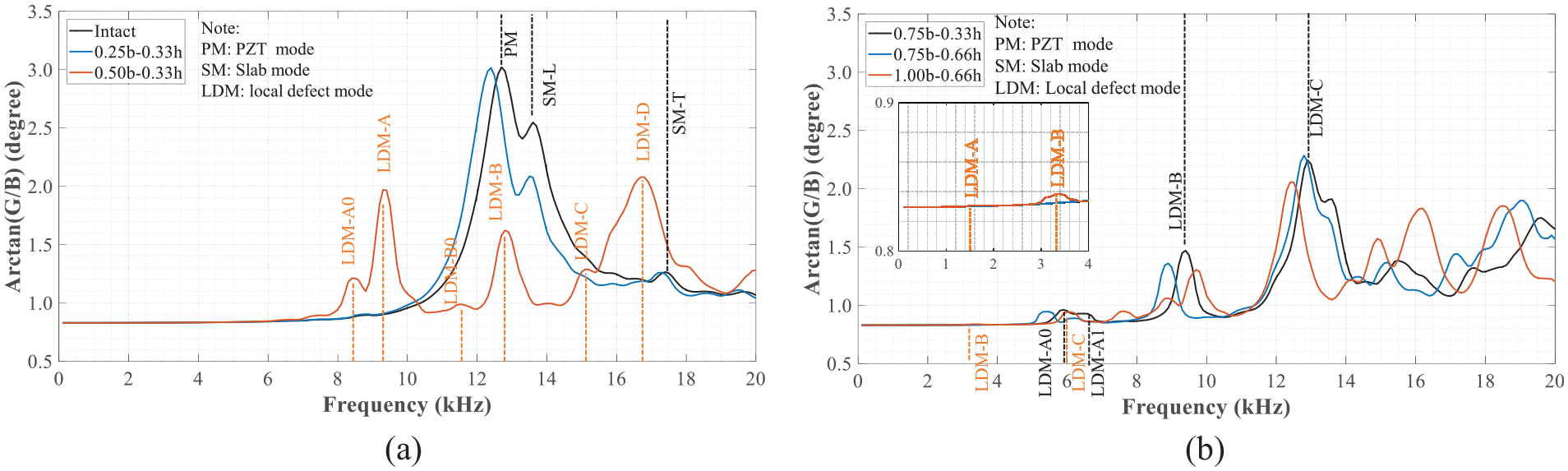
Signal spectra at different damage levels: (a) cases i–iii and (b) cases iv–vi.

Figure 8.

Classic vibration mode shapes corresponding to the characteristic peaks in the spectra (the color shows the displacement magnitude. The minimum and maximum displacements are shown in blue and red, respectively, and the intermediate displacements are shown in green and yellow). (a) Mode shapes of the PZT sensor and slab (Case i: intact). (b) First four captured local defect modes (Case iii: 0.50b–0.33h).

Figure 7(a) shows the signal spectra at the early stage of the spalling process. In Cases (i)–(iii), the sensor was located above the intact area, the boundary of the intact and delaminated areas, and the delaminated area, respectively. In the intact case (Case i), three peaks in the spectrum were labeled as PM (f_PZT = 12.7 kHz), SM-L (13.6 kHz), and SM-T (17.4 kHz), whose corresponding mode shapes are shown in Figure 8(a). The peak PM corresponded to the attached PZT sensor mode, whose displacements were concentrated on the sensor and bonding layer. Consequently, the peak PM was highly dependent on the properties of the sensor and the adhesive layer. The peak SM-L (where L indicates that the sensor is on the left side) corresponded to a high-order concrete slab mode excited by the PZT sensor. Its vibration displacements mainly occurred on the sensor and at the edge of the slab. The peak SM-T corresponded to the thickness stretch mode of the concrete slab, which was governed by the thickness and properties of the concrete slab. In the intact case, no peaks were found in the low-frequency ranges (i.e., <f_PZT).

In Case ii (i.e., 0.25b–0.33h), the signal spectrum retained a similar pattern with the intact case. The peak PM moved leftward, and the peak SM-L retained nearly the same frequency. The peak SM-T showed a slight change due to the changes in the local boundary conditions. In the third case (i.e., 0.50b–0.33h), the pattern of the signal spectrum changed considerably compared with those in the previous two cases. The sensor modes (PM) and two identified slab modes (SM-L and SM-T) were no longer captured. A series of peaks highly related to the local defect appeared in the signal spectrum. Six easily observed peaks are labeled as the local defect mode in Figure 7(a), and their mode shapes are shown in Figure 8(b). The first two peaks (LDM-A0 and LDM-A) corresponded to the first-order local defect mode, in which the major deformation was along the length of the delaminated layer. The first-order mode was split into two because of the simultaneous delamination appearance on the left and right sides. The peak LDM-A0 (8.5 kHz) showed the deformation of two delaminated areas on the left and right sides, while LDM-A (9.4 kHz) showed the mode only related to the left delaminated area. Similar phenomena were observed for the peaks LDM-B0 (11.6 kHz) and LDM-B (12.8 kHz), both of which corresponded to the third-order mode along the length of the delaminated layer. The second-order mode was missing because the PZT sensor was installed on the symmetric plane. The peaks LDM-C (15.1 kHz) corresponded to the first-order mode along the width of the delaminated layer, and LDM-D (16.9 kHz) corresponded to the fifth-order modes along the length of the delaminated layer.

Figure 7(b) plots the signal spectra at the further development stage of the spalling process. The horizontal and vertical cracks continued to propagate in the three cases. By comparing Case iv (0.75b–0.33h) with Case iii (0.50b–0.33h) and Case v (0.75b–0.66h), the effects of the horizontal and vertical cracks could be observed, respectively. In Case iv (0.75b–0.33h), the local defect modes moved leftward compared with those in Case iii (0.50b–0.33h), but the signal spectrum had the same pattern. LDM-A0 and LDM-A moved from 8.5 and 9.4 kHz to 5.9 and 6.6 kHz, respectively. The peak LDM-B0 became too weak to capture. The peaks LDM-C and LDM-D moved from 15.1 and 16.9 kHz to 9.4 and 12.9 kHz, respectively. The signal spectrum in Case v (0.75b–0.66h) also had the same pattern as that in Case iv (0.75b–0.33h). However, the leftward movement of the local defect modes induced by the vertical crack development was much smaller than that caused by the horizontal cracks. For example, LDM-A0 and LDM-A moved to 5.5 and 6.3 kHz, respectively, with only 0.4 and 0.3 kHz differences, respectively. Aside from the frequency movement, the peaks’ magnitude also decreased as the horizontal and vertical cracks propagated.

In Case vi (1.00b–0.66h), the two horizontal cracks merged, leading to a dramatic change in the detected region compared with the two other cases. The first several local defect modes moved leftward substantially. However, the peak LDM-A was too weak to be captured. The PZT sensors typically have low sensitivity in the low-frequency range because of the high impedance of the capacitance-type sensor in this range, which prevents the generated charge from being retained and results in underestimated structure responses.⁴⁰ For the adopted PZT sensor in this study, a frequency range smaller than 2 kHz is not recommended when using the EMI technique in practice. Although the first-order local defect mode was missed, high-order local defect modes can still be captured in the signal spectrum.

Effect of bonding layer

Sha and Zhu¹³ numerically and experimentally showed that the resonant frequencies of concrete cubes captured by the EMI technique do not vary with the properties of the rigid adhesive layer (e.g., epoxy). However, the movable sensors used double-sided tape as the bonding material, which was considerably different from the traditional rigid bonding layers. Considering its weak bonding along the tangential direction of the contact surface, the effect of the flexible bonding layer is examined to show the generalizability of the proposed method.

Large bonding thicknesses and high surface unevenness may affect through-transmission characteristics and reduce sensor sensitivity.^13,26,41 In particular, using tape bonding can hardly ensure a perfect contact surface in practical measurement. Such undesirable weak bonding was simulated by reducing the modulus of elasticity of the bonding layer.

Figure 9 shows the effect of the modulus of elasticity (E_e) of the bonding layer on the signals in the intact and damaged cases (i.e., Case i and Case iv: 0.75b–0.33h). The peak PM (corresponding to the PZT sensor mode) in the intact case was substantially affected by three E_e values (namely, 0.50, 0.85, and 1.20 GPa) in the signal spectrum (Figure 9(a)). As E_e increased, the PZT peaks moved rightward (from 10.6 to 14.6 kHz) and upward (from 1.5° to 3.8°), indicating the higher transmission ability of the bonding layer. As the transmission ability increased, the resonance peaks of the slab (i.e., SM-L and SM-T) were strengthened and could easily be identified, but the frequencies of the two slab modes varied slightly.

Figure 9.

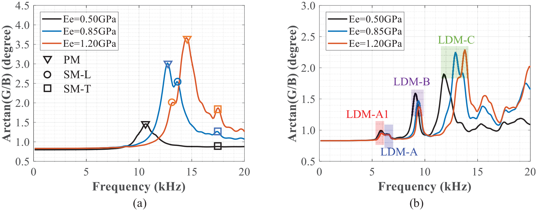
Effect of the modulus of elasticity of the bonding layer: (a) intact case (Case i) and (b) damaged case(Case iv: 0.75b–0.33h).

In the damaged case (Case iv: 0.75b–0.33h) shown in Figure 9(b), as E_e increased, the frequencies of the first two local defect modes remained the same, while their magnitude showed a slight variation. But the frequencies of the high-order local defect modes slightly increased with increments in E_e. For example, the frequencies of LDM-B and LDM-C increased from 9.1 to 9.5 kHz and from 11.8 to 13.8 kHz, respectively. The likely reasons for the frequency increments of the local defect modes were: (1) the sizes of the PZT sensor and bonding layer were not ignorable compared with the delaminated area and (2) the resonant frequency of the PZT sensor shown in Figure 9(a) also fell in this frequency range and produced the disturbance to the local defect modes. Although decreasing the size of the PZT sensor could reduce the frequency shifting of the local defect modes, it may not be an ideal solution considering the associated weak signal amplitudes.²¹ Given that the study’s goal is to detect near-surface delamination in concrete structures, an approximate evaluation can be accepted.

In summary, the variation in the bonding layer considerably affected the sensor peak but only slightly influenced the structural peaks and the fundamental local resonant peak. It is noteworthy that the modulus of elasticity of the concrete also affected the frequency and amplitude of the sensor mode PM, but the effect was not as remarkable as that of the bonding layer.

Effects of slab size and boundary conditions

Figure 10 shows the effects of varying the area and boundary condition of the slab on the intact and damaged cases. In the intact case (i.e., Case i), the signal spectrum became increasingly smooth as the slab area increased (Figure 10(a)). Meanwhile, mode SM-L disappeared, whereas SM-T could still be captured, because the former and latter were sensitive to the slab area and thickness, respectively. When the boundary conditions changed from free to fixed, the SM-T frequencies still varied slightly. Similarly, the frequency of the PZT peak (i.e., PM) varies slightly with different areas and boundary conditions, as the sensor area was considerably smaller than the slab area. In the damaged case (i.e., Case iv: 0.75b–0.33h), the three labeled peaks exhibited smaller variations as the slab area and boundary conditions changed compared with those changes in terms of the bonding layer (Figure 10(b)). In general, the slab sizes and boundary conditions exerted limited effects on the signal spectra, implying that the obtained findings could be directly extended to slabs of larger sizes.

Figure 10.

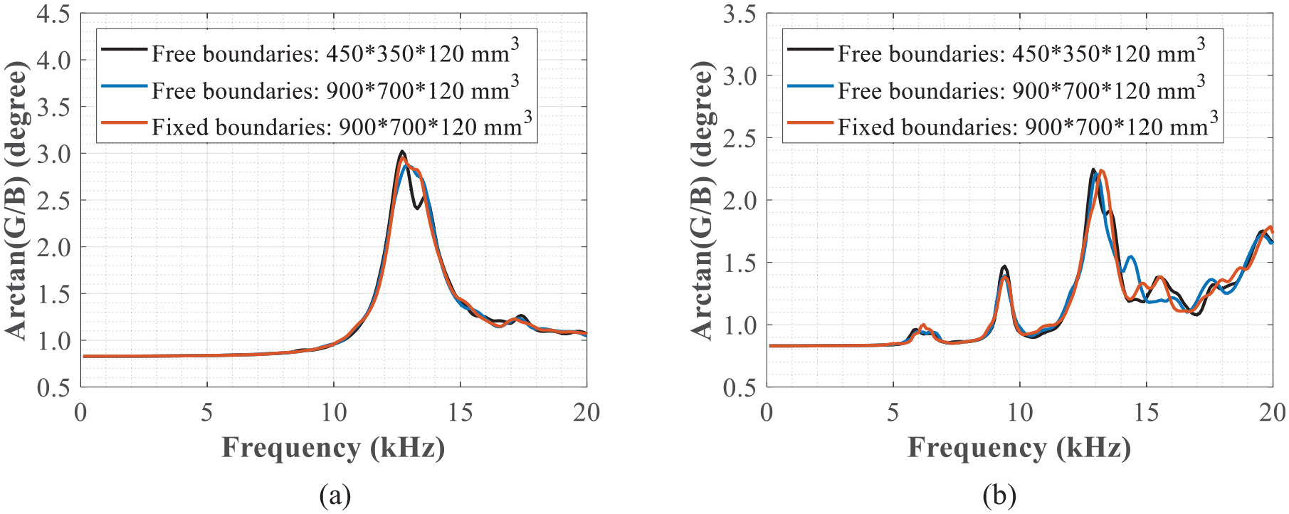
Effect of the area size and boundary conditions of the concrete slab: (a) intact case (Case i) and (b) damaged case(Case iv: 0.75b–0.33h).

Quantitative analyses of local defect modes

Although the first-order local defect mode is insensitive to the bonding layers, the slab size, and the slab boundary condition, it is still affected by multiple properties of the near-surface defect, such as delamination size (i.e., length of the horizontal and vertical cracks), shape, and boundary conditions. Therefore, the evaluation of defect size based on the local defect resonance frequency is still challenging. Flat-bottomed delamination with no vertical cracks was often simulated in composite structures.^36,42 Solodov et al.²⁹ presented an equation to calculate the first-order resonant frequency of a rectangular defect with a flat bottom in a composite structure, in which the boundary conditions were simply assumed to be fixed (i.e., no rotation). The equation cannot be directly applied to near-surface concrete defects with complicated boundary conditions.

Kee and Gucunski⁹ categorized the boundary conditions of flat-bottomed square delaminated plates with width a and thickness h (without vertical cracks) into three types: (a) fully clamped boundary conditions are suitable for very shallow delamination (a/h > 20); (b) for delamination with 5 < a/h ≤ 20, the boundary conditions are in between simply supported and fully clamped conditions; and (c) the boundary conditions are weaker than simply supported conditions for a/h ≤ 5. The differences arise from varying edge constraining effects. The analytical expression for the first-order resonant frequency of the flat-bottomed square defects, regressed from numerical simulation data by Kee and Gucunski,⁹ is

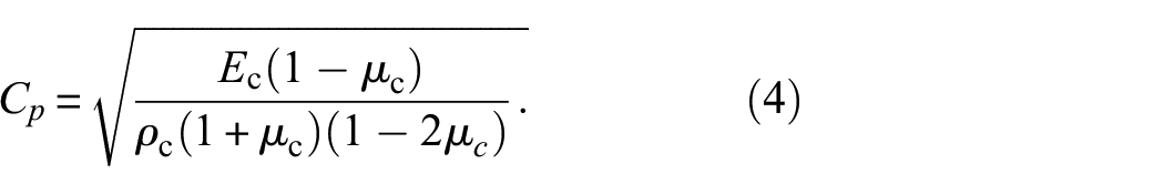
f_{1} = ε β_{1} \frac{C_{p}}{h} {(\frac{h}{a})}^{2} = ε \frac{1}{h} {(\frac{h}{a})}^{2} \cdot β_{1} C_{p}

(1)

where h and a are the thickness and fictitious width of the delaminated part, respectively; ε stands for the correction factor for the edge effects, as shown in Equation (2); β₁ is the correction factor for Poisson’s ratio μ_c, as shown in Equation (3); C_p denotes the compressive wave velocity, as shown in Equation (4),

ε = 1.64 e^{0.0014 (a / h)} - 1.812 e^{- 0.22 (a / h)}

(2)

β_{1} = \frac{π \sqrt{(1 - 2 μ_{c})}}{\sqrt{12 {(1 - μ_{c})}^{2}}}

(3)

C_{p} = \sqrt{\frac{E_{c} (1 - μ_{c})}{ρ_{c} (1 + μ_{c}) (1 - 2 μ_{c})} .}

(4)

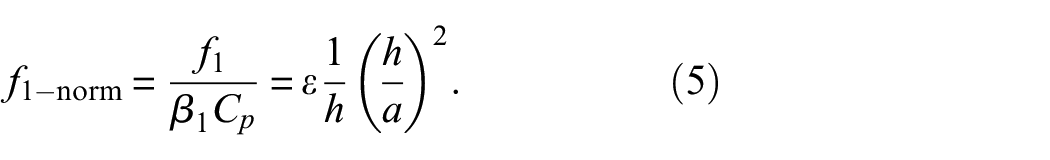
By removing the effect of material properties, the normalized first-order resonant frequency f_1-norm is obtained for generalization as follows:

f_{1 - norm} = \frac{f_{1}}{β_{1} C_{p}} = ε \frac{1}{h} {(\frac{h}{a})}^{2} .

(5)

If the defect is a rectangle, the rectangular shape can be converted to a square shape with an equivalent edge dimension,⁹ as shown in Equation (6):

a = \frac{\sqrt{2} a_{w} a_{l}}{\sqrt{a_{w}^{2} + {a_{l}}^{2}}}

(6)

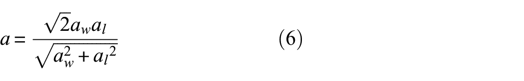
where a_w and a_l stand for the width and length (a_l > a_w) of the rectangular delamination, respectively. For a long rectangle (a_l/a_w > 3), a converges to $\sqrt{2}$ a_w, indicating that the smaller width dominates the first-order defect resonant frequency. Considering that actual delaminated shapes may be unknown, a/ $\sqrt{2}$ can be approximately considered the lower bound of the delamination dimension, and a² can be considered the lower bound of the delamination area.

The concrete material properties in Equation (4) may not be available in practice. Then, the compressive wave velocity C_p can be estimated from

f_{thickness} = \frac{β_{2}}{2 T} C_{p}

(7)

where T is the slab thickness, and β₂ is the correction shape factor that depends on the Poisson’s ratio of the concrete. The values of 0.96 and 0.2 are recommended for β₂ and μ_c, respectively.⁴³

Table 2 compares the normalized first-order local resonant frequencies of a square defect obtained from the modal analyses of finite element models with the analytical expressions proposed by Kee and Gucunski.⁹ The delaminated layer thickness (h) was from 10 to 30 mm, covering the common range of concrete covers. The defect width (a) was from 100 to 200 mm, covering the normal steel rebar spacing in concrete structures. The simulated slab had a size of 1000 × 1000 × 120 mm³ with the boundaries clamped to represent a general situation. Notably, the correction factor in Equation (2) does not consider vertical cracks, corresponding to the damage case 1.00a–0.00h defined in this study. But in the finite element models, two damage cases, namely, 1.00a–0.00h and 1.00a–0.75h, were simulated.

Table 2.

The normalized first local defect resonance of a square defect.

Defect size		f _1-norm simulation		f _1-norm by Equation (5)
a (m)	h (m)	1.00a–0.00h	1.00a–0.75h	1.00a–0.00h	Error (%)
0.100	0.010	1.436	1.188	1.462	1.9
0.125	0.010	1.011	0.790	0.994	−1.7
0.150	0.010	0.719	0.569	0.715	−0.5
0.175	0.010	0.536	0.416	0.536	0.0
0.200	0.010	0.421	0.303	0.416	−1.2
0.100	0.015	2.054	1.602	1.856	−9.6
0.125	0.015	1.376	1.084	1.315	−4.5
0.150	0.015	1.010	0.768	0.975	−3.5
0.175	0.015	0.755	0.556	0.748	−0.9
0.200	0.015	0.585	0.442	0.590	1.0
0.100	0.020	2.486	1.910	2.097	−15.6
0.125	0.020	1.682	1.354	1.531	−9.0
0.150	0.020	1.201	0.992	1.164	−3.1
0.175	0.020	0.973	0.721	0.912	−6.4
0.200	0.020	0.748	0.535	0.731	−2.3
0.100	0.025	2.604	1.978	2.244	−13.8
0.125	0.025	1.917	1.566	1.677	−12.5
0.150	0.025	1.397	1.106	1.300	−7.0
0.175	0.025	1.113	0.780	1.035	−7.0
0.200	0.025	0.930	0.695	0.842	−9.5
0.100	0.030	2.710	2.009	2.332	−13.9
0.125	0.030	1.998	1.639	1.776	−11.1
0.150	0.030	1.616	1.175	1.398	−13.5
0.175	0.030	1.207	0.995	1.128	−6.6
0.200	0.030	1.028	0.739	0.928	−9.7
Mean value					−6.4
Standard deviation					5.3

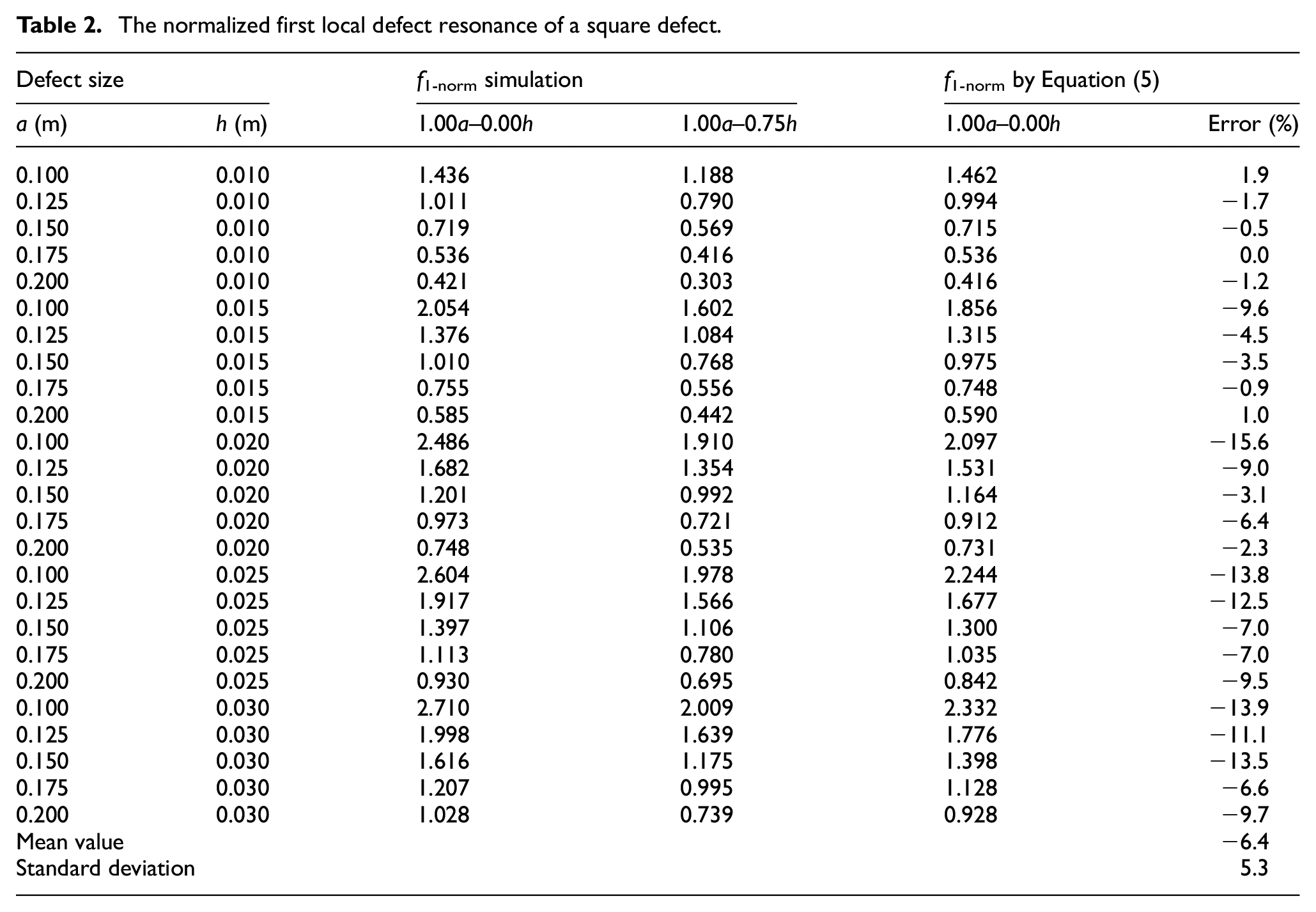
In the damage case 1.00a–0.00h, the mean and maximum errors between the simulation and the prediction of Equation (5) were −6.4% and −15.6%, respectively, indicating a fair accuracy of Equation (5). Meanwhile, Equation (5) could not accurately predict the damage case 1.00a–0.75h because the existence of the vertical cracks reduced resonant frequencies apparently.

Therefore, Equations (8) and (9) are regressed from the simulation results in Table 2 to estimate the fictitious width of the delamination part in a square shape, in which the units of defect size and frequency are meter and hertz, respectively. Considering vertical cracks with 1.00h lead to the falling of spalled concrete, the cases with 0.00h and 0.75h are considered as the bounds of the vertical crack depths in practice. The estimated width (a) corresponding to 0.00h and 0.75h are considered the upper and lower bounds of such width, respectively. If the delaminated area is a long rectangular shape, a_w can be estimated by a/ $\sqrt{2}$ , as suggested by Equation (6),

\begin{matrix} a = 0.1892 - 0.1298 f_{1 - norm} + 5.873 h + 0.03583 {f_{1 - norm}}^{2} \\ - 2.123 f_{1 - norm} h; for the upper bound; R^{2} = 0.98 \end{matrix}

(8)

\begin{matrix} a = 0.1902 - 0.1515 f_{1 - norm} + 4.892 h + 0.04918 {f_{1 - norm}}^{2} \\ - 2.054 f_{1 - norm} h; for the lower bound; R^{2} = 0.98 . \end{matrix}

To sum up, the proposed delamination detection method could be implemented as follows:

(a)The PZT sensor was attached to a checkpoint on the target surface by using double-sided tape.

(b)The EMI signal spectrum was recorded from 1 to 20 kHz, and a moving average operation with a 500-Hz span might be applied if necessary.

(c)The signal spectral pattern was assessed to determine whether delamination existed or not. If only a distinct peak was found in the frequency range of 10–15 kHz, the checkpoint was considered healthy. If multiple peaks were found in the 1–15 kHz range and the first peak appeared below 10 kHz, the checkpoint was considered delaminated.

(d)The delaminated area was estimated by substituting the first resonant frequency into Equations (6), (8), and (9), if delamination was detected.

(e)The sensor was subsequently detached, and detection was repeated at a new checkpoint by using the same sensor.

It should be pointed out that the quantification of defect sizes is rather approximate and only for quick reference. In practice, complex boundary conditions (e.g., numerous closely distributed delaminated zones) and geometric shapes may present multiple peaks in the target frequency range and complicate peak identification. Interpreting peaks is an essential and highly specialized process that requires profound professional knowledge. Emerging tools, such as machine learning and artificial intelligence methods, may greatly facilitate and improve the interpretation of multiple peaks in the spectra,^44,45 which will be explored in the future.

In addition, the sensor size and adhesive materials can be further optimized to improve the capability of peak identification and achieve high sensitivity.¹³ To avoid any undetectable defects, the distance interval between every two checkpoints is recommended to be not more than 200 mm.

Laboratory experimental validations

Artificial delamination (i.e., flat delamination cracks parallel to the surface) was introduced in most previous detection studies. Although this introduction facilitated the comparison with the analytical and numerical results, it hindered the understanding of the development process of delamination; additionally, many cracks in concrete slabs are wavy with variable depths.⁹ Therefore, the experimental validations in this section simulated a real spalling process induced by steel rebar corrosion. The proposed method in the numerical part was used to detect the delamination, and the evaluation results were verified by cutting the tested concrete slab.

Experimental setup and procedure

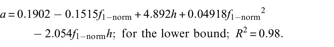
Figure 11 presents the geometry of the specimen and the details of the steel rebars. The cast concrete slab had a size of 450 × 350 × 120 mm³, which was identical to that in the numerical model. The rectangular concrete slab was reinforced by two steel rebars (HRB 400), which had a diameter of 10 mm and a center-to-center spacing of 100 mm. The length of each steel rebar was 550 mm to allow for an electrical connection. The actual corroded length was only 300 mm. The ends of the steel rebars in the slab were coated with epoxy to prevent corrosion and avoid spalling in large areas, as this study mainly focused on the early detection of small-size spalling. Given the limitation in installation precision, the concrete cover thickness was equal to 15 and 20 mm, respectively, for the left (labeled as L) and right (labeled as R) steel rebars.

Figure 11.

Geometry of the slab specimen and details of the steel rebars.

A batch of concrete specimens was cast for measurement, including four 150-mm cubes and one slab. The cubes were used to measure the modulus of elasticity and compressive strength, where the former was measured by the EMI technique,¹³ and the latter was obtained through uniaxial compressive testing. The mix proportions and measured material properties of concrete are summarized in Table 3. To facilitate corrosion, 4% NaCl by weight of cement was added to the concrete mix. The specimen was demolded after 24 h and was cured in an air-dry condition for 28 days before the corrosion tests.

Table 3.

Material proportions of the adopted concrete materials.

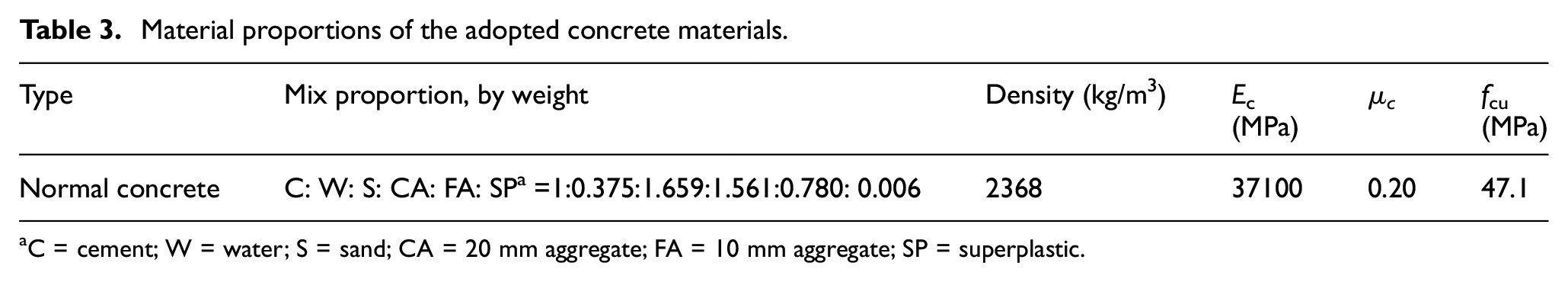
Type	Mix proportion, by weight	Density (kg/m³)	E _c (MPa)	μ_c	f _cu (MPa)
Normal concrete	C: W: S: CA: FA: SP^a =1:0.375:1.659:1.561:0.780: 0.006	2368	37100	0.20	47.1

^aC = cement; W = water; S = sand; CA = 20 mm aggregate; FA = 10 mm aggregate; SP = superplastic.

Accelerated corrosion techniques were employed to considerably reduce the duration of the corrosion period. Figure 12 presents the experimental setup for the accelerated corrosion tests and damage detection using the EMI technique. The wetting-drying cycle process was used. Figure 12(a) shows the wetting stage, in which a wet sponge containing a 5% NaCl solution (serving as the electrolyte) covered the top slab surface with a stainless steel mesh (serving as the cathode). Each steel rebar was connected to one DC power source and applied with constant current. Table 4 presents the corrosion procedure and the duration of each step, where corrosion duration refers to the duration of the electric current being applied. In the first 60-h corrosion time, the current intensity was 500 μA/cm². Then, the current density was increased to 750 μA/cm² in the rest of the corrosion procedure. Large damage might be produced because of the absence of a dissipation period for the radial pressure exerted at the steel/concrete interface.^46,47 Considering that the goal of this experiment was to validate the effectiveness of the proposed delamination detection instead of predicting the corrosion procedure, high current densities are regarded as acceptable.

Figure 12.

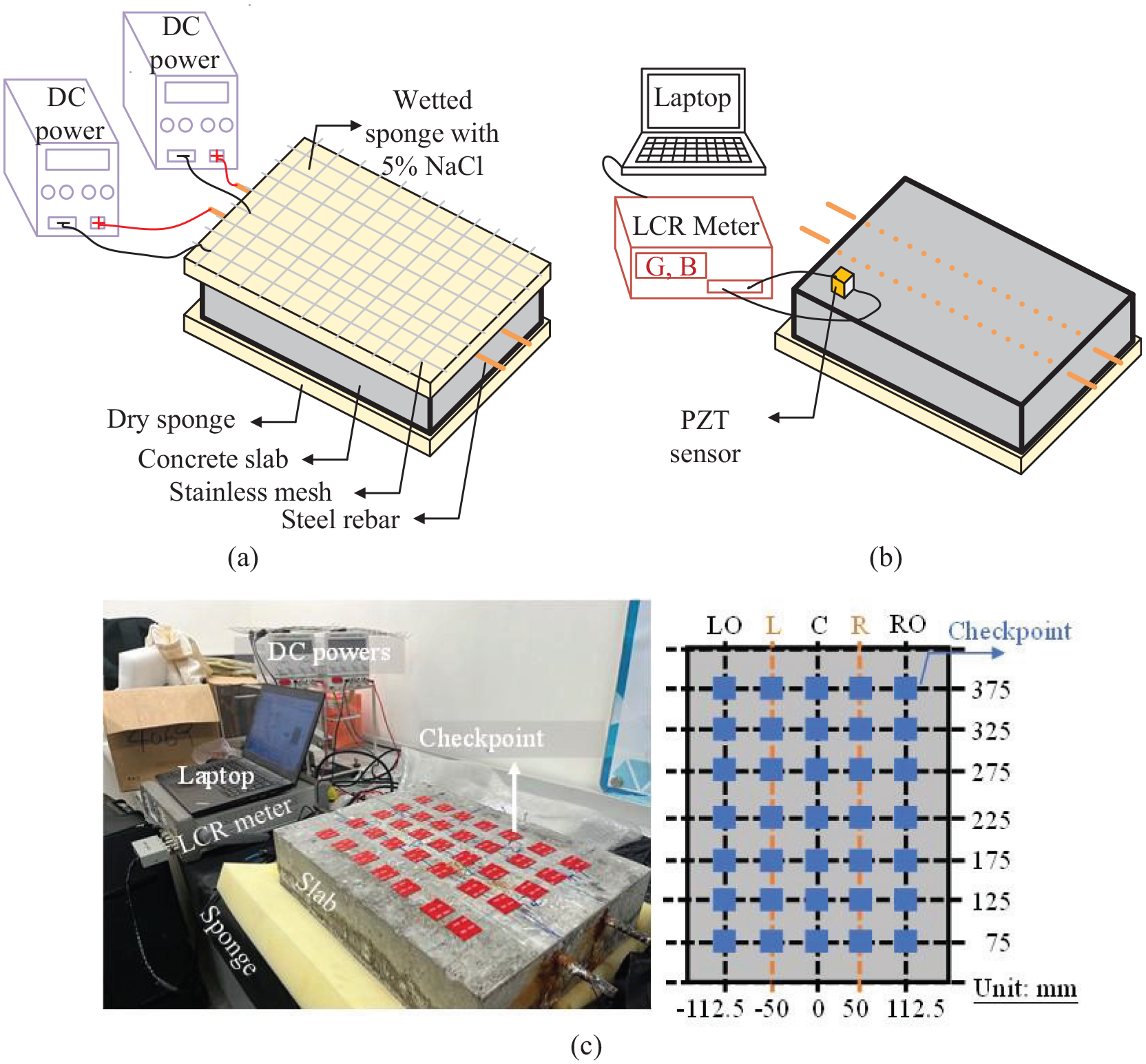
Experimental setup for the accelerated corrosion tests and delamination detection using the EMI technique: (a) wetting: accelerated corrosion tests, (b) drying: damage detection, and (c) experimental photo and checkpoints.

Table 4.

Corrosion time procedure at the wetting stage.

Step	Duration of eachstep for inducedcorrosion (hours)	Currentdensity(μA/cm²)	Accumulatedcorrosiontime (hours)
1	0	0	0
2	60	500	60
3	48	750	108
4	72	750	180
5	Before cutting: thetested slab wasplaced in a dry conditionin the laboratoryfor 6 months

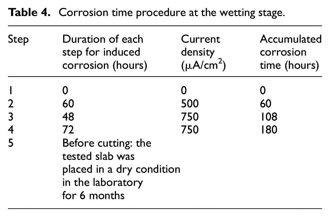
Figure 12(b) shows the damage detection conducted during the dry stage with no current being applied, wherein only one sensor was attached to multiple checkpoints on the concrete slab for measurement. The sensor type and bonding tape were similar to those in Figure 2. When one measurement was finished, the sensor was detached from the old checkpoint and attached to a new checkpoint by using the double-sided tape. The PZT sensor was excited with an AC voltage of 1 V, and the EMI spectra were measured by the LCR device (Keysight E4980AL) connected to a laptop. The frequency ranges and intervals were from 2 to 20 kHz and 25 Hz, respectively. The room temperature and humidity during measurement were around 20°C and R.H. 60%, respectively.

Figure 12(c) shows the experimental photo and the layout of checkpoints. The checkpoints were categorized into three groups according to their locations relative to the steel rebars, namely, between the steel rebars (i.e., Axis C), on the steel rebars (i.e., Axes L and R), and outside the steel rebars (i.e., Axes LO and RO). The center-to-center distance between the checkpoints was 50 mm, which made the checkpoints dense enough to examine the slab carefully. Checkpoint L75 refers to a point located on Axis L and 75 mm away from the bottom side of the slab.

Table 4 mentions the status “before cutting,” which happened about 6 months after Step 4. Considering that the 6-month period and multiple times of transportation might have caused new damage, the delamination detection was conducted again as Step 5, aiming to correlate the final detection results to the cutting results of the slab.

Damage detection

Figure 13 presents the typical signal spectra recorded after 0 and 60 h of corrosion. At this stage, no damage was visible on the concrete surface. The signal patterns at different checkpoints were similar, but the distinct peaks varied from 11.0 to 13.2 kHz because of the different surface unevenness at these points. The peaks of the PZT sensor modes were within the frequency range mentioned in the numerical part, indicating the rationality of the modulus of elasticity of the double-sided tape assumed in numerical analyses. Meanwhile, the SM-L and SM-T modes could be captured. Slight variations in the frequencies of SM-L and SM-T modes are likely caused by the nonhomogeneous and nonuniform thickness of the concrete slab.

Figure 13.

Signals comparison after 0 and 60 corrosion hours measured at different locations: (a) 0 h and (b) 60 h.

Figure 14 presents the visual inspection of the concrete slab over time. No visible cracks were observed in the first two steps. After a 108-h corrosion process (i.e., Step 3), two different damage types were observed on the slab surface (Figure 14(a)). The surface damage did not expand after the 180-h corrosion time (i.e., Step 4). Figure 14(b) presents the details of the damage that occurred after 108-h corrosion time. An extended surface crack appeared above the rebar on the right side. In addition, a 130-mm-long and 30-mm-wide approximately elliptical spalling area occurred at a shallow depth (around 4 mm) between Axes L and R and between Axes 225 and 375. The spalling of the superficial damage was caused by salt crystallization, a type of physical damage that occurs frequently during the wetting-drying cycle.⁴⁸ The damage is caused by internal stress arising from the formation of salt crystals in concrete when the pore solution becomes supersaturated. Given the skin effect of concrete, the maximum chloride concentration usually occurs in a shallow depth (i.e., ∼3 mm) during the wetting-drying cycle.⁴⁹ In this study, a continuous surface crack with a width of ∼0.05 mm was observed at the location of the R-rebar. The following discussions employed the checkpoints on Axes 175 and 275 for comparison.

Figure 14.

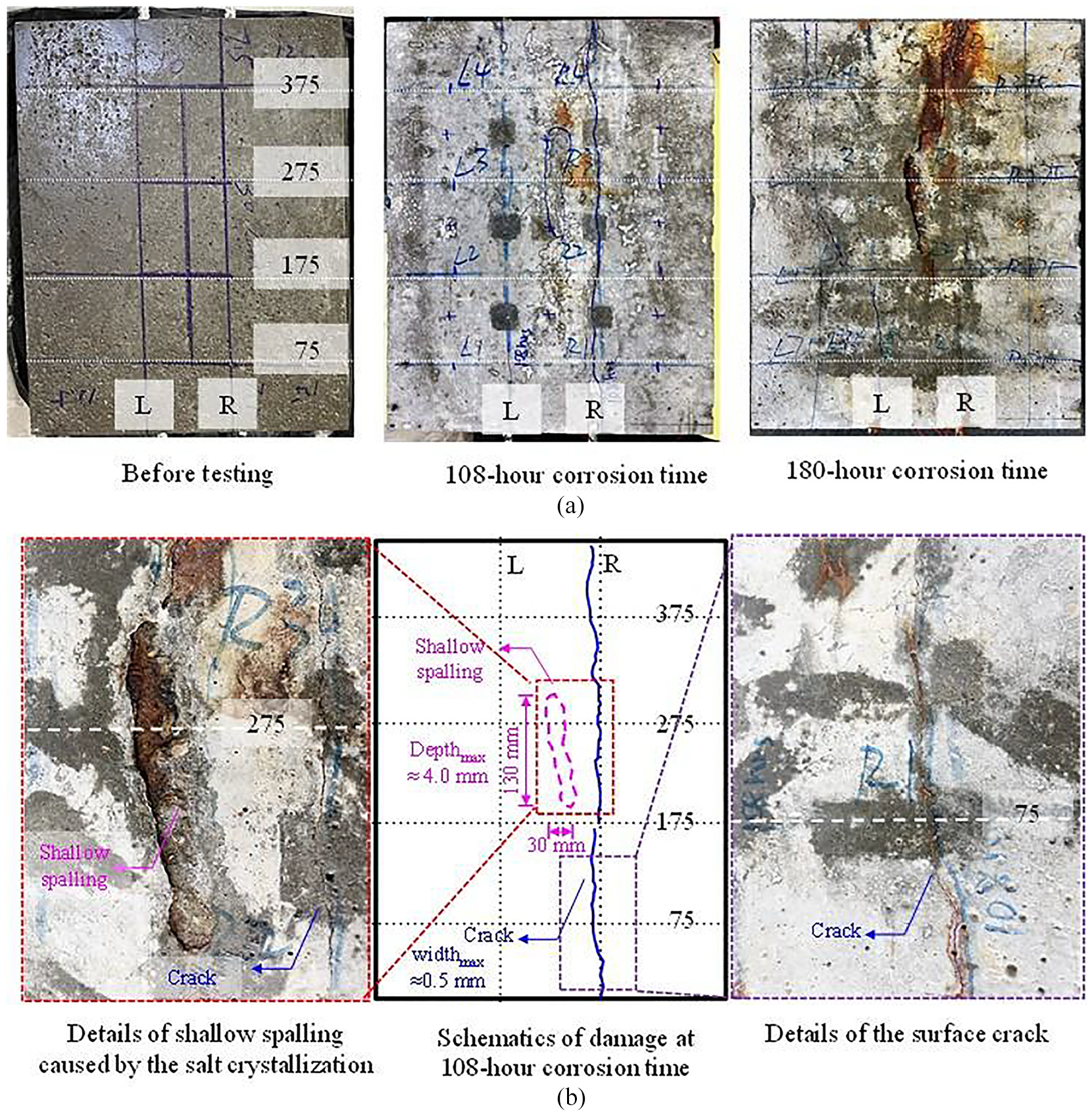
Visual inspection of the concrete slab over time: (a) visual inspection of the slab at different corrosion times and(b) details of shallow spalling and cracks at 108-h corrosion time.

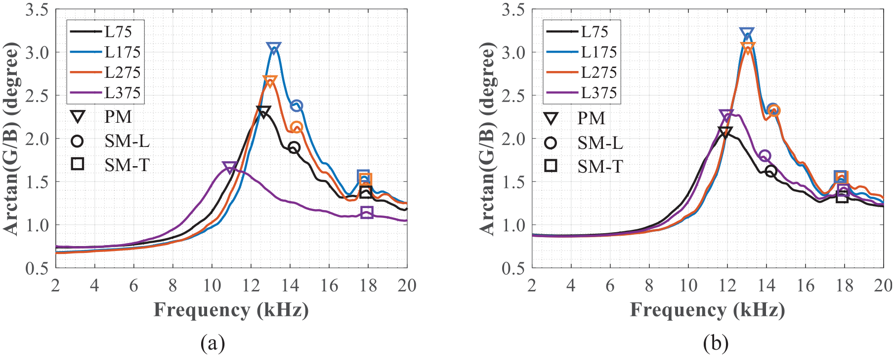
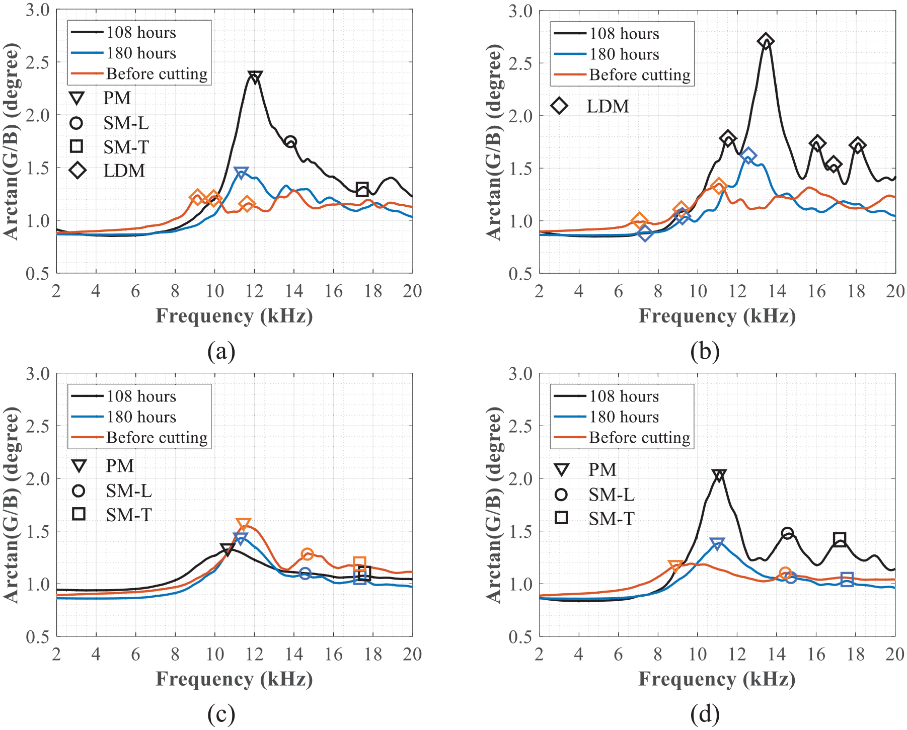
Figures 15 –18 present the signal spectra of different checkpoints at different corrosion statuses. The checkpoints are discussed in the sequence from two sides to the center area of the slab. Figure 15 shows the signal spectra of the checkpoints on Axes LO and RO. At Location LO175, no LDM peaks were observed in the signal spectra except for the reduction in the magnitude of the distinct peak (i.e., labeled by the lower triangle symbol) (Figure 15(a)). Peaks SM-LO referred to a slab mode excited on Axes LO or RO, slightly different from the mode SM-L because the global slab vibration modes were more or less related to the location of the PZT sensor on the concrete slab.⁵⁰ At Location LO275, multiple peaks appeared at the 108-h corrosion time, and the first resonance peak was 8.4 kHz (Figure 15(b)). The diamond markers in the figure denote the first three easily identified peaks as references. The signal pattern at 180 h was similar to that at 108 h, but the peaks moved leftward. For example, the first resonance peak moved leftward to 7.0 kHz. The pattern of the signal spectrum changed at the status “before cutting” (i.e., Step 5), compared with those at the 108-h and 180-h corrosion time. The signal spectrum weakened considerably, indicating that the new damage might have occurred because of slow corrosion in the 6-month placement and the transportation of the slab, as mentioned in Table 4. The first resonance peak moved to 5.4 kHz, and the two other peaks were captured at around 8.0 and 10.0 kHz. At Locations RO175 and RO275, as shown in Figures 15(c) and (d), respectively, the signal patterns remained unchanged, even with the reduced magnitude and slight changes in the sensor and slab mode.

Figure 15.

Signal spectra of the checkpoints on Axes LO and RO at different statuses: (a) LO175, (b) LO275, (c) RO175, and(d) RO275.

Figure 16.

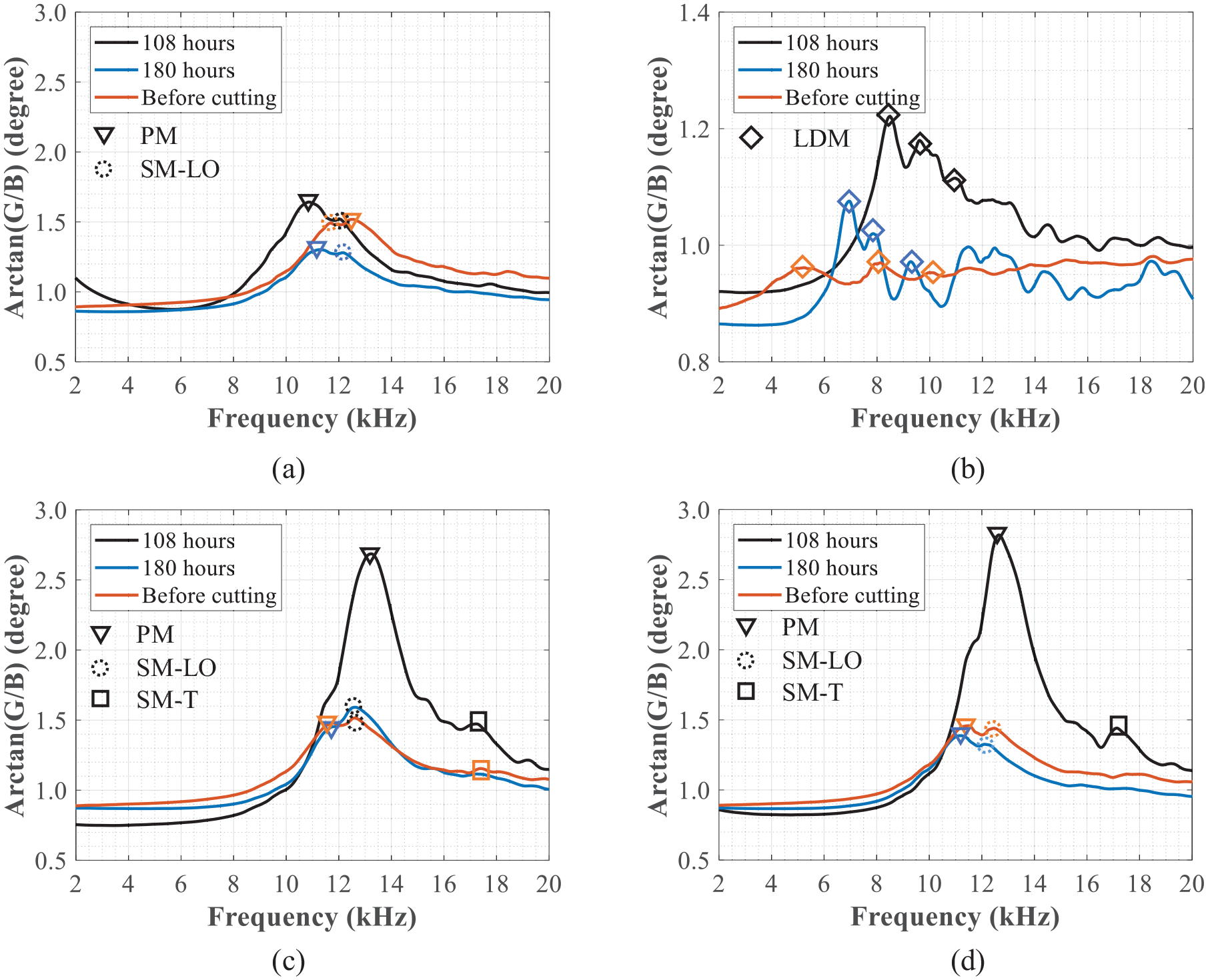
Signal spectra of the checkpoints above the rebars at different statuses: (a) L175, (b) L275, (c) R175, and (d) R275.

Figure 17.

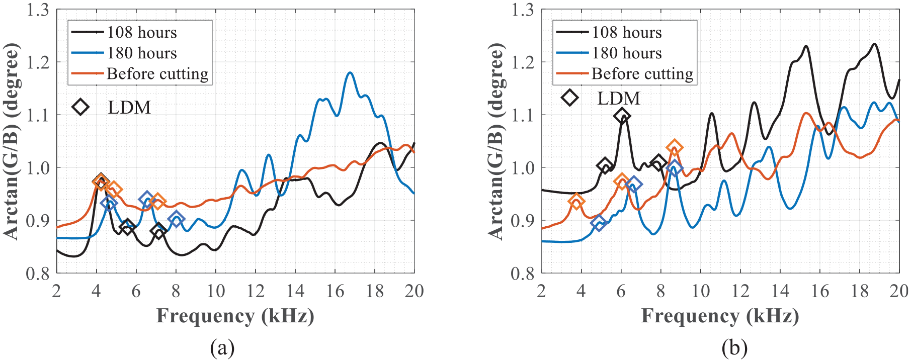
Signal spectra of the checkpoints above Axis-C at different statuses: (a) C175 and (b) C275.

Figure 18.

Maps of the first resonant frequencies.

Figure 16 presents the signal spectra of the checkpoints above the rebars (on Axes L and R) at different corrosion statuses. At Location L175, the signal patterns at 108- and 180-h corrosion time were consistent with those under the undamaged status (Figure 16(a)). The PZT sensor’s peak was larger than 11.0 kHz. At the status “before cutting,” dual peaks were observed below 10 kHz. The frequency of the first peak was 9.1 kHz, implying that the local damage was detected. At Location L275, multiple peaks labeled as diamond markers were found at 108 h (Figure 16(b)). The first peak appeared at 9.3 kHz and moved to 7.3 and 6.9 kHz at two other statuses. Although a continuous surface crack was observed above the right rebar (Figure 14(b)), it is interesting to observe that the pattern of the signal spectra in Figures 16(c) and (d) did not change considerably. Only at the “before cutting” status, the first dominant peak was moved to 9.6 kHz at Location L325.

Figure 17 presents the signal spectra close to Axis C. The sensor was installed 25 mm to the left of the original Axis C to avoid the uneven surface induced by shallow spalling. The signal spectra substantially changed at these two checkpoints, and multiple peaks starting from 3.5 kHz were observed. At Location C175, as shown in Figure 17(a), the first resonance peak moved rightward from 4.3 to 4.7 kHz as the corrosion time increased, which might be caused by the complicated changes in the boundaries. However, the first resonance peaks moved leftward to 4.2 kHz at the “before cutting” status. At Location C275, the signal spectra also presented multiple peaks moving leftward with increasing corrosion time (Figure 17(b)). The first resonance peak moved leftward from 4.0 to 3.5 kHz.

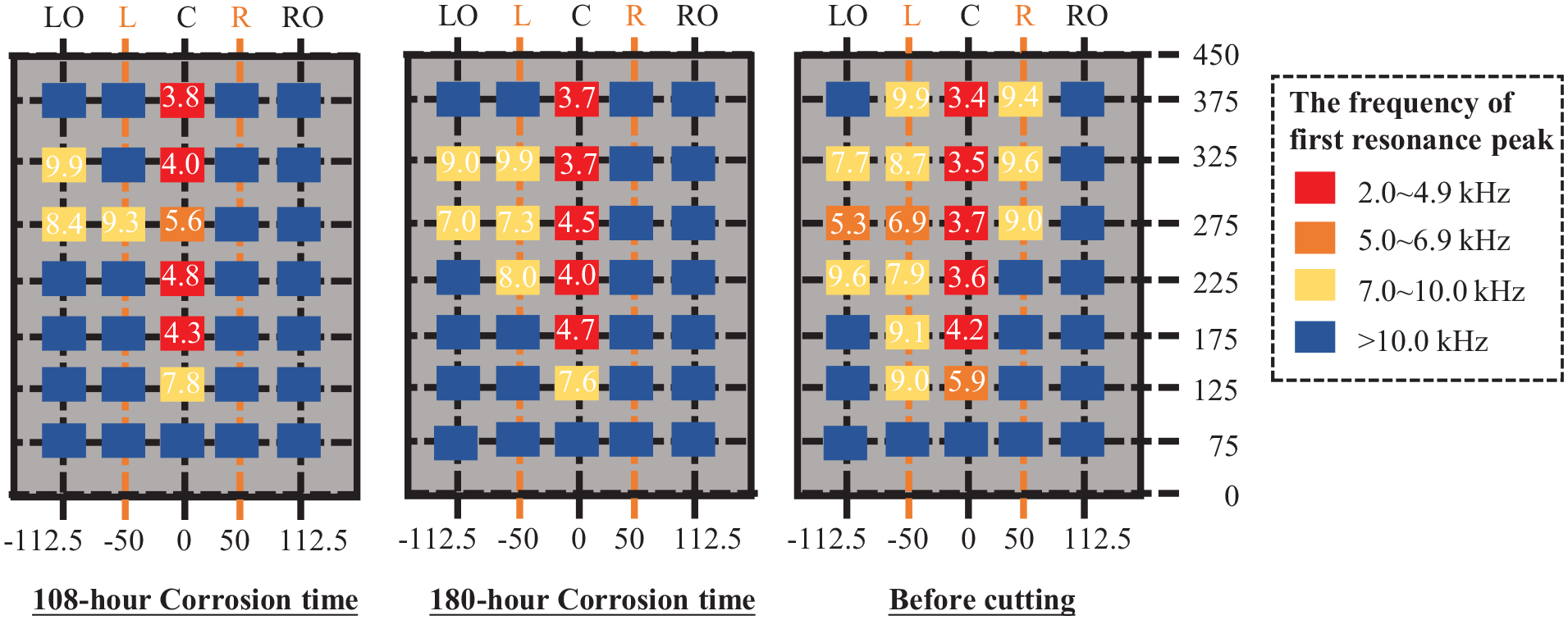
Figure 18 presents the maps showing the first resonant frequency in the selected frequency range, where four different colors are used to represent different frequency ranges and may correspond to different damage statuses. Red refers to the severe damage status, and blue refers to the healthy status. Yellow and orange denote intermediate statuses. The criterion behind this classification was as follows: (1) In a healthy status, the distinct peak corresponded to the sensor mode, which was influenced by the bonding conditions but was always larger than 10 kHz, as shown in Figure 13; and (2) In a damaged status, according to Equation (5), the first-order defect frequencies with defect sizes 100 × 100 × 15 mm³ and 125 × 125 × 10 mm³ are around 6.8 and 4.8 kHz, respectively, for the given material properties. Therefore, the frequency thresholds of 4.9, 6.9, and 10 kHz were used for classification, which was rather subjective and needs to be refined in the future. Although the surface crack was observed above the right-side steel rebar, the predicted delamination mainly appeared around the steel rebar on the left. As the corrosion time increased, more resonance peaks lower than the threshold were observed on the Axes LO and L, implying that the delamination may have occurred without visible surface phenomena. Based on the lowest frequency (i.e., 3.4 kHz) of the slab, the delamination area can be estimated using Equations (6), (8), and (9). The calculated lower and upper bounds of a were equal to 137 and 158 mm for square delamination with a 15-mm depth, respectively. For rectangular delamination, the estimated lower and upper bounds of a_w (short side) were 97 and 112 mm, respectively.

Slab cutting results

The concrete slab was cut to verify the evaluation results for the delamination. Figure 19 shows the concrete cutting equipment. The slab was fixed to avoid unwanted movement. The cutting machine’s blade had a 0.5 m diameter. The cutting machine moved along a sliding track during its operation. The cutting sections of the slab were along Axes 75, 175, 275, and 375.

Figure 19.

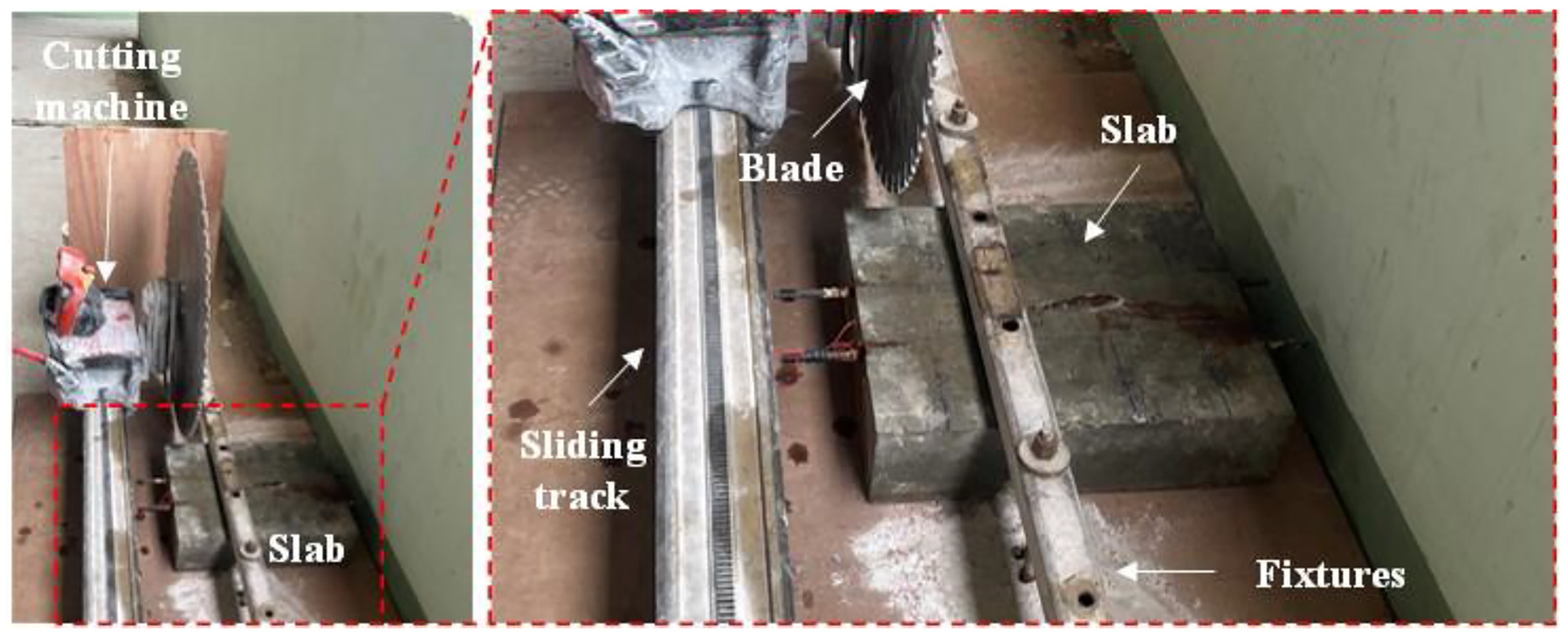
Setup for slab cutting.

Figure 20 shows the pictures of the cutting sections and the corresponding drawings of the crack distributions. As indicated in Figure 20(a), the damage level on the left rebar was much more severe than on the right, which may be attributed to the thinner concrete cover. This observation was consistent with the prediction shown in Figure 18, but it was very different from the surface visual inspection, indicating that the surface visual inspection could be unreliable. Regarding the comparison among different sections, Section 75 was healthy and had only two small cracks around the right rebar, indicating the effectiveness of the protection coating of the steel rebar in this section. By contrast, the protection at Section 375 failed, but the damage was successfully detected. Except for Section 75, the three other sections had two major inclined cracks on the left bar, which were relatively wide. These two cracks developed through the mortar and did not pass through the aggregates. The inclined cracks between the Axes LO and L had different depths at the end. The depths in Sections 375, 275, and 175 were 15, 3, and 2 mm, respectively. Meanwhile, the inclined cracks between Axes L and C propagated to the near-surface spalling. The observed damage levels of the four sections in Figure 20 agreed well with the prediction results of the proposed method in Figure 18.

Figure 20.

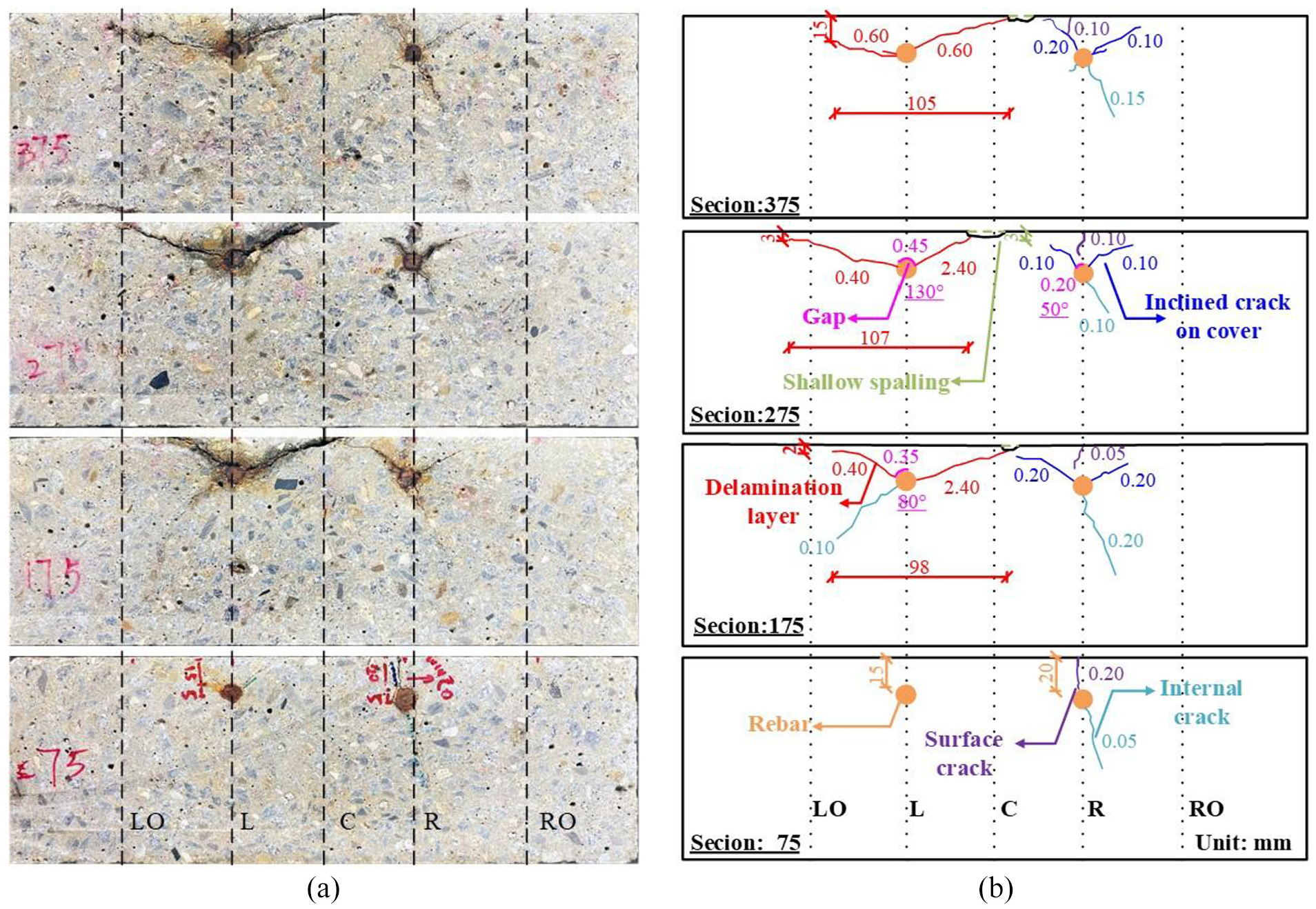
Pictures of the cutting sections and schematics of the crack distributions: (a) pictures of the four cutting sections and (b) schematics of the crack distributions (the value beside the crack in the same color is the maximum width, and the degree shown in pink refers to the angle extent relative to the center of the rebar).

Figure 20(b) draws the crack distributions to thoroughly understand the corrosion-induced damage. The value beside the crack in the same color is the maximum width of the crack measured by the feeler gauge. The cracks were divided into four categories, namely, delamination cracks in the cover (red), inclined cracks in the cover (blue), internal cracks (green), and surface cracks (purple). Notably, both the delamination and inclined cracks were essentially inclined cracks. They are divided by considering their maximum width and length. The maximum widths of the delamination cracks were at least 0.40 mm, and the lengths of the delamination cracks were around 100 mm. So, the delamination cracks could be considered nearly horizontal, causing a delamination layer with a separation plane roughly parallel to the surface. Whereas the maximum widths of the inclined cracks were not more than 0.2 mm, and their lengths were smaller than 70 mm. Among the four sections, only Section 275 had the delamination layer between the Axes LO and L, which is in good agreement with the detection results in Figure 18. The delamination cracks between Axes L and C propagated to the center axis in Sections 175, 275, and 375, which were well detected in Figure 18. The internal cracks in Figure 20(b) had relatively small widths and were not the focus of this study. Although the surface cracks could be observed visually, they did not initiate from the steel rebars, or in other words, they did not penetrate through the entire cover. The surface cracks perpendicular to the cover were caused by the expansion pressure from nonuniform rust, which induced tensile stress concentration on the point above the rebar.³¹ Aside from the cracks, different debonding gap (in pink) statuses at the interfaces between the concrete and rebars were shown at Locations L175, L275, and L275. The underlined numbers in Figure 20(b) presented the angle extent relative to the center of the rebar. The longest and largest gap occurred at Location L275, with a 130° relative angle and 0.45 mm width. The damage was also successfully detected using the proposed method.

The cutting results also provided geometric information on the delamination, allowing a quantitative comparison between the experimental results and the prediction results. The average width of the delamination layer, a_w, was equal to 103 mm, close to the estimated results (i.e., from 97 to 112 mm). Given that only four sections were cut, a_l could not be accurately measured.

To sum up, although the actual corrosion-induced delamination was more complicated than the simulated conditions, it was successfully detected, localized, and quantified by the proposed method in the presented laboratory experiments. Even invisible damage on the left side of the concrete slab was successfully detected, showing the effectiveness of the proposed detection method.

On-site testing validations

Given the successful numerical and experimental validations of the proposed method, on-site testing was conducted to further examine its applicability outside the laboratory environments and validate its real-world effectiveness.

Site and testing information

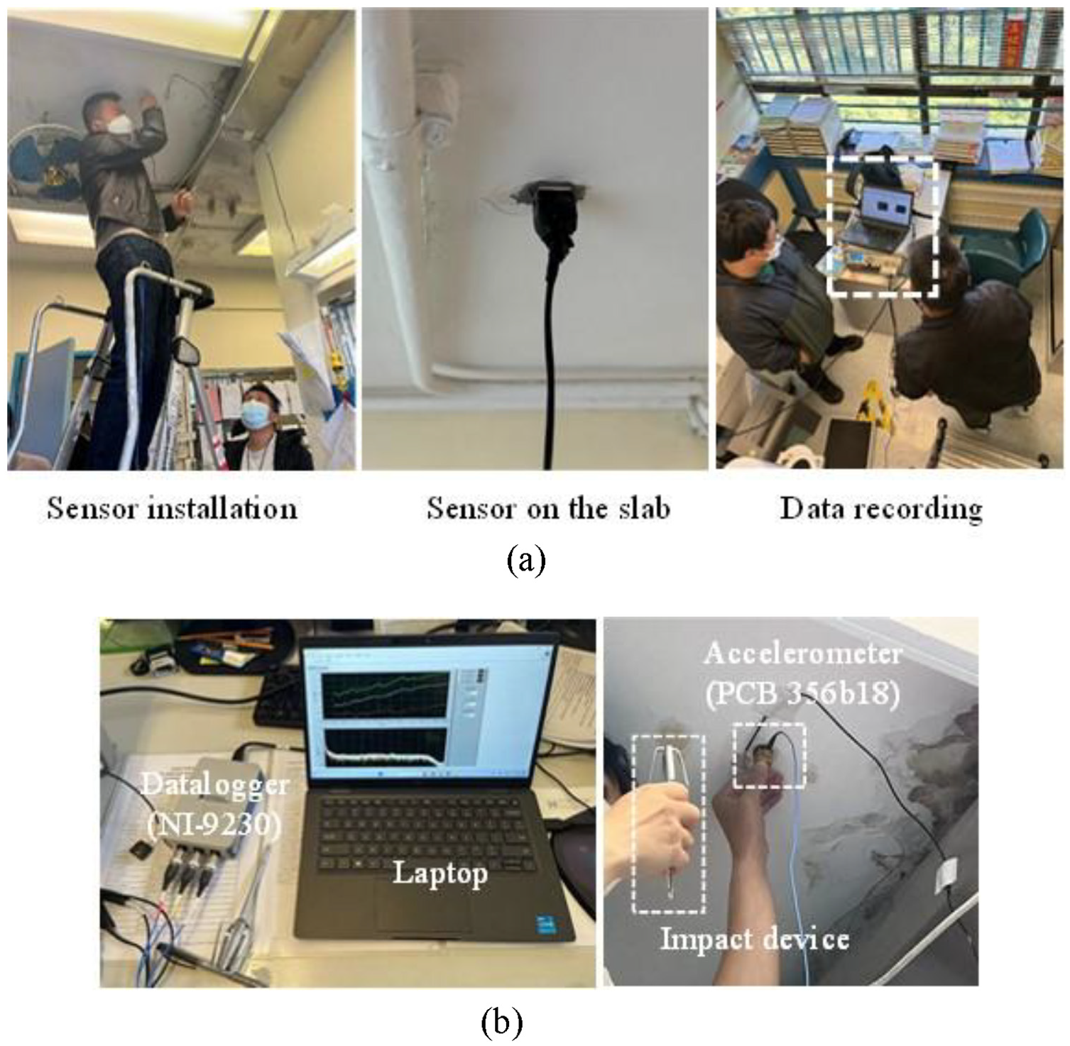
On-site testing using the movable PZT sensor and EMI technique was conducted in an old building in Hong Kong, whose structural details are unavailable. In addition to the proposed method, the traditional impact-echo method was also applied for comparison. Two tests were conducted during half a year. Figure 21 presents the measured areas and details of the testing techniques. The same sensor, bonding tape, device, and data acquisition system as those in the laboratory experiments were used for the EMI technique (Figure 21(a)). Figure 21(b) illustrates the equipment employed for the impact-echo method, including a compact data acquisition system (NI-9230) with a maximum sampling rate of 12.8 kS/s, a high-fidelity triaxial accelerometer (PCB 356b18), and a stainless steel bar.

Figure 21.

On-site testing procedures and details of the testing techniques: (a) EMI technique and (b) Impact-echo method.

Suspected delamination area and corresponding signals

After the careful examination of two rooms, a suspected delaminated area was confirmed. Figure 22(a) illustrates the suspected delaminated area and the arrangement of the checkpoints. After the first test, a fixed PZT patch with a size of 20 × 20 × 1.0 mm³ was also employed for comparison. The PZT patch was bonded to Point B by using quick-hardening epoxy (Devcon 14270). The surface of the concrete slab had a 3-mm thick plaster layer. No visible cracks were found on the surface. Figure 22(b) shows the EMI spectra recorded at these points, in which the signal spectra range from 2 to 20 kHz, considering the low sensitivity of the PZT sensor below 2 kHz, as discussed in the numerical part. The delamination could be easily identified in the tested area, except for Point D, from the spectral pattern. Compared with Point D, the magnitude of peaks in other points was relatively lower. Meanwhile, multiple peaks were captured below 10 kHz, especially at Point C. The frequencies of the first resonance peaks for Points A, B, C, D, and E are 4.9, 8.5, 3.6, 10.4, and 7.4 kHz, respectively. Under the assumption that the modulus of elasticity of concrete was equal to 30 GPa, the density and Poisson’s ratio of concrete equaled 2368 kg/m³ and 0.2, respectively. The concrete cover was assumed to be 20 mm. The upper bound of a for Points A, B, C, and E were 130, 101, 161, and 101 mm, respectively. By assuming a square delaminated area, the average dimension a for the four points was 123 mm, with a standard deviation of 29 mm. When the lowest frequency at Point C (i.e., 3.6 kHz) was used, the lower and upper bounds of delaminated dimension a were 136 and 161 mm, respectively.

Figure 22.

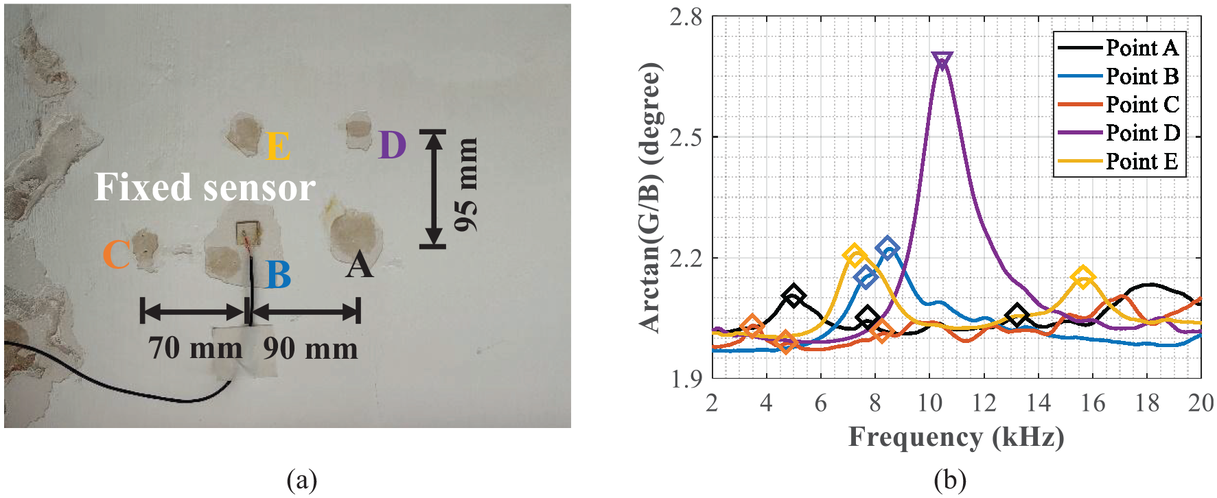
Suspected delamination area, checkpoints, and the corresponding EMI signals: (a) suspected delamination area and checkpoints and (b) signal spectra at different points.

Figure 23 plots the signal from the impact-echo methods at Points A and C. Given the maximum sampling rate of 12.8 kS/s, the maximum frequency reached 6.4 kHz after applying the frequency response function. However, the resonance peaks were difficult to identify even in the log-scale plot. The peaks at 5.2 and 3.6 kHz were captured by the impact-echo method at Points A and C, respectively, which were consistent with those captured by the EMI technique. This consistency confirms the effectiveness of the proposed method. Meanwhile, the resonance peaks in the signal spectrum of the EMI technique were much easier to identify, indicating the technique’s high signal-to-noise ratio and application advantages.

Figure 23.

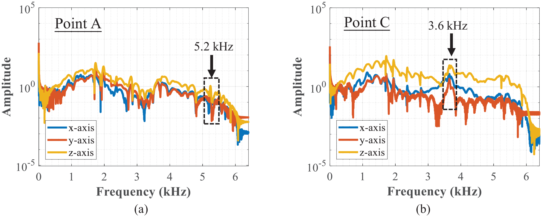
Signal spectra from the impact-echo method: (a) Point A and (b) Point C.

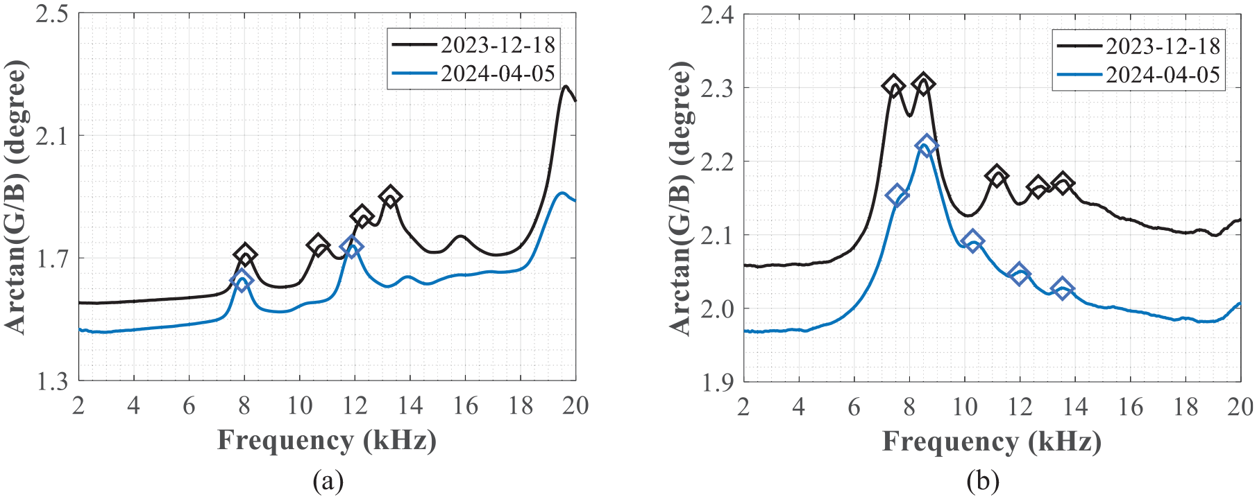
Figure 24 presents the recorded signal spectra at Point B from two types of PZT sensors in two different tests. The signal spectra obtained at two different dates were generally consistent. Meanwhile, the first local defect resonance peak moved slightly (Figure 24(a)). In general, the movable sensor could produce stable and consistent results, as indicated in Figure 24(b). According to the results, movable PZT sensors can be a convenient alternative to traditional fixed PZT sensors, particularly for short-term inspection of suspected areas.

Figure 24.

Signal spectra recorded at Point B at different times and with different sensors: (a) fixed sensor and (b) movable sensor.

Cover opening for verification

After the assessment in the previous section, the tested area was opened by using a driller. The driller easily removed a layer with around 10 mm thickness. The opened area had about 250 mm length and 230 mm width, containing an apparent flat interface caused by delamination, as shown in Figure 25(a). If the actual delamination depth (i.e., 10 mm) was substituted into Equations (6) and (8), the upper bounds of a for the checkpoints A, B, C, and E were 103, 97, 126, and 90 mm, respectively. The average value of a based on the four checkpoints was 104 mm. The predicted a value was within the opening area, indicating fair consistency. An 80-mm long and 70-mm wide brown area was found on this flat surface. After removing the concrete in the brown area, a corroded rebar with a 7 mm diameter was found (Figure 25(b)). Delamination evidence was also found at the boundary of the opening area, as shown in Figure 25(c). Figure 25(d) presents the collected fragments after the opening. The thickness of the concrete fragments was around 7 mm after deducting the thickness of the plaster. The abovementioned information indicates that the expansion of the steel rebar caused delamination along a weak interface in the tested area. In summary, the on-site testing results validated the proposed EMI technique’s effectiveness in detecting the concrete cover’s delamination.

Figure 25.

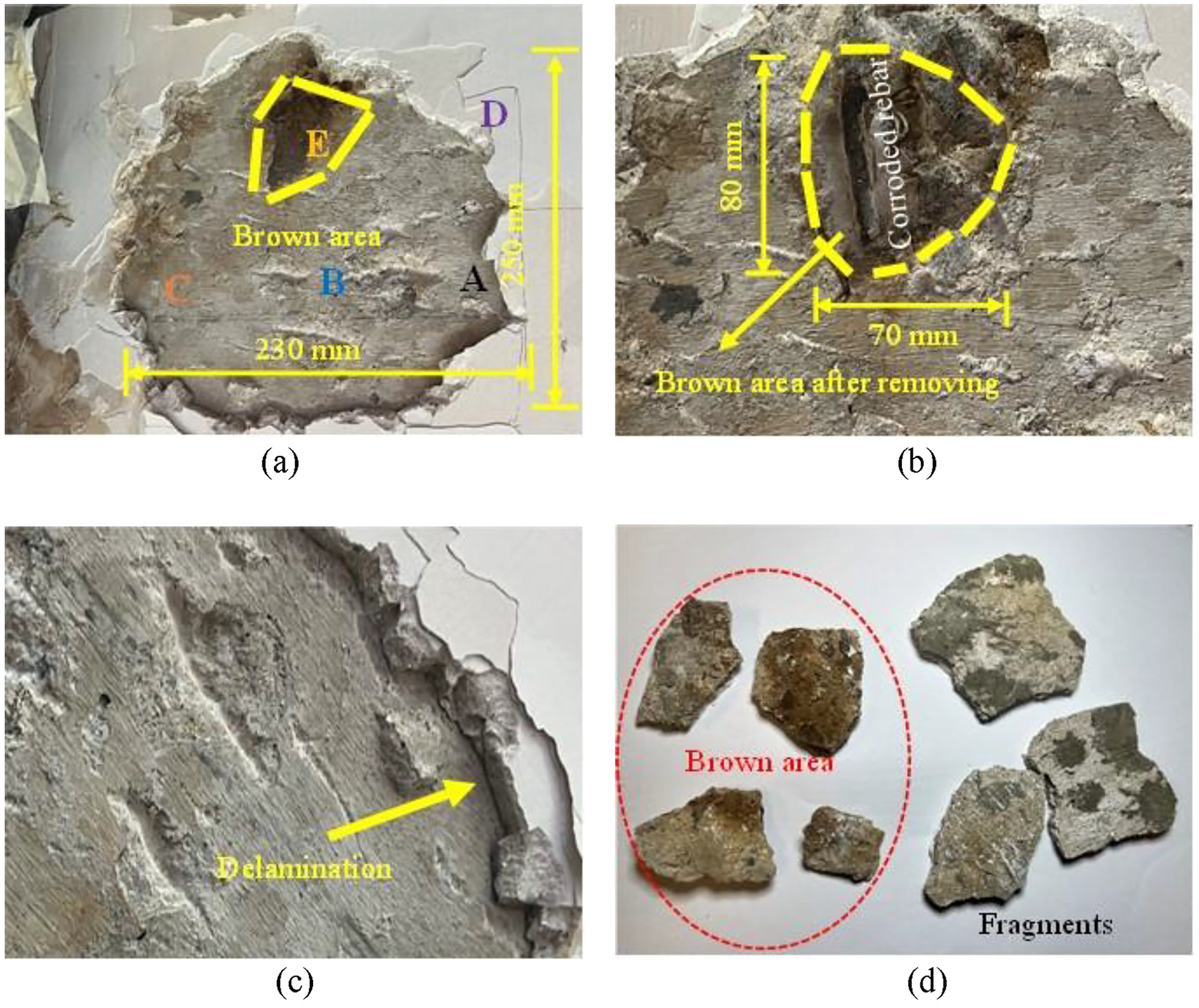
Opening results for verification: (a) opening up results, (b) corroded rebar, (c) delamination, and (d) fragments.

Conclusions

An improved baseline-free EMI technique using a movable sensor for detecting the delamination of the concrete cover was proposed, validated numerically and experimentally, and applied on-site. The following major conclusions were obtained:

The spectral patterns and characteristics could be used to quickly determine the concrete cover’s delamination, confirming the proposed method’s effectiveness in detecting and localizing delamination damage. In a healthy condition, only a distinct resonance peak above 10 kHz (corresponding to the sensor mode) could be observed; when the tested area was delaminated, multiple peaks below 10 kHz (corresponding to local defect resonances) could be captured.

The local defect resonances of the delaminated area were highly related to the defect size and material properties. The correlations between the first-order frequency of the local defect resonance and defect size were established numerically for a quick, approximate assessment.

The local defect resonance peaks were insensitive to the sensor’s bonding materials and the slab’s boundary conditions.

The proposed method presented the signal spectra with a high signal-to-noise ratio. Hence, it can be directly implemented for on-site testing.

While the primary focus of this study is on detecting the delamination of the concrete cover in RC slabs, the proposed NDT method can be easily extended to long-term monitoring at crucial locations and the detection of the delamination of other materials and structures, paving a promising avenue for future research and application. The improvement of this study lies in choosing more appropriate sensors and bonding materials to ensure the use of higher frequency signals to detect smaller and deeper delamination.

Footnotes

Declaration of conflicting interests

The author(s) declared no potential conflicts of interest with respect to the research, authorship, and/or publication of this article.

Funding

The author(s) disclosed receipt of the following financial support for the research, authorship, and/or publication of this article: The Theme-based Research Scheme (Numbers T22-502/18-R and T22-501/23-R) and Research Impact Fund (Number R5006-23), the Hong Kong Branch of the National Rail Transit Electrification and Automation Engineering Technology Research Center (Number K-BBY1), and the Hong Kong Polytechnic University (Numbers CDB6, CDKN, W02L).

ORCID iDs

Xiong Sha

Songye Zhu

References

Zhang

Liu

, et al. Corrosion-induced spalling of concrete cover and its effect on shear strength of RC beams. Eng Fail Anal 2021; 127: 105538.

Zhu

. Effects of freeze-thaw damage on the bond behavior of concrete and enhancing measures. Construct Build Mater 2019; 196: 375–385.

Zheng

Wang

Zhang

, et al. Research progress of the thermophysical and mechanical properties of concrete subjected to free-thaw cycles. Construct Build Mater 2022; 330: 127254.

Press Releases, The Government of the Hong Kong Special Administrative Region. https://www.info.gov.hk/gia/general/200101/17/0117185.htm (2001, accessed 18 December 2024)

Shokouhi

Wöstmann

Schneider

, Nondestructive detection of delamination in concrete slabs: multiple-method investigation. Transp Res Rec 2011; 2251(1): 103–113.

Sajid

Chouinard

Taras

. Developing a new understanding of the impulse response tests for defect detection in concrete plates. J Eng Mech 2022; 148 (1): 04021125.

Popovics

Sim

. Analysis of vibration for regions above rectangular delamination defects in solids. J Sound Vib 2013; 332: 1766–1776.

Gucunski

. Nondestructive testing to identify concrete bridge deck deterioration. Transportation Research Board, National Research Council; 2013.

Kee

Gucunski

. Interpretation of flexural vibration modes from impact-echo testing. J Infrastruct Syst 2016; 22(3): 04016009.

10.

Liang

Sun

Rogers

. (1994). Coupled electro-mechanical analysis of adaptive materials systems-determination of the actuator power consumption and system energy transfer. J Intell Mater Syst Struc 1994; 5(1): 12–20.

11.

Migot

Giurgiutiu

. Numerical and experimental investigation of delamination severity estimation using local vibration techniques. J Intell Mater Syst Struc 2023; 34(9): 1057–1072.

12.

Zagrai

Giurgiutiu

. Electro-mechanical impedance method for crack detection in thin plates. J Intell Mater Syst Struc 2002; 12(10): 709–718.

13.

Sha

Zhu

. A baseline-free electromechanical impedance resonance method for measuring the modulus of elasticity of concrete cubes using surface-bonded PZT patches. Struct Control Health Monit 2024; 2024: Article ID 6153935, 18 pages.

14.

Kong

. Improved method to determine Young’s modulus for concrete cylinders using electromechanical spectrum: principle and validation. J Aerosp Eng 2020; 33(6): 04020079.

15.

Soh

Tseng

Bhalla

, et al. Performance of smart piezoceramic patches in health monitoring of a RC bridge. Smart Mater Struct 2000; 9: 533–542.

16.

Bois

Hochard

. Monitoring of laminated composites delamination based on electro-mechanical impedance measurement. J Intell Mater Syst Struc 2004; 15(1): 59–67.

17.

Roth

Giurgiutiu

. Structural health monitoring of an adhesive disbond through electromechanical impedance spectroscopy. Int J Adhes Adhes 2017; 73: 109–117.

18.

Gresil

Giurgiutiu

, et al. Predictive modeling of electromechanical impedance spectroscopy for composite materials. Struct Health Monit 2012; 11(6): 671–683.

19.

Zahedi

Huang

. Time-frequency analysis of electromechanical impedance (EMI) signature for physics-based damage detections using piezoelectric wafer active sensor (PWAS). Smart Mater Struct 2017; 26: 055010.

20.

Liu

Paurobally

. Robust damage metric in terms of magnitude and phase for impedance-based structural health monitoring, Struct Health Monit 2009; 8(4): 303–311.

21.

Lim

Smith

Padilla

, et al. Monitoring of concrete curing using the electromechanical impedance technique: review and path forward. Struct Health Monit 2021; 20(2): 604–636.

22.

Yang

Lim

Soh

. Practical issues related to the application of the electromechanical impedance technique in the structural health monitoring of civil structures: II. Numerical verification. Smart Mater Struct 2008; 17: 035009.

23.

Lin

Luo

, et al. Temperature effect on electromechanical admittance-based concrete structural health monitoring, Struct Health Monit 2009; 19(3): 661–692.

24.

Tenreiro

AFG

Lopes

da Silva

. A review of structural health monitoring of bonded structures using electromechanical impedance spectroscopy. Struct Health Monit 2022; 21(2): 228–249.

25.

Giurgiutiu

. Structural health monitoring: with piezoelectric wafer active sensors. 2nd ed. San Diego, CA, USA: Elsevier Academic Press; 2014.

26.

ASTM E650/E650M: 2017e. Standard guide for mounting piezoelectric acoustic emission sensors. West Conshohocken PA: American Society for Testing and Materials; 2017.

27.

Theobald

Zeqiri

Avison

. Couplants and their influence on AE sensor sensitivity. In: 28th European Conference on Acoustic Emission Testing, Krakow, Poland, 17–19 September 2008.

28.

Ozman

Safaei

Lan

, et al. A novel accelerometer mounting method for sensing performance improvement in acoustic measurements from the knee. J Vib Acoust 2021; 143(3): 031006.

29.

Solodov

Rahammer

Kreutzbruck

. Analytical evaluation of resonance frequencies for planar defects: Effect of a defect shape. NDT & E Int 2019; 102: 274–280.

30.

Zhang

Ling

Guan

. Finite element modeling of concrete cover crack propagation due to non-uniform corrosion of reinforcement. Construct Build Mater 2017; 132: 487–499.

31.

RKL

Zhang

. A novel elastic-body-rotation model for concrete cover spalling caused by non-uniform corrosion of reinforcement. Construct Build Mater 2019; 213: 549–560.

32.

Chen

Pan

. Mesoscopic simulation of steel rebar corrosion process in concrete and its damage to concrete cover. Struct Infrastruct Eng 2016; 13(4): 478–493.

33.

Song

Lim

Sohn

. (2013). Electromechanical impedance measurement from large structures using a dual piezoelectric transducer. J. Sound Vib. 2013; 332: 6580–6595.

34.

Narayanan

Kocherla

Subramaniam

KVL

. Understanding the coupled electromechanical response of a PZT patch attached to concrete: influence of substrate size. Measurement 2018; 124: 505–514.

35.

Tenek

Henneke

Gunzburger

. Vibration of delaminated composite plate and some application to non-destructive testing. Compos Struct 1993; 23: 253–262.

36.

Solodov

Bai

Busse

. Resonant ultrasound spectroscopy of defects: Case study of flat-bottomed holes. J Appl Phys 2013; 113: 223512.

37.

Zhang

, et al. Quantitative assessment of delamination in composites using multiple local-defect-resonance modes. J Sound Vib 2024; 589: 118499.

38.

Zheng

Lawanwisut

, et al. Concrete delamination caused by steel reinforcement corrosion. J Mater Civil Eng 2007; 19(7): 591–600.

39.

Zhang

RKL

. Experimental investigation of process of corrosion-induced cover delamination using digital image correlation. Construct Build Mater 2021; 312: 125287.

40.

Jenq

Chang

. Characterization of piezo-film sensors for direct vibration and impact measurements. Exp Mech 1995; 35: 224–232.

41.

Ono

. Through-transmission characteristics of AE sensor couplants. J Acoust Emiss 2017; 34: 1–11.

42.

De Angelis

Meo

Almond

, et al. A new technique to detect defect size and depth in composite structures using digital shearography and unconstrained optimization. NDT&E Int 2012; 45: 91–96.

43.

Sansalone

Streett

. Impact-echo: Nondestructive evaluation of concrete and masonry. Jersey Shore, PA, USA: Bullbrier Press; 1997.

44.

Goodacre

. Explanatory analysis of spectroscopic data using machine learning of simple, interpretable rules. Vib Spectrosc 2003; 32: 33–45.

45.

Xue

Sun

Yang

, et al. Advances in the application of artificial intelligence-based spectral data interpretation: a perspective. Anal Chem 2023; 95: 13733–13745.

46.

Mangat

Elgarf

. Flexure strength of concrete beams with corroding reinforcement. ACI Struct J 1999; 96(1): 149–158.

47.

El Maaddawy

Soudki

. (2003). Effectiveness of impressed current technique to simulate corrosion of steel reinforcement in concrete. J Mater Civil Eng 2003; 15(1): 41–47.

48.

Ting

MZY

Wong

Rahman

, et al. Deterioration of marine concrete exposed to wetting-drying action. J Cleaner Prod 2021; 278: 123383.

49.

Cai

, et al. Skin effect of chloride ingress in marine concrete: a review on the convection zone. Construct Build Mater 2020; 262: 120566.

50.

Zhou

Liang

Rogers

. Integration and design of piezoelectric patch actuators. J Intell Mater Syst Struc 1995; 6(1): 125–133.