Corrosion quantitative monitoring based on dual-modal electromechanical impedance and bidirectional multilevel fusion network

Abstract

Electromechanical impedance (EMI) technology has been widely used in structural health monitoring, yet its potential has been limited by conventional impedance measurement methods. This study proposes a novel axial and bending modal excitation method for EMI measurement, enabling simultaneous capture of dual-modal vibration responses. Based on these dual-modal characteristics, a novel bidirectional multilevel fusion network framework for EMI signal processing was proposed. The innovations of this study include (1) a logarithmic frequency dual attention module was designed, where first-order derivative attention mechanism captures instantaneous signal changes, second-order derivative attention mechanism captures curvature features, and fusion attention combines the advantages of both, improving the training accuracy of difficult-to-fit signals to 92.5%. (2) A bidirectional-attention multistage fusion network was proposed. This network adopts an innovative additive fusion strategy to effectively avoid gradient vanishing, fully utilizes the complementary features of axial and bending vibration modes, achieves deep information fusion and synergistic enhancement, enables the model to comprehensively grasp corrosion characteristics from different dimensions, and improves the training accuracy from 82.04% and 92.5% in single-modal scenarios to 100%. The method also demonstrated excellent noise resistance under various signal-to-noise ratio conditions, maintaining reliable performance in complex monitoring environments. These results confirm that the proposed dual-modal measurement method, combined with the fusion framework, provides an enhanced solution for EMI-based damage detection, offering improved sensitivity and reliability. This work establishes a new paradigm for EMI signal acquisition and processing in structural health monitoring applications.

Keywords

Electromechanical impedance dual-modal vibration multilevel fusion network damage detection structural health monitoring

Introduction

Structural health monitoring has become increasingly critical in fields such as energy infrastructure, chemical engineering, and marine engineering, with significant implications for equipment safety and reliability. Previous research indicates that structural damage is one of the main causes of industrial equipment accidents, resulting in severe economic losses annually.¹ Particularly in complex service environments, such as marine and atmospheric conditions, the challenges of damage detection and monitoring become more pronounced. Mahmoodian’s research demonstrates that preventive maintenance strategies incorporating advanced monitoring technologies can reduce life-cycle costs by approximately 25%–35% compared to reactive maintenance, while significantly improving system reliability.² Various nondestructive testing technologies have been developed to address these challenges. Vasagar et al.³ systematically reviewed existing detection methods, comparing electromagnetic and acoustic approaches. While single-modal detection methods such as magnetic flux leakage (MFL),⁴ ultrasonic testing,⁵ and eddy current testing⁶ have shown effectiveness in specific scenarios, they often face limitations in providing comprehensive structural health information. Advanced sensing technologies like fiber Bragg grating (FBG)-based systems⁷ and specialized monitoring probes⁸ have demonstrated advantages in continuous monitoring, yet the challenge of integrating and processing multimodal sensor data remains significant. Moreover, the widespread implementation of these technologies is often constrained by their high costs, with ultrasonic arrays and distributed fiber-optic systems requiring substantial initial investment and specialized maintenance expertise. This economic consideration has driven the search for more cost-effective monitoring solutions.

EMI as an emerging structural health monitoring method, demonstrates unique advantages in corrosion damage detection. Annamdas et al.⁹ explained the basic principles of EMI technology, confirming that the coupling effect between lead zirconate titanate and structures is the key mechanism for corrosion monitoring. Talakokula et al.^10,11 pioneered the application of EMI technology in concrete rebar corrosion monitoring, with their research showing significant correlation between admittance characteristics and corrosion levels. EMI technology has been applied in steel structures and wooden structures.^12,13 Na and Park¹⁴ experimentally verified the feasibility of EMI technology in detecting metal pipeline wall thickness loss, providing new insights for pipeline corrosion monitoring. Wang et al.¹⁵ proposed and validated a quantitative rod-type corrosion measurement probe based on piezoelectric stack and EMI technology, proving its reliability and accuracy in corrosion monitoring through theoretical modeling and experimental verification. Subsequently, Wang et al.¹⁶ developed a conical corrosion measurement probe based on EMI technology, successfully achieving quantitative monitoring of pipeline corrosion through combined finite element analysis and experimental validation. The reusable piezoelectric sensors developed by Raju et al.¹⁷ showed good performance in corrosion assessment, particularly with their nonbonded configuration showing higher sensitivity to corrosion damage. Liu et al.¹⁸ studied the application of EMI technology in concrete damage diagnosis, demonstrating its effectiveness in structural damage detection and characterization through impedance feature analysis. Zhang et al.¹⁹ achieved breakthroughs in environmental factor compensation, significantly improving corrosion monitoring accuracy. In summary, EMI technology offers advantages of high sensitivity, rapid response, and strong autonomous monitoring capabilities. However, existing research still faces challenges. First, the quantitative relationship between impedance characteristics and corrosion degree needs further investigation. Second, signal processing and feature extraction methods in complex working conditions need further improvement. Addressing these challenges, the development of EMI corrosion monitoring methods with enhanced environmental adaptability and high precision holds substantial theoretical value and significant engineering application potential.

Deep learning technology has made significant progress in EMI signal processing and structural health monitoring. De Oliveira et al.²⁰ pioneered a novel structural health monitoring method combining PZT sensors with convolutional neural networks, integrating traditional sensing technology with advanced deep learning methods to achieve more accurate damage detection and classification. Chen et al.²¹ proposed a quantitative monitoring method for bolt loosening that combines multichannel piezoelectric active sensing and attention mechanism based convolutional neural networks, improving the accuracy of bolt loosening recognition through attention-enhanced deep learning models. Li et al.²² proposed a method combining EMI technology with convolutional neural networks to address the quantitative assessment of concrete structure damage under different temperature conditions, improving temperature adaptability and accuracy of damage identification. Yan et al.²³ developed an intelligent monitoring system integrating EMI with neural networks for real-time monitoring and evaluation of early hydration and setting processes in cement mortar, achieving intelligent characterization of early cement material properties. Ai et al.²⁴ developed an automated method based on convolutional neural networks to identify compressive stress and damage states of concrete specimens by learning electromechanical admittance features, achieving intelligent assessment of concrete structure conditions. Ai et al.²⁵ proposed a one-dimensional convolutional neural network-based EMI deep learning method for concrete structure damage identification, achieving efficient damage feature extraction and recognition through direct processing of raw impedance signals. Yang et al.²⁶ proposed a novel nondestructive testing method based on EMI for evaluating fiber content in concrete, providing a new solution for rapid, nondestructive assessment of concrete fiber content. Ai et al.²⁷ proposed a two-dimensional convolutional neural network-based EMI deep learning method, achieving precise quantitative assessment of concrete structure damage by converting impedance signals into two-dimensional feature maps. These research findings demonstrate the enormous potential of deep learning technology in structural health monitoring. The application of this technology to quantitative monitoring of pipeline corrosion has important practical implications. However, most existing methods rely on single-modal analysis and traditional frequency shift techniques, which limit their ability to capture comprehensive structural information and process complex damage features effectively. The integration of multimodal information remains largely unexplored, presenting a significant opportunity for improving monitoring accuracy and reliability.

To address these limitations and advance the field of pipeline corrosion monitoring, there is a pressing need for methods that can effectively process and integrate multimodal EMI signals while leveraging the advantages of deep learning technology. This study proposes a dual-modal EMI monitoring method integrated with a bidirectional multilevel fusion network. Traditional single-modal EMI methods face challenges in achieving comprehensive structural health monitoring, while conventional frequency shift analysis shows limitations in extracting complex damage features. The hardware core of this method involves attaching piezoelectric patches to the surface of metal probes, using EMI harmonic excitation to generate axial vibration mode and bending vibration mode respectively. These dual-modal signals provide complementary information about the structural state, as different vibration modes exhibit varying sensitivities to structural changes. When structural changes occur, they cause shifts in characteristic resonance frequencies of both modes, which can be captured through impedance spectroscopy. Unlike traditional frequency shift linear analysis, this study innovatively employs a bidirectional multilevel fusion network to process the dual-modal impedance spectral data. The fusion process extracts and integrates channel attention and temporal attention from both vibration modes, completing the comprehensive feature extraction through residual connections. This approach enables more robust and sensitive structural health monitoring by leveraging the complementary advantages of different vibration modes.

The remainder of this study is organized as follows: Section “Proposed framework” presents the proposed framework. Section “Logarithmic frequency dual attention module” introduces the logarithmic frequency dual attention signal processing method and novel multimodal fusion network structure. Section “Bidirectional-attention multistage fusion network” describes the design of corrosion probes capable of receiving both vibration modal signals for accelerated corrosion testing. Section “Experimental verification” analyzes and discusses the theoretical and experimental results. Section “Result analysis” concludes the article.

Proposed framework

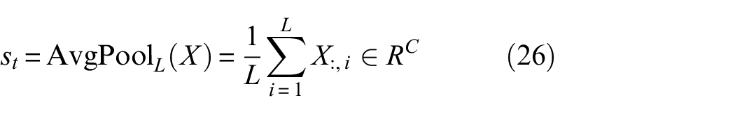
Drawing inspiration from Alexander et al.,²⁸ this study proposes novel axial and bending modal excitation methods. To address the issue that single-modal EMI signals cannot fully reflect structural characteristics, a dual-modal EMI fusion method that comprehensively captures structural feature information by combining axial and bending signal modalities was proposed in this study. To address the problem of signals spanning multiple orders of magnitude causing lower-order signals to be ignored, a logarithmic frequency dual attention signal processing method was proposed to learn features from signals of different magnitudes. Based on this, a bidirectional multilevel fusion network was designed, which consists of intermediate fusion and final fusion stages to achieve deep feature extraction and fusion of multimodal signals. The designed bidirectional attention fusion module effectively combines two inputs through channel attention and temporal attention, and further deepens feature learning through residual connections. This method successfully fuses signals from different vibration modalities, enhancing the richness and discriminative ability of feature representation, providing technical support for structural health monitoring and fault diagnosis. The proposed method flow was shown in Figure 1. BMFN is a dual-parallel network structure where the bending modal signal first undergoes feature enhancement preprocessing through Logarithmic frequency dual attention module (LFDM), while the axial modal signal directly inputs to the convolutional layer, and finally achieves bidirectional feature fusion of both modal signals through intermediate fusion modules and final fusion modules (BFM modules). This design fully utilizes LFDM’s advantages in processing bending modal signals and achieves effective integration of different modal information through BFM modules.

Figure 1.

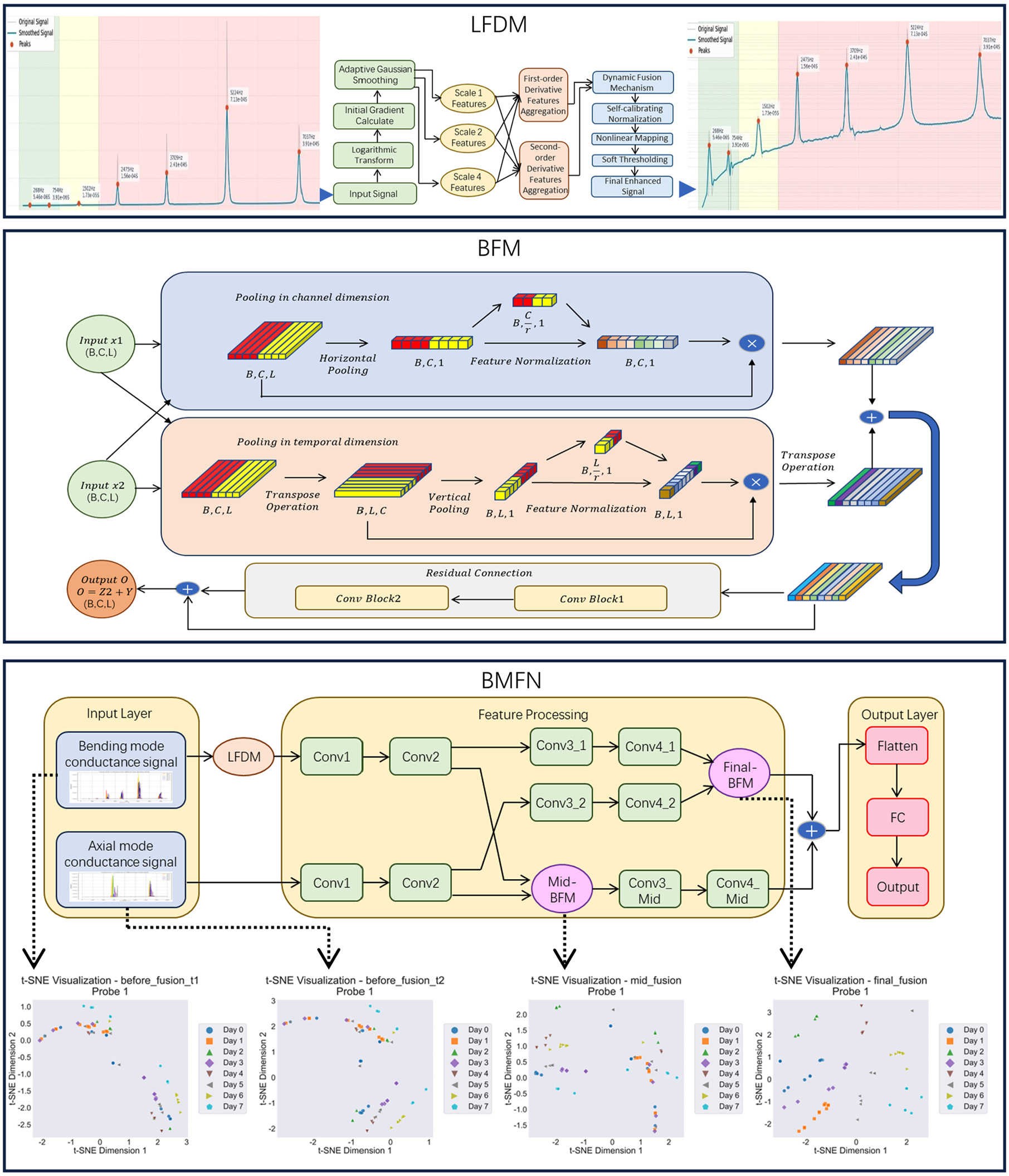
Method flowchart.

Logarithmic frequency dual attention module

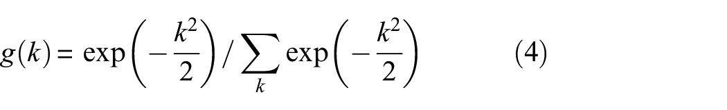
This section proposes a logarithmic domain multiorder derivative adaptive signal processing method, which is built upon three core theoretical foundations. First, logarithmic domain signal processing theory provides an effective method for handling large dynamic range signals. Through logarithmic transformation, it compresses signal dynamic range, enhances weak signal features, and makes signal feature distribution more uniform, thereby laying the foundation for subsequent processing. Adaptive smoothing theory is the second theoretical pillar of this algorithm, which overcomes the drawback of traditional fixed-window smoothing methods that easily cause loss of signal details. By dynamically adjusting the smoothing degree according to local gradients, it maintains more details in areas of dramatic signal changes while performing stronger smoothing in gentle areas, achieving optimal balance between signal enhancement and denoising. Finally, multiorder Gaussian derivative theory provides mathematical tools for feature extraction. First-order derivatives capture signal change trends and edge features, while second-order derivatives reflect curvature changes and detect local extrema and inflection points. The combination of these multiorder derivatives enables a more complete characterization of local structural information. The organic integration of these three theoretical foundations combines traditional signal processing theory with modern deep learning methods. This integration maintains algorithmic interpretability while enhancing the ability to process complex signals, thus providing solid theoretical support for subsequent algorithm design.

The design philosophy of LFDM is developed to effectively capture the structural dynamic characteristics in EMI-based monitoring. The logarithmic transformation mechanism is specifically designed to process the wide frequency spectrum (0–7000 Hz) that encompasses both axial and bending vibration modes, ensuring balanced sensitivity across different modal responses. This transformation is particularly effective in handling the multiscale nature of structural dynamics, where both global modes at lower frequencies and local modes at higher frequencies carry crucial information about structural integrity. The adaptive Gaussian smoothing mechanism preserves the dynamic characteristics of the structure by maintaining the sharpness and shape of resonance peaks, which are direct manifestations of the structure’s natural frequencies and damping properties. Through the multiorder derivative features and dual attention fusion mechanism, LFDM achieves comprehensive monitoring by capturing both the shifts in resonance frequencies (reflecting changes in structural stiffness) and variations in peak shapes (indicating alterations in structural damping characteristics), thereby providing detailed insights into the evolution of structural mechanical properties.

This section details the design principles and mathematical derivation of the logarithmic frequency dual attention module, with the flow diagram shown in Figure 2. Through the organic combination of logarithmic transformation, adaptive Gaussian smoothing, multiscale derivative feature extraction, dual attention mechanism, and nonlinear mapping, this module achieves effective enhancement of input signals. The logarithmic frequency multiorder derivative attention mechanism proposed in this study contains several key components, and their mathematical principles and derivation processes are elaborated below.

Figure 2.

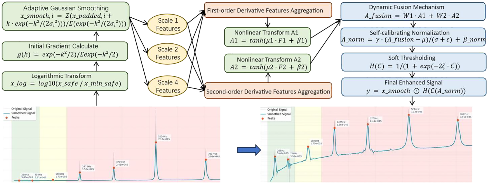
Logarithmic frequency dual attention signal processing method flowchart.

First, to stabilize variance and normalize the input data, the module performs logarithmic transformation on the input signal. Given an input tensor x with shape (B, C, L), where B is the batch size, C is the number of channels, and L is the signal length. The mathematical expression for logarithmic transformation is

x_{\log} = \log_{10} (\frac{x_{safe}}{x_{\min, safe}})

(1)

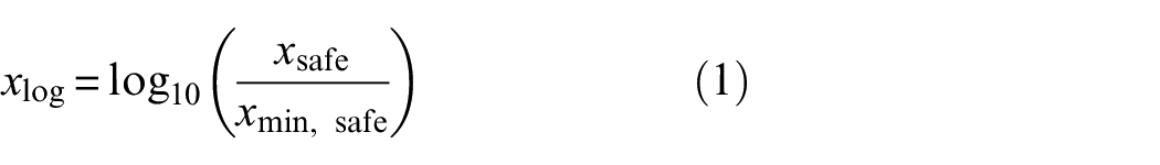
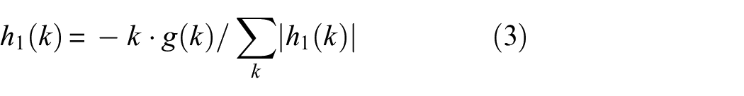
where $x_{\log}$ represents the signal after logarithmic transformation, $x_{safe} = \max (x, ϵ)$ , $x_{\min, safe} = \max (\min (x), ϵ / 2, 1)$ , $ϵ = 1 \times 10^{- 7}$ is a threshold parameter to ensure numerical stability. This transformation effectively compresses the dynamic range of the signal while maintaining the relative relationships of the signal.

After logarithmic transformation, the first-order variation characteristics of the signal are captured by calculating the initial gradient. The initial gradient is obtained through convolution with a first-order derivative kernel:

g_{initial} = x_{\log} * h_{1}

(2)

where the first-order derivative kernel $h_{1}$ is defined as follows:

h_{1} (k) = - k \cdot g (k) / \sum_{k} | h_{1} (k) |

(3)

The expression for Gaussian kernel $g (k)$ is

g (k) = \exp (- \frac{k^{2}}{2}) / \sum_{k} \exp (- \frac{k^{2}}{2})

(4)

Based on initial gradients, the module implements adaptive Gaussian smoothing. The smoothing intensity is dynamically adjusted through local gradients, preserving more details in areas of dramatic signal changes while applying stronger smoothing in flat regions. The formula for calculating the adaptive standard deviation is

σ_{i} = \frac{σ_{0}}{1 + λ_{adapt} \cdot | g_{initial, i} |}

(5)

smoothing operation expression is

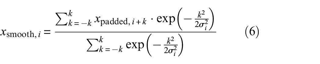
x_{smooth, i} = \frac{\sum_{k = - k}^{k} x_{padded, i + k} \cdot \exp (- \frac{k^{2}}{2 σ_{i}^{2}})}{\sum_{k = - k}^{k} \exp (- \frac{k^{2}}{2 σ_{i}^{2}})}

(6)

where $σ_{0}$ is the baseline standard deviation (initial value 2.0), $λ_{adapt}$ controls the sensitivity of smoothing to gradients (initial value 8.0).

To capture features at multiple resolutions, the module extracts first-order and second-order derivative features at different scales. For each scale $s \in 1, 2, 4,$ the feature extraction process is

g_{s}^{(1)} = x_{smooth}^{(s)} * h_{1}

(7)

g_{s}^{(2)} = g_{s}^{(1)} * h_{1}

(8)

multiscale features are aggregated through learnable weights:

F_{n} = \sum_{s} w_{s, n} \cdot g_{s}^{(1)}

(9)

where $w_{s, n}$ represents learnable weight parameters that adjust the contribution of features at different scales s; n denotes the feature channel index; $F_{n}$ represents the aggregated features for the nth channel. Aggregated derivative features then undergo nonlinear transformation to introduce stronger expressive capabilities:

A_{n} = \tan h (μ_{n} \cdot F_{n} + β_{n})

(10)

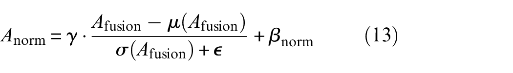
where μ, β are learnable parameters.

To effectively fuse dual attention maps, the module employs a dynamic fusion mechanism:

W = Softmax (F \cdot K)

(11)

A_{fusion} = W_{1} \cdot A_{1} + W_{2} \cdot A_{2}

(12)

where $K \in R^{C \times L}$ represents the convolution layer weight matrix of the fusion network, $C$ is the number of feature channels, and $L$ is the signal length; $W$ represents the attention weight matrix. where F represents the concatenation of attention maps, and K represents the convolution layer weights of the fusion network.

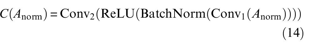
The fused attention map undergoes self-calibrating normalization:

A_{norm} = γ \cdot \frac{A_{fusion} - μ (A_{fusion})}{σ (A_{fusion}) + ϵ} + β_{norm}

(13)

where $γ$ and $β_{norm}$ are learnable scaling and bias parameters for adaptive feature distribution adjustment; $μ (\cdot)$ and $σ (\cdot)$ represent mean and standard deviation calculation operations, respectively.

C (A_{norm}) = Con v_{2} (ReLU (BatchNorm (Con v_{1} (A_{norm}))))

(14)

Finally, introduce a soft threshold mechanism through a smoothed Heaviside function:

H (C) = \frac{1}{1 + \exp (- 2 ζ \cdot C)}

(15)

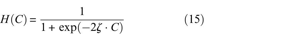
where ζ is a learnable parameter that controls the steepness of the transition. The final enhanced signal is obtained through the following method:

y = x_{smooth} ⊙ H (C (A_{norm}))

(16)

where ⊙ denotes elementwise multiplication operation.

At the implementation level, the logarithmic frequency dual attention module is built based on PyTorch’s nn.Module. All learnable parameters, including $σ_{0}$ , $λ_{adapt}$ , feature weights, $μ$ , $β$ , $γ$ , $β_{norm}$ and $ζ$ , are initialized as trainable nn.Parameter tensors. The Gaussian kernel and derivative kernel are registered as buffers through the register_buffer method during module instantiation, ensuring they remain constant during training. This design guarantees both computational efficiency and numerical stability.

Through the careful design and organic integration of the above components, the logarithmic frequency dual attention module achieves effective enhancement of input signals. This module not only adaptively adjusts processing intensity but also captures signal features at multiple scales, providing a reliable foundation for subsequent signal processing tasks.

Bidirectional-attention multistage fusion network

Network framework

In the field of signal processing, the effective processing and fusion of multichannel signals has consistently been a key area of research. Traditional methods often adopt a single fusion strategy, making it difficult to fully utilize feature information from different levels. To address this issue, this study proposes a new network architecture that enhances model performance through multistage attention feature fusion. The network employs a progressive feature extraction strategy and introduces attention mechanisms at different levels for feature fusion, effectively improving feature utilization efficiency. The proposed network architecture is shown in Figure 3, which extracts features through multilayer convolutional neural networks (CNN) and achieves effective feature fusion using bilateral attention fusion modules (BFM). The following sections will provide a detailed description of each component of the network, along with its mathematical formulation.

Figure 3.

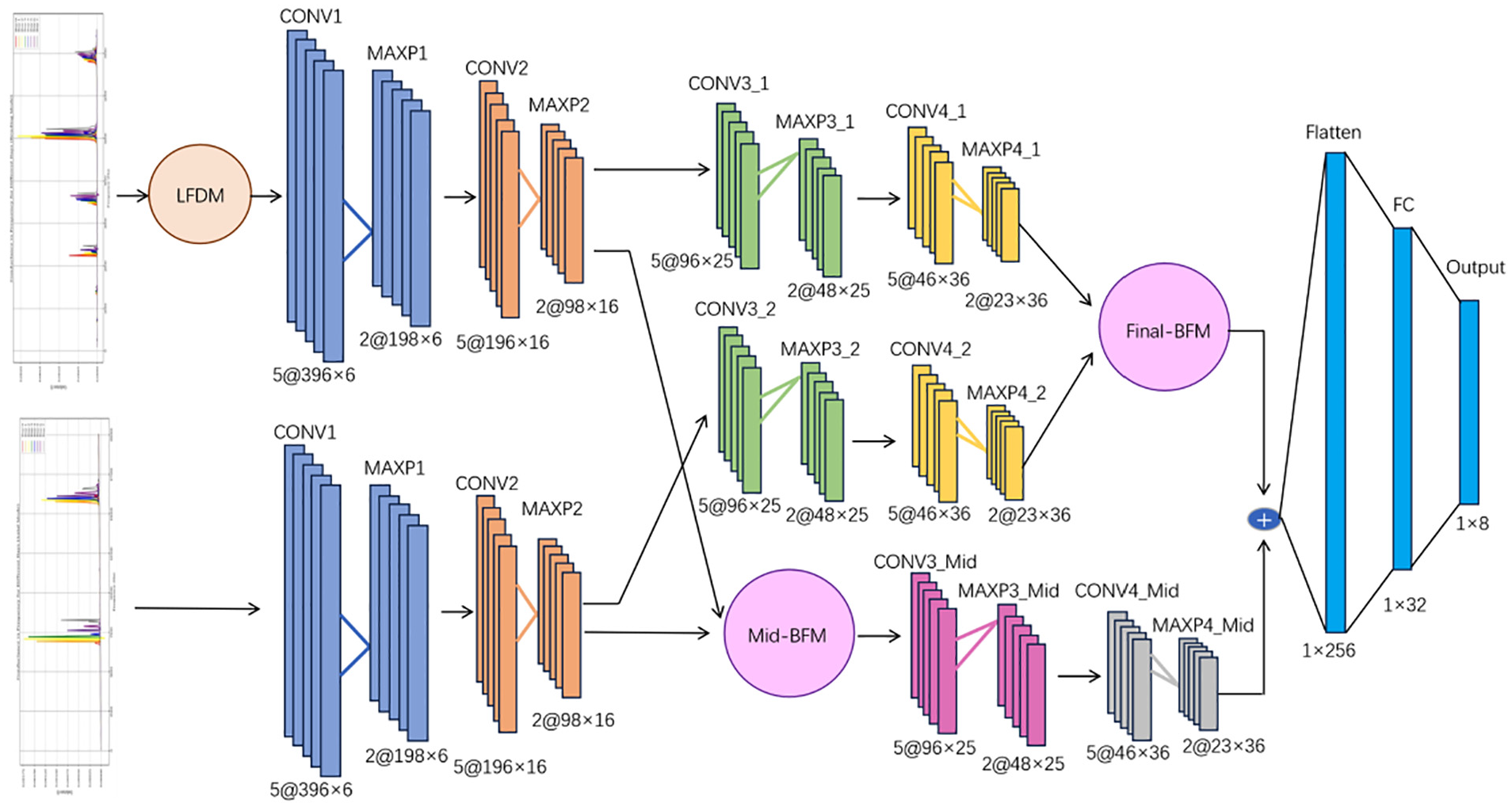
Bidirectional multilevel fusion network structure.

The overall network consists of logarithmic frequency dual attention module, feature extraction layers (including multiple convolution, batch normalization, pooling, and activation function layers), a middle fusion module (Mid-BFM), a final fusion module (Final-BFM), and fully connected layers (FC). The network receives two input signals ( $x_{1}$ ) and ( $x_{2}$ ), extracts features through a series of convolutional layers, fuses features from different paths through fusion modules, and finally outputs classification results through fully connected layers.

Before the input signal enters the feature extraction layer, it first undergoes preprocessing through the logarithmic frequency dual attention module, which is a logarithmic frequency domain dual attention mechanism, to enhance the expression of important features. Let the input signal be (x), and the output after the attention mechanism is: $x^{'} = Attention (x)$ , where $(Attention (\cdot))$ represents the computational process of the attention mechanism. The feature extraction part consists of multiple convolutional network layers, each including convolution operations, batch normalization, pooling, and activation functions. For the two input signals $(x_{1})$ and $(x_{2})$ , preliminary feature extraction is performed through two parallel convolutional branches:

\begin{matrix} h_{1} (t) = ReLU (MaxPool 1 d (BatchNorm 1 d (Conv 1 d \\ (x; 1 \to 6, K = 5, S = 1)))) \end{matrix}

(17)

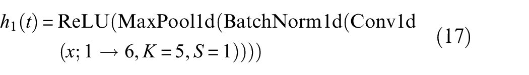
Parameters for Conv1d operations: $K$ represents kernel size, $S$ represents stride, input, and output channels are indicated by arrows (e.g., 1 → 6 indicates mapping from 1 input channel to 6 output channels). All convolution layers use the same padding strategy with “same” padding to maintain sequence length. Where $Conv 1 d (x; in_channels \to out_channels, K, S)$ represents a one-dimensional convolution operation, with parameters of kernel size (K=5), stride (S=1), and output channels of 6.

Continues to perform convolution processing on the features output from the first layer to extract higher-level features:

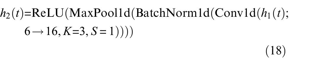
\begin{matrix} h_{2} (t) = ReLU (MaxPool 1 d (BatchNorm 1 d (Conv 1 d (h_{1} (t); \\ 6 \to 16, K = 3, S = 1)))) \end{matrix}

(18)

Here, $Conv 1 d$ uses a kernel size of K = 3, stride S = 1, and increases the output channels to 16.

The features extracted from the second layer are fused through the intermediate fusion module BFM:

h_{mid} = BFM (h_{2} (t_{1}), h_{2} (t_{2}))

(19)

Subsequently, the fused features undergo further processing through convolutional layers:

\begin{matrix} h_{3} (mid) = ReLU (MaxPool 1 d (BatchNorm 1 d \\ (Conv 1 d (h_{mid}; 16 \to 25, K = 3, S = 1)))) \end{matrix}

(20)

\begin{matrix} h_{4} (mid) = ReLU (MaxPool 1 d (BatchNorm 1 d \\ (Conv 1 d (h_{3 mid}; 25 \to 36, K = 3, S = 1)))) \end{matrix}

(21)

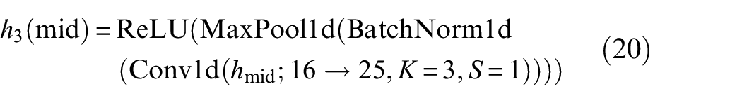
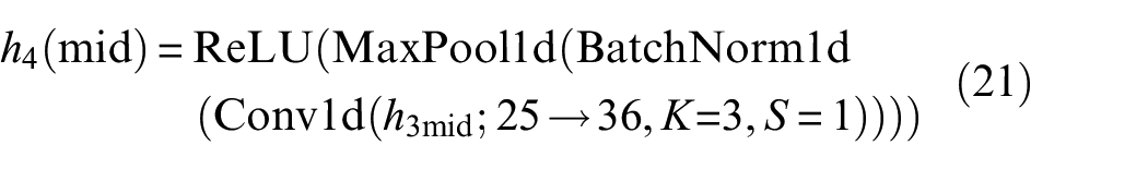
Among them, Conv1d increases the number of channels from 16 to 25, and then to 36.

Outside the middle-layer fusion branch, the original feature branch continues to propagate forward, going through the third and fourth convolutional layers:

\begin{matrix} h_{3} (t) = ReLU (MaxPool 1 d (BatchNorm 1 d (Conv 1 d (h_{2} (t); \\ 16 \to 25, K = 3, S = 1)))) \end{matrix}

(22)

\begin{matrix} h_{4} (t) = ReLU (MaxPool 1 d (BatchNorm 1 d (Conv 1 d (h_{3} (t); \\ 25 \to 36, K = 3, S = 1)))) \end{matrix}

(23)

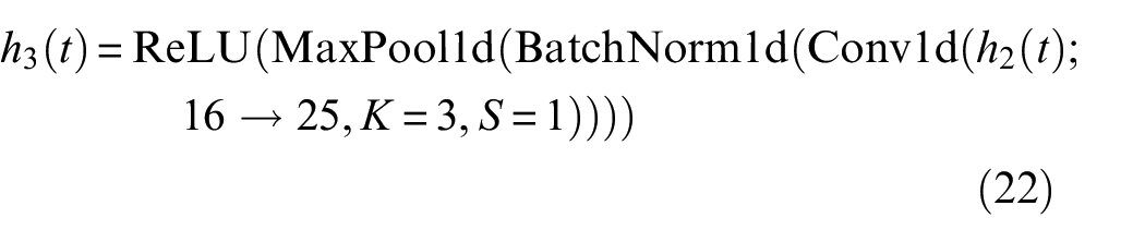
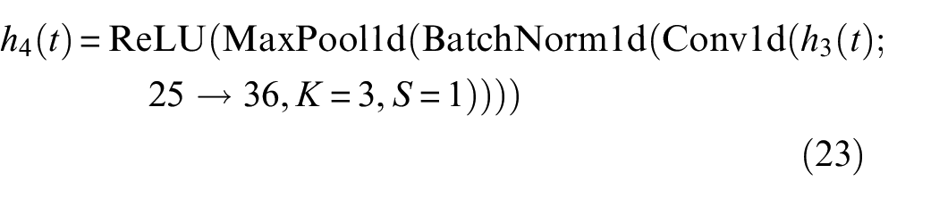
Here, Conv1d increases the number of channels from 25 to 36.

Fuses the fourth layer features of the original branch through the final fusion module BFM:

h_{final} = BFM (h_{4} (t_{1}), h_{4} (t_{2}))

(24)

Next, use the weighted fusion mechanism to combine the features of middle-layer fusion and final fusion: $α = σ (w)$ where w is the fusion weight parameter $h_{fused} = α \cdot h_{final} + (1 - α) \cdot h_{mid}$ , where $σ (\cdot)$ represents the Sigmoid function, ensuring the fusion weight $α$ is between 0 and 1.Finally, flatten the fused features and perform classification through fully connected layers.

In summary, the network proposed in this study adopts an innovative two-stage feature fusion strategy. The first stage performs intermediate feature fusion after the second convolutional layer, and the fused features continue through their respective processing branches. The second stage performs final feature fusion after the fourth convolutional layer to obtain more comprehensive feature representation.

First-stage feature fusion: After completing the initial parallel feature extraction, the network implements a novel bidirectional attention fusion mechanism to integrate feature signals from both branches at the intermediate level. This early fusion strategy is designed to timely integrate multisource information and prevent effective features from degrading in deeper networks. The fused features continue through two consecutive convolutional layers, with channels progressively expanding to 25 and 36, forming a mid-level fusion branch. This progressive channel expansion strategy ensures sufficient feature extraction while avoiding excessive computational resource consumption.

Second stage feature fusion: After the first stage fusion strategy, the mid-level fusion branch proceeds in parallel with the continuous extraction of original features. The two original branches continue to be processed through convolutional networks with identical structures, maintaining a channel expansion strategy (16 → 25 → 36) consistent with the mid-level fusion branch. This symmetrical design not only maintains the consistency of feature extraction but also provides a solid foundation for subsequent feature fusion. Each convolutional layer is still equipped with complete Batch Norm, MaxPool, and ReLU components, ensuring effective extraction of deep features. A bidirectional attention fusion mechanism is similarly designed at the network’s end for deep feature fusion.

This network architecture offers several technical advantages: first, the multistage fusion strategy effectively leverages feature information across different scales; second, the adaptive fusion mechanism dynamically adjusts the importance of each fusion stage using learnable parameters; third, the hook mechanism allows for efficient monitoring of key node features, facilitating network analysis and debugging; and finally, the bidirectional symmetric structure ensures balanced processing of input signals.

Bidirectional-attention fusion module

While attention mechanisms have demonstrated remarkable success in various deep learning tasks, limitations still exist when dealing with one-dimensional convolutional neural networks. SE-Net²⁹ pioneered the channel attention mechanism by explicitly modeling interdependencies between channels: first compressing global spatial information into channel descriptors, then activating these descriptors to recalibrate channel feature responses. However, SE-Net only focuses on channel relationships, ignoring temporal dependencies in one-dimensional sequential data. CBAM³⁰ expanded the application of attention mechanisms by serially integrating channel and spatial attention modules. Although CBAM achieved impressive performance in two-dimensional image processing tasks, its spatial attention module was designed specifically for 2D feature maps and cannot be directly applied to one-dimensional sequential data without significant modifications. Temporal attention emphasizes the importance of temporal information in sequential data by capturing dependencies along the time dimension, while effective in modeling temporal relationships, it neglects channel correlations that could provide complementary feature representations. Coordinate attention³¹ proposed a position-sensitive attention mechanism that preserves precise position information in 2D images and effectively captures channel and spatial dependencies, but its design is specifically optimized for two-dimensional scenarios and cannot be directly applied to one-dimensional sequence data processing.

To address the limitations of existing attention mechanisms in processing one-dimensional sequence data, a BFM is proposed, which can simultaneously model channel and temporal dependencies in one-dimensional convolutional neural networks. Compared to existing methods, BFM has significant advantages: unlike SE-Net which only focuses on single-dimensional attention, unlike CBAM and coordinate attention which require two-dimensional input, and unlike temporal attention which ignores channel relationships. BFM adopts a bidirectional parallel structure to simultaneously capture channel relationships and temporal dependencies, providing more comprehensive feature representation for one-dimensional sequence data.

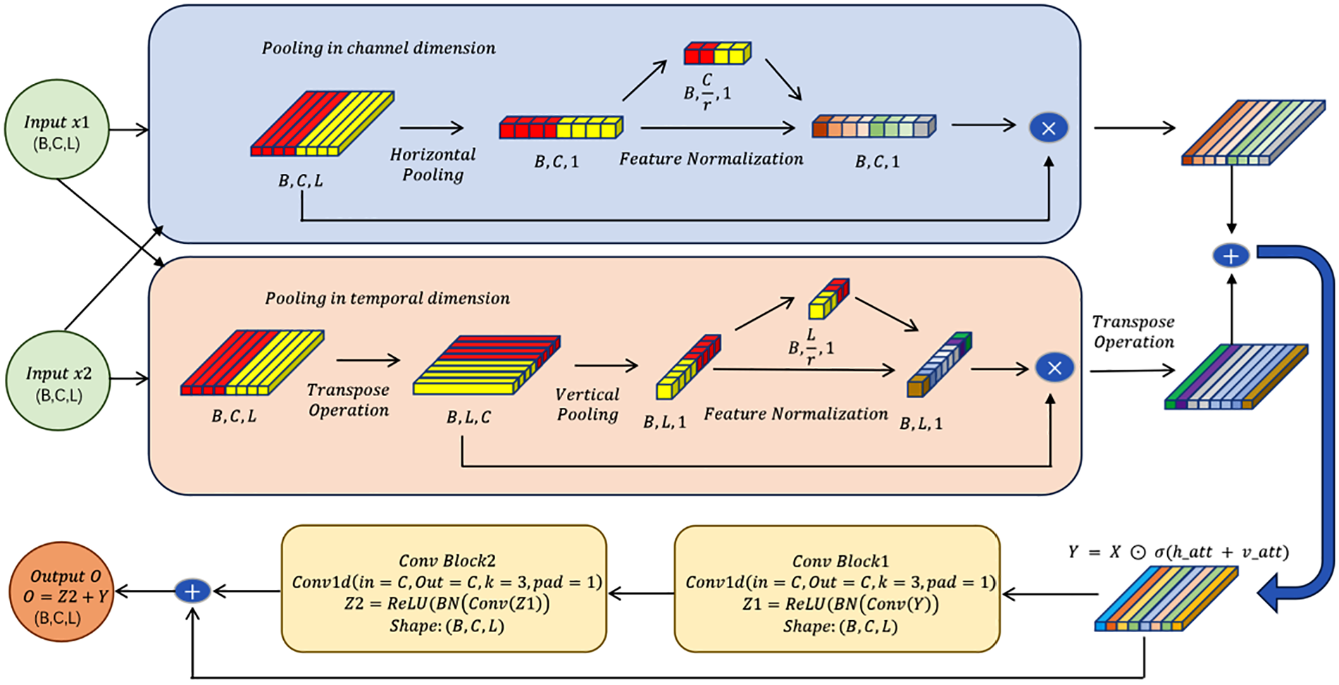
Based on a thorough understanding of the limitations of existing attention mechanisms, the proposed BFM not only innovatively achieves parallel computation of bidirectional attention, but more importantly introduces a feature fusion mechanism. BFM adopts a modular design as shown in Figure 4. Specifically, BFM contains two key innovations: first, it calculates channel attention and temporal attention separately through a parallel dual-branch structure, avoiding potential information loss from traditional serial structures; second, it employs an additive fusion mechanism to merge enhanced features with original features, effectively enhancing features while preserving original feature information through residual connections.

Figure 4.

Bidirectional-attention fusion module architecture diagram.

From a mathematical perspective, the dual-branch structure can be viewed as an orthogonal decomposition of the feature space, which decomposes the original feature map $X \in R^{C \times L}$ into the product of channel attention and temporal attention. This orthogonal decomposition has three main advantages: reducing feature dimension coupling, enhancing feature representation capability, and decreasing computational overhead. Compared to computing global attention simultaneously in both channel and temporal dimensions, the computational complexity of the dual-branch structure is reduced from $O (C \times L)$ to $O (C + L)$ , significantly improving computational efficiency. In the specific implementation, given two input feature maps from different modalities, denoted as $T_{1}$ and $T_{2} \in R^{C \times L}$ , where C is the number of channels and L is the temporal length, they are first fused through averaging:

X = \frac{T_{1} + T_{2}}{2}

(25)

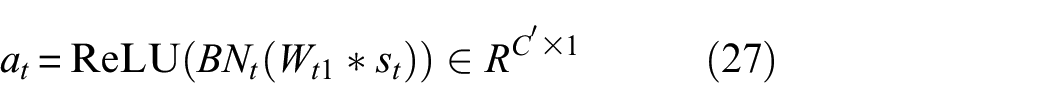
applies global average pooling along the temporal dimension first to capture temporal dependencies:

s_{t} = {AvgPool}_{L} (X) = \frac{1}{L} \sum_{i = 1}^{L} X_{:, i} \in R^{C}

(26)

Here, $X_{:, i}$ represents the i-th time slice of X.

Then, pass $s_{t}$ through two bottleneck layers with convolution layers of reduction ratio r, batch normalization, and ReLU activation:

a_{t} = ReLU (B N_{t} (W_{t 1} * s_{t})) \in R^{C^{'} \times 1}

(27)

b_{t} = W_{t 2} * a_{t} \in R^{C \times 1}

(28)

where $C^{'} = \frac{C}{r}$ is the reduced channel dimension, * represents convolution with kernel size 1, $W_{t 1} \in R^{C^{'} \times C}$ and $W_{t 2} \in R^{C \times C^{'}}$ are convolution weights, $B N_{t}$ is the batch normalization for temporal attention.

Adopts a similar approach in channel-dependent processing, first applying global average pooling along the channel dimension. Since the standard 1D convolution layer in PyTorch does not directly support pooling along the channel dimension, this process is simulated by transposing the dimensions of X:

\tilde{X} = X^{T} \in R^{L \times C}

(29)

applies global average pooling along the new temporal dimension (original channel dimension):

s_{c} = {AvgPool}_{C} (\tilde{X}) = \frac{1}{C} \sum_{j = 1}^{C} \tilde{X_{:, j}} \in R^{L}

(30)

reshapes $s_{c}$ into $R^{1 \times L}$ , then through a similar bottleneck:

a_{c} = ReLU (B N_{c} (W_{c 1} * s_{c})) \in R^{C^{'} \times 1}

(31)

b_{c} = W_{c 2} * a_{c} \in R^{C \times 1}

(32)

where $W_{c 1} \in R^{C^{'} \times 1}$ and $W_{c 2} \in R^{1 \times C^{'}}$ are convolution weights, $B N_{c}$ is the batch normalization for channel attention.

Next, the attention map is generated by integrating temporal and channel attention features, followed by the application of the Sigmoid activation function:

A = σ (b_{t} + b_{c}) \in R^{C \times 1}

(33)

where σ represents the element-wise Sigmoid function.

After obtaining the attention map, it is applied to the features. The attention map A is expanded to match the dimensions of the input feature map and is applied to the fused features:

Y = (T_{1} + T_{2}) ⊙ A

(34)

where ⊙ represents elementwise multiplication, and A is broadcast along the temporal dimension to match the shape of $T_{1} + T_{2}$ .

To further enhance the discriminative ability of features, a convolutional refinement process with residual connections is introduced. The feature map Y processed by the attention mechanism first goes through the initial convolution block, applying 1D convolution with a kernel size of 3, followed by batch normalization and ReLU activation:

Z_{1} = {ReLU (BN}_{1} ({Conv}_{1 D} (Y)))

(35)

where ${Conv}_{1 D}$ is the 1D convolution operation, and $B N_{1}$ is the batch normalization layer of the first convolution block.

Immediately applies the second convolution block in a similar way:

Z_{2} = ReLU ({BN}_{2} ({Conv}_{1 D} (Z_{1})))

(36)

where $B N_{2}$ is the batch normalization layer of the second convolution block.

Finally, to promote gradient flow and improve training stability, the attention-applied features Y are added to the output of the second convolutional block to form a residual connection:

O = Z_{2} + Y

(37)

This residual addition helps the network learn identity mapping, making it easier to optimize. In this way, the output O represents the optimized feature map, which effectively combines information from both modalities while emphasizing discriminative features through the coordinate attention mechanism.

In summary, this mechanism receives two input feature sequences (both with dimensions B×C×L, where B is batch size, C is number of channels, and L is sequence length), and processes them in parallel through two paths. In the channel attention branch, average operation is used along the channel dimension for feature aggregation to obtain correlation information between channels; in the temporal attention branch, adaptive average pooling compresses the temporal dimension to unit length, generating compact temporal feature descriptions. The features from these two branches are concatenated and transformed through two stages of convolutional neural networks. The first convolutional layer, coupled with batch normalization and ReLU activation function, performs feature dimensionality reduction, with the temporal branch compressing C channels to C/r and the channel branch compressing 2 feature maps to L/r (where r is the compression ratio). The second convolutional layer remaps the features to their original dimensions and generates attention weight maps through a Sigmoid function. This design based on learnable convolutional layers enables the model to adaptively adjust feature weights in different dimensions, thereby highlighting important temporal patterns and channel features.

Experimental verification

Experimental specimen and instrument setup

Three electrochemical corrosion probes were fabricated in Hubei key laboratory of earthquake early warning, with dimensions shown in Figure 5. The probes are labeled as No. 1, No. 2, and No. 3. These probes were manufactured using high-purity aluminum to ensure material consistency and experimental reliability. Each probe measures 236 mm (length) × 26 mm (width) × 4 mm (thickness), designed to simulate common corrosion environments. An aluminum cubic mass block measuring 29 × 29 × 29 mm was welded to the end of each probe, which not only enhanced the mechanical stability of the probe but also helped simulate stress distribution under actual working conditions. The mass block was made of the same aluminum material as the probe body to avoid electrochemical performance inconsistencies due to material differences.

Figure 5.

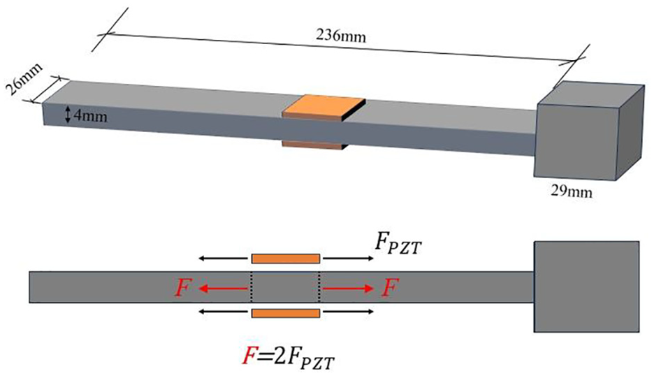
Corrosion probe schematic diagram.

PZT-5H piezoelectric sensors with dimensions of 20 × 20 × 0.5 mm were installed on both the front and back sides at the center of the probe. Highly conductive epoxy resin was applied to the surface of the probe, extending 1 mm beyond the piezoelectric sheet to ensure optimal electrical signal transmission and mechanical coupling. This setup was used to monitor conductance changes during the corrosion process. The sensor was installed at the center of the probe to ensure that the changes in the conductance signal could be accurately captured at different corrosion stages. The conductance measurement system of the experiment mainly consists of an impedance analyzer, a data acquisition system, and a computer, as shown in Figure 6. The impedance analyzer used in the experiment was the WAYNE KERR 6500B, which accurately measured the conductance signal of the probe under varying corrosion conditions. The subsequent processing was completed by a computer equipped with an Intel Core i7 processor (Intel Corporation, Santa Clara, California, USA) and 16 GB of memory.

Figure 6.

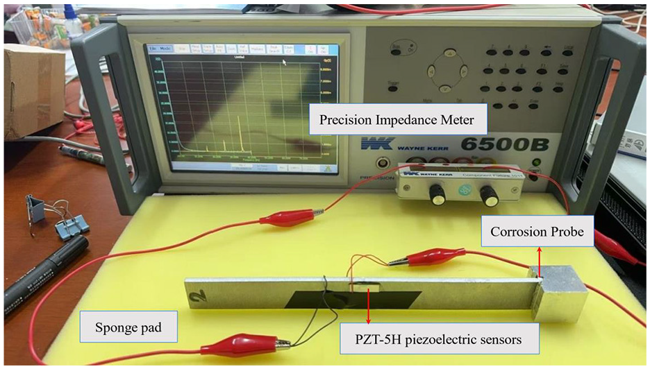
Experimental specimen and instrument setup.

During the measurement of conductance signals, specific circuit connection methods were employed to collect signals from both axial and bending vibration modes. The specific connection methods are shown in Figure 7. For the axial vibration mode, lead 1 of both piezoelectric sensors (PZT-A and PZT-B) are connected to terminal 1 of the impedance analyzer, while both lead 2 are connected to terminal 2. For the bending vibration mode, as shown in Figure 7(b), the connections are reversed: lead 1 of PZT-A and lead 2 of PZT-B are connected to terminal 1, while lead 1 of PZT-B and lead 2 of PZT-A are connected to terminal 2. This bidirectional connection method effectively measures conductance signals in both axial and bending modes, ensuring the accuracy and reliability of signal acquisition.

Figure 7.

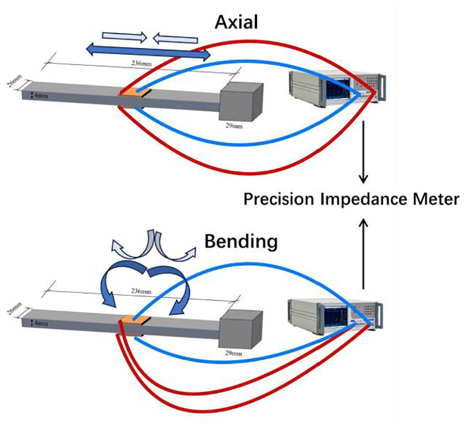
(a) Axial mode: similar leads are connected together and (b) Bending mode: leads are interchanged before connection.

Experimental procedure

The objective of this study is to evaluate the performance of aluminum probes No. 1, No. 2, and No. 3 through accelerated corrosion tests conducted in real-world corrosive environments. To ensure experimental reproducibility and data accuracy, the experimental environment was strictly controlled at a constant temperature of 26°C and 60% relative humidity, with an air conditioning system maintaining stable indoor temperature. The corrosive medium used was 3.5% sodium chloride (NaCl) solution to simulate corrosive conditions in marine environments. During the experimental preparation phase, all probes were subjected to a surface cleaning procedure. Ethanol was employed to remove contaminants and oxide layers from the surfaces. Additionally, special attention was given to securing the welding points of the aluminum cubic mass blocks to prevent mechanical loosening throughout the subsequent corrosion process. After sensor installation, careful inspection of connections was required to avoid signal loss during data acquisition. According to different connection methods for axial and bending modes, the impedance analyzer was connected to the sensors, ensuring good contact at all connection terminals. To guarantee measurement accuracy, all instruments and equipment underwent strict calibration before the experiment. The impedance analyzer was zero-calibrated before each experiment, and the data acquisition system was verified using standard signal sources.

The design of the accelerated corrosion test apparatus is illustrated in Figure 8. In this setup, the aluminum probe functions as the anode and is connected to the positive terminal of the DC power supply. The copper plate serves as the cathode and is connected to the negative terminal of the power supply. To ensure uniform corrosion process, the third section of the probe is immersed in 3.5% NaCl solution along with the copper plate. During the accelerated corrosion process, a constant current of 620 mA is applied to accelerate the corrosion rate of the aluminum probe. This current setting was specifically chosen to achieve a controlled corrosion rate of 5 g mass loss per day, which serves as our basic classification unit for corrosion progression (Day 0 corresponding to 0 g mass loss, Day 1 to 5 g, Day 2 to 10 g, and so forth). According to Faraday’s law, the relationship between mass loss Δm and applied current I, time t, charge number of aluminum ions z, and Faraday’s constant F is

Δ m = \frac{M \cdot I \cdot t}{z \cdot F}

(38)

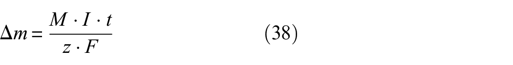
where M is the atomic mass of aluminum (27 g/mol), z is the charge number of aluminum ions (z = 3), and F is the Faraday constant (96,485 C/mol). The expected daily mass loss is approximately 5 g. The entire test process lasted for 8 days, and the experiment was conducted under constant room temperature conditions to ensure consistency and reproducibility of the experimental environment.

Figure 8.

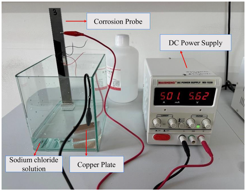
Accelerated corrosion test device diagram:

During the experiment, impedance spectroscopy measurements of each probe were conducted at regular times daily, and mass loss data were recorded. The specific procedure was at the same time each day, the current supply was stopped, and an impedance analyzer was used to record the conductance characteristics of the probes in their current corrosion state, obtaining conductance data in two modalities. Meanwhile, a precision balance was used to measure the mass loss of each probe, ensuring data accuracy through multiple measurements and calibrations. All daily impedance spectra and mass loss data were recorded and saved, forming a systematic time series database. During the data processing and analysis phase, the collected impedance spectra and mass loss data were transferred to a computer for analyzing the trends of impedance spectra over corrosion time, exploring the relationship between conductance characteristics and corrosion degree, providing a basis for multimodal fusion analysis. During the experiment, regular checks of connection circuits and sensor status were necessary to promptly identify and eliminate potential faults, ensuring smooth experimental progress.

Through the optimized experimental process above, rich corrosion data could be obtained in a relatively short time, verifying the performance of aluminum probes in actual corrosive environments. This not only provided a solid data foundation for subsequent corrosion behavior analysis but also offered practical support for the application of multimodal fusion technology in corrosion monitoring.

Frequency response characteristics analysis and frequency domain selection

The analysis of the first two resonance peaks in the axial mode is shown in Figure 9, where the main resonance frequencies of Day 0 are marked in the figure. Through detailed analysis of the conductance-frequency curve, two significant resonance characteristics can be observed. The first resonance peak appears at approximately 7500 Hz, which is the most significant resonance response region, with a maximum conductance value of about 0.00175 Siemens (S). This resonance peak exhibits very sharp characteristics, indicating highly concentrated energy at this frequency point, particularly prominent on the second and third days of the experiment. Notably, the amplitude of this resonance peak shows certain variation trends as experimental days progress, which may be related to the degree of material corrosion. The second resonance peak is located in the high-frequency region at approximately 16,000 Hz, and although its amplitude is relatively smaller, about 0.0013 Siemens, it still shows clear resonance characteristics. This high-frequency resonance peak demonstrates good consistency across different test dates, with clearly distinguishable peak shapes, indicating that the structural response at this frequency has good reproducibility and stability. In the frequency range between the two resonance peaks, the conductance curve appears relatively smooth, maintaining at a relatively low level, indicating no significant resonance phenomena occur in these frequency ranges.

Figure 9.

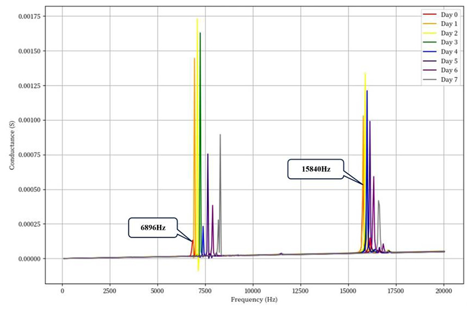
Axial mode conductance curve.

The analysis of the first seven resonance peaks in the bending mode is shown in Figure 10, where the main resonance frequencies of Day 0 are marked in the figure. The first resonance peak appears at approximately 300 Hz, representing the fundamental bending vibration mode of the structure. Its amplitude is relatively small and shows good stability across all test samples. The second resonance peak is located at approximately 700Hz, corresponding to the second-order bending vibration of the structure, with concentrated energy distribution but still lower amplitude than the peaks in the high-frequency region. The third resonance peak at approximately 1500 Hz exhibits moderate resonance response, with a narrow and clear peak shape and good response consistency across test dates. The fourth resonance peak is located at approximately 2500 Hz, showing strong resonance characteristics with peak amplitude significantly higher than the low-frequency band and stable performance across different test dates. The fifth resonance peak appears in the high-frequency band at approximately 3800 Hz, serving as a significant characteristic peak with concentrated energy and distinct peak values, showing moderate response intensity. The sixth resonance peak is located at approximately 5000 Hz, representing the strongest resonance response area with maximum peak amplitude and good reproducibility across test dates. Finally, the seventh resonance peak appears in the highest frequency band at approximately 6500–7000 Hz, maintaining stability despite relatively low energy, with clearly distinguishable peak values reflecting the structure’s response characteristics under high-frequency excitation.

Figure 10.

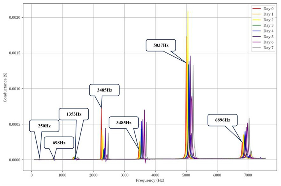
Bending mode conductance curve.

Through analysis of experimental data, the optimal acquisition parameters and frequency ranges were determined. For the axial mode, a frequency range of 100 Hz to 20 kHz was selected, containing two main resonance peaks with significant signal characteristics and good data repeatability, collecting 400 data points for each condition. For the bending mode, a frequency range of 100 Hz to 7.5 kHz was selected, covering seven characteristic resonance peaks, providing rich frequency response information, with 400 data points collected for each condition as well. During the experiment, the conductance signals of both axial and bending modes were collected independently to facilitate subsequent multimodal fusion analysis.

Result analysis

Logarithmic frequency dual attention module result analysis

This study validates the effectiveness of the proposed model through systematic experimental design and comprehensive data analysis. The experiments were conducted under the PyTorch framework, with the network accepting input data of dimension (batch_size, 1, 400). Through layer-by-layer feature extraction, the intermediate feature dimensions were 6, 16, 25, and 36 successively, ultimately outputting prediction results for eight categories. The dataset was randomly divided into training and test sets at an 80:20 ratio. During training, SGD optimizer with momentum was used for parameter optimization, with a learning rate of 0.0015, momentum factor of 0.9, and CrossEntropyLoss as the loss function. Training was conducted for five epochs, with a batch size of 16 for training and four for testing to balance computational efficiency and model performance. To monitor the training process, the system recorded changes in loss values and accuracy during both training and testing, presenting them through visualization. To verify the performance and stability of the proposed model, this study conducted 10 independent training experiments on the axial vibration mode recognition model, with results shown in Figure 11. The model achieved accuracies of 82.5%, 96.63%, 92.38%, 88.88%, 66.63%, 81.88%, 79.13%, 66.88%, 83.00%, and 82.5% across the 10 training runs, with an average accuracy of 82.04%. The highest accuracy was 96.63%, the lowest was 66.63%, with a standard deviation of 9.47%. The experimental data shows that six experiments achieved accuracy above 80%, with three reaching over 90%, indicating that the model maintains good recognition performance in most cases and has the potential to achieve excellent performance.

Figure 11.

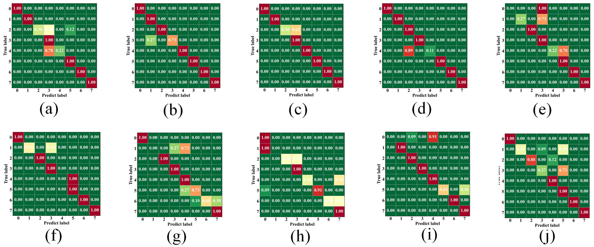
Axial mode training confusion matrix: (a)-(j) Confusion matrices for ten independent training runs.

From the perspective of model stability, there are five experimental results in the 80%–85% accuracy range, representing the model’s stability performance interval. Although the standard deviation of accuracy at 9.47% indicates some fluctuation in model performance, considering the randomness in deep learning model training (such as weight initialization, data shuffling, and other factors), this level of fluctuation is acceptable. Notably, the model maintains accuracy above 66% across multiple experiments, with a 30% occurrence rate of accuracy above 90%, further confirming the model’s good reliability and excellent performance potential.

In conclusion, the experimental results demonstrate that the proposed axial vibration mode recognition model has good application potential. Despite some performance fluctuations, its overall performance is stable and reliable. Through further optimization and improvement, the model’s recognition accuracy and stability are expected to improve significantly, providing more solid technical support for practical applications. However, when training for bending vibration modes using the same experimental setup and training process, as shown in Figure 12, the model failed to effectively fit the data, experiencing collapse during training and failing to converge to an ideal state. This indicates that the original model has significant limitations in processing bending vibration mode signal characteristics and struggles to capture key time–frequency features.

Figure 12.

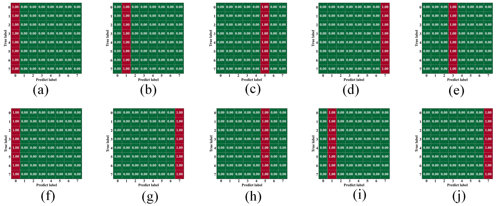
Bending mode training confusion matrix: (a)-(j) Confusion matrices for ten independent training runs.

To address this issue, logarithmic frequency dual attention module was introduced based on the original model. Figure 13 demonstrates the effectiveness of the proposed method in frequency response analysis. To comprehensively showcase the processing capability of the algorithm, both linear scale and logarithmic scale analysis results are presented. From the figure, it can be observed that the adaptive smoothing process (blue line) effectively preserves the main frequency characteristics of the original signal (gray line) while significantly suppressing noise effects. Particularly, under the logarithmic scale, the processing effects on low-amplitude signals can be observed more clearly.

Figure 13.

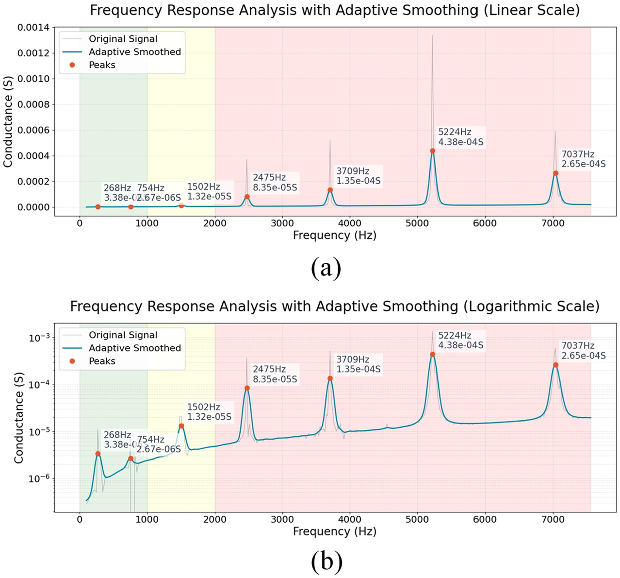
(a) Conductance curve in linear scale and (b) conductance curve in logarithmic scale.

Through analysis, it can be found that this method successfully identified and preserved seven main characteristic frequencies: 268, 754, 1502, 2475, 3709, 5224, and 7037 Hz. The amplitudes of these frequency components span multiple orders of magnitude, ranging from 10⁻⁶ to 10⁻³. In the linear scale spectrum shown in Figure 13(a), the processing effect of high-amplitude frequency components (such as the peak at 5224 Hz) can be intuitively observed, but low-amplitude frequency components are ignored. In contrast, in the logarithmic scale spectrum shown in Figure 13(b), not only is the high-amplitude information preserved, but the low-amplitude frequency components (such as peaks at 268 and 754 Hz) are also clearly displayed, achieving comprehensive visualization of both high- and low-amplitude frequency components.

The adaptive smoothing algorithm demonstrates excellent performance in frequency selectivity, not only significantly improving the signal-to-noise ratio while maintaining peak amplitudes but also effectively preserving the integrity of high-frequency components. For example, for the frequency component at 3709 Hz, the algorithm maintains the peak amplitude (1.35e-04S) while making the frequency response curve smoother and clearer. Similarly, for the high-frequency component at 7037 Hz (2.65e-04S), the algorithm also shows good processing capability. Notably, in the low-frequency band (0–1000 Hz) processing, the algorithm exhibits outstanding noise suppression ability. The logarithmic scale plot clearly shows that the algorithm successfully suppresses the surrounding background noise while preserving 2 weak signals at 268 Hz (3.38e-06S) and 754 Hz (2.67e-06S), an effect that is difficult to achieve with traditional linear smoothing methods.

By comparing the frequency response curves before and after processing, it is found that the peak position of the main frequency component remains unchanged, proving the phase retention characteristics of the algorithm; the frequency response between peaks is smoother, indicating that the background noise is effectively suppressed; signals of different amplitude levels are properly processed, reflecting the adaptive characteristics of the algorithm. These results fully demonstrate the effectiveness of the proposed adaptive smoothing algorithm in frequency domain processing, especially in achieving the key goal of noise suppression while maintaining signal characteristics. The addition of this module significantly improves the performance of the model, with an average accuracy of 92.5%. As shown in Figure 14, the introduction of logarithmic frequency dual attention module not only solves the problem that the original model cannot effectively fit the data but also significantly improves the model’s ability to recognize complex signals by integrating the adaptive attention mechanism of the first-order and second-order derivatives.

Figure 14.

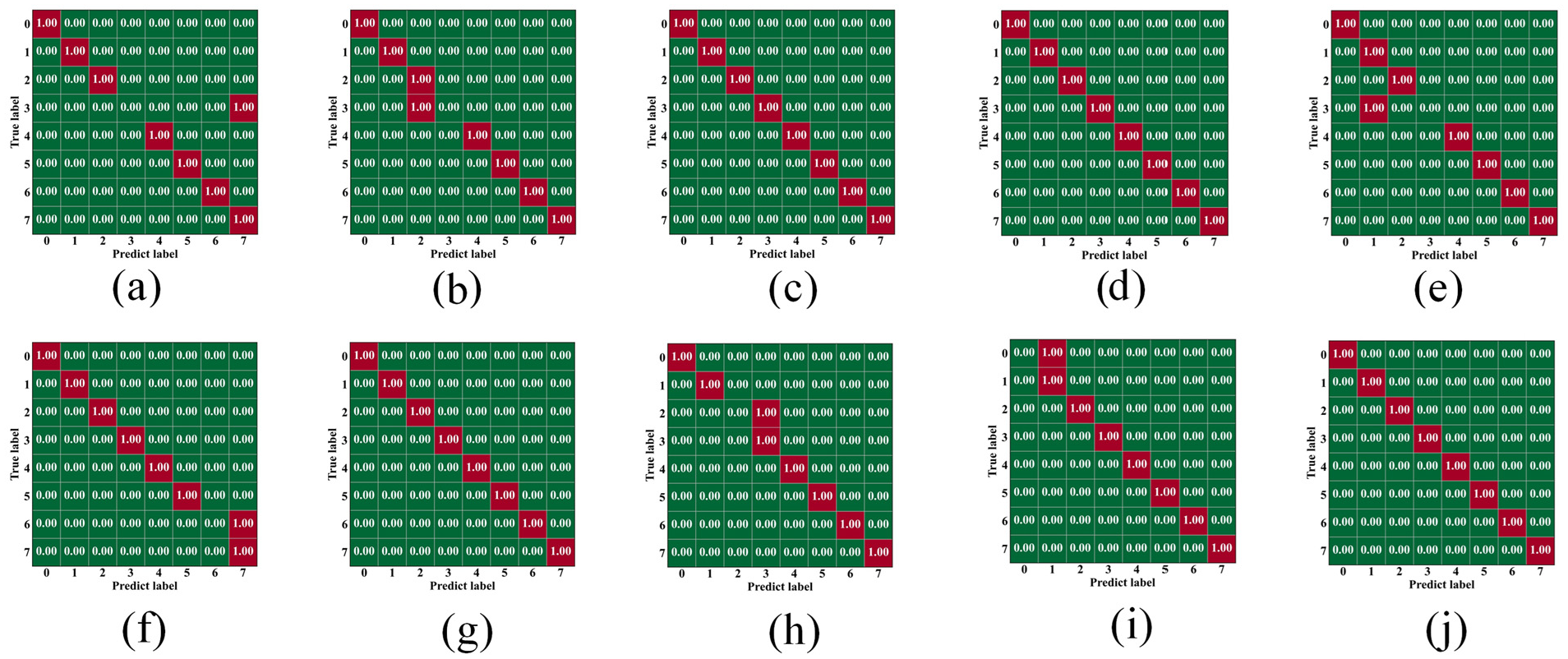
Logarithmic frequency dual attention module confusion matrix: (a)-(j) Confusion matrices for ten independent training runs.

Furthermore, to more intuitively demonstrate the role of the LFDM, a visualization analysis of the model’s attention weights was conducted. In Figure 15(a) is a logarithmic scale spectrum. The attention weight distribution based on first-order derivatives mainly captures the rate of change characteristics of signals as shown in Figure 15(b), presenting sharp peaks in the spectrum. The strongest attention response appears near 2500 Hz with a weight of 1.0, and the secondary peak is at 4000 Hz (weight approximately 0.9). However, these attention weights are unevenly distributed along the frequency axis, particularly in the low-frequency band (0–1000 Hz), where the weights are lower, limiting feature extraction capability. The attention weight distribution based on second-order derivatives reflects the curvature change characteristics of signals as shown in Figure 15(c), with attention weights showing discrete peaks in the spectrum. The strongest response is also near 2500 Hz, but the overall weight distribution lacks continuity, and the feature extraction capability in the high-frequency band is also limited.

Figure 15.

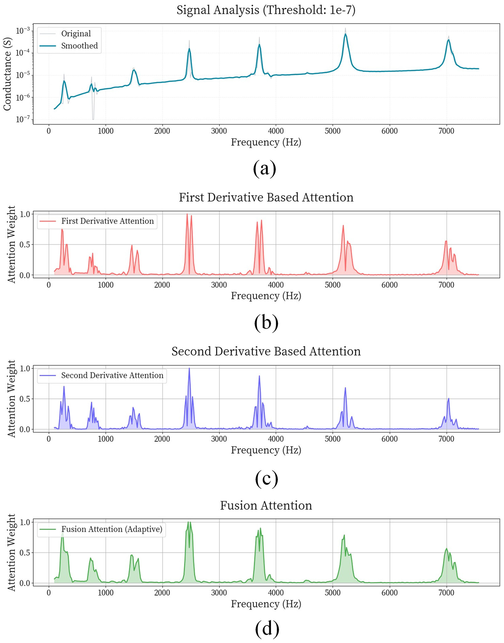
Frequency dual attention weight visualization analysis diagram: (a) Signal Ananlysis, (b) First Derivative Based Attention, (c) Second Derivative Based Attention, and (d) Fusion Attion.

In contrast, the adaptive fusion attention shown in Figure 15(d) combines the advantages of first-order and second-order derivatives in its weight distribution, presenting a smooth and balanced distribution. The strongest peak appears at 2500 Hz (weight 1.0), with a significant secondary peak at 4000 Hz (weight approximately 0.9). In both low- and high-frequency bands, the attention weights maintain stable responses with more steady curve trends. This smooth attention curve enables the model to extract signal features evenly across the entire frequency range, avoiding the limitation of focusing only on specific frequencies and enhancing robustness to complex signals. By effectively integrating the advantageous features of first-order and second-order derivatives, the fusion attention mechanism achieves comprehensive capture of multidimensional signal features. This mechanism not only optimizes the distribution of attention weights and improves the model’s adaptability to complex signal features but also significantly enhances the reliability of feature extraction and overall model performance by maintaining stable response characteristics across different frequency intervals.

Deep learning network result analysis

This study proposes a fusion network-based method that performs deep fusion of probe conductance signals in electrochemical corrosion experiments to achieve high-precision corrosion state diagnosis. The fusion network proposed in the methodology is used for deep learning by combining conductance signals from axial vibration modes and bending vibration modes. As shown in Figure 16, the fusion network achieved 100% accuracy in all ten training sessions for the classification task, significantly outperforming single-signal processing methods, fully demonstrating the excellent performance and broad application prospects of multimodal fusion in conductance signal processing.

Figure 16.

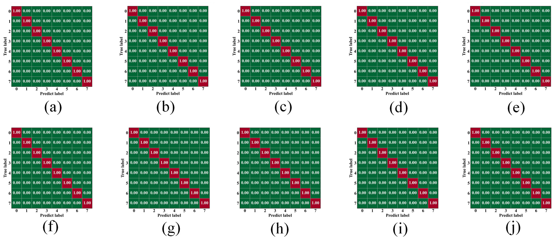
Confusion matrix after modal fusion training: (a)-(j) Confusion matrices for ten independent training runs.

In the design of the fusion network, deep integration of conductance signal features from two modalities is achieved through multilevel feature extraction and effective information fusion. Additionally, the residual connections and batch normalization modules introduced in the network architecture not only deepen the network’s hierarchical structure but also effectively alleviate the vanishing gradient problem in deep network training, ensuring training stability and efficiency. Batch normalization performs standardization processing in each network layer, reducing internal covariate shift, significantly accelerating model convergence speed, while enhancing the model’s generalization capability.

To further investigate the advantages of multilevel fusion networks and bidirectional attention fusion modules, this study installed t-SNE hooks at the pre-fusion, intermediate fusion layers, and final fusion layers, enabling effective monitoring of key node features. The following detailed analysis of t-SNE diagrams from three probe groups at different stages (as shown in Figure 17) thoroughly discusses the results of three control experiments conducted under the same method and experimental conditions, aiming to evaluate the robustness and adaptability of this method.

Figure 17.

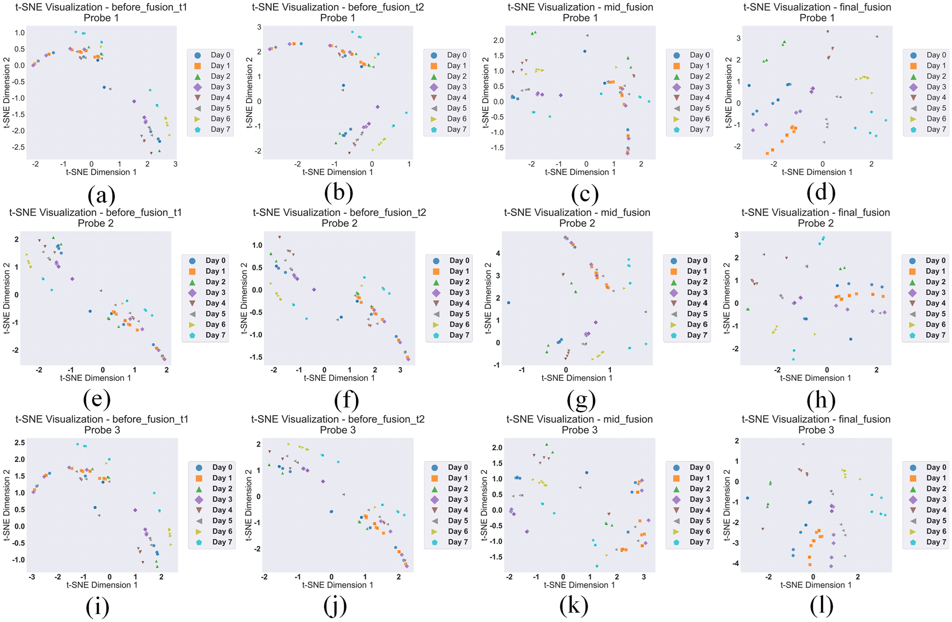
t-SNE visualization of feature distributions at different fusion stages: (a)-(d) Probe 1 features at before_fusion_t1, before_fusion_t2, mid_fusion, and final_fusion stages, and (e)-(h) Probe 2 features at corresponding stages. (i)-(l) Probe 3 features at corresponding stages.

Before_fusion_t1 as shown in Figure 17(a) and Before_fusion_t2 as shown in Figure 17(b) display different feature distribution patterns. t1 shows a distinct layered structure from top to bottom, with an overall loose distribution and unclear boundaries between classes. t2 exhibits a diagonal distribution pattern, showing stronger polarization characteristics compared to t1. In the middle fusion layer (mid_fusion) as shown in Figure 17(c), the data show a dispersed but regular distribution pattern, with Day 0 and Day 5 data points relatively concentrated, Day 2 and Day 6 data points mainly distributed in the upper region, and the remaining data points, although scattered, maintain relatively independent distribution areas. In contrast, the final fusion layer (final_fusion) demonstrates clearer temporal evolution characteristics, with data points generally showing a distribution trend from left to right and bottom to top.

Final_fusion demonstrates superior feature representation capabilities and data distribution characteristics compared to mid_fusion. From Figure 17(d), it can be observed that the data points exhibit a more regular radial distribution pattern in two-dimensional space, with data points from Day 2, Day 4, Day 6, and Day 7 (green, brown, yellow, cyan) arranged in an orderly manner, while data points from Day 0, Day 1, Day 3, and Day 5 (blue, orange, purple, gray) extend toward the lower left corner, forming a clear temporal evolution trajectory. Compared to mid_fusion, final_fusion not only maintains good interclass separation but also achieves more compact intraclass aggregation, with data points from each day being more concentrated and having clearer boundaries. Particularly in the transition areas, final_fusion shows more natural gradient characteristics, maintaining continuity between adjacent time points while effectively reflecting the feature differences between different periods. This multistage fusion strategy successfully integrates feature information from different levels, accurately capturing the dynamic evolution characteristics of the corrosion process while maintaining data separability.

The t-SNE plots of probe two and probe three reflect characteristics consistent with the previous probes, further validating the advantages of multilevel fusion strategy in feature representation. During the analysis of corrosion monitoring data, we observed a gradual enhancement in feature expression capability: from the distinct distribution characteristics of two independent modalities before fusion (modality 1 showing diagonal distribution, modality 2 showing layered structure), to the more organized structure displayed in the middle fusion layer (mid_fusion), and finally to the clear clustering structure formed in the final fusion layer (final_fusion). The entire process clearly demonstrates the progressive evolution of feature optimization, with the model’s ability to capture temporal features significantly improving as fusion levels deepen, particularly excelling in early-stage feature extraction. This hierarchical feature fusion strategy not only achieved a transformation from “chaos” to “order” while preserving the complementarity of original modalities but also accomplished optimal feature combination; through t-SNE visualization results, we can observe the gradual improvement in feature expression capability, ultimately forming high intraclass cohesion and interclass separation. This multilevel processing approach not only provides important experimental evidence for understanding the evolutionary characteristics of deep learning models in feature learning processes but also offers strong support for improving corrosion monitoring system performance, confirming the superiority of this strategy in handling complex temporal data.

To quantify the effects of multilevel fusion strategies, we introduced multiple evaluation metrics for comprehensive assessment of model performance. Dimension utilization refers to the proportion of effectively utilized feature dimensions to total feature dimensions, where higher dimension utilization indicates more features are fully utilized, enhancing the model’s expressiveness and accuracy. Category overlap ratio measures the degree of sample overlap between different categories, where higher category overlap indicates lower distinction between categories, potentially leading to increased classifier misidentification. Feature discrimination indicates the ability of features to distinguish between different categories, where higher feature discrimination means features can more effectively differentiate categories, improving classification performance. Category separation describes the degree of separation between different categories in feature space, where good category separation indicates large interclass distances without interference, contributing to improved classification accuracy. Clustering effect evaluates the ability of clustering algorithms to group similar samples together, where good clustering effect means samples within classes are tightly grouped while showing clear differences between classes. Finally, overall performance comprehensively measures the model or method’s performance across various metrics, including accuracy, stability, and robustness, reflecting the model’s comprehensive capabilities.

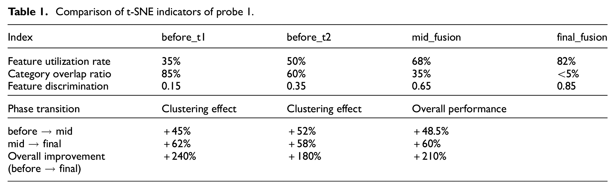
The t-SNE results of probe No. 1 are shown in Table 1. The initial phase (before_t1) data shows a dimensional utilization rate of 35%, a category overlap ratio of up to 85%, and a feature discrimination of only 0.15, indicating significant deficiencies in feature extraction and category discrimination in the unprocessed method. As the experiment progressed through multiple processing stages, the dimensional utilization rate in the final fusion stage increased to 82%, the category overlap ratio decreased to less than 5%, and the feature discrimination improved to 0.85, demonstrating the method’s efficiency in optimizing initial data. Overall, from the initial stage to the final fusion stage, category separation improved by 240%, clustering effect improved by 180%, and overall performance improved by 210%, fully proving the robustness and effectiveness of this method.

Table 1.

Comparison of t-SNE indicators of probe 1.

Index	before_t1	before_t2	mid_fusion	final_fusion
Feature utilization rate	35%	50%	68%	82%
Category overlap ratio	85%	60%	35%	<5%
Feature discrimination	0.15	0.35	0.65	0.85
Phase transition	Clustering effect	Clustering effect	Overall performance
before → mid	+45%	+52%	+48.5%
mid → final	+62%	+58%	+60%
Overall improvement(before → final)	+240%	+180%	+210%

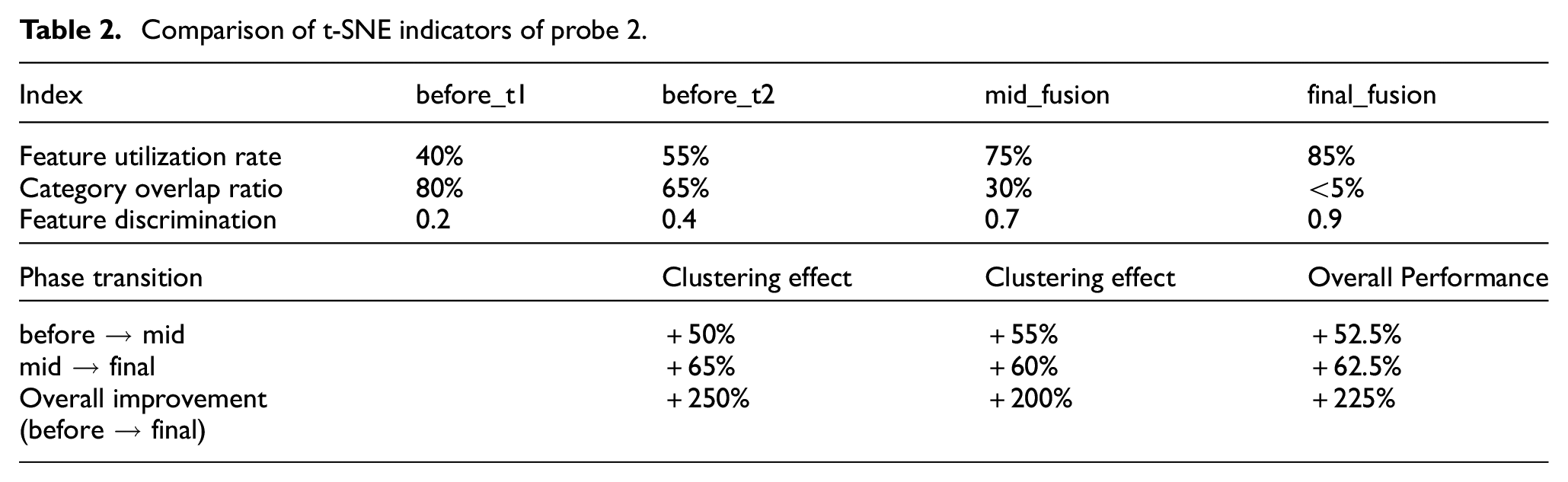
The t-SNE metrics of probe No. 2 are shown in Table 2. The initial phase (before_t1) data shows a dimensional utilization rate of 40%, a category overlap ratio of up to 80%, and a feature discrimination of only 0.2, indicating significant deficiencies in feature extraction and category discrimination in the unprocessed method. As the experiment progressed, the final fusion phase showed an increase in dimensional utilization to 85%, a decrease in category overlap to less than 5%, and an improvement in feature discrimination to 0.9, demonstrating the method’s effectiveness in optimizing initial data. Overall, from the initial phase to the final fusion phase, category separation improved by 250%, clustering effectiveness increased by 200%, and overall performance improved by 225%, further validating the significant role of this method in enhancing system performance and accuracy.

Table 2.

Comparison of t-SNE indicators of probe 2.

Index	before_t1	before_t2	mid_fusion	final_fusion
Feature utilization rate	40%	55%	75%	85%
Category overlap ratio	80%	65%	30%	<5%
Feature discrimination	0.2	0.4	0.7	0.9
Phase transition		Clustering effect	Clustering effect	Overall Performance
before → mid		+50%	+55%	+52.5%
mid → final		+65%	+60%	+62.5%
Overall improvement(before → final)		+250%	+200%	+225%

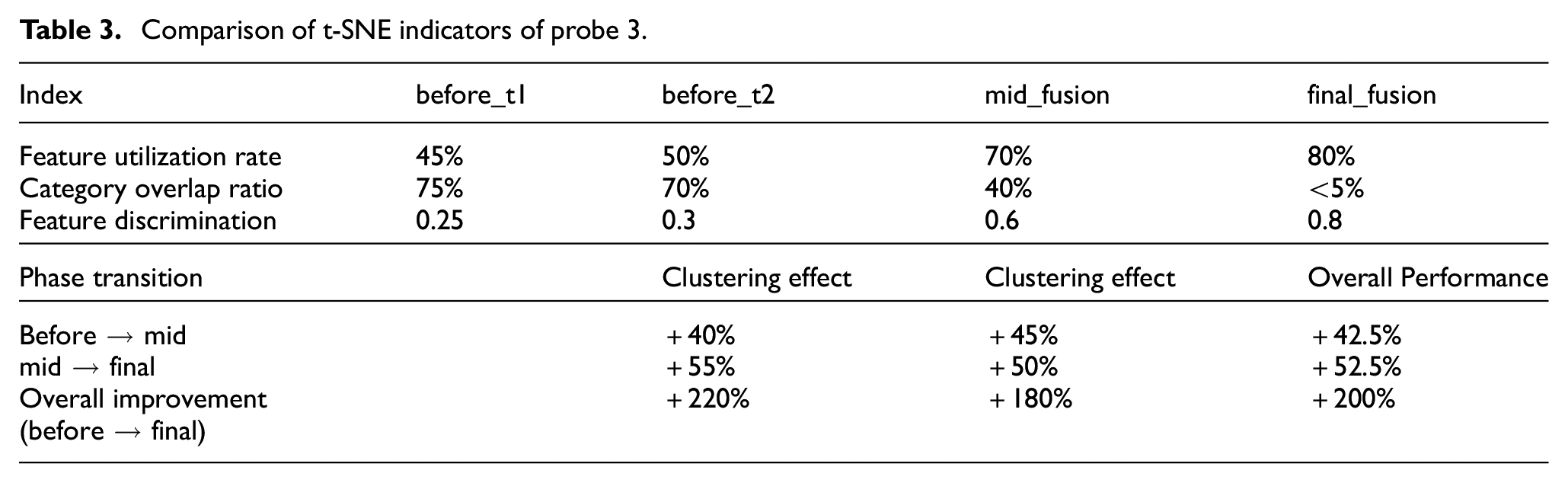
The t-SNE metrics of probe 3 are shown in Table 3. In the initial phase (before_t1), the data shows a dimensional utilization rate of 45%, a category overlap ratio of 75%, and a feature discrimination of only 0.25, indicating significant deficiencies in feature extraction and category discrimination in the unprocessed method. During the intermediate fusion stage (mid_fusion), the dimensional utilization rate increased to 70%, the category overlap ratio decreased to 40%, and the feature discrimination improved to 0.6, demonstrating the crucial role of multistage fusion in optimizing features and reducing category overlap. In the final fusion stage (final_fusion), the dimensional utilization rate further increased to 80%, the category overlap ratio decreased to less than 5%, and the feature discrimination improved to 0.8, proving the significant importance of multistage fusion for continuous system performance improvement. Overall, from the initial stage to the final fusion stage, category separation improved by 220%, clustering effect improved by 180%, and overall performance improved by 200%, demonstrating the effectiveness of multistage fusion in improving system efficiency and accuracy.

Table 3.

Comparison of t-SNE indicators of probe 3.

Index	before_t1	before_t2	mid_fusion	final_fusion
Feature utilization rate	45%	50%	70%	80%
Category overlap ratio	75%	70%	40%	<5%
Feature discrimination	0.25	0.3	0.6	0.8
Phase transition		Clustering effect	Clustering effect	Overall Performance
Before → mid		+40%	+45%	+42.5%
mid → final		+55%	+50%	+52.5%
Overall improvement(before → final)		+220%	+180%	+200%

The results of three sets of control experiments show that despite minor fluctuations between different experiments, the overall trends and key indicators remain highly consistent, demonstrating the stability and reliability of the proposed method across multiple independent experiments. The steady improvement in dimensional utilization, effective reduction in category overlap ratio, and continuous enhancement in feature discrimination all indicate that this method has significant effects in enhancing data feature representation and category discrimination capabilities. However, the category overlap ratio remains relatively high, indicating that in complex datasets, the method still has room for improvement in completely eliminating intercategory overlap, requiring further optimization in the future to enhance overall performance.

Comparative test results analysis

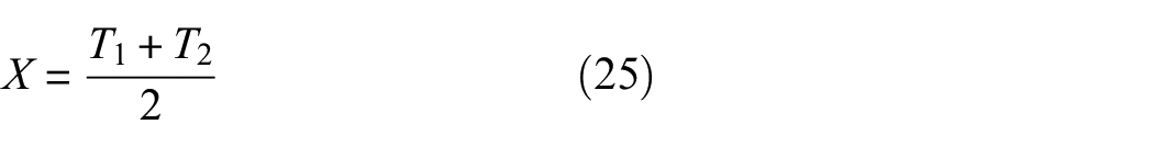
This study comparatively analyzes three common basic fusion network methods—Early Fusion, Late Fusion, and Average Fusion, and compares their performance with the proposed BMFN network. To comprehensively evaluate the robustness and adaptability of each method, these methods were tested under different signal-to-noise ratio (SNR) conditions with simultaneous noise addition to axial vibration mode and bending vibration mode, as shown in Figure 18. These basic fusion methods each have their characteristics: Early fusion integrates data from different sources at the feature level, which can fully utilize the complementary information of multisource data to enhance the model’s expressiveness, but may face issues of feature alignment and dimensional inconsistency. Late fusion integrates data from different sources at the decision level, where modal data are processed through independent models before weighted averaging or voting fusion, offering advantages in flexibility and modular design, but may fail to fully capture potential intermodal correlations. Average fusion, as a simple late fusion strategy, obtains final predictions by averaging the output results of independent models, and while simple to implement with low computational cost, it performs poorly when handling cases with significant performance differences between models, as it cannot adaptively allocate weights to different models, limiting overall performance.

Figure 18.

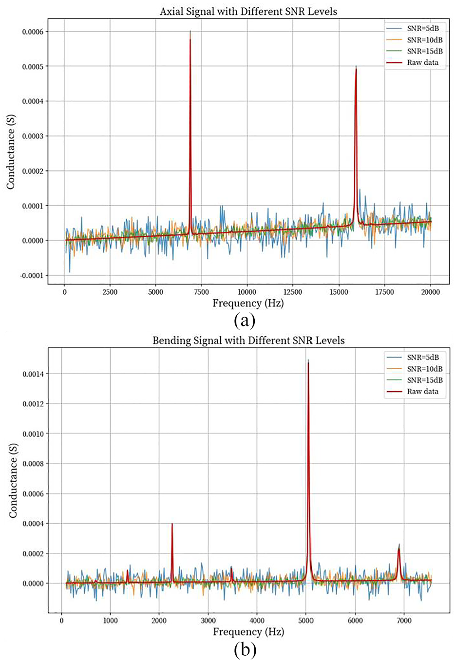
(a) Axial mode conductance curves at different SNR and (b) bending mode conductance curves at different SNR.

The experimental results are shown in Figure 19. Under all signal-to-noise ratio conditions, the BMFN network achieves higher accuracy than other fusion methods, particularly in low SNR (5 dB) conditions, where the BMFN network’s accuracy is approximately 10 percentage points higher than late fusion, demonstrating stronger robustness and adaptability in environments with significant noise interference. As SNR increases, the accuracy of various fusion methods generally improves, indicating that signal quality enhancement has a significant positive impact on model performance. Under high SNR (15 dB) conditions, early fusion, late fusion, and BMFN network all achieve 100% accuracy, showing that these methods can achieve perfect classification under favorable signal conditions. Specifically, early fusion performs excellently under high SNR conditions but relatively weakly under low SNR, possibly due to noise accumulation at the feature level affecting the model’s discriminative ability; late fusion outperforms early fusion and average fusion under all SNR conditions, particularly under medium SNR (10 dB) conditions, where its accuracy approaches that of the BMFN network, demonstrating good balance; average fusion, as the simplest fusion strategy, performs the weakest under all conditions, mainly because it cannot effectively integrate the advantages of different models, limiting overall performance.

Figure 19.

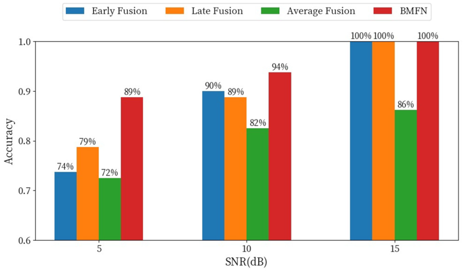
Performance of different fusion methods under noisy conditions.

The experimental results further demonstrate that the fused features exhibit enhanced robustness, maintaining high classification performance even in the presence of noise interference. This is primarily attributed to multimodal fusion’s ability to integrate redundant information from different time periods, effectively counteracting noise effects in individual signals and improving the overall system’s stability and reliability.

Discussion and conclusion

In response to the insufficient multimodal information fusion in current conductance signal processing and corrosion state diagnosis, which makes it difficult to comprehensively and accurately assess equipment corrosion conditions, this study proposes a corrosion monitoring method based on multimodal fusion neural network. The main contributions include

A new multimodal fusion framework of the resonance characteristics of the two modes was proposed, which organically combines the signal characteristics of the axial mode and the bending mode. The axial mode is outstanding in the clarity of the double-peak characteristics, and the bending mode provides richer modal information. The frequency responses of the two complement each other, providing a reliable basis for the comprehensive evaluation of material properties. The experimental results show that within their respective characteristic frequency ranges, both modes exhibit excellent signal stability and data repeatability, laying a solid foundation for subsequent damage monitoring and life assessment.

The logarithmic frequency dual attention module was proposed, which innovatively introduces first-order derivative attention and second-order derivative attention to enhance the feature extraction capability. First-order derivative attention emphasizes the instantaneous change of the signal and is suitable for capturing rapidly changing features; second-order derivative attention focuses on the curvature change of the signal and is suitable for capturing complex dynamic features. Fusion attention combines the advantages of the two derivative attentions, achieves more comprehensive and flexible feature extraction, improves the accuracy and stability of the model, and verifies its effectiveness in enhancing feature expression.

The bidirectional-attention multistage fusion network was constructed, and an advanced fusion strategy was adopted to effectively integrate multisource information at the feature level and decision level. The performance advantages of the network were verified through a comprehensive analysis of three sets of experimental results. First, the method has good repeatability, and the trends of the three sets of experimental results are consistent; second, the classification effect gradually improves as the experiment progresses, especially in probe C, reaching the best level; finally, t-SNE visualization analysis intuitively demonstrates the effectiveness of the method in feature extraction and category distinction. In particular, under low signal-to-noise ratio (SNR) conditions, the classification performance is significantly improved, which proves the effectiveness of the method in dealing with noise interference and complex signal environments.

The bidirectional-attention fusion module was proposed, which innovatively combines temporal and channel attention and adopts an additive fusion strategy to effectively capture complex spatiotemporal dependencies. The attention weights generated by the two branches are applied to the original features through additive fusion, which not only captures long-term dependencies but also provides richer feature representations while maintaining numerical stability. Compared with the traditional multiplicative attention mechanism, additive fusion can better avoid the gradient vanishing problem and improve the training stability of the model. Ablation experiments further prove the effectiveness of each key component, among which the additive fusion strategy and dual-input feature design contribute the most to performance improvement.

In summary, the corrosion quantitative monitoring method proposed in this study, based on dual-modal EMI and a bidirectional multilevel fusion network, offers significant improvements in the accuracy and robustness of conductance signal processing and corrosion state diagnosis. This approach provides an effective solution for monitoring equipment corrosion in complex industrial environments.

Although this study has achieved some meaningful results, it also has some shortcomings. Future work will focus on extending the application scope of the proposed fusion network. We plan to expand our testing environments beyond the standard 3.5% NaCl solution to include various corrosive media such as acidic and high-temperature environments, which will help validate LFDM’s adaptability across different corrosion scenarios. Additionally, extended monitoring experiments over several months to years in real-world environments will be conducted to thoroughly evaluate the method’s long-term durability and reliability. To enhance model interpretability, we will incorporate explainable AI techniques such as SHAP values and LIME to analyze the contribution of different frequency components, particularly the resonance peaks, to the network’s decisions. This analysis will provide valuable insights into why certain frequencies play more dominant roles in damage classification. Furthermore, comprehensive comparisons with advanced deep learning architectures, such as transformer-based models (which excel at capturing long-range dependencies in frequency sequences) and graph neural networks (which could potentially model the intrinsic relationships between different resonance modes), will be conducted to provide a more thorough evaluation of LFDM’s performance. To ensure practical applicability, we will evaluate the model’s real-time performance on embedded devices commonly used in industrial monitoring systems, including latency testing and necessary optimizations for efficient deployment. Specifically, classical EMI damage detection experiments with artificial defects, such as cracks and holes of different damage levels on metal plates, will be conducted to further validate the network’s performance and generalization capability. These controlled experiments will help establish the broader applicability of our fusion approach in various structural health monitoring scenarios beyond corrosion detection.

Footnotes

Author contributions

Jingyi Wei: Conceptualization, Data curation, Writing – original draft.

Jianchao Wu: Funding acquisition, Supervision.

Lei Zhu: Formal analysis, Writing – review.

Yixuan Chen: Funding acquisition, Writing – review & editing.

Wenhan Liao: Software, Validation.

Yabin Liang: Investigation, Resources.

Declaration of conflicting interests

The author(s) declared no potential conflicts of interest with respect to the research, authorship, and/or publication of this article.

Funding

The author(s) disclosed receipt of the following financial support for the research, authorship, and/or publication of this article: The research reported in this study was partially supported by Hubei Provincial Natural Science Foundation of China (2023AFB859), the Postgraduate Research & Practice Innovation Program of Jiangsu Province (No. SJCX24_0085), the SEU Innovation Capability Enhancement Plan for Doctoral Students (No. CXJH_SEU 24096).

ORCID iDs

Jianchao Wu

Yixuan Chen

References

Revie

Uhlig

. Corrosion and corrosion control: an introduction to corrosion science and engineering. Hoboken, NJ: John Wiley & Sons, 2008.

Mahmoodian

. Reliability and maintainability of in-service pipelines. Boston, MA: Gulf Professional Publishing, 2018.

Vasagar

Hassan

Abdullah

, et al. Non-destructive techniques for corrosion detection: a review. Corr Eng Sci Technol 2024; 59(1): 56–85.

Usarek

Warnke

. Inspection of gas pipelines using magnetic flux leakage technology. Adv Mater Sci 2017; 17(3): 37–45.

Zou

Cegla

. High accuracy ultrasonic corrosion monitoring. In: NACE corrosion, 2017, pp. NACE-2017. New Orleans, LA: NACE.

García-Martín

Gómez-Gil

Vázquez-Sánchez

. Non-destructive techniques based on eddy current testing. Sensors 2011; 11(3): 2525–2565.

Majumder

Gangopadhyay

Chakraborty

, et al. Fibre Bragg gratings in structural health monitoring—present status and applications. Sens Actuators A 2008; 147(1): 150–164.

Powell

. Internal corrosion monitoring using coupons and Er probes a practical focus on the most commonly used, cost-effective monitoring techniques. Oil Gas Pipelines 2015: 495–514.

Annamdas

VGM

Soh

. Application of electromechanical impedance technique for engineering structures: review and future issues. J Intell Mater Syst Struct 2010; 21(1): 41–59.

10.

Talakokula

Bhalla

Gupta

. Monitoring early hydration of reinforced concrete structures using structural parameters identified by piezo sensors via electromechanical impedance technique. Mech Syst Signal Process 2018; 99: 129–141.

11.

Talakokula

Bhalla

Ball

, et al. Diagnosis of carbonation induced corrosion initiation and progression in reinforced concrete structures using piezo-impedance transducers. Sens Actuators A 2016; 242: 79–91.

12.

Yang

Zhu

, et al. Experimental study on monitoring steel beam local corrosion based on EMI technique. Appl Mech Mater 2013; 273: 623–627.

13.

Han

Zhang

Wang

, et al. Structural health monitoring of timber using electromechanical impedance (EMI) technique. Adv Civil Eng 2020; 2020(1): 1906289.

14.

Park

. A cost-effective impedance-based structural health monitoring technique for steel structures by monitoring multiple areas. J Intell Mater Syst Struct 2017; 28(2): 154–162.

15.

Wang

Luo

, et al. Modeling and experimental validation of a quantitative bar-type corrosion measuring probe using piezoelectric stack and electromechanical impedance technique. Measurement 2022; 188: 110546.

16.

Liu

Wang

, et al. EMI instrumented conical corrosion measuring probe for pipeline corrosion monitoring: experiments with FEM validation. Sens Actuators A 2023; 362: 114678.

17.

Raju

Bhalla

Visalakshi

. Pipeline corrosion assessment using piezo-sensors in reusable non-bonded configuration. NDT E Int 2020; 111: 102220.

18.

Liu

Wang

Chen

, et al. Concrete damage diagnosis using electromechanical impedance technique. Constr Build Mater 2017; 136: 450–455.

19.

Zhang

Chen

, et al. Electromechanical impedance response of a cracked Timoshenko beam. Sensors 2011; 11(7): 7285–7301.

20.

De Oliveira

Monteiro

Vieira Filho

. A new structural health monitoring strategy based on PZT sensors and convolutional neural network. Sensors 2018; 18(9): 2955.

21.

Chen

Jiang

Qin

, et al. Quantitative monitoring of bolt looseness using multichannel piezoelectric active sensing and CBAM-based convolutional neural network. Front Mater 2021; 8: 677642.

22.

Zhu

, et al. Integrated electromechanical impedance technique with convolutional neural network for concrete structural damage quantification under varied temperatures. Mech Syst Signal Process 2021; 152: 107467.

23.

Yan

Liao

Zhang

, et al. Intelligent monitoring and assessment on early-age hydration and setting of cement mortar through an EMI-integrated neural network. Measurement 2022; 203: 111984.

24.

Han

, et al. Automated identification of compressive stress and damage in concrete specimen using convolutional neural network learned electromechanical admittance. Eng Struct 2022; 259: 114176.

25.

Cheng

, et al. Deep learning of electromechanical impedance for concrete structural damage identification using 1-D convolutional neural networks. Constr Build Mater 2023; 385: 131423.

26.

Yang

Gao

Chen

, et al. A novel electromechanical impedance-based method for non-destructive evaluation of concrete fiber content. Constr Build Mater 2022; 351: 128972.

27.

Cheng

. A deep learning approach for electromechanical impedance based concrete structural damage quantification using two-dimensional convolutional neural network. Mech Syst Signal Process 2023; 183: 109634.

28.

Alexander

Sumathi

Panigrahi

, et al. Embedded dual PZT-based monitoring for curing of concrete. Constr Build Mater 2021; 312: 125316.

29.

Shen

Sun

. Squeeze-and-excitation networks. In: Proceedings of the IEEE conference on computer vision and pattern recognition, Salt Lake, UT, 2018, pp. 7132–7141.

30.

Woo

Park

Lee

, et al. CBAM: convolutional block attention module. In: Proceedings of the European conference on computer vision (ECCV), Munich, Germany, 2018, pp. 3–19.

31.

Hou

Zhou

Feng

. Coordinate attention for efficient mobile network design. In: Proceedings of the IEEE/CVF conference on computer vision and pattern recognition, Virtual, 2021, pp. 13713–13722.