Digital twin-driven feature enhancement generative adversarial network for rolling bearings fault diagnosis

Abstract

The difficulty of collecting fault samples of bearings under stable operation results in imbalanced data and considerably weakened capability of the deep learning-based intelligent fault diagnosis methods. Thus, a novel digital twin (DT)-driven feature enhancement generative adversarial network (DFGAN) was proposed in this study to augment the imbalanced multisensor data and improve diagnostic accuracy. First, a generic DT model with multiple degrees of freedom was developed to obtain simulated vibration data containing fault features. Subsequently, DFGAN was adopted to translate simulated data into measured data and generate synthetic samples with distributions similar to those of the measured samples. Specifically, the DFGAN incorporated an improved squeeze-and-excitation U-Net as the generator and integrated a spectral correlation loss to enhance the quality of synthetic samples. Finally, the imbalanced multisensor data were augmented with the synthetic samples, and bearing fault diagnosis was achieved by a multibranch convolutional neural network. Furthermore, the proposed method was verified to diagnose two rolling bearing datasets. The results reveal that the proposed method effectively augmented imbalanced data and significantly enhanced diagnostic performance.

Keywords

Imbalanced data data augmentation digital twin generative adversarial network rolling bearing

Introduction

Rotating machinery plays an important role in the fields of energy conversion, power transmission, and automation control. With advancements in industrial development, rotating machinery is evolving toward highly intelligent integration and enhanced reliability. As a critical component of rotating machinery, rolling bearings may fail under extreme operating conditions, resulting in the loss of human life and impacting industrial manufacturing.^1,2 Therefore, real-time monitoring and diagnosis of bearing operating conditions is critical for ensuring safe operation and reducing system maintenance costs.

Data-driven deep learning (DL) methods have demonstrated high performance in bearing fault diagnosis in the last decade. Classical models, such as long short-term memory (LSTM),³ denoising autoencoder,⁴ convolutional neural network (CNN),⁵ deep belief network,⁶ along with their variants,^7–9 have achieved high diagnostic accuracy and widespread application. Data-driven methods can still be applicable to challenging diagnostic tasks. Liang et al.¹⁰ integrated Stockwell transform and data augmentation method with a capsule neural network (CapsNet) to diagnostic the compound fault of wind turbine gearboxes. Zhang et al.¹¹ proposed a novel self-supervised graph neural network, which utilizes negative-sample-free contrastive learning and scale attention mechanism to solve the problems of underutilization of graph features in fault diagnosis. Li et al.¹² proposed a method that converts raw vibration signals into envelope spectra through combined Hilbert and Fourier transforms. They designed architecture combined CNN and CapsNet, which effectively maintains spatial features, achieving superior diagnostic accuracy. Xu et al.¹³ used cascadic multireceptive learning network to construct a feature extractor for obtaining rich multilevel features from monitoring signals, which improves the performance of the diagnostic model. Zhong et al.¹⁴ designed a two-branch GCN combined with an improved bidirectional gated recurrent unit to integrate spatial and temporal features of feature samples. The extracted domain-invariant features are utilized to achieve cross-domain fault diagnosis of bearing. Some studies have fused multisensor features to overcome the limitations of single-sensor data and improve fault diagnosis accuracy. For example, Zhang et al.¹⁵ introduced structural attention into multiscale group Mamba network to efficiently extract fault features from multisensor data of rotating machinery for diagnostic tasks. Yan et al.¹⁶ designed a multibranch convolutional neural network (MCNN) and implemented an end-to-end multisensor data fusion mechanism for fault diagnosis of rotating machinery. In addition, Wang et al.¹⁷ extracted and fused features from vibration and sound signals using a CNN, achieving fault diagnosis of rolling bearings. Furthermore, Ma et al.¹⁸ designed a dual-branch CNN with a multiscale attention module to achieve multisensor information fusion and equipment fault diagnosis. Using information entropy to calculate fusion weights, Zhang et al.¹⁹ proposed a dual-level data fusion model for bearing fault diagnosis, incorporating a multimodal image fusion strategy. However, data-driven DL methods require sufficient fault samples to achieve effective fault feature extraction.²⁰ In applications, it is challenging to collect fault samples during the safe operation of a system, leading to imbalanced data and greatly reducing the capability of most DL-based models.²¹

Generative adversarial networks (GANs) can be used to learn the feature distribution of fault data and transform random noise into a distribution similar to that of real data through learning mapping, making them an effective method for imbalanced bearing fault diagnosis.^21–23 Liang et al.²⁴ transformed vibration signals into time–frequency images and augmented an imbalanced dataset using a GAN. Pan et al.²⁵ incorporated a feature extractor into a conditional GAN to acquire the feature distribution of real data, allowing networks to output rich synthetic fault features by introducing additional sequences. To stabilize the training process, many researchers have employed Wasserstein GANs (WGANs), which utilize the Wasserstein distance as the loss function of the discriminator instead of the Jensen–Shannon divergence.²⁶ Li et al.²⁷ introduced a strategy based on an auxiliary classifier GAN, which employs the Wasserstein distance and spectral normalization to optimize the loss function of the discriminator. Su et al.²⁸ encoded fault samples using a kurtosis perceptron, feeding the encoded features into a WGAN to generate synthetic samples for imbalanced data. Gu et al.²⁹ incorporated cosine similarity loss into WGAN with gradient penalty (WGAN-GP), improving the stability of synthetic sample generation and the diagnostic accuracy. Guo et al.³⁰ improved the generator structure of WGAN-GP using convolutional variational autoencoding to improve the effectiveness of output samples. Li et al.³¹ introduced domain classifier into WGAN-GP to generate pseudo samples, achieving cross-domain fault diagnosis for imbalanced samples. Although GANs and their variants address the limitations of imbalanced data, their training process is highly unstable.³² In the absence of fault samples, the synthetic samples generated by GANs are ineffective and provide limited improvement in imbalanced fault diagnosis.

Digital twin (DT) technology is an innovative approach to addressing the aforementioned challenges,^33,34 with simulated signals obtained from DT models improving diagnostic accuracy.^35,36 In the past year, several transfer learning (TL) frameworks for imbalanced fault diagnosis utilizing DT models have been proposed. Li et al.³⁷ improved CNN model by employing focus modulation to learn the features of simulated samples generated by the DT model, enhancing the diagnosis performance. To address insufficient fault data, Yan et al.³⁸ obtained simulated signals generated by a finite-element-based DT model, which trained the TL network with a subdomain adaptive mechanism for imbalanced fault diagnosis. In addition, Zhang et al.³⁹ developed a high-fidelity DT model for rolling bearings and designed a TL framework with an adversarial strategy to learn fault features in simulated data for diagnosis.

Combining DT technology with GANs provides new opportunities to fully utilize the fault information contained in simulated data, thus improving fault diagnosis performance.⁴⁰ Xia et al.⁴¹ constructed a DT model of a gear system to generate simulated vibration signals and fused simulated and measured data using a WGAN. The fused samples improved diagnostic accuracy under imbalanced data conditions. Using a cycle-consistent GAN (CycleGAN), Liu et al.⁴² extended simulated bearing fault data for fault diagnosis. Qin et al.⁴³ improved CycleGAN using LSTM to establish a mapping between measured and simulated signals from the DT model, enabling imbalanced data augmentation.

The combination of GANs and DT is advantageous in that simulated data generated by the DT model contain a large amount of fault information, facilitating stable GAN training. In addition, GANs help bridge the gap between simulated and measured signals, greatly enhancing the auxiliary effect of simulated signals in imbalanced bearing fault diagnosis. However, diverse service conditions make it difficult to construct a generic DT model with high simulation accuracy, and the synthetic data generated by GANs may differ from the measured data, particularly in the frequency domain. These factors limit the effectiveness of DT technology.⁴⁴

Therefore, the main problems of existing data augmentation methods that combine DT and GAN are detailed as follows: (1) The traditional DT modeling method ignores the internal force state of the bearing, leading to lower generality and simulation accuracy. (2) Existing GAN models cannot adequately retain the simulated fault information of the DT model when synthesizing samples. (3) The frequency domain distributions of the synthetic samples differ from those of the measured samples in the absence of explicit constraints on their frequency-domain features. To address the above issues, this article introduces a novel method for imbalanced fault diagnosis of rolling bearings. This method combines a generic high-fidelity DT model and a DT-driven feature enhancement generative adversarial network (DFGAN) to generate synthetic samples. Unlike the existing methods, the degrees of freedom (DOFs) of each bearing component are innovatively considered in the DT model to reinforce generalizability and simulation accuracy. Additionally, an improved generator named squeeze-and-excitation U-Net (SEU-Net) is utilized in DFGAN to adaptively select effective simulated fault information from the DT model to be fused into the synthetic samples. Moreover, the loss function of DFGAN is improved to constrain the frequency distribution of the synthetic samples based on the correlation of spectrums. An overview of the proposed method is given in Figure 1. First, a generic high-fidelity DT model with multiple DOFs is developed to simulate the bearing fault state and acquire the simulated dynamic response of the system. Subsequently, a DFGAN is introduced with the purpose of learning the mapping between measured and simulated data and generate synthetic samples of the measured samples. Finally, imbalanced multisensor data are augmented with synthetic samples to improve fault diagnosis accuracy. The main contributions of this study are summarized as follows:

A generic high-fidelity DT model of rolling bearings with multiple DOFs is developed using the lumped parameter method, employing fault and structure parameters as inputs. By considering the translational and rotational DOFs of the rollers, inner race, and outer race, the proposed DT model generates simulated vibration data containing sufficient fault feature information, thereby aiding in the diagnosis of bearing faults.

DFGAN is proposed to bridge the gap between simulated and measured samples and generate synthetic samples with a data distribution similar to that of measured signals. An improved generator called SEU-Net is designed to perform multilayer deep fusion of fault information from the simulated samples. In addition, a spectral correlation loss function (L_F) is designed to minimize the discrepancy between the frequency components of synthetic and measured samples.

The synthetic fault samples generated by DFGAN are utilized to augment imbalanced multisensor data. Then, multisensor data fusion is achieved using MCNN, improving bearing imbalanced fault diagnosis accuracy.

Figure 1.

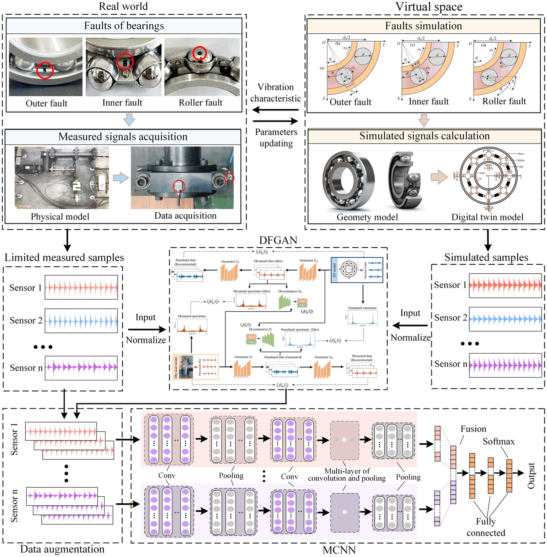
Overview of the proposed framework.

The DT model of bearings

Localized defects on the surface of rolling bearings lead to abnormal contact between the rollers and raceways, thereby exciting excitations of time-varying displacement in the system. Developing a DT model of rolling bearings to simulate localized bearing faults and obtain simulated vibration signals containing fault features is critical for fault diagnosis. The dynamic response of rolling bearings obtained from the DT model should accurately reflect the features of the measured signals of the system in both the time and frequency domains. The information interaction between the DT and physical models is illustrated in Figure 2.

Figure 2.

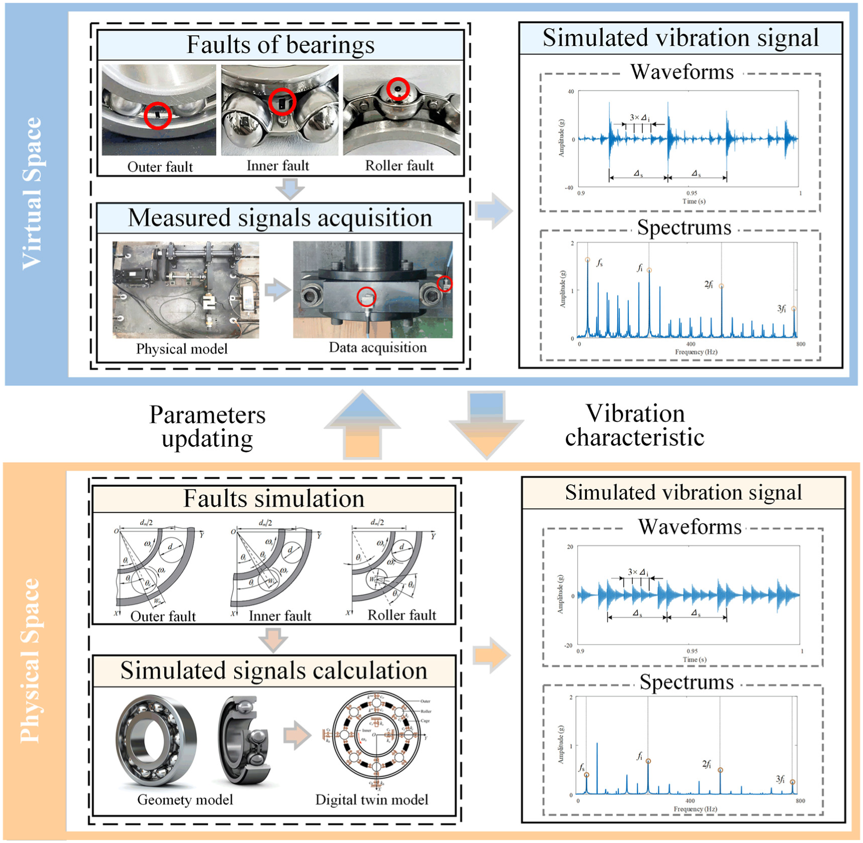
Information interaction between DT model and physical model.

Development of DT model

Ignoring the force states of the internal parts of the bearings, existing DT models rely heavily on the DOF of the inner and outer raceways to solve the simulated fault signals. In this section, thus, a generic high-fidelity DT model is developed to simulate the fault states of a rolling bearing. Different from the existing bearing DT modeling method, the high-fidelity DT model proposed in this article fully considers the motion of each part in the bearing. Except for the inner and outer raceways, the rollers and cage are also analyzed regarding force. Meanwhile, the DOFs of each part are considered in the proposed DT model to improve the simulation accuracy. As shown in Figure 3, the DT model consists of a total of 4 + 3(N_b + 1) DOFs, where N_b represents the number of rollers. In the model, the stiffness of the shaft and housing shell is represented by k_s and k_h, respectively, while the corresponding damping is represented by c_s and c_h. The contact stiffness between the rollers and raceways is denoted by k_in and k_out, with the corresponding damping denoted by c_i and c_o. In addition, the contact stiffness between the roller and cage is represented by k_j, with the damping represented by c_j. These parameters are described in detail in Liu and Shao.⁴⁵

Figure 3.

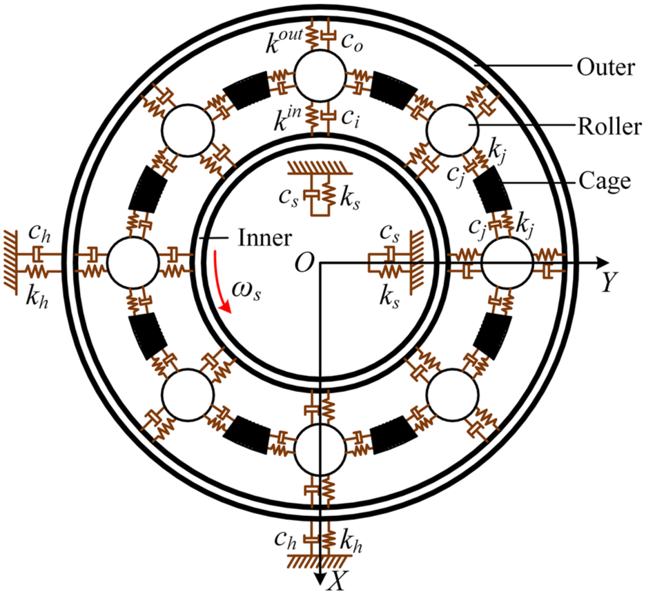
DT model of a rolling bearing.

As illustrated in Figure 4(a), when the bearing is operating stably, there is a complex interaction between its components. Under the action of radial load, the roller experiences contact and friction forces with the inner and outer raceways. The relationship between the rolling bearing load and contact deformation is as follows:

[\begin{matrix} F_{k j}^{in} \\ F_{k j}^{out} \\ F_{c j} \end{matrix}] = [\begin{matrix} k_{in} {(δ_{j}^{in})}^{n} \\ k_{out} {(δ_{j}^{out})}^{n} \\ k_{j} δ_{c j} + c_{j} {\overset{\cdot}{δ}}_{c j} \end{matrix}]

(1)

[\begin{matrix} f_{k j}^{in} \\ f_{k j}^{out} \\ f_{c j} \end{matrix}] = [\begin{matrix} μ_{b} F_{k j}^{in} \\ μ_{b} F_{k j}^{out} \\ μ_{c} F_{c j} \end{matrix}]

(2)

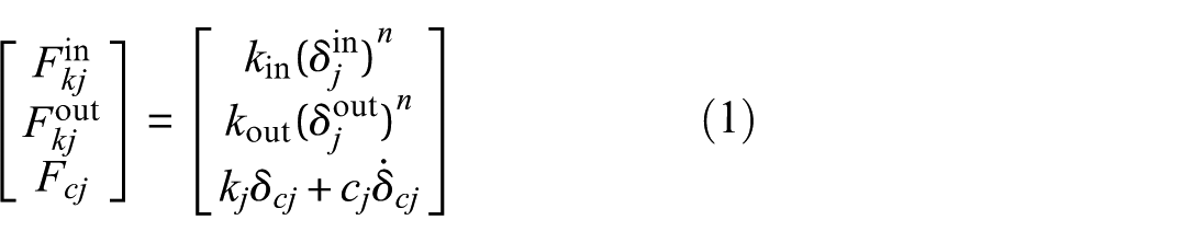
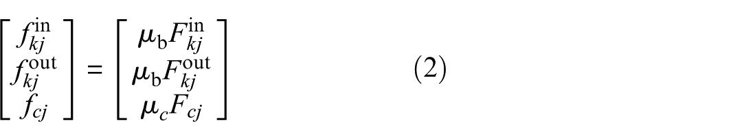
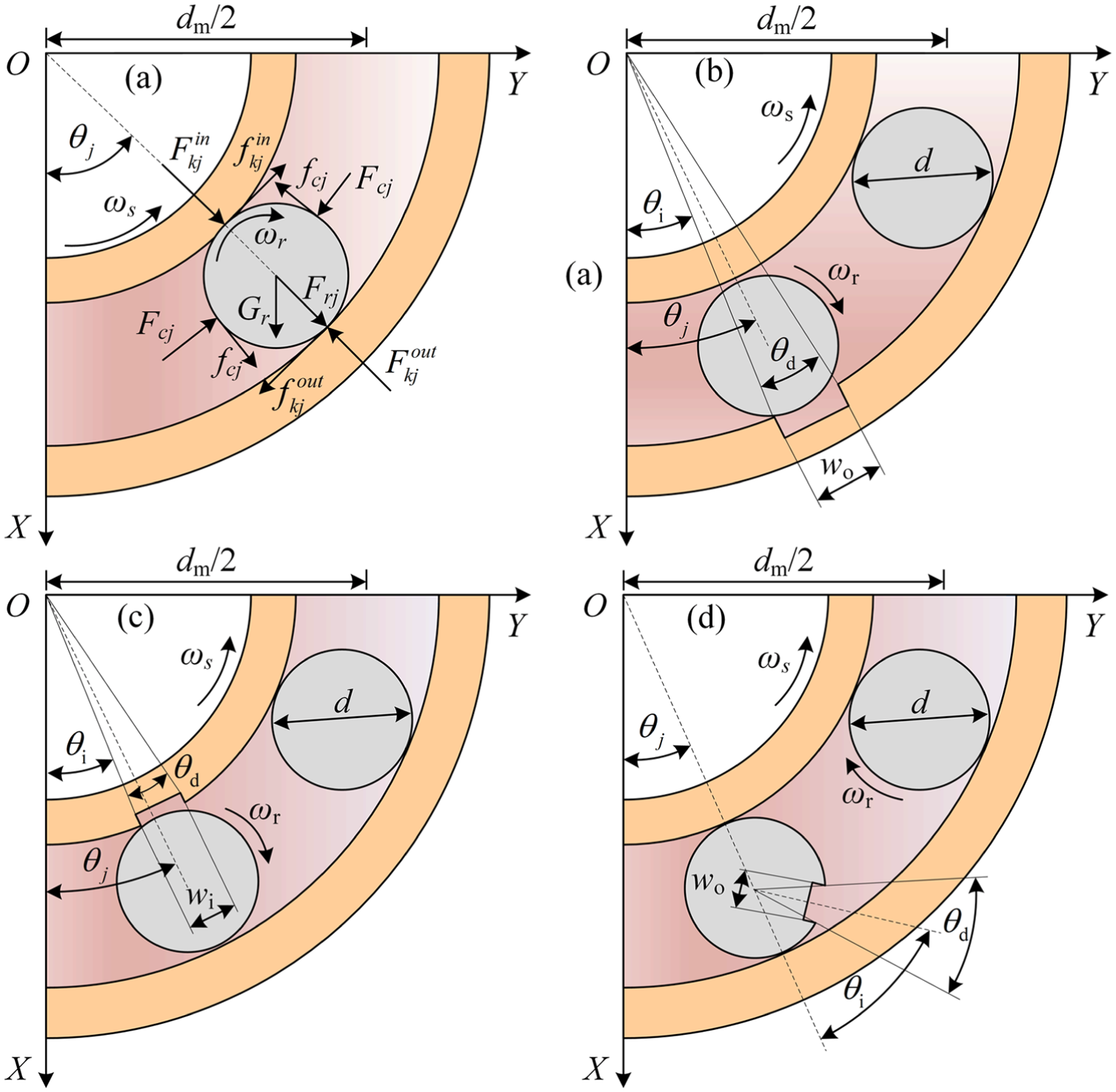
where n = 3/2 for rolling bearings, μ_b is the coefficient of friction between the roller and raceway, and μ_c is the coefficient of friction between the roller and cage. The calculation of μ_b and μ_c is provided in Gupta.⁴⁶ In addition, $δ_{j}^{in}$ and $δ_{j}^{out}$ denote the contact deformation of the j-th roller with the inner and outer races, respectively, resulting in the contact forces $F_{k j}^{in}$ and $F_{k j}^{out}$ . Furthermore, δ_jⁱⁿ denotes the contact deformation between the roller and cage, with the corresponding contact force denoted by F_cj. The damping coefficient is represented by c_j.⁴⁷ The friction forces $f_{k j}^{in}$ , $f_{k j}^{out}$ , and f_cj are generated by $F_{k j}^{in}$ , $F_{k j}^{out}$ , and F_cj, respectively.

Figure 4.

Structure of spalling faults: (a) healthy, (b) outer race faults, (c) inner race faults, and (d) roller faults.

Under a given operating condition, the load brings about a compressive deformation between the rollers and raceways of the bearing. This forms an elliptical contact surface, presenting a typical Hertz contact. The contact state is related to the structure and load of the bearing. At this time, the contact stiffness between the rollers and raceways serves as the Hertz contact stiffness, which can be expressed as follows:

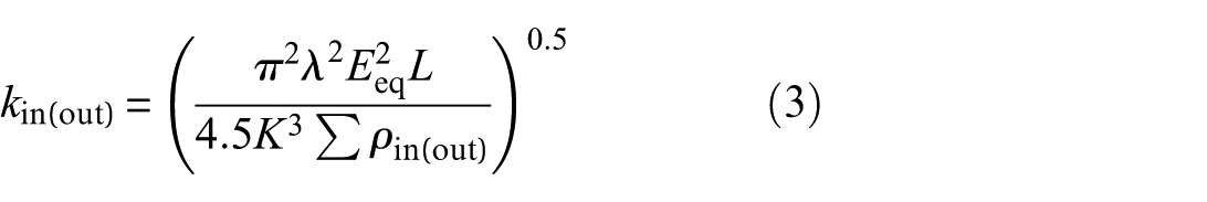
k_{in (out)} = {(\frac{π^{2} λ^{2} E_{eq}^{2} L}{4.5 K^{3} \sum ρ_{in (out)}})}^{0.5}

(3)

where E_eq is the equivalent Young’s modulus of the material in the two contacting objects, λ is the parameter of the point contact elliptic eccentricity. K and L are elliptic integrals of the first and second kind, respectively. $\sum ρ_{in}$ and $\sum ρ_{out}$ denote the curvature sum of the roller in contact with the inner and outer raceway, respectively. The calculation of the above parameters is detailed in Liu and Shao.⁴⁵

The damping of bearing is usually set in the range of 0.25 × 10⁻⁵–2.5 × 10⁻⁵ times the bearing stiffness.⁴⁸ Therefore, the damping c_i and c_o in the Hertz contact zone between the rollers and the raceways can be obtained from the following formula:

c_{i (o)} = (0.25 - 2.5) \times 10^{- 5} k_{in (out)}

(4)

When a bearing has a localized defect, rollers enter and exit the defective region with a fixed period. This defect increases the displacement range of the rollers, causing time-varying displacement of the system. Figure 4(b) to (d) illustrates the localized fault structures of the outer race, inner race, and roller, respectively. The time-varying displacement can be described using a half-sine function, as follows:

H_{do} = {\begin{matrix} H_{o max} \sin (π / θ_{d} (mod (θ_{j}, 2 π) - θ_{i})), & - θ_{d} / 2 \leq mod (θ_{j}, 2 π) - θ_{i} \leq θ_{d} / 2 \\ 0, & other \end{matrix}

(5)

H_{di} = {\begin{matrix} H_{imax} \sin (π / θ_{d} (mod (θ_{j} - ω_{s} t, 2 π) - θ_{i})), & - θ_{d} / 2 \leq mod (θ_{j} - ω_{s} t, 2 π) - θ_{i} \leq θ_{d} / 2 \\ 0, & other \end{matrix}

(6)

H_{dro} = {\begin{matrix} H_{rmax} \sin (π / θ_{d} (mod (φ_{j}, 2 π) - θ_{i})), & - θ_{d} / 2 \leq mod (φ_{j}, 2 π) - θ_{i} \leq θ_{d} / 2 \\ 0, & other \end{matrix}

(7)

H_{dri} = {\begin{matrix} H_{rmax} \sin (π / θ_{d} (mod (φ_{j} + π, 2 π) - θ_{i})), & - θ_{d} / 2 \leq mod (φ_{j} + π, 2 π) - θ_{i} \leq θ_{d} / 2 \\ 0, & other \end{matrix}

(8)

where H_omax, H_rmax, and H_imax denote the maximum additional displacement caused by spalling faults in the outer race, roller, and inner race, respectively. Initial angular position of the fault is denoted as θ_i. θ_j denotes the angular position of the j-th roller, and φ_j denotes the angular position of the roller spalling fault. These parameters are described in Qin et al.⁴⁷

Under the influence of time-varying displacement caused by bearing failure, contact deformations of the rolling element with the raceways and cage is expressed as follows:

δ_{j}^{in} = (x_{i} - x_{j}) \cos θ_{j} + (y_{i} - y_{j}) \sin θ_{j} - 0.5 c - H

(9)

δ_{j}^{out} = (x_{j} - x_{o}) \cos θ_{j} + (y_{j} - y_{o}) \sin θ_{j} - 0.5 c - H

(10)

δ_{c j} = {\begin{matrix} z_{c j} - C_{p} & | z_{c j} - C_{p} | > 0 \\ 0 & else \end{matrix}

(11)

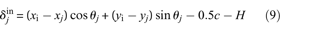
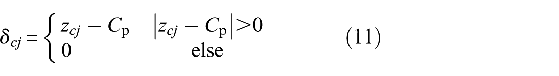
where x_o, x_i, and x_j denote the displacements of the outer race, inner race, and the j-th roller along the X-axis, respectively, while y_o, y_i, and y_j denote the displacements along the Y-axis. The term z_cj denotes the relative position between the roller and the center of the cage pocket hole, where $z_{c j} = 0.5 d_{m} (θ_{cage} - θ_{j})$ . In addition, the angular position of the cage is denoted as θ_cage, c denotes the radial internal clearance, C_p denotes the pocket clearance of the cage, and H denotes the time-varying displacement affecting the contact deformation of the races.

When outer ring defects occur, H = H_do, while when inner ring defects occur, H = H_di. When the roller fails, H = H_dro + H_dri. Force analysis is performed, and the kinetic differential equations for the inner and outer races are obtained.

{\begin{matrix} m_{i} {\overset{\cdot\cdot}{x}}_{i} + c_{s} {\overset{\cdot}{x}}_{i} + k_{s} x_{i} + \sum_{j = 1}^{N_{b}} β_{j} F_{k j}^{in} \cos θ_{j} - \sum_{j = 1}^{N_{b}} f_{k j}^{in} \sin θ_{j} = Q_{x} \\ m_{i} {\overset{\cdot\cdot}{y}}_{i} + c_{s} {\overset{\cdot}{y}}_{i} + k_{s} y_{i} + \sum_{j = 1}^{N_{b}} β_{j} F_{k j}^{in} \sin θ_{j} + \sum_{j = 1}^{N_{b}} f_{k j}^{in} \cos θ_{j} = Q_{y} \end{matrix}

(12)

{\begin{matrix} m_{o} {\overset{\cdot\cdot}{x}}_{o} + c_{h} {\overset{\cdot}{x}}_{o} + k_{h} x_{o} - \sum_{j = 1}^{N_{b}} β_{j} F_{k j}^{out} \cos θ_{j} + \sum_{j = 1}^{N_{b}} f_{k j}^{out} \sin θ_{j} = 0 \\ m_{o} {\overset{\cdot\cdot}{y}}_{o} + c_{h} {\overset{\cdot}{y}}_{o} + k_{h} y_{o} - \sum_{j = 1}^{N_{b}} β_{j} F_{k j}^{out} \sin θ_{j} - \sum_{j = 1}^{N_{b}} f_{k j}^{out} \cos θ_{j} = 0 \end{matrix}

(13)

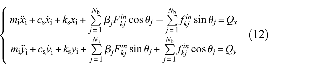
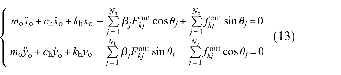
where m_i is the total mass of the shaft and inner race, while m_o donates the total mass of the housing and outer race. In addition, Q_x and Q_y denote the loads applied along the X-axis and Y-axis, respectively, while β_j represents the Heaviside function.⁴⁹

The kinetic differential equations of rollers are as follows:

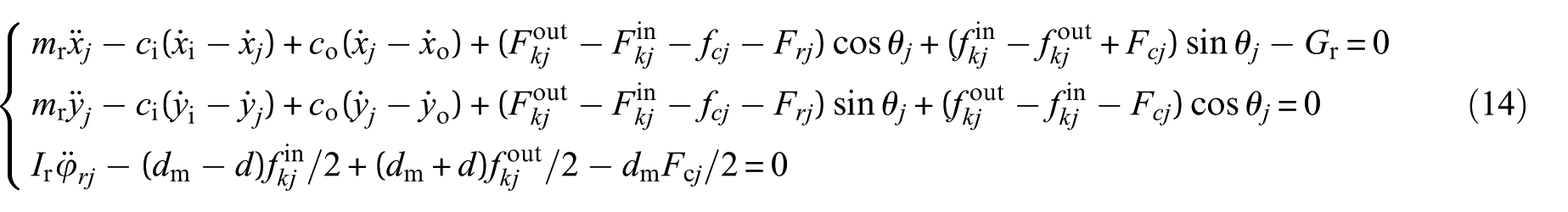
{\begin{matrix} m_{r} {\overset{\cdot\cdot}{x}}_{j} - c_{i} ({\overset{\cdot}{x}}_{i} - {\overset{\cdot}{x}}_{j}) + c_{o} ({\overset{\cdot}{x}}_{j} - {\overset{\cdot}{x}}_{o}) + (F_{k j}^{out} - F_{k j}^{in} - f_{c j} - F_{r j}) \cos θ_{j} + (f_{k j}^{in} - f_{k j}^{out} + F_{c j}) \sin θ_{j} - G_{r} = 0 \\ m_{r} {\overset{\cdot\cdot}{y}}_{j} - c_{i} ({\overset{\cdot}{y}}_{i} - {\overset{\cdot}{y}}_{j}) + c_{o} ({\overset{\cdot}{y}}_{j} - {\overset{\cdot}{y}}_{o}) + (F_{k j}^{out} - F_{k j}^{in} - f_{c j} - F_{r j}) \sin θ_{j} + (f_{k j}^{out} - f_{k j}^{in} - F_{c j}) \cos θ_{j} = 0 \\ I_{r} {\overset{\cdot\cdot}{φ}}_{r j} - (d_{m} - d) f_{k j}^{in} / 2 + (d_{m} + d) f_{k j}^{out} / 2 - d_{m} F_{c j} / 2 = 0 \end{matrix}

(14)

where m_r, F_rj, and ${\overset{\cdot\cdot}{φ}}_{rj}$ denote the mass, centrifugal force, and angular acceleration of the roller, respectively.

For the cage, the kinetic differential equations are:

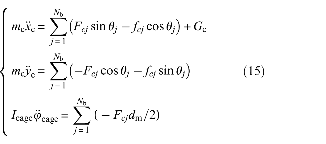
{\begin{matrix} m_{c} {\overset{\cdot\cdot}{x}}_{c} = \sum_{j = 1}^{N_{b}} (F_{c j} \sin θ_{j} - f_{c j} \cos θ_{j}) + G_{c} \\ m_{c} {\overset{\cdot\cdot}{y}}_{c} = \sum_{j = 1}^{N_{b}} (- F_{c j} \cos θ_{j} - f_{c j} \sin θ_{j}) \\ I_{cage} {\overset{\cdot\cdot}{φ}}_{cage} = \sum_{j = 1}^{N_{b}} (- F_{c j} d_{m} / 2) \end{matrix}

(15)

where x_c and y_c denote the displacement of the cage along the X-axis and Y-axis, respectively. Terms m_c, I_cage, and ${\overset{\cdot\cdot}{φ}}_{cage}$ represent the mass, rotational inertia, and angular acceleration of the cage.

Structural parameters are different in various bearing models. The proposed modeling method requires only structural, failure, and operational parameters as inputs to acquire a high fidelity DT model of the bearing. Specifically, the critical parameters such as contact stiffness k_in, k_out and damping c_i, c_o can be updated in real time by substituting fault parameters and real-time operating condition parameters into (3)–(8) based on available structural parameters. These parameters are employed in the force analysis of bearings to obtain the contact deformations of the rollers with the raceways and cage. Subsequently, the dynamic model of the bearing can be expressed as (12)–(15).

Verification of simulated signals

Effective DT models of rolling bearings aim to obtain simulated data reflecting the features of measured signals, thereby aiding in health status monitoring. To validate the DT model, the vibration response of NSK 6012 rolling bearings was collected under various fault states and operating conditions. Table 1 presents the detailed parameters of NSK 6012, and simulated vibration signals were obtained by applying the parameters to (12)–(15). Because the measured signal was collected at the shell, the simulated signal of the outer race was selected for comparative analysis.

Table 1.

Parameters of NSK 6012 bearings.

Parameters	Value
Contact angle, α (°)	0
Diameter of inner race, D_i (mm)	60
Diameter of outer race, D_o (mm)	95
Diameter of rollers, d (mm)	10.45
Pitch diameter, d_m (mm)	77.5
Number of rollers	12
Radial internal clearance, c (μm)	10

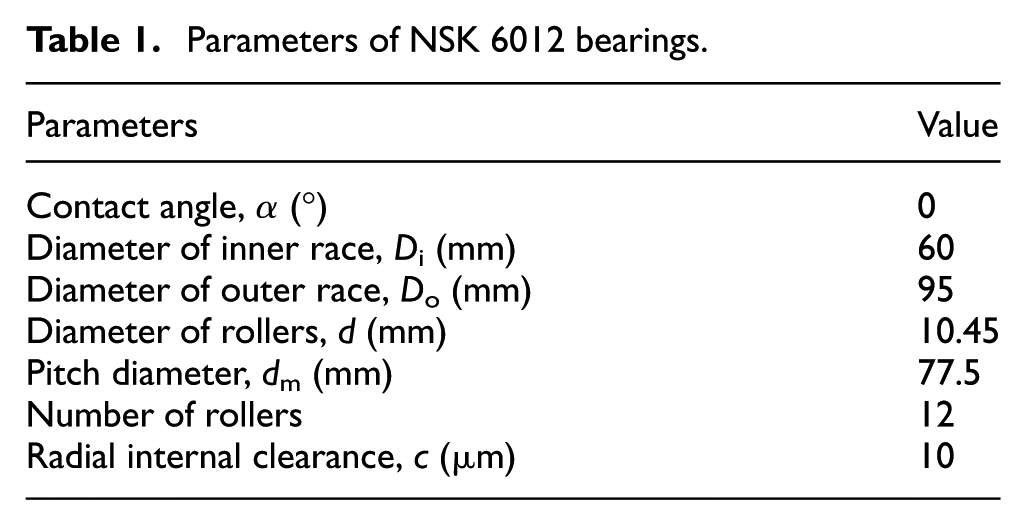
When the outer race fails (w_o = 1 mm), the bearing is subjected to a 1194 N load along the X-axis, and the rotational frequency of the inner race is f_s = 27.5 Hz. The roller passing frequency of the outer race is f_o = 142.75 Hz. The acceleration of the simulated and measured signals along the X-axis is presented in Figure 5(a) and (b), respectively. In the time domain, both the simulated and measured signals exhibit periodic impulses caused by the outer race fault, with an interval of Δ_o = 0.007 s, which corresponds to f_o. As illustrated in Figure 5(b) and (d), in the envelope spectra, the main frequency components of the simulated and measured signals are f_o and its harmonic components (2f_o, 3f_o, …).

Figure 5.

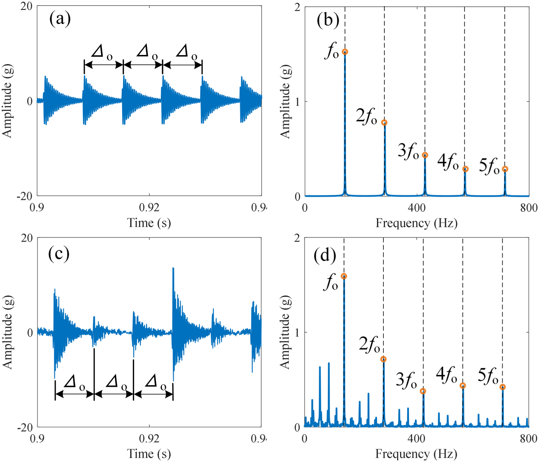
Accelerations with outer race faults along the X-axis. (a, c) Waveforms of simulated and measured data, respectively. (b, d) Envelope spectra of simulated and measured data, respectively.

Similarly, when the inner race fails with a fault size of w_i = 1 mm, the load is 856 N along the X-axis, and f_s = 38.33 Hz. The acceleration is presented in Figure 6(a) and (b). In the time domain, both the simulated and measured signals exhibit considerable modulation. Periodic impulses, occurring at intervals Δ_i (0.004 s) and Δ_s (0.026 s), are induced by the roller passing frequency of the outer race f_i (142.75 Hz) and f_s, respectively. The envelope spectra, illustrated in Figure 6(b) and (d), illustrate that apart from f_s, the main frequency components of both the simulated and measured signals are f_i and its harmonic components (2f_i, 3f_i, …).

Figure 6.

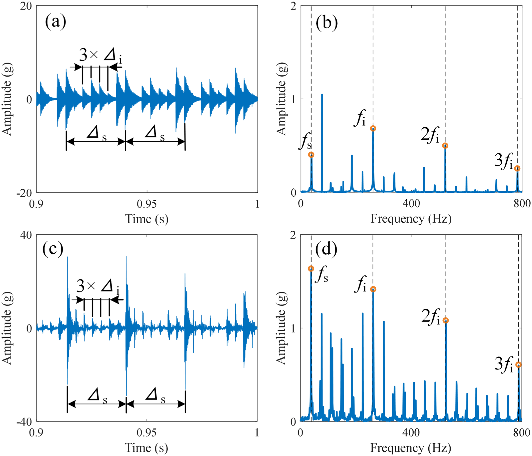
Accelerations with inner race faults along the X-axis. (a, c) Waveforms of simulated and measured data, respectively. (b, d) Envelope spectra of simulated and measured data, respectively.

The results indicate that simulated signals obtained from DT models, which are developed based on the structure and fault parameters of the bearings, effectively reflect the vibration characteristics of the measured signals in the time and frequency domains. This demonstrates the effectiveness of the proposed DT model and its ability to simulate bearing faults under various operating conditions.

Framework for imbalanced fault diagnosis

DFGAN is proposed to learn the mapping between the distributions of simulated and measured data, thereby reducing these discrepancies and enabling mutual conversion between simulated and measured samples. SEU-Nets are utilized as generators to optimize the performance of fault information extraction from simulated data. After training, simulated multisensor data are transformed into synthetic samples with a distribution similar to that of measured samples using the trained SEU-Net.

Principle of DFGAN

DFGAN is employed to transform simulated fault samples into synthetic samples with a data distribution similar to that of measured samples. As illustrated in Figure 7, DFGAN consists of two generators (G_s, G_m) and two discriminators (D_s, D_m). Both generators G_s and G_m utilize SEU-Net as a structural to achieve optimized extraction and deep fusion of fault features from the simulated samples. Both discriminators D_s and D_m utilize an identical Patch-GAN architecture.³¹

Figure 7.

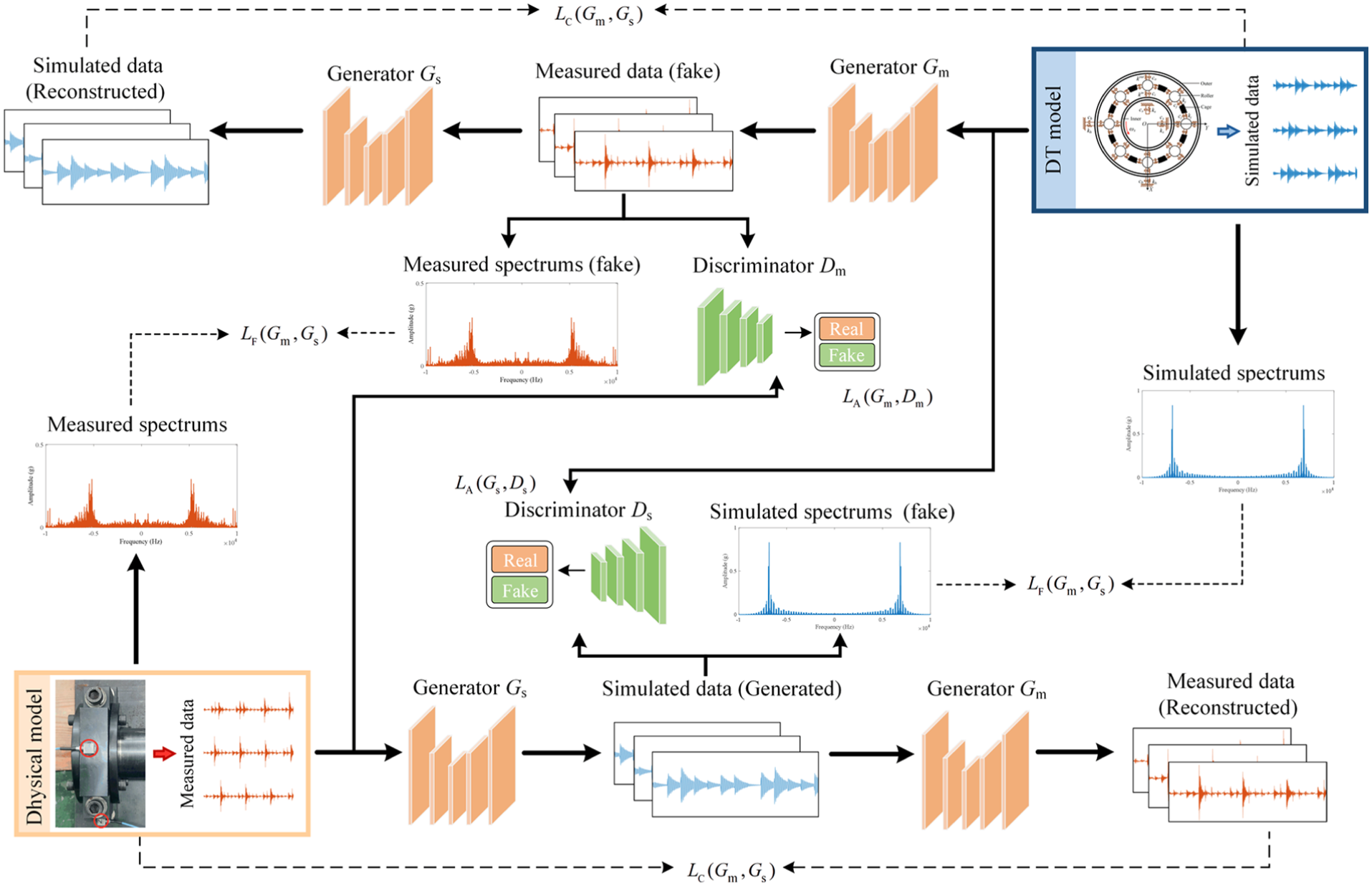
Architecture of DFGAN.

DFGAN is trained using a limited number of measured and simulated fault samples. Specifically, the first GAN consists of G_m and D_m, which facilitate the conversion of simulated samples x_s in the source domain S into the measured samples x_m in the target domain T. The generator G_m is utilized to learn fault features from the simulated samples x_s and generate synthetic samples G_m(x_s) of the measured signals x_m. Multiple feature fusion blocks in G_m extract and deeply fuse the fault features in x_s. Subsequently, feature weights are automatically obtained, and effective fault features are passed to G_m(x_s). As a result, the synthetic samples G_m(x_s) exhibit a data distribution similar to that of measured samples x_t in domain T, which can realize feature enhancement of measured samples x_m. The discriminator D_m differentiates the synthetic samples G_m(x_s) from the measured samples x_m, which opposes the training objective of G_m. Finally, the generator G_d attempts to map G_m(x_s) back to the domain S to ensure that G_m(x_s) retains the effective fault information in x_s. Similarly, the alternating training of G_s and D_s in the second GAN achieves the conversion of measured samples x_m into simulated samples x_s.

SEU-Nets for generators

Within DFGAN, SEU-Nets serve as generators, consisting of a down-sampling block, an up-sampling block, and feature fusion blocks. The structure and parameters of SEU-Net are illustrated in Figure 8(a). The down-sampling block reduces feature dimensions through three serially connected down-sampling layers. The up-sampling block restores feature dimensions using transposed convolutions, aiming to reconstruct features and generate synthetic samples. In addition, instance normalization (IN), dropout (DP), and rectified linear unit (ReLU) are utilized to enhance feature extraction and generalization ability of the network. Different from the existing generator structures, multiple feature fusion blocks are adopted in SEU-Net to realize the multilayer deep fusion of the feature maps from simulated signal x_s, as demonstrated in Figure 9. Feature fusion layers copy and concatenate down-sampled feature maps with their corresponding inputs in the up-sampling block in a multilayer based on the channel dimensions. With the purpose of fully retaining the fault information contained in the simulated signal x_s in synthetic samples, squeeze-and-excitation blocks are introduced as the attention module to prioritize critical features and compute channel-specific weights, allowing for multilayer deep feature fusion.⁵⁰ Specifically, global average pooling is utilized to process the input concatenated feature maps by compressing the spatial information of each channel into a scalar. Afterward, nonlinear dependencies between channels are learned by two fully connected (FC) operations to obtain channel weights. Finally, the channel weights are applied to the original feature map to weight critical feature channels and suppress irrelevant channels. This allows more effective fault information in the input samples to be retained in the fake samples, thus improving the accuracy of sample reconstruction, and preserving detailed features.

Figure 8.

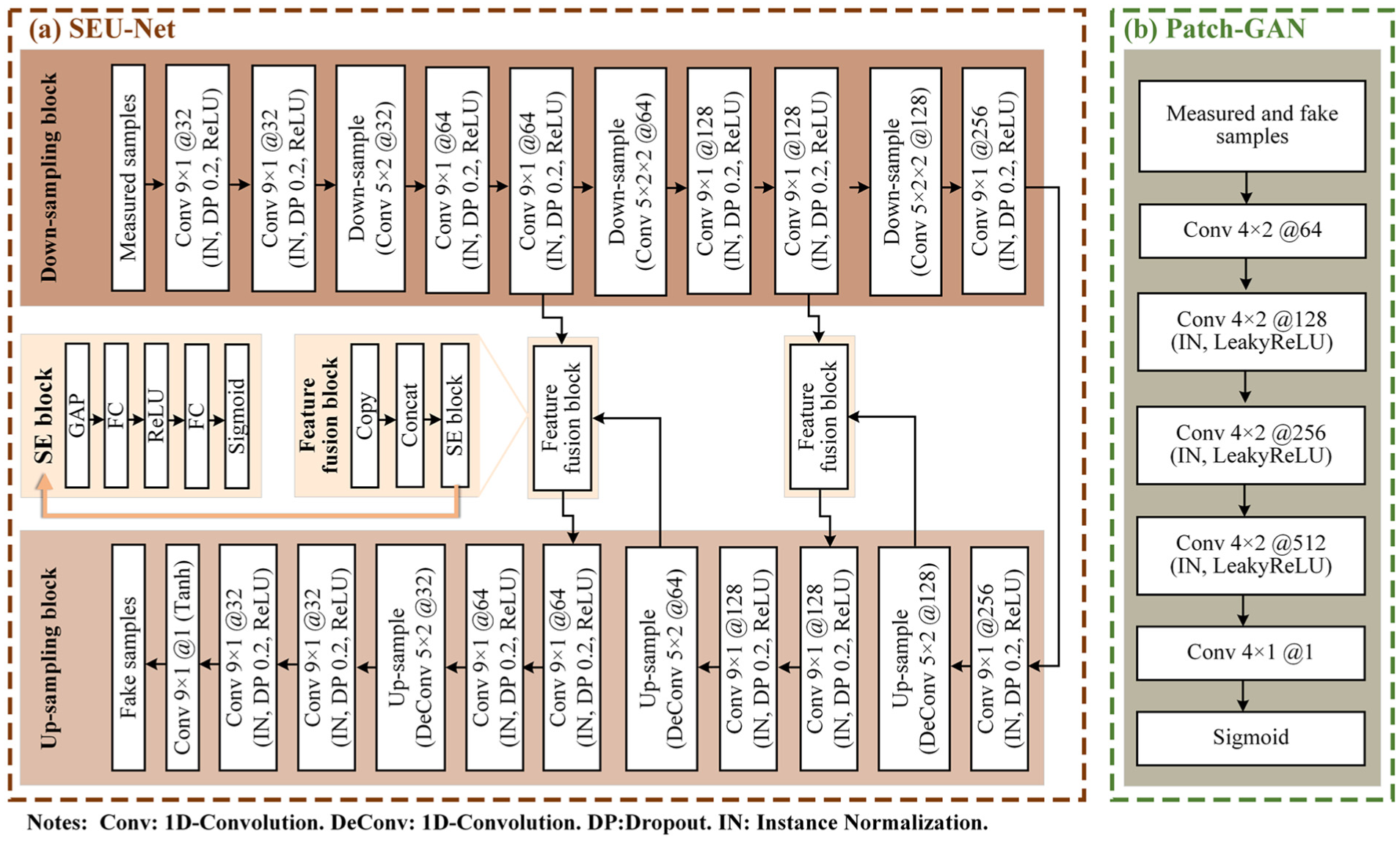
(a) Structure and parameters of the SEU-Net generator. (b) Structure and parameters of the Path-GAN discriminator.

Figure 9.

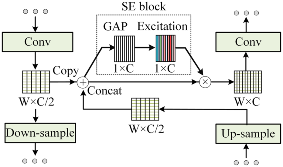
Diagram of the feature fusion block.

Patch-GAN for discriminators

Patch-GAN can better focus on the local features of input samples than traditional GAN discriminators. Therefore, Patch-GANs are used as discriminators. Figure 8(b) presents the structure and parameters of the discriminators, which serve to discriminate between synthetic samples. The elements in the output matrix are converted to values between 0 and 1 by the sigmoid activation function. These values represent the probability that different regions of the input data correspond to real samples.

The loss function with spectral correlation loss of the DFGAN

Frequency-domain analysis reveals the intensity of the signal over different frequency components, which are not directly captured by time-domain analysis. However, loss functions are generally designed in existing data generation methods based only on the time series data of samples, resulting in the lack of explicit constraints on frequency-domain features. Moreover, there may still exist large discrepancies between synthetic and measured samples in the frequency domain. Thus, a loss function called spectral correlation loss (L_F) is designed following the Pearson’s correlation of the spectra to curtail these discrepancies. Pearson’s correlation is a crucial indicator for evaluating the similarity between two sets of data. The closer the Pearson’s correlation coefficient between samples is to 1, the higher the consistency of the data distribution. Unlike existing methods, L_F utilizes the correlation coefficient to constrain the spectral data distribution of the synthetic samples, so as to achieve the alignment of the frequency distributions of the synthetic and measured samples. The Pearson’s correlation coefficient can be calculated as follows:

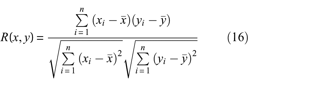
R (x, y) = \frac{\sum_{i = 1}^{n} (x_{i} - \bar{x}) (y_{i} - \bar{y})}{\sqrt{\sum_{i = 1}^{n} {(x_{i} - \bar{x})}^{2}} \sqrt{\sum_{i = 1}^{n} {(y_{i} - \bar{y})}^{2}}}

(16)

where x and y denote two samples containing the same number of points.

DFGAN is designed to learn the bidirectional mapping relationship between simulated samples x_s and measured samples x_m, realizing the interconversion of samples in domain T and sample in domain S. Therefore, the composition of spectral correlation loss L_F should be considered in two parts: (1) the linear correlation between the spectrums of G_m(x_s) and measured sample x_m; (2) the linear correlation between the spectrums of G_s(x_m) and simulated sample x_s. L_F needs to constrain both the domain S to T and the domain T to S conversion process simultaneously. Considering the correlation coefficients between the spectra of the synthetic samples generated by G_m and G_s and the spectra of the measured samples, the spectral correlation loss of DFGAN is obtained as follows:

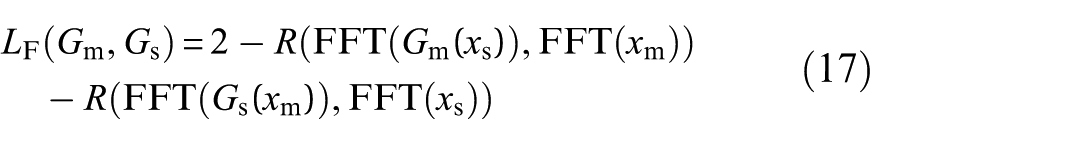
\begin{matrix} L_{F} (G_{m}, G_{s}) = 2 - R (FFT (G_{m} (x_{s})), FFT (x_{m})) \\ - R (FFT (G_{s} (x_{m})), FFT (x_{s})) \end{matrix}

(17)

where FFT(·) denotes the complex representation of data in the frequency domain.

The adversarial losses L_A(G_m, G_d) and L_A(G_s, G_s) are utilized to ensure that the generated synthetic samples match the data distribution in T:

L_{A} (G_{m}, D_{m}) = E_{x_{m} ~ T} [{(D_{m} (x_{m}) - 1)}^{2}] + E_{x_{s} ~ S} [D_{m} {(G_{m} (x_{s}))}^{2}]

(18)

L_{A} (G_{s}, D_{s}) = E_{x_{s} ~ S} [{(D_{s} (x_{s}) - 1)}^{2}] + E_{x_{m} ~ T} [D_{s} {(G_{s} (x_{m}))}^{2}]

(19)

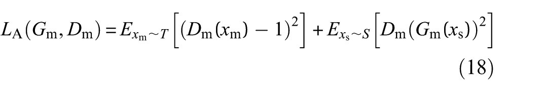
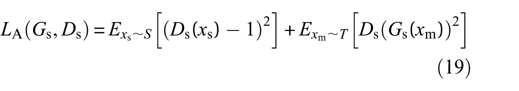
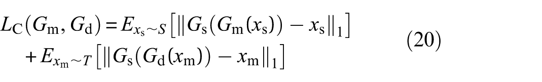
where $E_{x_{m} ~ T}$ is the expectation of the measured sample x_m in T, and $E_{x_{s} ~ S}$ denotes the expectation of the simulated sample x_s in S.

The cycle-consistency loss L_C(G_m, G_d) is introduced to constrain the training of generators G_m and G_d:

\begin{matrix} L_{C} (G_{m}, G_{d}) = E_{x_{s} ~ S} [{‖ G_{s} (G_{m} (x_{s})) - x_{s} ‖}_{1}] \\ + E_{x_{m} ~ T} [{‖ G_{s} (G_{d} (x_{m})) - x_{m} ‖}_{1}] \end{matrix}

(20)

To allow the generators to extract and retain fault features from input samples, identity-mapping loss is introduced, which helps to reduce the migration of irrelevant features:

L_{I} (G_{m}, G_{s}) = E_{x_{m} ~ T} [{‖ G_{m} (x_{m}) - x_{m} ‖}_{1}] + E_{x_{s} ~ S} [{‖ G_{s} (x_{s}) - x_{s} ‖}_{1}]

(21)

In summary, the objective function of DFGAN during training can be expressed as follows:

\begin{matrix} L = L_{A} (G_{m}, D_{m}) + L_{A} (G_{s}, D_{s}) + λ_{c} L_{c} (G_{m}, G_{s}) \\ + λ_{I} L_{I} (G_{m}, G_{s}) + λ_{F} L_{F} (G_{m}, G_{s}) \end{matrix}

(22)

where λ_C, λ_I, and λ_F represent the trade-off parameters of L_C, L_I, and L_F, respectively.

MCNN for fault diagnosis

To effectively utilize fault information from multisensor data and enhance the accuracy of bearing diagnosis, MCNN is proposed as the classifier for feature extraction and fusion of multisensor data. The parameters and structure of MCNN are presented in Figure 1 and Table 2. The architecture incorporates multibranch CNNs, with the number of branches corresponding to the number of sensors. In feature extraction, batch normalization (BN), and ReLU operations are performed sequentially following each convolution to optimize the feature extraction of MCNN.

Table 2.

Structure of each branch of MCNN.

Layers	Kernel (size/stride)	Output size	Operation
Conv 1	15/4	16 × 512	BN + ReLU
Pool 1	2/2	16 × 256	/
Conv 2	3/2	32 × 128	BN + ReLU
Pool 2	2/2	32 × 64	/
Covn 3	3/2	64 × 32	BN + ReLU
Pool 3	2/2	64 × 16	/
Covn 4	3/2	128 × 8	BN + ReLU
Pool 4	2/2	128 × 4	/
Fusion	/	2048	/
FC 1	/	512	/
FC 2	/	128	/
FC 3	/	Classes	softmax

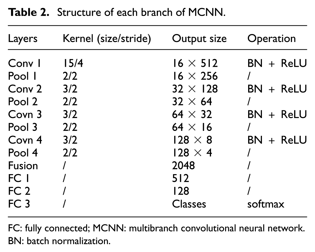
FC: fully connected; MCNN: multibranch convolutional neural network. BN: batch normalization.

Multisensor data are fed into individual branch CNNs to extract the corresponding fused features. Subsequently, three FC layers with softmax are utilized to achieve fault diagnosis based on the fused features. Cross-entropy loss is employed to evaluate diagnostic performance.

Experiment and analysis

The code for the proposed method is implemented using the PyTorch 2.1 developed by Facebook AI Research (FAIR) and written in Python 3.8 developed by Python Software Foundaton (PSF). To minimize the influence of random factors, all experiments were repeated 10 times, and the model performance was evaluated based on the average diagnostic accuracy.

Training details

The hyperparameters of DFGAN and MCNN were set by parameter fine-tuning to fully utilize the performance of the proposed method. Concerning both DFGAN and MCNN, the Adam optimizer was selected as the adaptive optimization algorithm to update model parameters and accelerate network convergence. The learning rate lr should be dynamically updated to match the gradient descent process of the loss function. In DFGAN, the lr of generators G_m and G_s and discriminators D_m and D_s, where the lr decreased from 0.0005 to 0.0001, were updated by the cosine-annealing algorithm to avoid local minima and find the global optimum. Additionally, the weight parameter λ_F of the L_F was set at 1 to constrain the frequency distribution of the synthetic samples. The training iterations of DFGAN were set at 4000 to ensure the stable generation of synthetic samples. In MCNN, to determine the optimal solution for classification task, the initial lr of MCNN was set to 0.0002 and reduced by 80% every 20 iterations. The training iterations were set to 120 with a batch size of 128 to avoid overfitting of the diagnostic model.

Methods for comparison

To evaluate the performance of DFGAN for imbalanced fault diagnosis of rolling bearings, five methods were selected for comparison. The diagnostic models for all comparison methods are the same as for DFGAN.

MCNN¹⁶: Without sample augmentation, raw imbalanced data is fed into the diagnostic model, and multisensor data features are extracted by a multibranch CNN, used as a baseline.

DCGAN⁵¹: It serves as a data generation model. A deep CNN is used as a generator for synthesizing fault samples.

LSGAN⁵²: It serves as a data generation model. Least squares loss is employed to optimize model training.

WGAN-GP³¹: It serves as a data augmentation method. WGAN-GP uses the Wasserstein distance as a loss function. The Lipschitz constraint is forced to be satisfied by the gradient penalty to increase the stability of model training.

CycleGAN⁵³: CycleGAN is used to learn the mapping between simulated samples from the DT model and measured samples and synthesize fault samples, so as to synthesize fault samples. It is an effective sample augmentation method.

Case1: Case Western Reserve University (CWRU) dataset

Description and processing of dataset

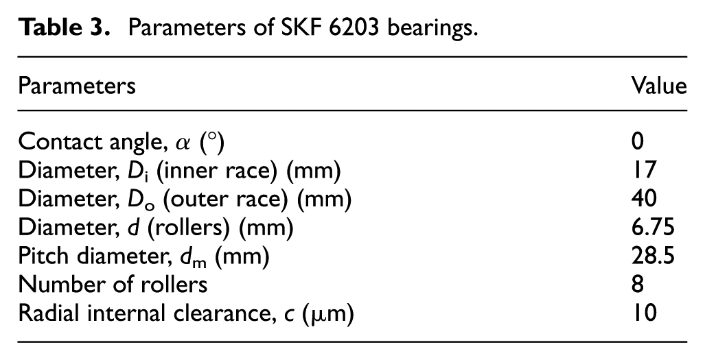
The structure of the test bench corresponding to the CWRU dataset is presented in Figure 10. Accelerometers were placed on the fan end (FE) and drive end (DE) of the motor housing. An SKF 6203 rolling bearing was employed to support the FE, with its parameters presented in Table 3. To simulate the health conditions of the FE, faults were introduced separately on the roller, outer race, and inner race of the 6203 bearings, with three fault sizes: 0.007, 0.014, and 0.021 in. Therefore, including the normal state, the 6203 bearing had a total of 10 health conditions. Under the 3-hp operating condition, faults on the outer race were located at the 3 o’clock position. This study employed vibration data from the FE and DE sensors for processing and analysis to simulate imbalanced multisensor data.

Figure 10.

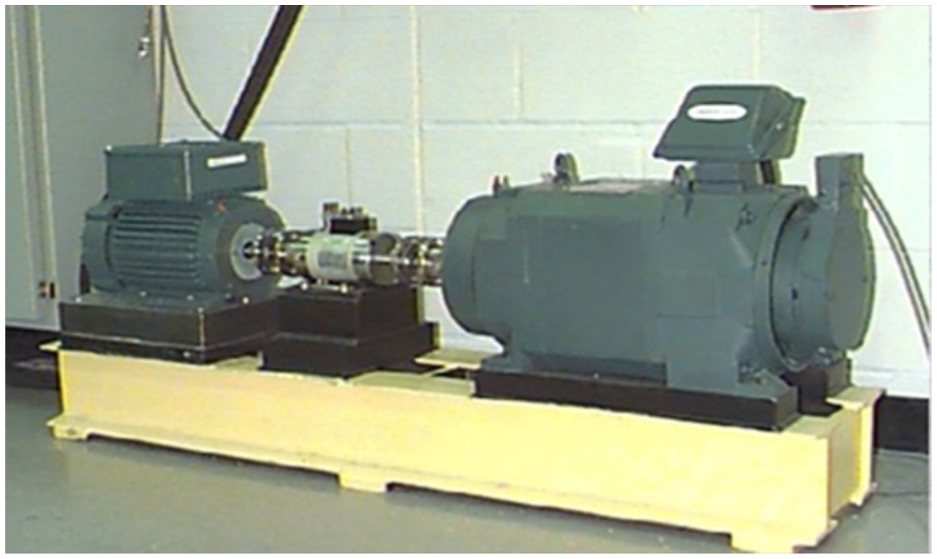
The test bench of Case Western Reserve University (CWRU) dataset.

Table 3.

Parameters of SKF 6203 bearings.

Parameters	Value
Contact angle, α (°)	0
Diameter, D_i (inner race) (mm)	17
Diameter, D_o (outer race) (mm)	40
Diameter, d (rollers) (mm)	6.75
Pitch diameter, d_m (mm)	28.5
Number of rollers	8
Radial internal clearance, c (μm)	10

Using the fault parameters as inputs, the DT model of the 6203 rolling bearing with multiple DOFs was developed using (12)–(15). The simulated and measured data were processed using a sliding window technique for both the DE and FD sensors.⁵ For each health condition, the vibration data were divided into 400 measured samples, each containing 2048 consecutive points. However, fault samples are generally difficult to obtain in applications, and the difference in the number of samples affects the reliability of the diagnostic model. Therefore, it is necessary to investigate the performance of DFGAN for data synthesis under extreme imbalanced data. In this section, only two measured samples from the DE and FD sensors were randomly selected to perform DFGAN training under each fault condition. Meanwhile, 300 samples under normal conditions were used as the majority class to simulate the data distribution in industrial scenarios. In this way, the ratio of each fault condition to the normal condition sample (imbalance ratio) reaches 1:150, forming extremely imbalanced data. Then, the imbalanced data were augmented with synthetic samples obtained from DFGAN. Consequently, the number of samples in each fault class was equal to that of the normal class. The augmented data were utilized to implement bearing fault diagnosis. Therefore, the training set included 300 samples (298 synthetic and 2 measured) from each sensor (excluding the normal state). The testing set for each health condition consisted of 100 real samples from each of the DE and FD sensors. The dataset is presented in Table 4.

Table 4.

The datasets for DE and FE sensors.

Fault type	Fault size (inches)	Training set		Testing set	Sample class
Fault type	Fault size (inches)	Measured	Synthetic	Testing set	Sample class
B	0.007	2	298	100	0
B	0.014	2	298	100	1
B	0.021	2	298	100	2
IR	0.007	2	298	100	3
IR	0.014	2	298	100	4
IR	0.021	2	298	100	5
OR	0.007	2	298	100	6
OR	0.014	2	298	100	7
OR	0.021	2	298	100	8
Normal	/	300	0	100	9

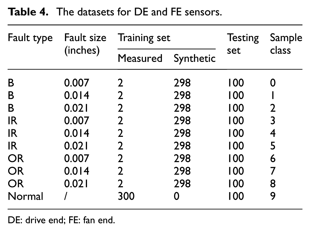
DE: drive end; FE: fan end.

Evaluation of synthetic samples

The data from the FE sensor are selected for analysis in this section to validate the synthetic samples obtained with DFGAN in each fault class on the CWRU dataset. As observed from Figure 11, the waveforms and spectrums of the synthetic samples were compared with those of the measured samples. Bearing faults induced periodic impulses in the waveforms. The synthetic and measured samples in each fault class demonstrated similar time-domain waveforms with the same intervals of impulses. In other words, the synthetic samples can accurately reflect the fault features of the measured samples in the time domain. In the frequency domain, the Pearson’s correlation coefficients Corr between the spectrums of the synthetic and the measured samples in each fault class reached more than 0.7, implying that the synthetic samples accurately reconstructed the frequency components of the measured samples. This also verified the validity of the L_F on the CWRU dataset.

Figure 11.

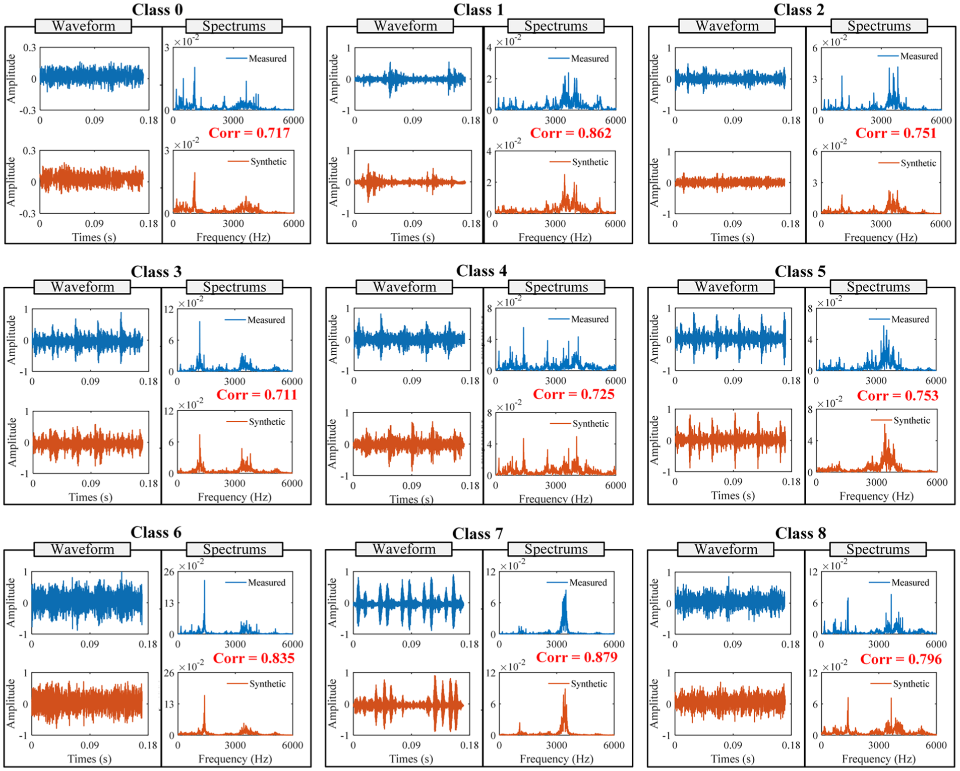
Waveforms and spectrums of the synthetic and measured samples corresponding to the FE sensor.

The quality of the synthesized samples is quantitatively analyzed. Maximum mean discrepancy (MMD) determines whether samples originate from the same data distribution by calculating their mean difference in a high-dimensional space.³⁰ A lower MMD value indicates a higher-quality synthetic sample. Using data from the FE sensor as an example, the MMD values of the synthetic samples obtained from different methods are displayed in Table 5. In most health conditions, the MMD value between the synthetic samples obtained from DFGAN and the measured samples is the lowest, indicating that the synthetic samples are of higher quality.

Table 5.

The MMD values of the synthetic samples corresponding to the FE Sensor.

Classes	Methods
	DFGAN	CycleGAN	DCGAN	LSGAN	WGAN-GP
0	0.058	0.163	3.984	4.191	1.287
1	0.119	0.113	1.666	1.654	1.827
2	0.048	0.232	1.377	1.385	1.446
3	0.073	0.769	1.560	1.506	1.623
4	0.056	0.658	1.218	1.458	1.432
5	0.057	0.293	1.376	1.269	1.317
6	0.128	0.818	5.418	1.254	1.436
7	0.087	0.123	1.388	1.558	1.237
8	0.074	0.769	1.379	1.629	1.222

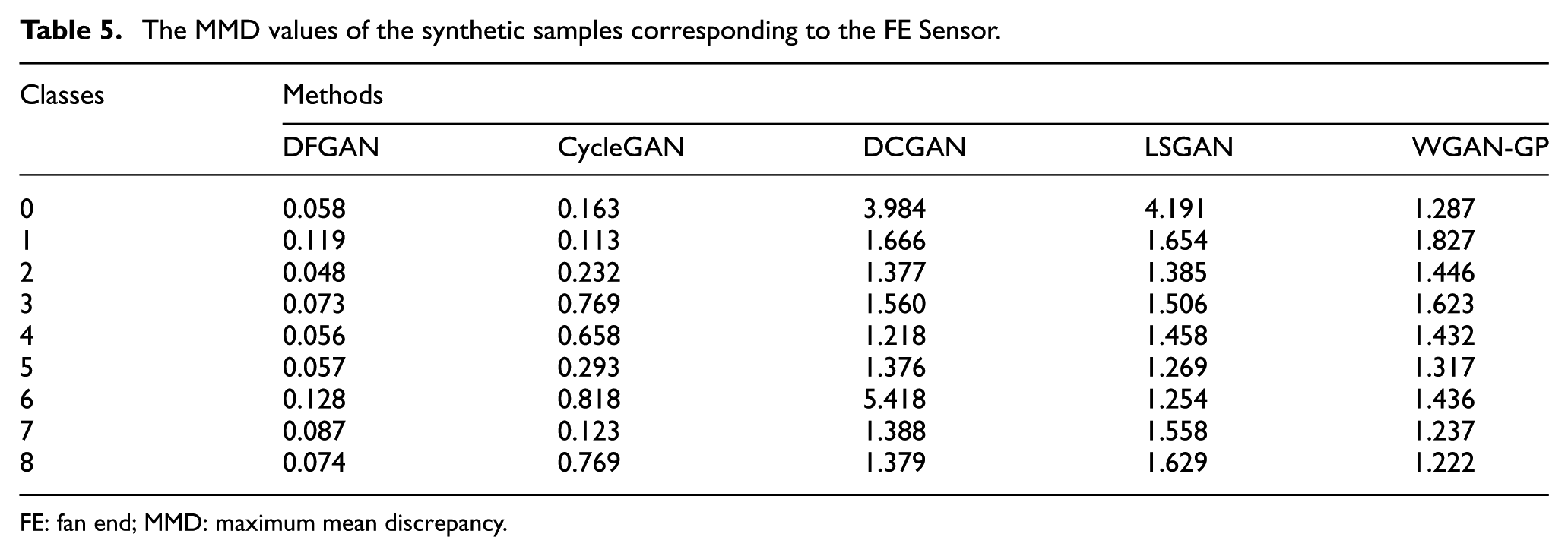
FE: fan end; MMD: maximum mean discrepancy.

Experimental results and discussion

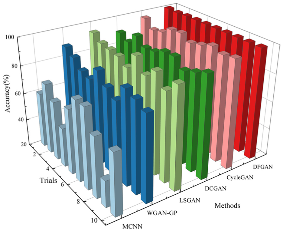
The performance of the different methods was evaluated using the test samples, with the diagnostic results displayed in Figure 12 and Table 6. With a limited number of measured fault samples, MCNN achieved an average diagnostic accuracy of only 63.24%. Through DTs, DFGAN achieved a diagnostic accuracy of 99.96%, an improvement of 36.72% over MCNN. This reflects that simulated fault information from DT models helps improve the imbalanced fault diagnostic performance of bearings. In addition, WGAN-GP, LSGAN, DCGAN, and CycleGAN all enhanced the imbalanced multisensor data, exhibiting better performance than MCNN, with an average diagnostic accuracy of 82.66%, 89.65%, 90.70%, and 95.88%, respectively. Compared with the comparison methods, the DFGAN achieved the highest average diagnostic accuracy on the CWRU dataset, outperforming WGAN-GP, LSGAN, DCGAN, and CycleGAN by 17.30%, 10.31%, 9.26%, and 4.08%, respectively. The diagnostic results demonstrate the superiority of DFGAN. The standard deviation (SD) of the accuracy over 10 trials demonstrates the stability of the model. With a SD value of just 0.001, the proposed method exhibits superior stability than comparison methods. As suggested in Table 6, statistical analysis was performed on the diagnostic results. The 95% confidence intervals (CI) of different methods were calculated to verify the robustness of the proposed method. The 95% CI for DFGAN is [99.87, 100], which is the narrowest and does not overlap with those of the comparison methods. Hence, the performance improvements achieved by DFGAN are statistically significant with excellent robustness.

Figure 12.

Diagnosis results for CWRU dataset.

Table 6.

Diagnosis accuracy for CWRU dataset.

Methods	Accuracies
	Ave	Max	Min	SD	95% CI
MCNN	63.24	78.00	39.00	0.121	[54.53, 71.95]
WGAN-GP	82.66	88.90	75.40	0.045	[79.27, 86.05]
LSGAN	89.65	94.30	83.80	0.039	[86.71, 92.59]
DCGAN	90.70	93.80	86.40	0.027	[88.73, 92.67]
CycleGAN	95.88	98.00	90.80	0.026	[94.00, 97.76]
DFGAN	99.96	100	99.60	0.001	[99.87, 100]

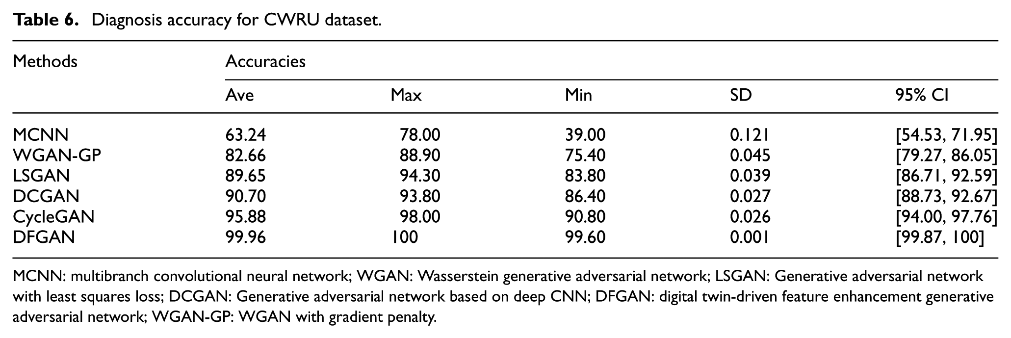
MCNN: multibranch convolutional neural network; WGAN: Wasserstein generative adversarial network; LSGAN: Generative adversarial network with least squares loss; DCGAN: Generative adversarial network based on deep CNN; DFGAN: digital twin-driven feature enhancement generative adversarial network; WGAN-GP: WGAN with gradient penalty.

The diagnostic results were visualized for further analysis, with the confusion matrices of the different methods displayed in Figure 13. Due to insufficient fault samples, MCNN achieved a diagnostic accuracy of over 80% only for classes 1, 2, 3, and 9. Given the low quality of the generated samples, the diagnostic accuracy of WGAN-GP for classes 2, 3, and 5 was only 69%, 70%, and 73%, respectively. As displayed in Figure 13(c) and (d), LSGAN and DCGAN achieved diagnostic accuracy of 48% and 70% for class 3, and the corresponding values for class 5 were 70% and 63%, respectively. In other words, neither LSGAN nor DCGAN can accurately identify samples from classes 3 and 5. In addition, CycleGAN identified 20% of class 0 samples as class 2. As illustrated in Figure 13(f), the highest diagnostic accuracy was achieved by DFGAN for all health conditions, further demonstrating the superiority of the proposed method.

Figure 13.

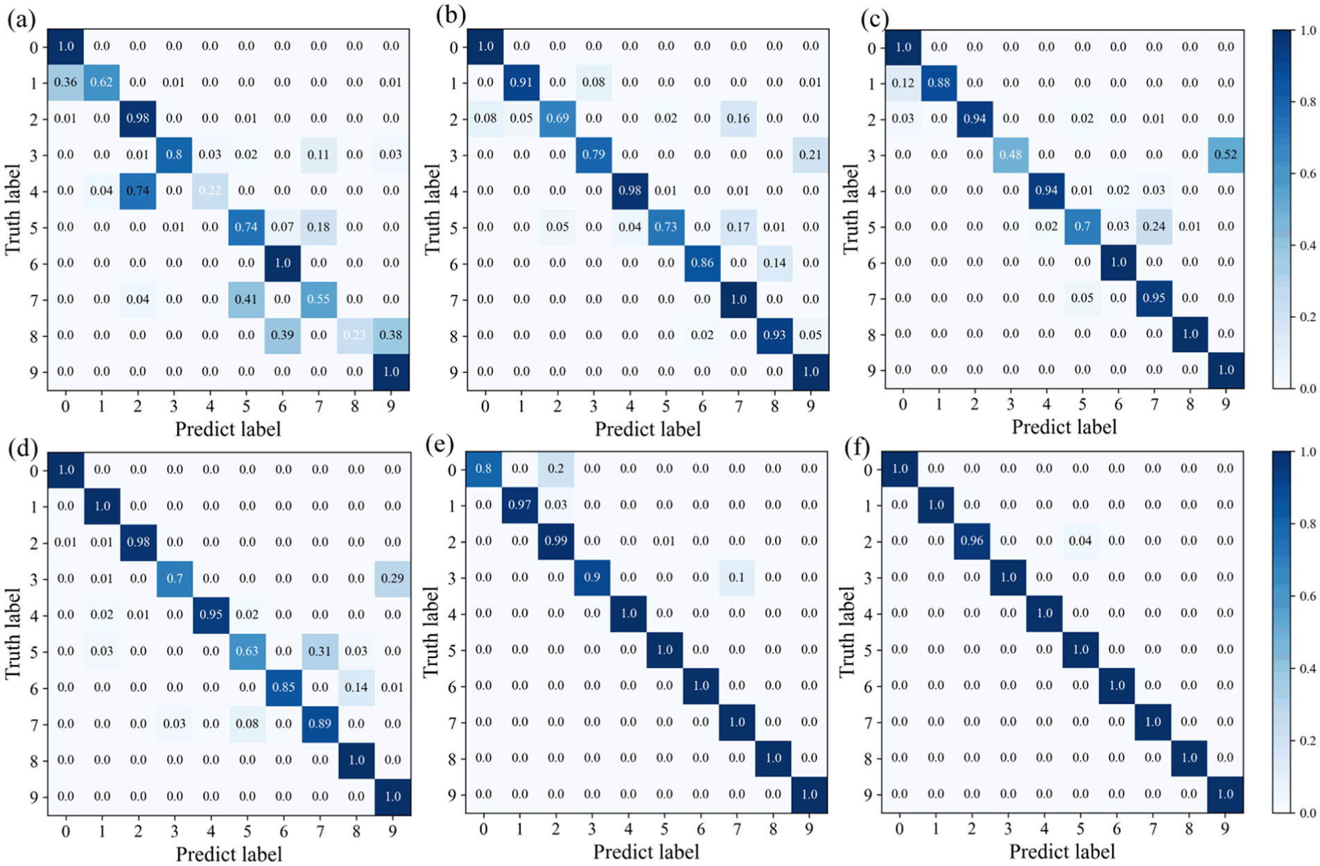
Confusion matrices for CWRU dataset: (a) MCNN, (b) WGAN-GP, (c) LSGAN, (d) DCGAN, (e) CycleGAN, and (f) DFGAN.

Analysis of synthetic samples with different number

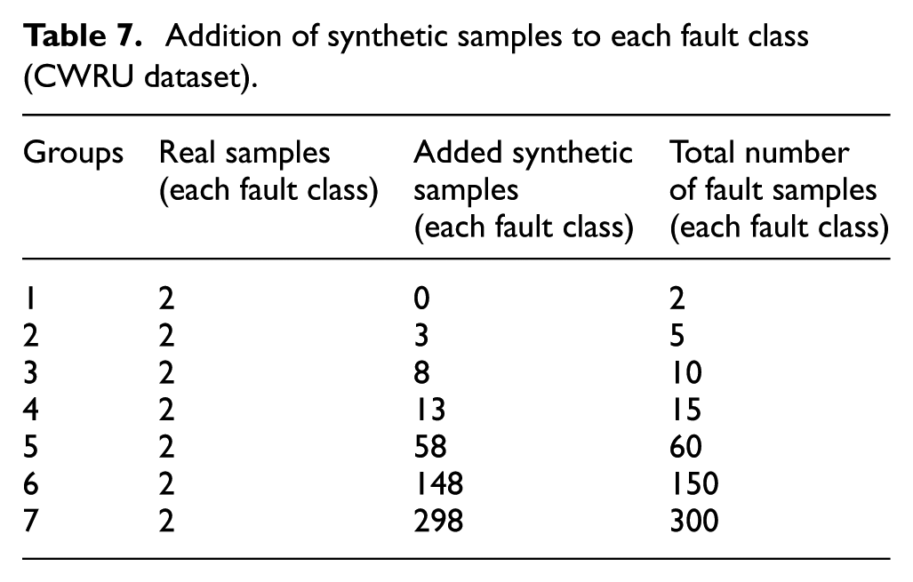
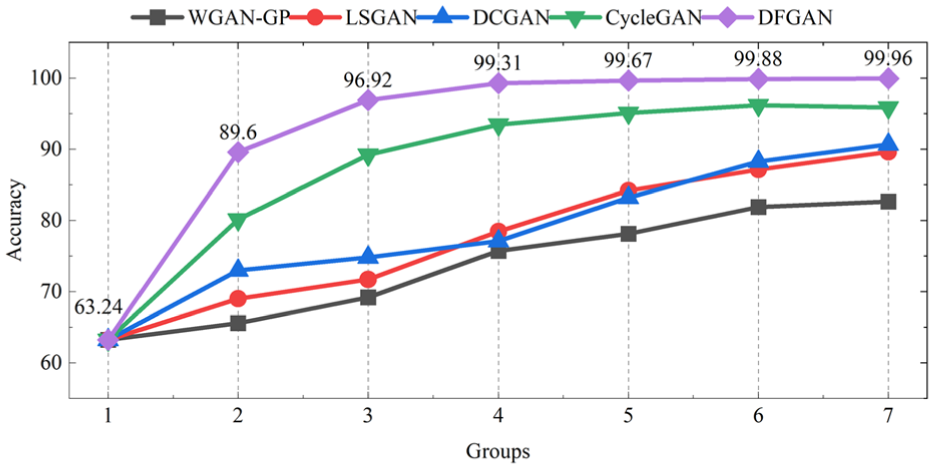
Sufficient samples in each health condition are essential for the diagnostic model to extract fault features and achieve reliable diagnostic results. In fault diagnosis, the difference in the number of normal and fault samples may introduce bias to the diagnostic model. As revealed in Table 7, the effect of the number of fault samples on the diagnostic performance was investigated by adding different numbers of synthetic fault samples to each fault class (Class 0–Class 9), which gradually restores the imbalanced data to the balanced state. The experimental setup is the same as in Section “Experimental results and discussion.” The diagnostic results are exhibited in Figure 14.

Table 7.

Addition of synthetic samples to each fault class (CWRU dataset).

Groups	Real samples (each fault class)	Added synthetic samples (each fault class)	Total number of fault samples (each fault class)
1	2	0	2
2	2	3	5
3	2	8	10
4	2	13	15
5	2	58	60
6	2	148	150
7	2	298	300

Figure 14.

Diagnostic results with different numbers of synthetic samples added to each fault class (CWRU dataset).

Table 7 and Figure 14 reflect that the diagnostic accuracy corresponding to all methods increases as the number of synthetic samples increases. After 3, 8, 13, 58, 148, and 297 synthetic samples were added for each fault class, the proposed method achieved 89.60%, 96.92%, 99.31%, 99.67%, 99.6%, and 99.96% diagnostic accuracy, respectively. After the total number of fault samples for each fault class reached 15, the performance of the proposed method tended to stabilize, with diagnostic accuracies all over 99%. Compared to the comparison methods, the proposed method reached the highest diagnostic accuracy under the addition of different synthetic samples, demonstrating the superiority of the proposed method.

Case2: Self-built (AHU) dataset

Description and processing of dataset

The effectiveness of the proposed method is also verified by the dataset obtained from the self-built test bench (AHU dataset). The structure and parameters of test bench are displayed in Figure 15 and Table 1. To simulate different health conditions, faults were introduced separately on the inner and outer races. In addition, a multifault was simulated by introducing faults on the roller and inner race simultaneously. Vibration signals were acquired via accelerometers mounted in the horizontal and vertical directions of the test bearings, with a sampling frequency of 20 kHz.

Figure 15.

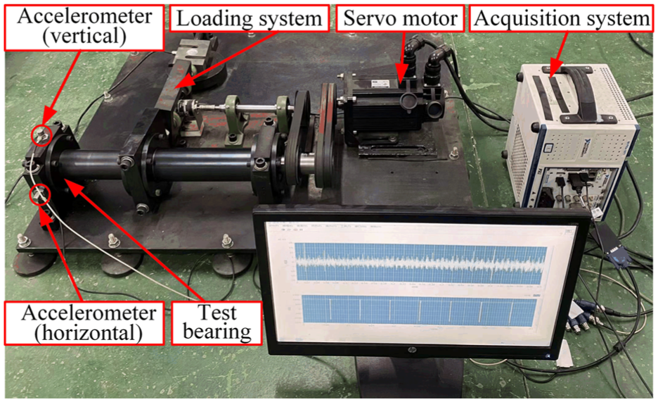
Structure of the test bench for NSK 6012 bearing.

As in Case 1, the dataset was split using the sliding window method, with each sample containing 2048 consecutive data points. Two measured samples from the vertical accelerometer (VA) and horizontal accelerometer (HA) were randomly selected to train DFGAN to generate synthetic samples. Therefore, as illustrated in Table 8 for each health condition, the training set consisted of 298 synthetic samples and 2 measured samples per sensor, except for the normal state.

Table 8.

Datasets for VA and HA accelerometers.

Fault type	Fault size (mm)	Training set		Testing set	Sample class
		Measured	Synthetic
IR	0.5	2	298	100	0
IR	1.0	2	298	100	1
IR	2.0	2	298	100	2
MF	0.5	2	298	100	3
MF	1.0	2	298	100	4
MF	2.0	2	298	100	5
OR	0.5	2	298	100	6
OR	1.0	2	298	100	7
OR	2.0	2	298	100	8
Normal	/	300	0	100	9

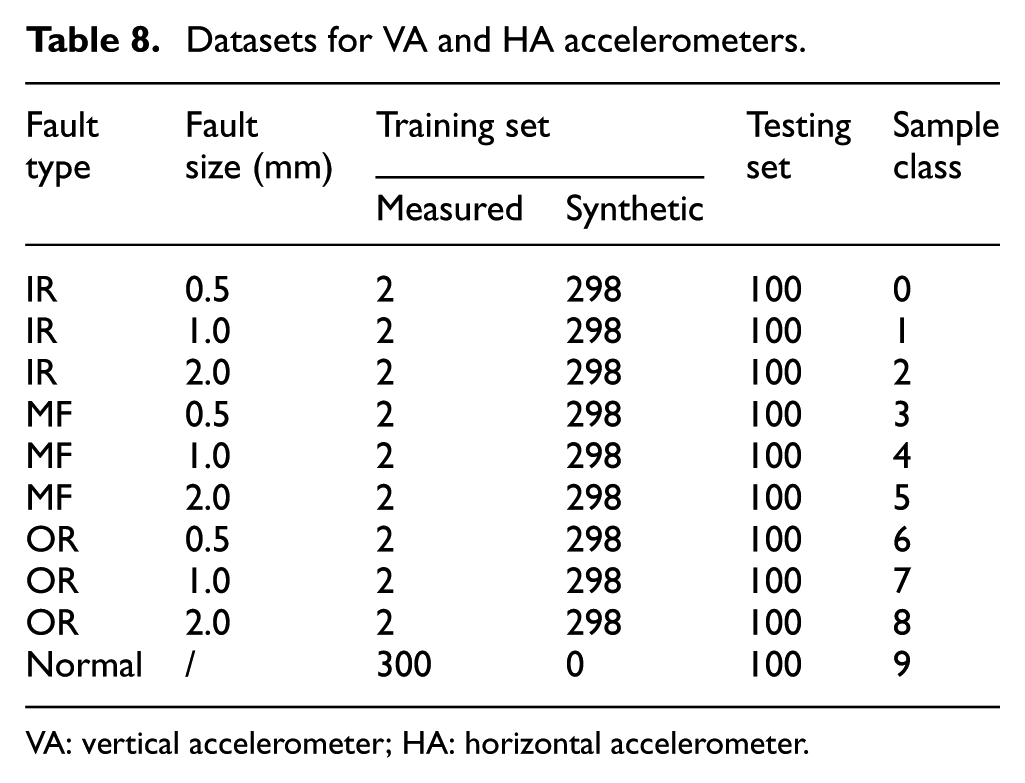
VA: vertical accelerometer; HA: horizontal accelerometer.

Evaluation of synthetic samples

In this section, the quality of the synthetic samples is assessed by analyzing the data from the VA accelerometer on the AHU dataset. As observed from Figure 16, the waveforms and spectrums of the synthetic samples were compared with those of the measured samples. In the time domain, bearing faults induced obvious periodic impulses in the waveforms. It can be obviously that both the synthetic and the measured samples have similar time-domain waveforms and the same intervals of impulses in each fault class, which indicates that the synthetic samples can accurately reflect the time-domain fault features of the measured samples. In the frequency domain, the Pearson’s correlation coefficients Corr between the spectrums of the synthetic and the measured samples in each fault class reach more than 0.7, which indicates that the synthetic samples accurately reconstruct the frequency components of the measured samples, and proves the validity of the L_F on the AHU dataset.

Figure 16.

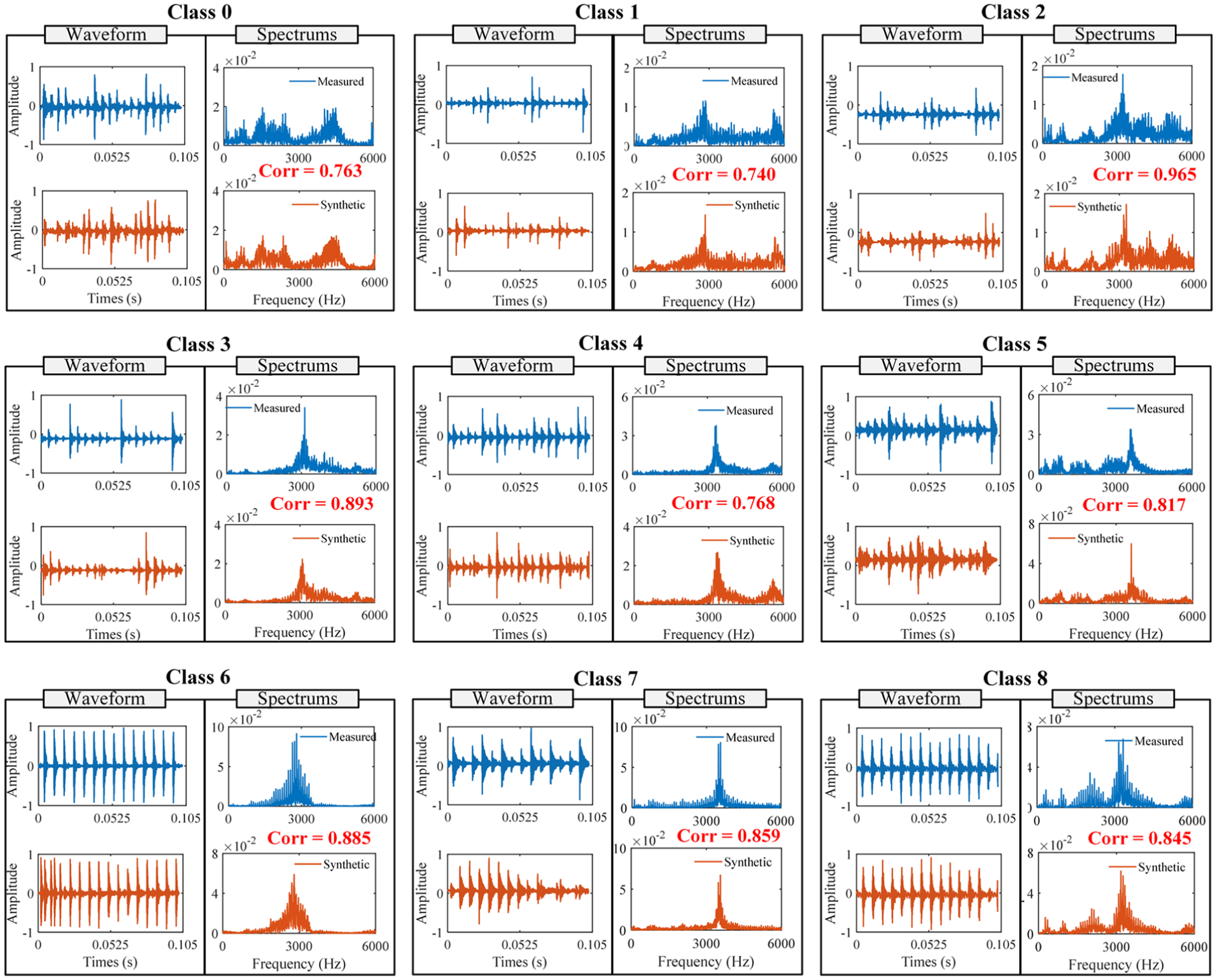
Waveforms and spectrums of synthetic and measured samples corresponding to VA accelerometers.

To assess the quality of the synthetic samples, data from the VA sensor were employed to generate synthetic samples by WGAN-GP, LSGAN, DCGAN, CycleGAN, and DFGAN. The MMD values between the synthetic and real samples are presented in Table 9. The synthetic samples generated by DFGAN exhibited the lowest MMD values for all fault conditions, indicating that their data distribution was closest to that of the measured samples.

Table 9.

MMD values of synthetic samples corresponding to VA accelerometers.

Classes	Methods
	DFGAN	CycleGAN	DCGAN	LSGAN	WGAN-GP
0	0.049	0.085	1.650	1.533	1.450
1	0.079	0.097	1.369	1.420	1.587
2	0.088	0.128	1.355	1.181	1.201
3	0.071	0.154	1.479	1.306	1.262
4	0.082	0.338	1.801	1.459	1.616
5	0.053	0.102	1.675	1.212	1.451
6	0.052	0.072	1.265	1.366	1.343
7	0.053	0.093	1.253	1.309	1.465
8	0.060	0.122	1.558	1.341	1.304

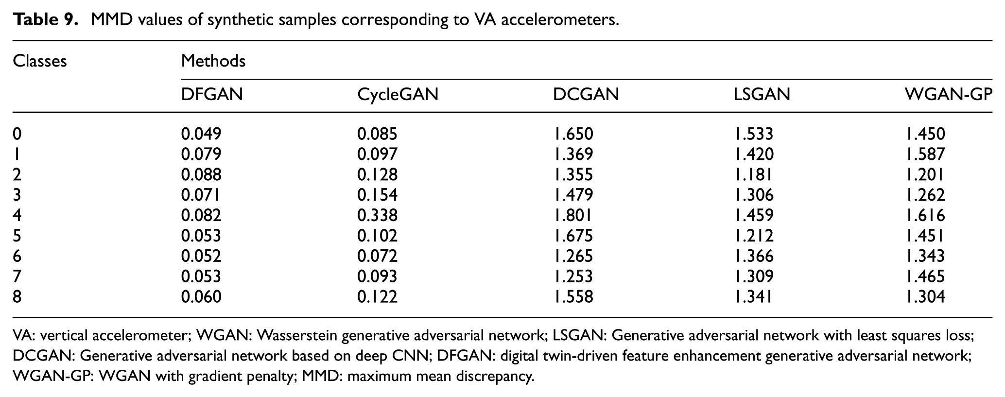
VA: vertical accelerometer; WGAN: Wasserstein generative adversarial network; LSGAN: Generative adversarial network with least squares loss; DCGAN: Generative adversarial network based on deep CNN; DFGAN: digital twin-driven feature enhancement generative adversarial network; WGAN-GP: WGAN with gradient penalty; MMD: maximum mean discrepancy.

Experimental results and discussion

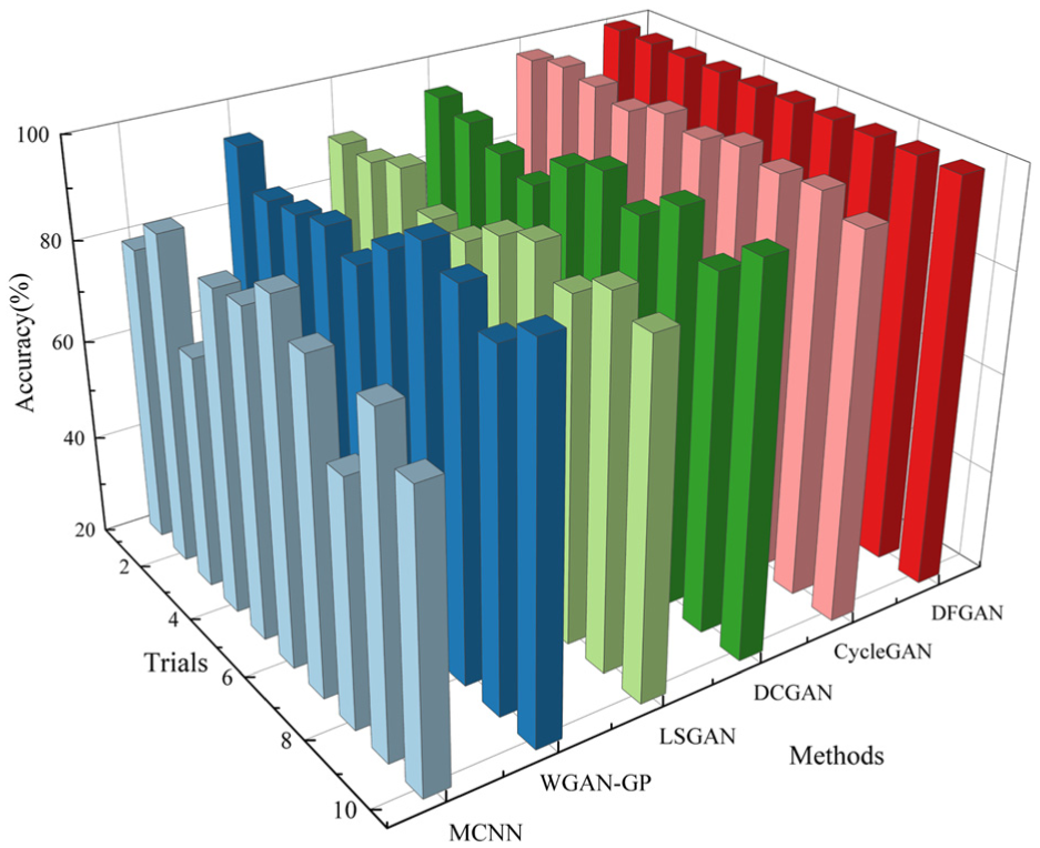
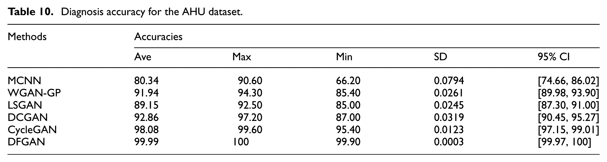
Using the imbalanced data from the VA and HA sensors, the diagnosis results obtained are displayed in Figure 17 and Table 10. MCNN, WGAN-GP, LSGAN, DCGAN, and CycleGAN achieved average accuracies of 80.34%, 91.94%, 89.15%, 92.86%, and 98.08%, respectively, all of which are lower than the average accuracy (99.99%) of DFGAN, demonstrating the superiority of the latter. With the assistance of DT, the diagnostic accuracy of DFGAN was improved by 36.72% on the AHU dataset compared to MCNN. This suggests that the fault information embedded in DT models based on real physical mechanisms can effectively enhance the performance of diagnostic models. In addition, after 10 trials, the SD of the experimental accuracies of MCNN, WGAN-GP, LSGAN, DCGAN, CycleGAN, and DFGAN was 0.0794, 0.0261, 0.0245, 0.0319, 0.0123, and 0.0003, respectively, indicating that DFGAN exhibited more stable diagnostic performance. The 95% CI for the diagnostic results of DFGAN on the AHU dataset is [99.97, 100], which is the narrowest and does not overlap with those of the comparison methods. In other words, the performance of DFGAN has excellent robustness.

Figure 17.

Diagnosis results for AHU dataset.

Table 10.

Diagnosis accuracy for the AHU dataset.

Methods	Accuracies
	Ave	Max	Min	SD	95% CI
MCNN	80.34	90.60	66.20	0.0794	[74.66, 86.02]
WGAN-GP	91.94	94.30	85.40	0.0261	[89.98, 93.90]
LSGAN	89.15	92.50	85.00	0.0245	[87.30, 91.00]
DCGAN	92.86	97.20	87.00	0.0319	[90.45, 95.27]
CycleGAN	98.08	99.60	95.40	0.0123	[97.15, 99.01]
DFGAN	99.99	100	99.90	0.0003	[99.97, 100]

As Figure 18(a) shows, the diagnostic accuracy for class 0 was only 27%, while that for class 7 was as low as 17%, the performance of MCNN was much lower than that of the other methods. As illustrated in Figures. 18(b) to (e), the diagnostic performance of WGAN-GP, LSGAN, DCGAN, and CycleGAN was directly affected by the poor quality of the synthetic samples that they generated. WGAN-GP has low diagnostic accuracy for test samples from class 1 and class 4, only 64% and 63%, respectively. LSGAN and DCGAN achieved diagnostic accuracy of 35% and 73% for class 0, and the corresponding values for class 8 were 66% and 78%, respectively. This implies that neither LSGAN nor DCGAN can accurately identify samples from classes 3 and 5. CycleGAN also struggled to accurately distinguish test samples from class 4 (78%). In contrast, Figure 18(f) demonstrates that DFGAN achieved the highest diagnostic accuracy across all fault conditions, demonstrating its superior generalization performance.

Figure 18.

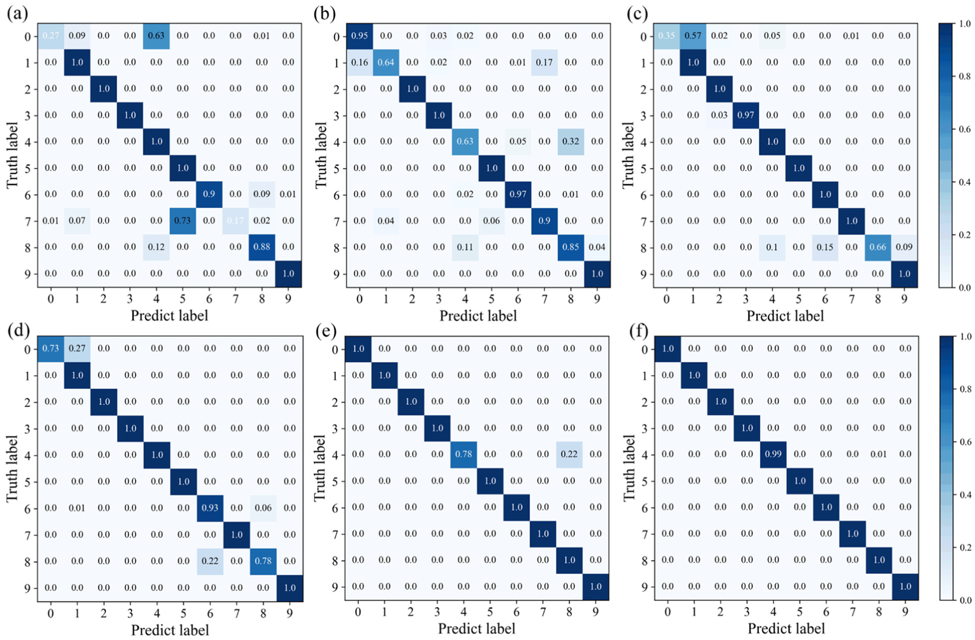
Confusion matrices for AHU dataset: (a) MCNN, (b) WGAN-GP, (c) LSGAN, (d) DCGAN, (e) CycleGAN, and (f) DFGAN.

Analysis of synthetic samples with different number

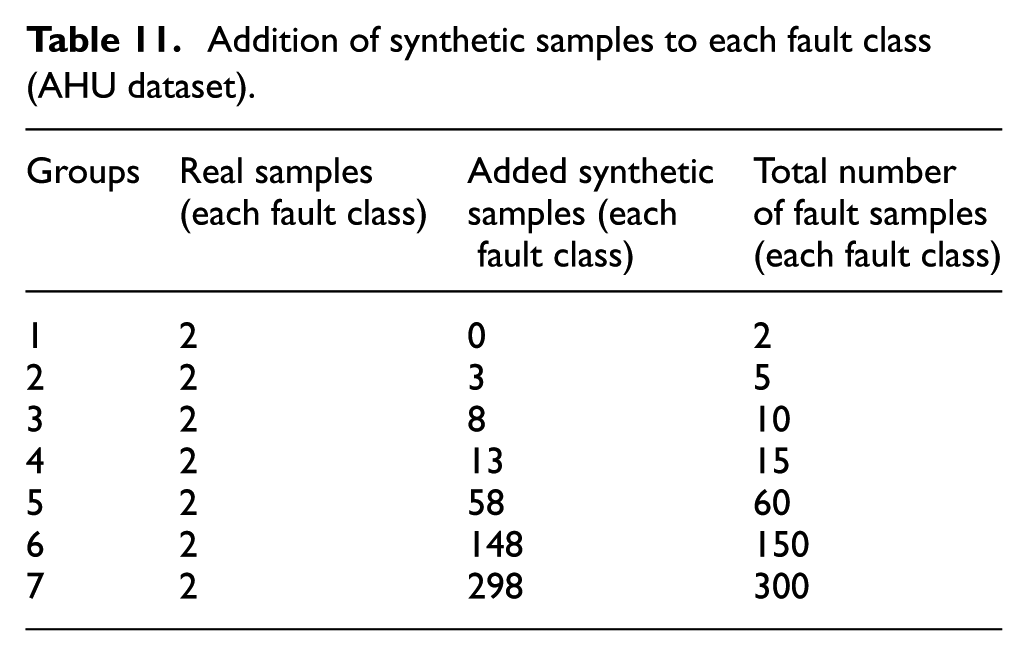
The insufficient samples of a minority class (Class 0–Class 9) are augmented through synthetic samples obtained by different methods, respectively, to investigate the effect of the number of samples on the classifier performance. The imbalanced data are gradually restored to the equilibrium state. As presented in Table 11, the number of synthetic samples added to each fault class is 3, 8, 13, 58, 148, and 298, respectively, and the classifier performance is tested by the augmented data with the same experimental setup as in Section “Experimental results and discussion.”

Table 11.

Addition of synthetic samples to each fault class (AHU dataset).

Groups	Real samples (each fault class)	Added synthetic samples (each fault class)	Total number of fault samples (each fault class)
1	2	0	2
2	2	3	5
3	2	8	10
4	2	13	15
5	2	58	60
6	2	148	150
7	2	298	300

The diagnostic results obtained by adding different numbers of synthetic samples are illustrated in Figure 19. Similar to the diagnostic results obtained on the CWRU dataset, the diagnostic accuracy corresponding to all the methods on the AHU dataset is improved as the number of synthetic samples increases. Compared to the comparison method, the diagnostic accuracies achieved by the proposed method with different numbers of synthetic samples are 95.96%, 96.70%, 99.41%, 99.85%, 99.98%, and 99.99%, respectively, which are all better than the corresponding values of the comparison method. After the total number of fault samples for each fault class reaches 15, the performance of the proposed method tends to stabilize, with diagnostic accuracies all over 99%. To sum up, even a small number of synthetic samples obtained with DFGAN can achieve good diagnostic accuracy, which proves the superiority of DFGAN.

Figure 19.

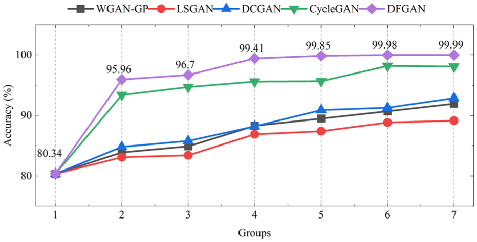
Diagnosis accuracy with different number of added fault samples in each fault class (AHU dataset).

Summary of diagnostic results on Case 1 and Case 2

The CWRU dataset and AHU dataset contain 10 types of fault data of SKF 6203 and NSK 6012 bearings, respectively, to verify the generalization ability of the DFGAN. Different from the CWRU dataset, the AHU dataset obtained the compound fault data of rollers and inner raceway through a self-built test bench. Compared to comparison methods, DFGAN achieved the lowest MMD between synthetic and measured samples across all fault classes on both datasets, demonstrating the effectiveness of synthetic samples generated by DFGAN. Using synthetic samples to augment imbalanced data, DFGAN exhibited superior performance on both the CWRU and AHU datasets. Moreover, it achieved diagnostic accuracies of 99.96% and 99.99%, respectively, significantly outperforming existing comparison methods. Additionally, the increase in the number of added synthetic samples contributes to the improved diagnostic performance. Diagnostic results indicate that the performance of DFGAN stabilizes on both datasets once the total number of samples for each fault class reaches 15.

Parameter analysis

The above results specify that DFGAN achieve the best diagnostic results on both CWRU and AHU datasets compared with the comparison method. However, the training parameters of DFGAN may affect its ability to synthesize fault sample generation. In this section, the merits of the proposed method are further verified from two perspectives: hyperparameter tuning and the number of measured fault samples for training.

Hyperparameter tuning

Analysis of learning rate lr

The learning rate (lr) is a critical hyperparameter that directly influences the final performance of DFGAN. While the models with large learning rates may skip the optimal solution, too small learning rates may not allow the model to converge quickly. With the purpose of determining the optimal learning rate of DFGAN, Adam is selected for model parameter optimization algorithms, and the cosine annealing algorithm is employed to update the lr. Meanwhile, the initial lr of DFGAN is set in the range of 5e−6 to 5e−3 to obtain synthetic samples and augment the dataset. The diagnostic results of the two datasets at different learning rates are illustrated in Figure 20(a).

Figure 20.

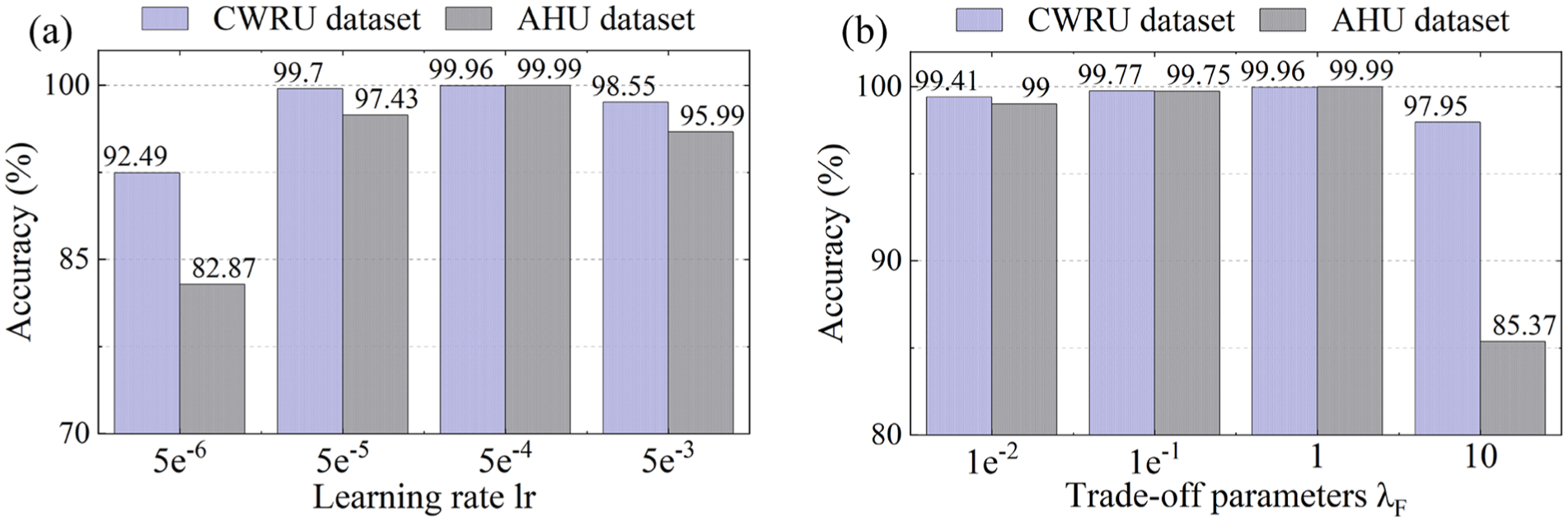
The diagnostic accuracy obtained by DFGAN of CWRU and AHU datasets with different hyperparameters: (a) learning rate lr, (b) trade-off parameter λ_F.

Figure 20(a) suggests that the imbalanced fault diagnosis accuracies on both CWRU and AHU datasets first increase and then decrease with the continuous increase in lr. Thus, both too large and too small learning rates can bring about a decrease in fault diagnosis accuracy. The effect of the learning rate lr on the diagnostic results of the AHU dataset is significantly larger than that of the CWRU dataset. When lr is equal to 5e–5, the proposed method achieves the highest diagnostic accuracy on both the CWRU and AHU datasets; therefore, it is reasonable to set the value of the learning rate lr to 5e−5.

Analysis of trade-off parameter λ_F

The spectral correlation loss L_F is adopted to achieve the alignment of the synthetic and measured sample distributions in the frequency domain. The trade-off parameter λ_F of the L_F impacts the DFGAN training. Therefore, the trade-off parameter λ_F is set to increase sequentially to find the optimal λ_F. In this section, the λ_F is set in the range of 1e−2 to 10 to obtain the synthetic samples and augment the dataset. The diagnostic results of the two datasets under different values of trade-off parameter λ_F are depicted in Figure 20(b).

As observed from Figure 20(b), the fault diagnosis accuracies on both the CWRU and AHU datasets first increase and then decrease as the λ_F continues to increase. When λ_F is equal to 1, the proposed method achieves the highest diagnostic accuracy on both CWRU and AHU datasets.

Number of measured fault samples for training

DFGAN can be applied to obtain synthetic fault samples and augment insufficient fault data. The augmented data can be adopted to adequately train the diagnostic model. All the above diagnostic results are obtained with DFGAN trained by two measured samples in each fault class (an imbalance ratio of 1:150). However, the number of measured fault samples also affects the performance of DFGAN. DFGAN is trained with 1, 2, and 4 measured fault samples in each fault class, which corresponds to imbalance ratios of 1:300, 1:150, and 1:75, respectively, to verify the robustness of the proposed method in extreme imbalance scenarios. The accuracies achieved by the diagnostic model on the two datasets with different numbers of real fault samples are detailed in Table 12.

Table 12.

Diagnostic accuracy with different numbers of measured fault samples.

No.	Imbalance ratios	Measured samples (each fault class)	Added synthetic (each fault class)	Accuracies of diagnosis (%)
				CWRU dataset	AHU dataset
1	1:300	1	299	99.49	99.73
2	1:150	2	298	99.96	99.99
3	1:75	4	296	100	100

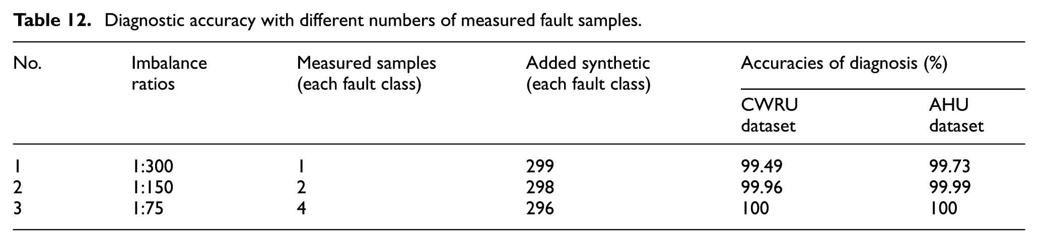
Table 1 reflects that, regarding the CWRU dataset, training DFGAN with 1, 2, and 4 measured samples in each fault state achieved diagnostic accuracies of 99.49%, 99.96%, and 100%, respectively, and the corresponding values for the AHU dataset were 99.73%, 99.99%, and 100%. The diagnostic accuracies of both CWRU and AHU datasets exceed 99% for different numbers of measured samples, verifying that the proposed DFGAN still maintains excellent performance in extreme imbalance scenarios. Furthermore, the diagnostic accuracies on both datasets surpass 99.9% when the number of measured samples for training the DFGAN exceeds 2, indicating the stable performance of the proposed method.

Ablation studies

DFGAN is multioptimized by the DT model, spectral correlation loss L_F, MCNN, and SEU-Net to obtain synthetic samples for use in augmenting the imbalanced data. In this section, four sets of imbalance fault diagnosis experiments are designed for ablation studies to demonstrate the necessity of the model design and evaluate the contribution of each part, so as to improve the model performance:

DFGAN without SEU-Net [M1]: ResNet⁵⁴ is used instead of SEU-Net as the structure of the DFGAN generator to investigate the impact of SEU-Net with multiple feature fusion layers on the model performance.

DFGAN without L_F [M2]: Spectral correlation loss L_F is removed from the loss function of DFGAN, and the alignment of the distribution of synthetic fault samples with measured fault samples in the frequency domain is ignored.

DFGAN without MCNN [M3]: A traditional CNN is employed to construct the classifier only through the data from a single sensor. Concerning the CWRU dataset, the data from FE sensors are selected for analysis. Regarding the AHU dataset, the data from the VA accelerometers dataset are selected for analysis.

DFGAN [M4]: In a control experiment, all parts are used to optimize DFGAN.

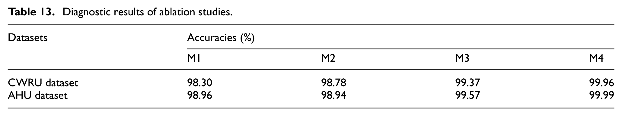
The setup of each experiment is the same as in Sections “Case1: CRUW dataset” and “Case2: Self-built dataset (AHU dataset), and only two measured samples are adopted to train the DFGAN for each fault class. All experiments are repeated 10 trials to minimize the error. The corresponding diagnostic results on the CWRU and AHU datasets are summarized in Table 13.

Table 13.

Diagnostic results of ablation studies.

Datasets	Accuracies (%)
	M1	M2	M3	M4
CWRU dataset	98.30	98.78	99.37	99.96
AHU dataset	98.96	98.94	99.57	99.99

Effectiveness of SEU-Net

In this section, the effectiveness of SEU-Net on the diagnostic model is investigated. The DFGAN without SEU-Net is compared with the DFGAN to evaluate the contribution of SEU-Net. The fault diagnosis results are summarized in Table 13. Compared with DFGAN without SEU-Net, the DFGAN achieves higher average accuracies, with 1.66% and 1.03% enhancements on the CWRU and AHU datasets, respectively. This enhancement is attributed to the effective extraction and deep fusion of fault information in the simulated samples by SEU-Net. Moreover, the simulated fault information is fully retained in the synthetic samples.

Contribution of spectral correlation loss L_F

DFGAN without L_F is compared with DFGAN to assess the contribution of the L_F, with the fault diagnosis results listed in Table 13. Specifically, the diagnosis accuracy of DFGAN on the CWRU and AHU datasets is improved by 1.18% and 1.05%, respectively, with the assistance of L_F. This is because the DFGAN training dynamics are guided by L_F, which improves the alignment of the synthetic samples with the measured samples in the frequency-domain distribution.

Effects of MCNN

In this section, the effect of the MCMM part is evaluated by comparing the DFGAN with the DFGAN without MCNN. The fault diagnosis results are summarized in Table 13, suggesting that DFGAN achieves a higher average accuracy compared to DFGAN without MCNN, with an enhancement of 0.59% and 0.42% on the CWRU and AHU datasets, respectively. This enhancement stems from the effective multisensor feature information extracted by branch CNNs in MCNN. The effective utilization of multisensor data improves the performance of learning fault feature representation.

Conclusion

To enhance the diagnostic accuracy of rolling bearings under imbalanced data, a DT-driven fault diagnosis method is proposed in this article. To generate simulated signals that obtain the dynamic response features of the system, a generic high-fidelity DT model with multiple DOFs is established using the lumped parameter method, employing fault and structure parameters as inputs. DFGAN is introduced to transform simulated fault samples from the DT model into synthetic samples with a data distribution similar to that of measured samples. The DFGAN generator is reconstructed with feature fusion layers, which extract and deeply fuses fault features from simulated samples. A spectral correlation loss based on the Pearson’s correlation of the spectra is designed, which reduces the discrepancy between synthetic and measured samples in the frequency domain. Subsequently, synthetic samples of the measured fault signals are employed to augment the imbalanced multisensor data, achieving imbalanced fault diagnosis of bearings.

The results of the quantitative analysis of the synthetic samples reveal that the proposed DFGAN obtained the lowest value of MMD between the synthetic and the measured samples compared to the existing advanced methods. Thus, the synthetic samples obtained by the proposed method exhibited superior quality compared to those obtained by existing advanced methods. Given two measured samples in each fault class, the proposed method achieved 99.96% and 99.99% diagnostic accuracies on the datasets of CWRU and AHU, respectively. The experimental results verified the superiority of the proposed method, which can significantly improve diagnostic accuracy and provide superior performance in imbalanced fault diagnosis for bearing systems. Furthermore, the results of ablation studies unveil that all parts of DFGAN can improve the diagnostic performance under imbalanced multisensor data, specifying the effectiveness of the model design. However, the simulation accuracy of vibration signals must be improved. In addition, the performance of GAN-based sample generation methods is low when the number of samples is insufficient, resulting in large discrepancies between generated synthetic samples and measured samples. Addressing these challenges will be a key focus in future research.

Footnotes

ORCID iD

Zhongding Fan

Funding

The authors disclosed receipt of the following financial support for the research, authorship, and/or publication of this article: This work was supported by the Anhui Province Science and Technology Tackling Key Problems Project (No. 202423i08050021), Anhui Province Key Research and Development Plan (No. 202304a05020058), Anhui Province Natural Science Foundation excellent youth project (No. 2408085Y029), National Natural Science Foundation of China (No. 52575087).

Declaration of conflicting interests

The authors declared no potential conflicts of interest with respect to the research, authorship, and/or publication of this article.

References

Matania

Dattner

Bortman

, et al. A systematic literature review of deep learning for vibration-based fault diagnosis of critical rotating machinery: limitations and challenges. J Sound Vib 2024; 590: 118562.

Tang

Yan

, et al. Deep transfer learning strategy in intelligent fault diagnosis of rotating machinery. Eng Appl Artif Intell 2024; 134: 108678.

Chen

Zhang

Gao

Bearing fault diagnosis base on multi-scale CNN and LSTM model. J Intell Manuf 2021; 32: 971–987.

Wang

Che

Semisupervised fault diagnosis of aeroengine based on denoising autoencoder and deep belief network. Aircr Eng Aerosp Technol 2022; 94: 1772–1779.

Ince

Kiranyaz

Eren

, et al. Real-time motor fault detection by 1-D convolutional neural networks. IEEE Trans Ind Electron 2016; 63: 7067–7075.

Tamilselvan

Wang

Failure diagnosis using deep belief learning based health state classification. Reliab Eng Syst Saf 2013; 115: 124–135.

Wang

An intelligent fault diagnosis model based on deep neural network for few-shot fault diagnosis. Neurocomputing 2021; 456: 550–562.

Liu

Zhang

Tan

, et al. Multi-scale quaternion CNN and BiGRU with cross self-attention feature fusion for fault diagnosis of bearing. Meas Sci Technol 2024; 35: 086138.

Liu

Liang

Guo

, et al. Fault diagnosis of rolling bearings under varying speeds based on gray level co-occurrence matrix and DCCNN. Measurement 2024; 235: 114955.

10.

Liang

Deng

Yuan

, et al. A deep capsule neural network with data augmentation generative adversarial networks for single and simultaneous fault diagnosis of wind turbine gearbox. ISA Trans 2023; 135: 462–475.

11.

Zhang

Liu

Zhang

, et al. Self-supervised graph feature enhancement and scale attention for mechanical signal node-level representation and diagnosis. Adv Eng Inform 2025; 65: 103197.

12.

Zhang

Kang

, et al. Fault diagnosis of rotating machinery based on dual convolutional-capsule network (DC-CN). Measurement 2021; 187: 110258.

13.

Feng

, et al. Domain constrained cascadic multireceptive learning networks for machine health monitoring in complex manufacturing systems. J Manuf Syst 2025; 80: 563–577.

14.

Zhong

Lin

Huang

, et al. Multi-adversarial subdomain adaptation network for unsupervised fault diagnosis. Mech Syst Signal Process 2025; 236: 113031.

15.

Zhang

, et al. Multi-scale group Mamba network with structural attention for rotating machinery fault diagnosis using multisensor data. Adv Eng Inform 2025; 67: 103521.

16.

Yan

Zhang

Liu

Multi-branch convolutional neural network with generalized shaft orbit for fault diagnosis of active magnetic bearing-rotor system. Measurement 2021; 171: 108778.

17.

Wang

Mao

Bearing fault diagnosis based on vibro-acoustic data fusion and 1D-CNN network. Measurement 2021; 173: 108518.

18.

Shen

Song

, et al. Multi-sensor and multi-level information fusion model for compressor blade crack detection. Measurement 2023; 222: 113622.

19.

Zhang

Jiao

, et al. Intelligent fault diagnosis of bearings driven by double-level data fusion based on multichannel sample fusion and feature fusion under time-varying speed conditions. Reliab Eng Syst Saf 2024; 251: 110362.

20.

Zhang

Wang

Blockchain-based decentralized federated transfer learning methodology for collaborative machinery fault diagnosis. Reliab Eng Syst Saf 2023; 229: 108885.

21.

Pan

Chen

Zhang

, et al. Generative adversarial network in mechanical fault diagnosis under small sample: a systematic review on applications and future perspectives. ISA Trans 2022; 128: 1–10.

22.

Zhang

Chen

, et al. Intelligent fault diagnosis of machines with small & imbalanced data: a state-of-the-art review and possible extensions. ISA Trans 2022; 119: 152–171.

23.

Liu

Jiang

, et al. Rolling bearing fault diagnosis using variational autoencoding generative adversarial networks with deep regret analysis. Measurement 2021; 168: 108371.

24.

Liang

Deng

, et al. Intelligent fault diagnosis of rotating machinery via wavelet transform, generative adversarial nets and convolutional neural network. Measurement 2020; 159: 107768.

25.

Pan

Chen

Xie

, et al. Deep feature generating network: a new method for intelligent fault detection of mechanical systems under class imbalance. IEEE Trans Ind Inform 2021; 17: 6282–6293.

26.

Zhang

, et al. Rotating machinery fault detection and diagnosis based on deep domain adaptation: a survey. Chin J Aeronaut 2023; 36: 45–74.

27.

Zhong

Shao

, et al. Multi-mode data augmentation and fault diagnosis of rotating machinery using modified ACGAN designed with new framework. Adv Eng Inform 2022; 52: 101552.

28.

Meng

Kong

, et al. Generative adversarial networks for gearbox of wind turbine with unbalanced data sets in fault diagnosis. IEEE Sens J 2022; 22: 13285–13298.

29.

Guo

, et al. CSWGAN-GP: a new method for bearing fault diagnosis under imbalanced condition. Measurement 2023; 217: 113014.

30.

Guo

Wang

Sun

, et al. Imbalanced data fault diagnosis method for nuclear power plants based on convolutional variational autoencoding Wasserstein generative adversarial network and random forest. Nucl Eng Technol 2024; 56: 5055-5067.

31.

Liu

, et al. A multi-domain adversarial transfer network for cross domain fault diagnosis under imbalanced data. Eng Appl Artif Intell 2024; 136: 108948.

32.

Tang

Chu

Generative adversarial networks for prognostic and health management of industrial systems: a review. Expert Syst Appl 2024; 253: 124341.

33.

Bisanti

Mainetti

Montanaro

, et al. Digital twins for aircraft maintenance and operation: a systematic literature review and an IoT-enabled modular architecture. Internet Things 2023; 24: 100991.

34.

Xia

Huang

Tao

, et al. A digital twin-enhanced semi-supervised framework for motor fault diagnosis based on phase-contrastive current dot pattern. Reliab Eng Syst Saf 2023; 235: 109256.

35.

Zhou

Xiong

, et al. Simulation data-driven attention fusion network with multi-similarity metric: a single-domain generalization diagnostic method for tie rod bolt loosening of a rod-fastening rotor system. Measurement 2025; 240: 115565.

36.

Kong

Wang

, et al. Intelligent fault diagnosis of bearings under small samples: A mechanism-data fusion approach. Eng Appl Artif Intell 2023; 126: 107063.

37.

Jiang

, et al. Digital twin-driven focal modulation-based convolutional network for intelligent fault diagnosis. Reliab Eng Syst Saf 2023; 240: 109590.

38.

Yan

Zhong

Shao

, et al. Digital twin-assisted imbalanced fault diagnosis framework using subdomain adaptive mechanism and margin-aware regularization. Reliab Eng Syst Saf 2023; 239: 109522.

39.

Zhang

Ren

, et al. Digital twin-driven partial domain adaptation network for intelligent fault diagnosis of rolling bearing. Reliab Eng Syst Saf 2023; 234: 109186.

40.

Zhao

Zhang

Fan

, et al. Research on rolling bearing virtual-real fusion life prediction with digital twin. Mech Syst Signal Process 2023; 198: 110434.

41.

Xia

Huang

Chen

, et al. A novel digital twin-driven approach based on physical-virtual data fusion for gearbox fault diagnosis. Reliab Eng Syst Saf 2023; 240: 109542.

42.

Liu

Xiang

, et al. A transfer learning strategy based on numerical simulation driving 1D Cycle-GAN for bearing fault diagnosis. Inf Sci 2023; 642: 119175.

43.

Qin

Liu

Mao

Faulty rolling bearing digital twin model and its application in fault diagnosis with imbalanced samples. Adv Eng Inform 2024; 61: 102513.

44.

Feng

Wang

, et al. Digital twin enabled domain adversarial graph networks for bearing fault diagnosis. IEEE Trans Ind Cyber Phys Syst 2023; 1: 1–10.

45.

Liu

Shao

Dynamic modeling for rigid rotor bearing systems with a localized defect considering additional deformations at the sharp edges. J Sound Vib 2017; 398: 84–102.

46.

Gupta

PK.

Dynamic loads and cage wear in high-speed rolling bearings. Wear 1991; 147: 119–134.

47.

Qin

, et al. Multiple-degree-of-freedom dynamic model of rolling bearing with a localized surface defect. Mech Mach Theory 2020; 154: 104047.

48.

Tiwari

Gupta

Prakash

Dynamic response of an unbalanced rotor supported on ball bearings. J Sound Vib 2000; 238: 757–779.

49.

Cao

Jing

, et al. Vibration mechanism analysis for cylindrical roller bearings with single/multi defects and compound faults. Mech Syst Signal Process 2020; 144: 106903.

50.

Feng

Chen

Zhang

, et al. Semi-supervised meta-learning networks with squeeze-and-excitation attention for few-shot fault diagnosis. ISA Trans 2022; 120: 383–401.

51.

Wang

Zhang

Chen

, et al. Enhanced generative adversarial network for extremely imbalanced fault diagnosis of rotating machine. Measurement 2021; 180: 109467.

52.

Huo

Gan

Jiang

Multi-exposure high dynamic range imaging based on LSGAN. Displays 2024; 83: 102707.

53.

Wei

Liu

Yue

, et al. A multi-sensor signals denoising framework for tool state monitoring based on UKF-CycleGAN. Mech Syst Signal Process 2023; 200: 110420.

54.

Zhao

Huang

Transfer learning method for rolling bearing fault diagnosis under different working conditions based on CycleGAN. Meas Sci Technol 2021; 33: 025003.

Digital twin-driven feature enhancement generative adversarial network for rolling bearings fault diagnosis

Abstract

Keywords

Introduction

The DT model of bearings

Development of DT model

Verification of simulated signals

Framework for imbalanced fault diagnosis

Principle of DFGAN

SEU-Nets for generators

Patch-GAN for discriminators

The loss function with spectral correlation loss of the DFGAN

MCNN for fault diagnosis

Experiment and analysis

Training details

Methods for comparison

Case1: Case Western Reserve University (CWRU) dataset

Description and processing of dataset

Evaluation of synthetic samples

Experimental results and discussion

Analysis of synthetic samples with different number

Case2: Self-built (AHU) dataset

Description and processing of dataset

Evaluation of synthetic samples

Experimental results and discussion

Analysis of synthetic samples with different number

Summary of diagnostic results on Case 1 and Case 2

Parameter analysis

Hyperparameter tuning

Analysis of learning rate lr

Analysis of trade-off parameter λF

Number of measured fault samples for training

Ablation studies

Effectiveness of SEU-Net

Contribution of spectral correlation loss LF

Effects of MCNN

Conclusion

Footnotes

ORCID iD

Funding

Declaration of conflicting interests

References

Analysis of trade-off parameter λ_F

Contribution of spectral correlation loss L_F