
Abstract
Expanding artificial intelligence methods to the domain of structural damage detection can effectively enhance the detection accuracy and efficiency. Models like convolutional neural networks can effectively capture significant features related to structural damage. However, due to the receptive field constraints, it is difficult to fully capture the global characteristics of the data. In addition, considering structural damage identification and damage location as a single task will lead to a large number of label classifications, thereby increasing the requirements for model complexity and training data quality. To address these issues, a multiscale fusion-based multitask Transformer (MFMTT) model based on a multivariate time-series Transformer is proposed in this paper. The encoder structure of Transformer is employed to extract the global features of sequence data, and the structural damage detection task is divided into two subtasks, each of which has a lower number of categories than the single-task one. The proposed MFMTT model is validated using a numerical simulation dataset of a simply supported beam and the International Association for Structural Control – American Society of Civil Engineers (IASC-ASCE) phase II benchmark experimental dataset, ensuring reproducibility across both synthetic and real-world scenarios. The experimental results demonstrate that the MFMTT model achieves accurate identification of structural damage states across single-damage scenarios, multidamage conditions, and benchmark experimental setups, with damage detection accuracy exceeding 99%.
Introduction
Although most structures are designed for a long service life, damage to critical components can significantly weaken their performance, potentially leading to catastrophic consequences. Assessing the health of a structure allows for early detection of potential safety hazards, which serves as a basis to formulate maintenance plans. However, it is a significant challenge to evaluate the structure’s health status accurately and reliably under normal use conditions. Structural damage detection (SDD) is a crucial aspect in solving this challenge.1–3
The dynamic response of a structure will be affected accordingly when structural damage occurs, and this change can reflect the structural damage state. Therefore, the vibration-based damage detection methods are extensively utilized in structural health monitoring (SHM). 4 There are two main classifications of these methods: model-based methods and data-driven methods. 2 Damage detection using the model-based methods is achieved through a comparison between the response of the actual structure and that of the baseline finite-element model.5–9 However, these models necessitate the development of precise finite-element models, a process that is often tedious and may not effectively reflect the actual response of the structure to complex environmental influences. 10 In contrast, data-driven methods depend on field measurement data solely. 11 They employ data-mining techniques to extract structural damage information from time-series data measured by sensors. 12 Ahmadi et al. 13 and Gharehbaghi et al. 14 achieved the detection of structural damage by analyzing the acceleration response of the structure. Expanding artificial intelligence methods into the domain of SDD has emerged as a current research hot topic. Machine learning (ML) algorithms (including Bayes,15–18 decision trees, 19 neural networks,20–23 and deep learning (DL) models24,25) offer a wider range of options for data-driven methods. These methods require a training process that utilizes structural response data to learn the internal parameters of the model, enabling rapid prediction of structural damage. 26
Currently, a variety of neural-network-based methods have been proposed for SDD. Among these, convolutional neural networks (CNNs) have demonstrated significant potential. Lin et al. 27 proposed a supervised CNN model and achieved the effective identification of structural damage by using labeled acceleration data. Li et al. 28 proposed a damage identification method based on strain modal difference by utilizing the inverse finite-element method, in which strain modal difference is employed as the input to CNN to achieve structural damage location and quantification. Abdeljaber et al. 29 employed a one-dimensional CNN to process SHM data for structural damage classification.
However, CNNs face inherent limitations in SDD: their reliance on fixed-length convolutional kernels and uniform weight assignment across data segments restricts the model’s receptive field size and global sensitivity, potentially leading to unstable or inaccurate damage identification results. SHM systems predominantly generate long-duration time-series data. Effective damage state identification in such scenarios necessitates methods capable of efficiently capturing long-range temporal dependencies. The Transformer architecture addresses these limitations through its self-attention mechanism. Originally proposed by Vaswani et al., 30 Transformers explicitly model long-range dependencies in sequential data by dynamically weighting inter-element relationships via attention mechanisms. Beyond its seminal success in natural language processing, 31 Transformers have demonstrated cross-domain adaptability in audio processing, computer vision, and increasingly in multivariate time-series analysis, which is a nascent yet critical frontier for SHM applications. Zerveas et al. 32 proposed a Transformer-based framework to process and classify multivariate time-series data. Triviño et al. 33 utilized this framework to achieve the damage detection and localization of offshore wind turbines.
In SDD, most of the methods using supervised learning techniques consider structural damage severity identification and damage location as a single task, combining the damage degree with the damage location and setting classification labels accordingly. 34 However, the increase in the number of classifications also leads to higher demands for training data and model complexity in supervised learning methods. In contrast, dividing the damage detection task into two subtasks, namely, damage identification and damage location, can significantly reduce the number of classification categories for each task. When multiple tasks are similar to each other, and the training data for each task are limited, adopting a multitask learning (MTL) framework provides an effective means of jointly addressing damage severity identification and damage scenario classification within a unified model. Designing deep architectures for joint tasks has achieved some successes in some visual tasks.35–37 The application of MTL methods has recently expanded into the domain of SDD.38,39 Gao et al. 40 established a vision-based multitask SDD framework. Kord et al. 41 constructed an SDD framework by combining MTL and a three-dimensional CNN. Liu et al. 42 proposed a hierarchical multitask framework that utilizes labeled data from the source domain and data from the target domain for SDD. These studies implemented damage identification and localization within a shared multitask model. However, they retained data samples from healthy structures during localization, which may introduce redundant parameters and increase computational complexity.
To address the above challenges, this study proposes a multiscale fusion-based multitask Transformer (MFMTT) framework for vibration-based SDD. In contrast to existing Transformer-based SDD approaches that predominantly address single-task damage classification or adopt parallel MTL schemes,35,40–42 the MFMTT explicitly accounts for the inherent dependency between damage degree detection and damage location. In the proposed formulation, task 1 performs cross-entropy-based damage severity identification with an additional binary damage-existence decision, whereas task 2 performs cross-entropy-based damage localization over a predefined set of candidate locations.
In contrast to existing Transformer-based SDD models that primarily address single tasks, as well as parallel multitask frameworks that treat damage detection and damage location independently, the MFMTT explicitly models these tasks as sequentially dependent and embeds the practical SDD decision logic into the network architecture. A key contribution of the MFMTT is a prediction-driven sequential filtering mechanism, in which the output of damage detection is used to condition subsequent damage localization. By excluding healthy samples before scenario classification-related processing, this mechanism reduces redundant computation and effectively mitigates the severe class imbalance inherent in vibration-based SDD, without introducing additional supervision or annotations. In addition, the MFMTT employs an integrated global–local feature representation that combines Transformer-based long-range temporal modeling with multiscale dilated convolutional feature fusion, enabling the framework to capture both global structural response patterns and localized damage-sensitive features, and thereby addressing limitations observed in CNN-only or Transformer-only SDD approaches.
The organization of this paper is outlined as follows: the first section: Introduction; the second section: The proposed model; the third section: Numerical verification; the fourth section: Experimental verification; the fifth section: Conclusion.
The proposed model
In this section, the proposed MFMTT for SDD is introduced, as shown in Figure 1. The main components of the MFMTT include a feature extractor and a classifier. Once the data preprocessing is complete, it is passed to the feature extractor. Subsequently, the data processed by the feature extractor are first flattened before being finally input into the classifier to generate the final damage identification results.
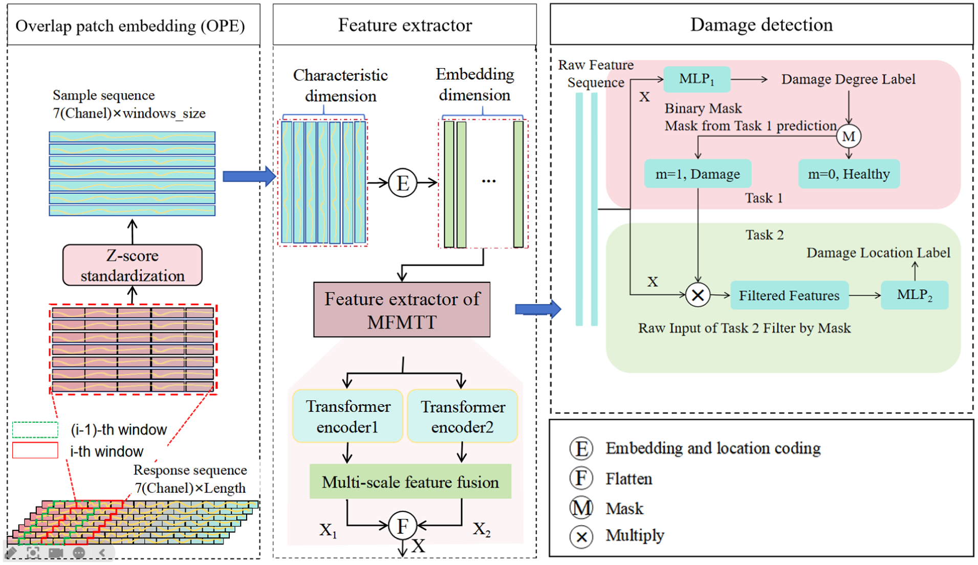
Flowchart of the proposed MFMTT model. MFMTT: multiscale fusion-based multitask Transformer.
Overlapping patch embedding technique
Images are typically divided into nonoverlapping patches for processing by traditional image processing or feature extraction methods, which may lead to a loss of local continuity. In contrast, the overlapping patch embedding (OPE) technique, which allows for overlapping areas between patches, enables better capture of local correlations. In this study, the structural acceleration response data are presented as long sequences, and directly inputting this data into the model significantly increases computational complexity and resource demands. Therefore, this study employs the OPE technique to divide the original acceleration data into shorter patches for processing. Specifically, the collected data are segmented into sample data with a length equal to the window size using overlapping sliding time windows. 43 Compared to the convolution-based overlapping patch division method, the sliding window calculation used in this study is simpler and more efficient. Additionally, the data within each window consist of segments of the original data, resulting in processing outcomes with stronger interpretability.
Feature extractor for the MFMTT
In the MFMTT, the feature extractor consists of two transformer encoders and a multiscale feature fusion module, which is shared by two tasks, that is, damage identification and damage location. The two tasks share a single feature extractor, allowing them to share the same learning feature representation. By sharing features, fewer parameters will be needed, and the network will be able to generalize over a wider range of samples. The Transformer encoder has remarkable capacity to capture long-distance dependencies in sequence data and model remote interactions.44–47 The two Transformer encoders differ in feature dimension and number of encoding layers. Each encoder structure corresponds to an independent classifier, with the classification processes for the two tasks conducted separately. This eliminates the need for feature dimension alignment. The feature fusion module is composed of dilated convolutional layers with varying dilation rates, which are employed to extract multiscale local features from the response data. These features are subsequently fused through an integration process. The module leverages dilated convolutions with exponentially increasing dilation rates (e.g., 1, 2, 4, 8) to progressively expand receptive fields while maintaining computational efficiency.
For vibration-based SDD tasks, structural responses are commonly utilized as training data for models. In this study, multivariate time-series data, which are composed of acceleration responses from different positions of structures under various damage conditions, are employed. The MFMTT can fuse the information of each feature in a multivariate time series, combining local features with global features, so as to completely extract the information in the data.
Classifier and sequential filtering mechanism for the MFMTT
The classifier of the MFMTT consists of two lightweight multilayer perceptrons (MLPs) and a sequential filtering layer, corresponding to damage severity identification (task 1) and damage scenario classification (task 2), respectively. After feature extraction, the shared feature representation is flattened and first fed into the task 1 classifier to estimate the damage state of each sample. Task 2 is formulated as a damage location classification problem over a finite set of predefined damage scenarios, rather than a continuous localization task.
Under this formulation, the model assumes that damage patterns encountered during inference are consistent with those observed during training. If damage configurations deviate from the predefined scenarios or fall outside the training distribution, the performance of the MFMTT may degrade. This behavior is not specific to the proposed framework, but is a common limitation of supervised, classification-based SDD methods that rely on discretized damage scenarios and labeled data. Similar generalization issues have been reported in previous data-driven SDD studies, where model performance depends strongly on the representativeness of the training set. Accordingly, the MFMTT is not intended to address this inherent constraint, but to provide a coherent multitask formulation that improves damage identification and scenario classification within the standard supervised learning setting.
Let
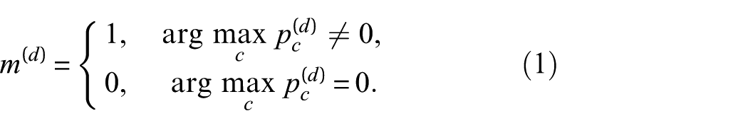
This mask determines whether a given sample is forwarded to task 2. Samples classified as healthy (m = 0) are excluded from the damage scenario classification task and are used only for damage severity identification.
Importantly, the same prediction-driven mask generation strategy is adopted during both training and inference. The mask is always derived from task 1 predictions rather than ground-truth labels, ensuring full consistency between training and testing pipelines and avoiding teacher-forcing-induced discrepancies. During training, the loss of task 2 is computed only for samples with m = 1, such that the scenario classification loss can be expressed as
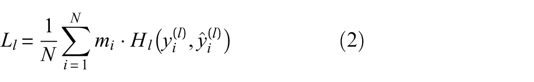
where
Although task 2 depends on task 1 through the filtering mechanism, error propagation is limited in practice due to the high reliability of damage detection. In all numerical and experimental benchmarks considered in this study, task 1 maintains an accuracy of nearly 95% or higher, resulting in a negligible proportion of damaged samples being incorrectly filtered. The primary purpose of this sequential filtering mechanism is therefore not to enhance robustness under severe misclassification scenarios, but to reduce redundant computation and mitigate class imbalance in damage scenario classification by removing healthy samples that are irrelevant to task 2.
Activation function
The activation function holds an important position in the neural network. Since it introduces nonlinear factors into the neural network model, it significantly enhances the model’s expressive ability and enables the neural network to fit a wide variety of complex nonlinear functions. Among the activation functions commonly used are the Sigmoid function, Rectified Linear Unit (ReLU), Exponential Linear Unit (ELU), 48 Gaussian Error Linear Unit (GELU), 49 and so on, and their function images are shown in Figure 2. Although the ReLU function is simple to compute and has a high computational efficiency, it is prone to leading to the disappearance of the gradient and the death of the neurons. The ELU function has a gradient that will gradually decrease in the negative input interval, which may lead to the disappearance of the gradient. It is noteworthy that the GELU function excels at approximating complex functions. Thus, this function is chosen for activation in this study. The mathematical expression of the activation function in this paper is:

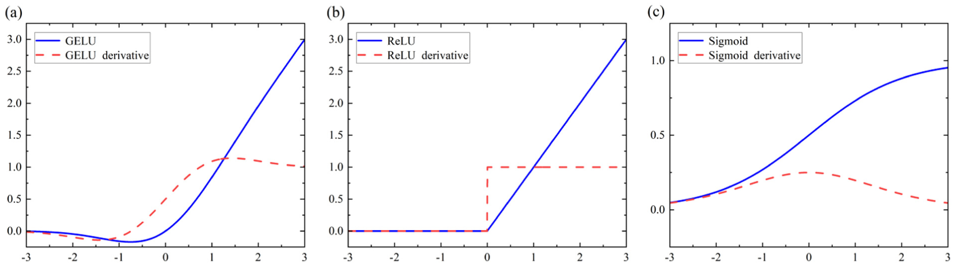
Activation functions and their derivatives: (a) GELU, (b) ReLU, and (c) Sigmoid.
The Gaussian distribution function
Global loss function
In this study, we focus on two classification tasks: damage degree identification and damage scenario classification. For both tasks, we utilize the cross-entropy loss function, which helps the model learn the discrepancies between the true distributions and the predicted distributions during training. The loss function for the damage degree identification task is:

In this equation, p(ydi) is the true probability distribution of the ith damage degree. q(ydi) denotes the predicted probability distribution of the ith damage degree. For the damage scenario classification task, the loss function is similarly defined:
where

Following the formulation of the global loss in Equation (4), the weighting coefficients ζ d and ζ1 are introduced to balance the relative contributions of damage severity identification (task 1) and damage scenario classification (task 2) during joint optimization. In the proposed MFMTT framework, the two tasks differ in both classification granularity and learning difficulty. Task 1 involves a larger number of classes and serves as a prerequisite for subsequent processing, whereas task 2 is only activated for samples predicted as damaged. In this study, the values of ζ d = 0.6 and ζ1 = 0.4 are used. These values were determined through empirical tuning based on validation performance, where different weight combinations were evaluated to balance convergence stability and overall accuracy across both tasks. The selected configuration consistently yielded robust performance on both the numerical beam model and the benchmark experimental dataset, and was therefore adopted for all subsequent experiments.
Implementation details of the MFMTT
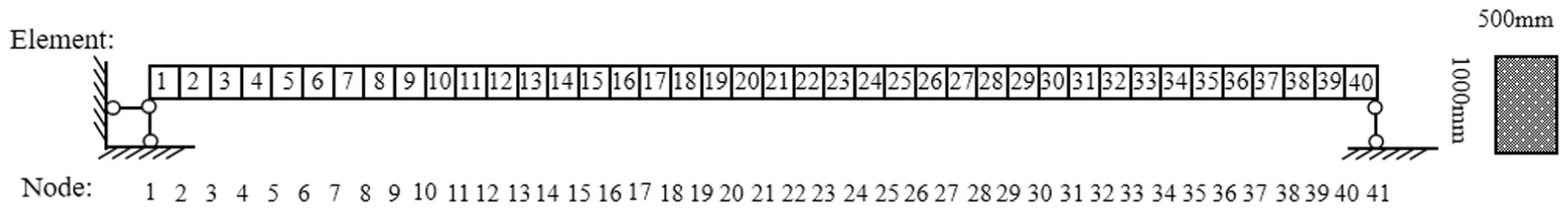
To ensure model reproducibility, this section provides a focused analysis of the key implementation details of the MFMTT. For clarity, the main architectural configurations, data preprocessing settings, and training hyperparameters of the proposed MFMTT are summarized in Table 1. The table provides an overview of the Transformer encoder, multiscale fusion module, classifier structure, as well as the associated preprocessing and training settings, and is intended to facilitate implementation and comparison.
Key structures and hyperparameters of the MFMTT.
MFMTT: multiscale fusion-based multitask Transformer; OPE: overlapping patch embedding.
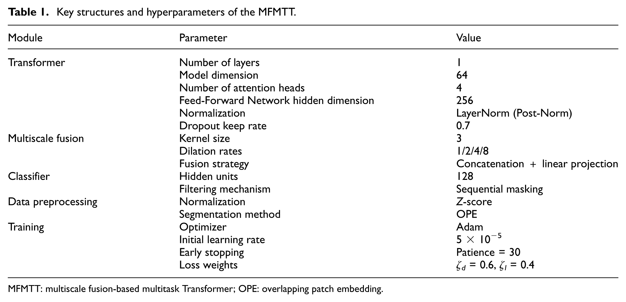
SDD based on the MFMTT
The workflow of the MFMTT model for SDD is illustrated in Figure 3. The labeled raw data are standardized and then divided into three subsets: a training set, a validation set, and a test set. The training and validation sets are used to train the model, while the test set is used to assess the model’s ability to recognize unknown data and predict the structural damage state from the structural response acceleration data. Subsequently, in these datasets, long sequence data are divided into shorter sample sequences.
Workflow of structural damage detection.
In vibration-based SDD, CNNs have been widely applied but show limitations in handling long time-series data and complex spatial features due to their fixed convolution kernels and limited receptive fields. To address this, the proposed MFMTT model adopts OPE with multiscale feature fusion, enabling efficient long-sequence processing while reducing computational cost. Its parameters mainly consist of three core modules. The transformer encoder, consisting of a single layer, incorporates multihead self-attention and a feedforward network, with a model dimension of 64. The multiscale feature fusion includes four dilated convolution layers with different dilation rates (convolution kernel size 3). The classifier incorporates two lightweight MLPs, reducing dependence on the encoder.
Numerical verification
In this section, the validation of the proposed MFMTT model is performed using a numerical simulation dataset of a simply supported beam. The acceleration responses of the beam across various damage scenarios are simulated. Then, the acceleration data are preprocessed, which include standardizing the data, organizing the dataset, and dividing the data by the OPE technique. The effect of model hyperparameters on performance is also investigated. Finally, the effectiveness of the proposed method for SDD is validated by the simply supported beam damage detection results.
Numerical simulation
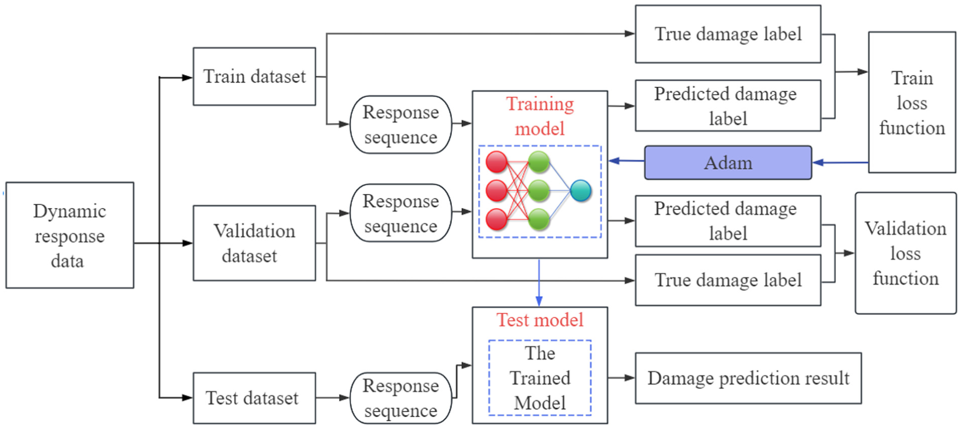
The dynamic response of a simply supported RC beam with a span of 20 m is calculated using OpenSees. The numerical model of the beam, shown in Figure 4, consists of 40 Euler–Bernoulli beam elements. The elastic modulus of the beam is 34.5 GPa, the Poisson’s ratio is 0.2, and the density is 2500 kg/m3. To account for damping effects, Rayleigh damping is applied.
The numerical model of simply supported beam.
In SDD, damage to the structure is typically indicated by a reduction in its stiffness and mass. However, the change in structural mass is much smaller than the change in stiffness, and the variation in the moment of inertia of the cross-section is also minimal. Therefore, it is assumed that the mass distribution of the structure remains constant before and after damage, and structural damage is simulated only by a reduction in the elastic modulus.
Different damage scenarios are set at various locations on the beam to collect the structural response data under each damage condition. Due to the symmetry of the beam model, five levels of damage are introduced, corresponding to elastic modulus reductions of 0, 0.05, 0.1, 0.15, and 0.2, and these damage levels are applied at positions 1/8, 1/4, 3/8, and 1/2 of the beam span (corresponding to nodes 5, 10, 15, and 20, respectively). For each damage condition, identical Gaussian white noise loads are simultaneously applied at nodes 11 and 31, as shown in Figure 5. Three magnitudes of loads (10, 20, and 30 kN) are considered, with a duration of 60 s. Consequently, vertical acceleration data are obtained at seven nodes (6, 11, 16, 21, 26, 31, and 36) along the span to analyze the structural response under these varying damage conditions.
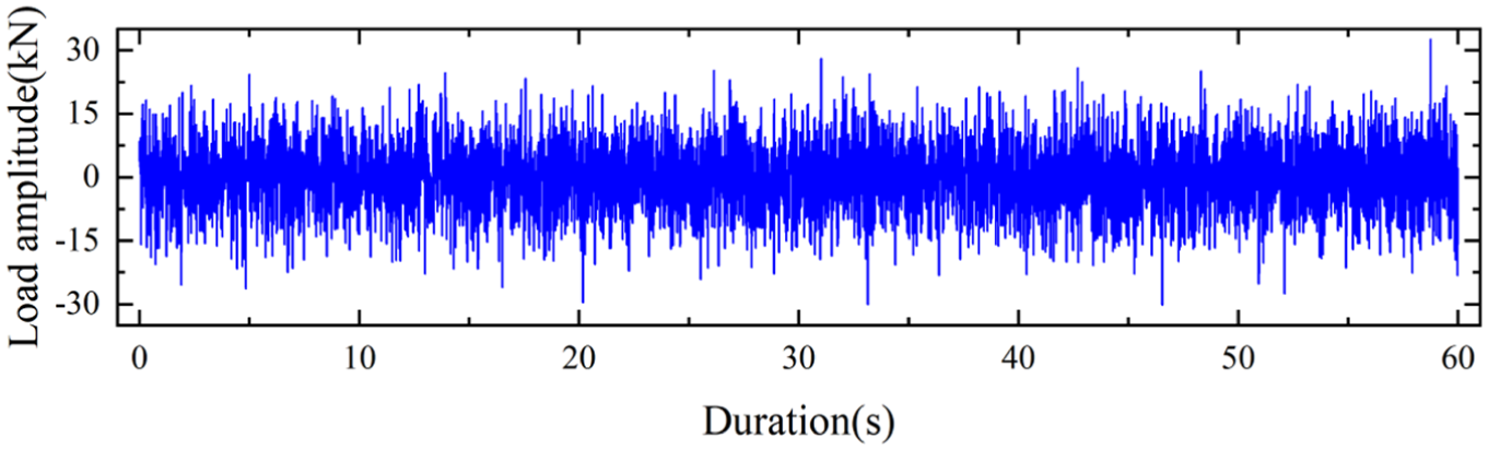
Gaussian white noise loading.
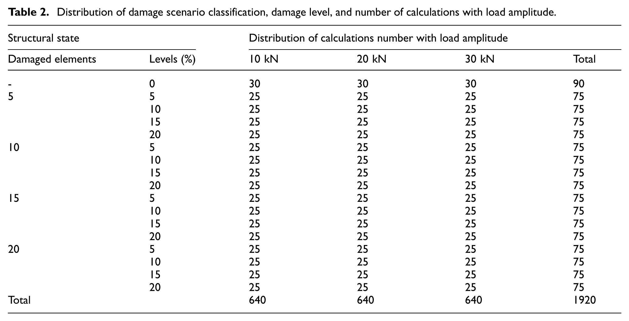
The distribution of damage location, damage levels, and the number of calculations corresponding to different load magnitudes are presented in Table 2. In this study, a total of R = 1290 finite-element calculations were performed. For each condition, the beam structure corresponds to an N-dimensional time-series dataset, where N (N = 7) refers to the number of measurement points. The acceleration sampling frequency was configured at 300 Hz, balancing computational accuracy with reduced data volume through optimized sampling rate selection. Resulting in each acceleration dataset containing L = 60 × 300 = 18,000 values. However, in the Transformer model, the complexity of computations is proportional to the square of the sequence length being processed. 30 Therefore, to reduce the computational complexity and avoid significantly increasing computational cost, it is necessary to preprocess the original acceleration sequences.
Distribution of damage scenario classification, damage level, and number of calculations with load amplitude.
Data preprocessing
Data preprocessing utilizes a variety of data analysis techniques to process raw data, transforming it into a more suitable form for subsequent processing, improving the quality and usability of the data, as well as facilitating model training and improving model performance. 50
Normalization of data
Feature scaling of data while training neural networks is a very critical step. Especially in the case of multifeature data, where each feature has a different range, this results in higher computational costs and reduced model performance.51,52 This study employs Z-score standardization to process the data, ensuring that the standardized data have a mean of 0 and a standard deviation of 1. This removes the dimensional differences between features and ensures equal weight across them. Z-score standardization is calculated using the following formula:
where X refers to the raw data, μ is the mean value, σ represents the standard deviation, and X′ denotes the data after standardization.
Data augmentation and dataset partitioning
The sample distribution for this study is detailed in “Numerical simulation” section. In task 1 of the MTT-based model, the distribution of training data is imbalanced across different classes. The number of samples representing the healthy condition is significantly lower than that for other damaging conditions. This imbalance consequently leads the model to prioritize the class with a larger sample size during training, resulting in degradation of model performance. To address this issue, data augmentation techniques53,54 are used to process response data of healthy structures to increase the sample size for healthy conditions. Data augmentation improves sample balance and reduces the risk of overfitting. It also decreases reliance on original data and enhances training efficiency.
Random slicing is applied to the collected acceleration data, where segments are randomly selected from the original sequence to generate new response data. Sample partitioning is then performed to increase the number of samples representing healthy conditions and mitigate data imbalance. Specifically, two different continuous slices of length 16,000 are randomly selected from each standardized healthy sample to alleviate the issue of excessive sample distribution bias. Subsequently, to prevent data leakage caused by overlap and strong correlations among segments originating from the same run, the dataset is first partitioned at the level of simulation ID/test run (i.e., damage case): entire runs are assigned to the training, validation, and test sets before any slicing is performed. After this run-level split, random slicing is conducted only within each subset to generate segments, ensuring that no segments from the same original acceleration sequence appear across different subsets. Accordingly, 80% of the runs are used for training, while 10% are allocated for validation and 10% for testing.
This strategy enhances the model’s generalization by improving adaptability to unseen scenarios. Random slicing mimics the stochastic nature of sensor measurements in practical engineering, such as vibration signals across different time periods, thus ensuring high test accuracy. It also strengthens robustness to noise, as data augmentation drives the model to capture local signal variations, for example, differences induced by slicing positions, thereby increasing noise tolerance. Furthermore, the method extends applicability across diverse structures and excitations, demonstrating stable performance under conditions such as Gaussian white noise and hammer impacts.
Division of data
The long sequence data are divided into short sequence data samples of a window size using the OPE technique described in “OPE technique” section. The length of the original data is L, the size of the used window is window-size, and the sliding distance is step-size. Then, the number of samples that can be obtained from each analysis of the N-dimensional sequence data is q = [(L − window-size)/step-size] + 1. The total number of samples can be expressed as Q = q × R, where R refers to the number of original data pieces. The overlap rate of the sliding window is ρ = (window-size − step-size)/window-size, which splits the raw data into overlapping segments for the purpose of reducing information loss and capturing the information in the signal comprehensively.
In the numerical simulations, a window size of 900 samples is adopted according to the sampling frequency of 300 Hz, corresponding to a time duration of 3 s. This window length fully encompasses multiple vibration cycles associated with the first two natural frequencies of the simply supported beam (2.097 and 8.398 Hz), covering approximately 3–25 vibration periods. As a result, the selected window is sufficient to capture damage-induced variations in the dynamic response while avoiding the loss of critical modal information that may arise from excessively short time windows.
Training of the model
The configuration of various parameters during the model training process is presented in Table 3. The model was trained for 200 epochs, and the early stopping technique was employed to prevent overfitting. This technique controls the training process by monitoring changes in the evaluation metrics on the validation set. When the evaluation metric does not improve for a specified number of epochs beyond a predefined threshold, the model’s parameters are saved at that point, and training is terminated. This study used accuracy, precision, and recall as metrics for assessment. Combining these metrics allows for a comprehensive assessment of the model’s performance. The Adam optimizer was utilized for gradient updates during training, which allows for rapid exploration of the parameter space with a larger learning rate in the early stages, enabling the model to quickly move toward the optimal solution and thereby accelerating convergence. Additionally, the learning rate decay curve is illustrated in Figure 6. The piecewise decay adjustment method is employed, the learning rate is adjusted to 90% of its original value every 50 epochs, with an initial learning rate of lr0 = 0.00005.
Configurations of the MFMTT model in training.
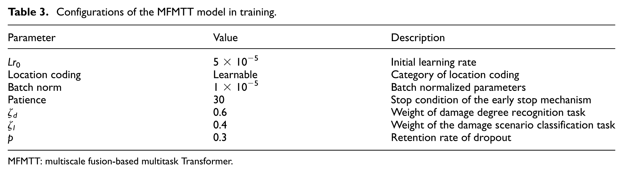
MFMTT: multiscale fusion-based multitask Transformer.
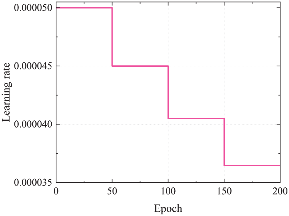
Learning rate decay curve.
The model’s hyperparameters were optimized through random search, which explores parameter combinations by sampling from predefined distributions. The final optimal hyperparameter configuration is presented in Table 4.
Hyperparameters of MFMTT model.
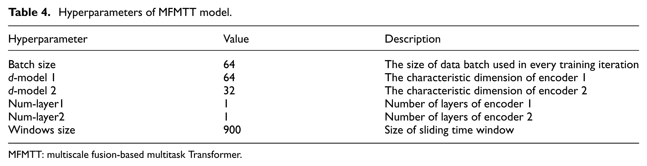
MFMTT: multiscale fusion-based multitask Transformer.
Single damage detection
In this section, the MFMTT is utilized for detecting and localizing different levels of structural damage in beams, and the results are compared with the results of a Transformer-based single-task model for this SDD task. A workstation with a Windows 10 operating system equipped with an NVIDIA RTX A5000 GPU was used to train the model.
Damage detection model of different feature extractors
To validate the effectiveness of the proposed MFMTT, a comparative analysis was conducted with four damage detection models that incorporated distinct feature extractors while maintaining identical classifier architectures. The models are as follows: (1) Simple CNN (SCNN): A baseline model employing standard convolution layers for local feature extraction. (2) One-dimensional CNN (1DCNN): Utilizes one-dimensional convolutional operations to process temporal sequence data from structural response signals. (3) MTT: A Transformer architecture incorporating parallel task-specific decoders for simultaneous damage scenario classification and severity assessment, which lacks the multiscale feature fusion module compared to the MFMTT. (4) Multiscale Single-task Transformer (MST) Model: It extracts hierarchical features through dilated convolutions with varying dilation rates, but focuses exclusively on damage classification rather than MTL. The hyperparameter configuration of all models in the training process is the same as shown in Table 3.
The damage detection results of different models
The loss curve during model training is shown in Figure 7. The loss curve converges to a stable plateau before training termination, indicating that the model reaches convergence without observable overfitting. Therefore, the hyperparameter settings at this point are appropriate.
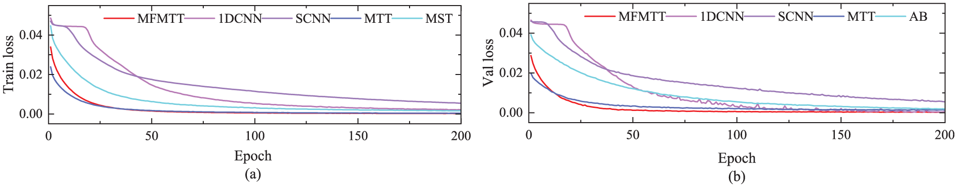
Loss curves: (a) training set and (b) validation set.
After training completion, the accuracy curves of the MFMTT, MTT, MST, 1DCNN, and SCNN models on both training and validation sets are illustrated in Figure 8. As shown in the figure, among the five models, the MFMTT model achieves the optimal state most rapidly, converging after 50 epochs and exhibiting stable performance with negligible variation after 75 epochs. The multitask model MTT converges at the second-fastest rate. Although its precision is higher than that of the MFMTT during the first 25 epochs, its improvement is slower than the MFMTT’s. It is not until after 100 training epochs that its performance becomes comparable to the MFMTT, while still being noticeably better than the other three models (MST, 1DCNN, SCNN). This demonstrates that MTL enhances the model’s capability to accurately identify structural damage. Furthermore, the Transformer-based MST model also surpasses SCNN and 1DCNN, indicating that integrating multiscale feature fusion with the Transformer architecture improves SDD compared to traditional CNNs. The confusion matrices of the MFMTT and MTT on the testing set are presented in Figures 9 and 10 respectively. The diagonal elements quantitatively represent the true positive cases, where predicted labels match the ground-truth annotations, while off-diagonal entries indicate misclassified samples with label discrepancies. As demonstrated in the figure, both models achieved robust classification performance with minimal prediction errors, thereby validating the reliability of their damage identification capabilities.
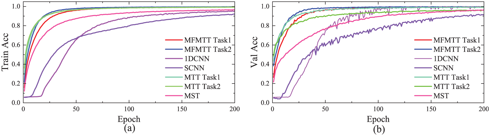
(a) Accuracy curves on training set and (b) accuracy curves on validation set.
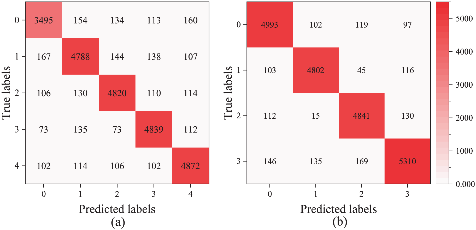
Confusion matrix of MFMTT on test set: (a) task 1 and (b) task 2. MFMTT: multiscale fusion-based multitask Transformer.
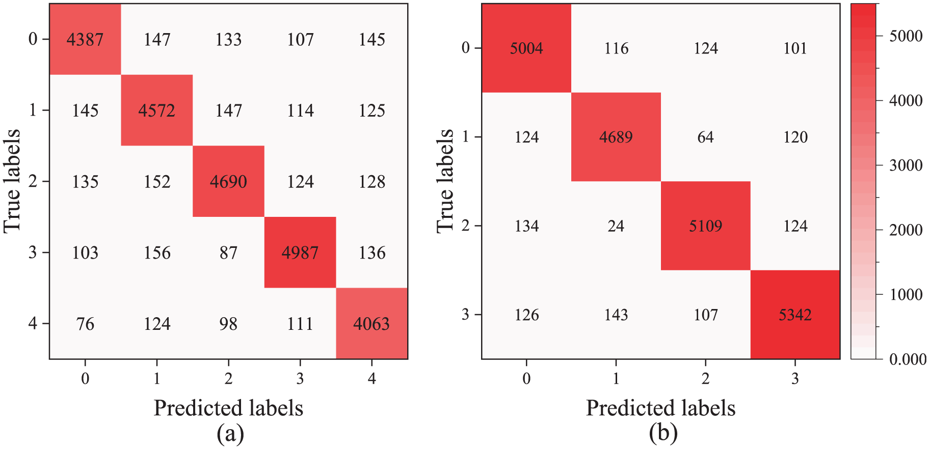
Confusion matrix of MTT on test set: (a) task 1 and (b) task 2. MTT: multitask Transformer.
Table 5 presents the accuracy of the above five models on the test set. The MFMTT model achieved the highest accuracy rates of 97.74% for damage severity identification and 96.74% for damage scenario classification, demonstrating superior performance in both classification and spatial recognition tasks.
Accuracy of different models’ structural damage identification results on the test set.
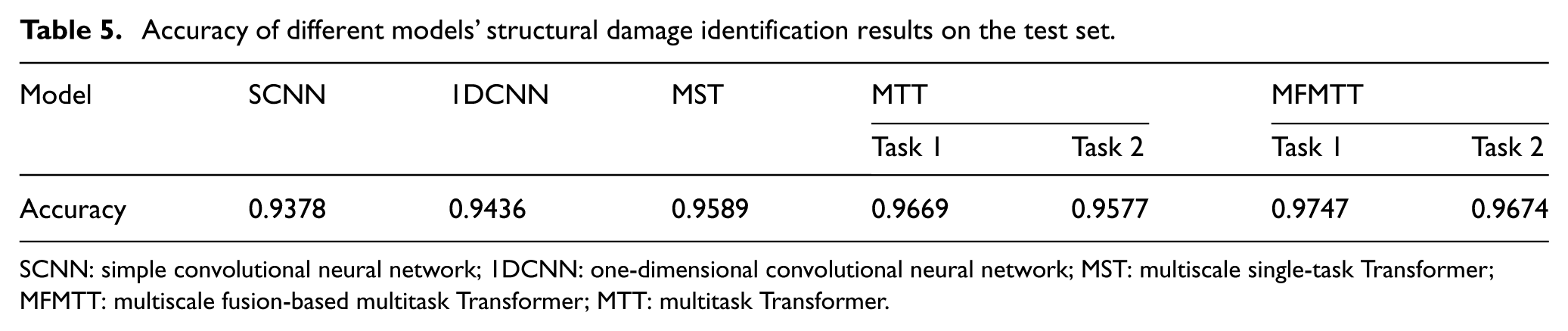
SCNN: simple convolutional neural network; 1DCNN: one-dimensional convolutional neural network; MST: multiscale single-task Transformer; MFMTT: multiscale fusion-based multitask Transformer; MTT: multitask Transformer.
To ensure the fairness of comparison, Table 6 summarizes the number of parameters and the samples computed per second after training for all models. Although the MFMTT has a longer training time due to overlapping-patch embedding and multiscale fusion, its parameter count (1.04 M) remains moderate and is significantly smaller than the MMT (3.82 M) baseline. This indicates that the superiority of the MFMTT does not arise from a larger model capacity. Instead, the performance gains stem from the architectural improvements, including multiscale feature integration and the task-filtered multitask formulation.
Comparison of model size and training cost across baseline models and the proposed MFMTT.
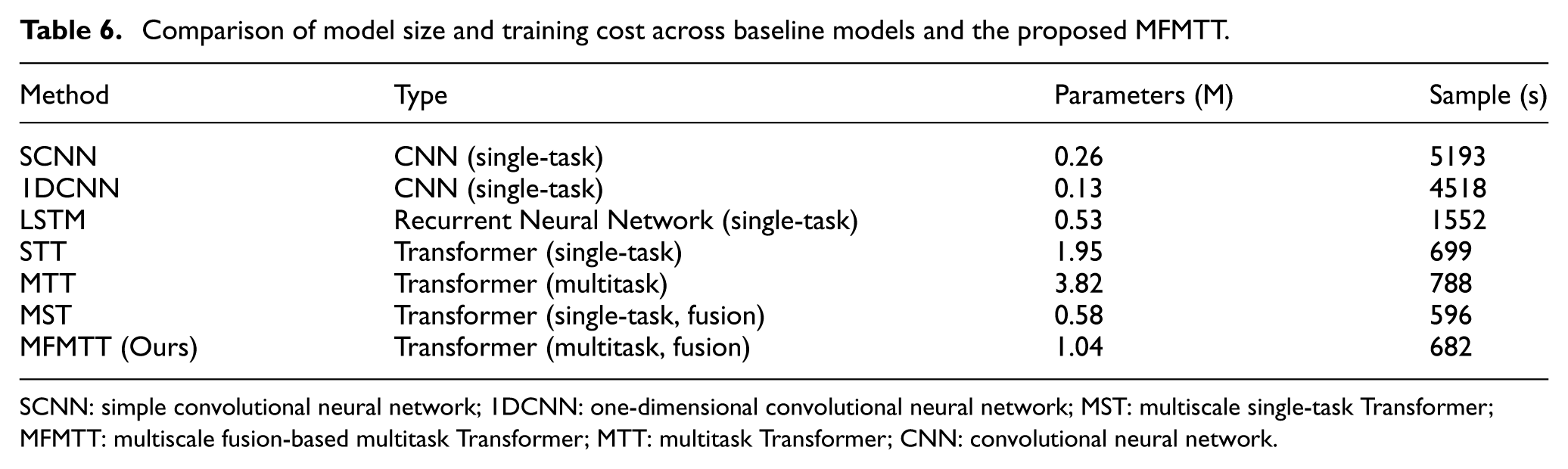
SCNN: simple convolutional neural network; 1DCNN: one-dimensional convolutional neural network; MST: multiscale single-task Transformer; MFMTT: multiscale fusion-based multitask Transformer; MTT: multitask Transformer; CNN: convolutional neural network.
Multiple damage detection
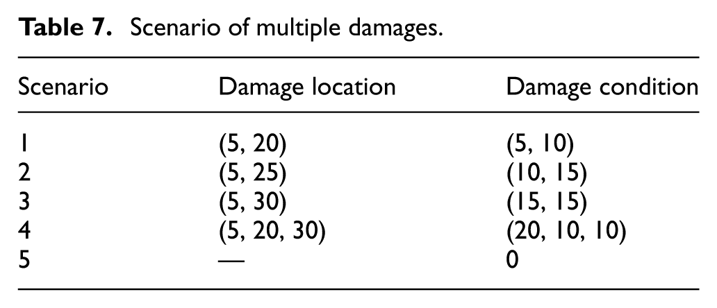
This section discusses the performance of the MFMTT model in detecting damage when multiple damages occur. Specifically, scenarios involving up to three simultaneous damages are considered, with the damage levels set to the five described in “Numerical simulation” section. All damage scenarios are presented in Table 7.
Scenario of multiple damages.
In order to obtain sufficient damage data, multiple calculations were performed on the simply supported beam mentioned in “Numerical simulation” section. As a result, similar to the single damage scenario, 75 calculations were conducted for each situation. Subsequently, the data obtained were divided into three datasets according to the method described in Section 3.2: 80% for training, 10% for validation, and 10% for testing.
The training curve for the MFMTT model used for multidamage identification is shown in Figure 11. This curve demonstrates a gradual convergence without signs of overfitting, which indicates that the MFMTT model is effective in recognizing multiple damage scenarios. Figure 12 presents the accuracy curves of the model across both training and validation sets. After 100 training epochs, the accuracies for task 1 and task 2 are 98.65 and 98.76%, respectively. Furthermore, Figure 13 presents the confusion matrix for the multidamage identification task on the test set. As illustrated, the majority of the elements lie along the diagonal, which signifies that the MFMTT model can accurately assess multidamage situations. Consequently, the MFMTT accurately identifies both the location and severity of structural damage.
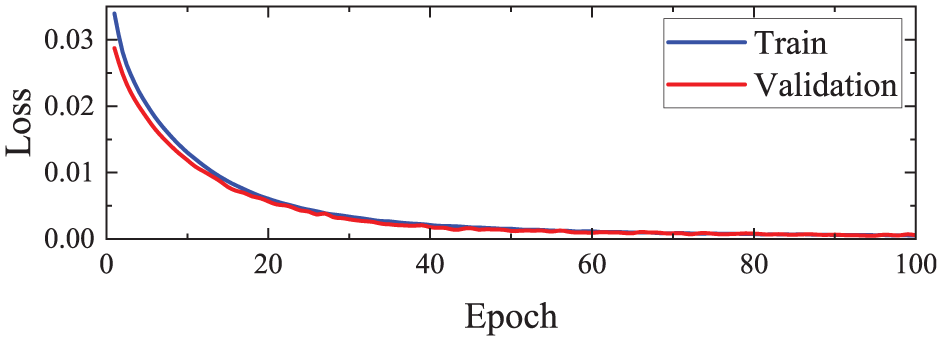
Loss curves for training and validation sets.
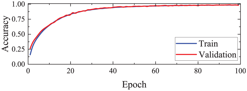
Accuracy curves on the training and validation sets.
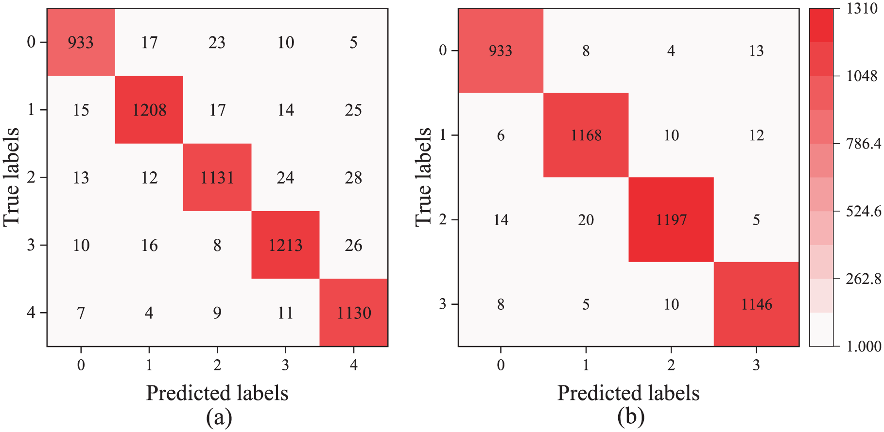
Confusion matrix on the test set: (a) task 1 and (b) task 2.
Noise effect on damage detection
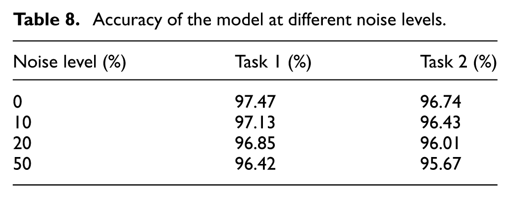
Noise, as a common input interference, may significantly affect the prediction accuracy and generalization ability of the model. This section aims to explore the impact of different noise levels on the performance of DL models to assess the robustness of the model in uncertain environments. Gaussian white noise was selected as the input interference in the experiments, and Gaussian white noise was achieved by adding randomly generated Gaussian-distributed noise to the raw input data. Gaussian white noise can be expressed by the formula: Xnoisy = Xclean + σ·N(0, 1). Xclean represents the original noise-free data. σ is the noise amplitude coefficient, which is used to control the noise level. In this paper, the noise intensity is described by noise level percentage, which is based on the ratio of the noise standard deviation σnoise to the standard deviation of the original data σclean. Three noise levels were considered: σnoise/σclean = 10%, 20%, 50%, corresponding to different standard deviations (σ = 0.1, 0.2, 0.5), to assess their impact on model performance.
Table 8 shows the accuracy of the MFMTT model on the training set at different noise levels. The corresponding bar chart is shown in Figure 14. It should be emphasized that the noise robustness assessment conducted in this study is restricted to additive Gaussian white noise with prescribed intensity levels. Within this controlled disturbance setting, the proposed MFMTT maintains stable classification performance even under relatively high noise ratios. Nevertheless, these observations should not be interpreted as evidence that noise effects are insignificant in practical SHM scenarios.
Accuracy of the model at different noise levels.
Accuracy of the MFMTT model under different noise levels. MFMTT: multiscale fusion-based multitask Transformer.
Experimental verification
Benchmark experiment
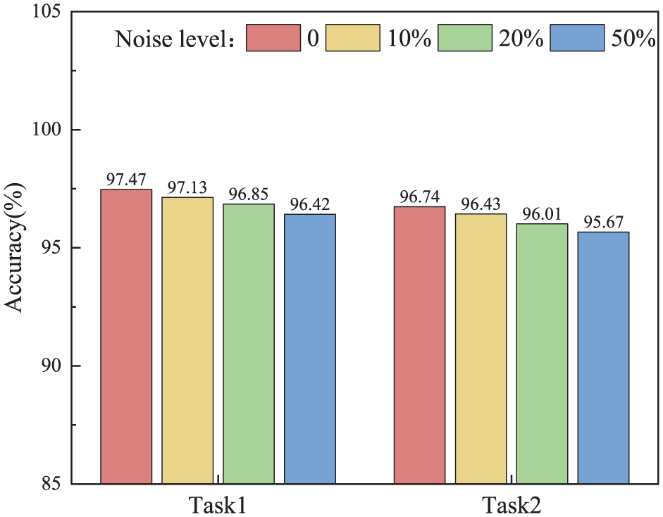
The second phase benchmark structure experiment of IASC-ASCE was conducted by the SHM Working Group based on the first-phase benchmark finite-element structure, 55 which took place at Columbia University in 2000. The framework structure of the experiment is shown in Figures 15 and 16.
IASC-ASCE two-stage structure. 55
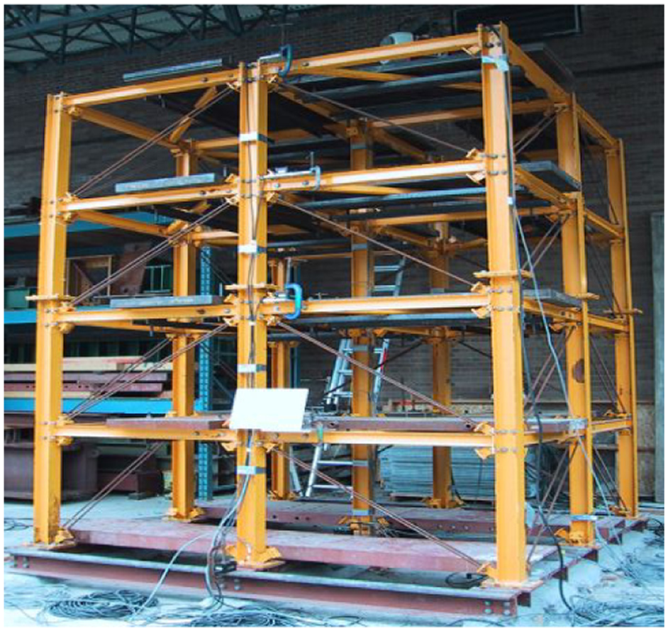
Exciter and acceleration sensor. 55
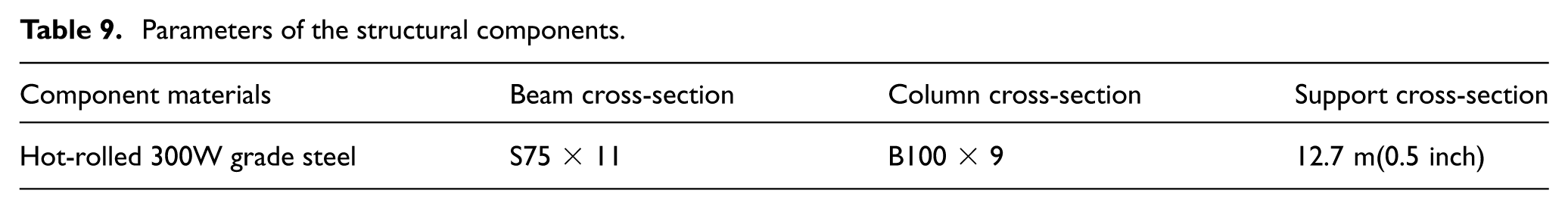
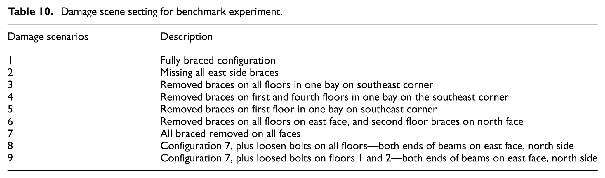
The structure stands 3.6 m high, with a planar dimension of 2.5 × 2.5 m, and consists of a two-span, four-story steel framework. Each level accommodates four identical steel plates, with the total mass of the steel plates on the first three levels being 4000 kg, and the total mass of the steel plates on the fourth level being 3000 kg. The diagonal supports utilize threaded rebar, and detailed parameters of the structure’s components are provided in Table 9. The damage scenarios in the experiment are set as shown in Table 10, and the damage was set up by removing the support and loosening the bolts. The data recorded during the testing of the University of British Columbia structure, a video of the experiment, and a complete description of the experimental setup are available on the ASCE SHM Task Group’s web page. 56
Parameters of the structural components.
Damage scene setting for benchmark experiment.
In this study, multilocation damage is addressed via a categorical labeling strategy rather than a multilabel formulation. For task 1, damage severity labels in finite-element simulation experiments are determined based on the stiffness reduction at the structure’s damaged nodes. Five damage levels are defined, corresponding to elastic modulus reductions of 0, 0.05, 0.1, 0.15, and 0.2, respectively. In the IASC-ASCE benchmark experiment, severity classes are delineated by the location and quantity of removed bracing members as well as the loosening degree of bolted connections; class 0 denotes a healthy condition, while all other classes correspond to distinct damage states. For task 2, each predefined multilocation damage configuration is treated as an independent class and assigned a unique categorical label. On this basis, multilocation damage scenarios in the IASC-ASCE benchmark, such as damage scenario 6, are encoded as individual damage configuration classes. This labeling strategy eliminates ambiguity in representing multilocation damage and aligns with the standard formulation of the IASC-ASCE benchmark, thereby ensuring clarity and reproducibility within the proposed multitask framework.
Acceleration sensors are installed on the east central column, west central column, and structural central column of each floor (including the foundation) of the structure. Therefore, the collected structural acceleration responses contain data from 15 channels. As shown in Figure 16, the exciter and the accelerometer were used. The data acquisition frequency was 200 Hz, and the white noise excitation lasted for 120 s. The acceleration excitation generated by the exciter is shown in Figure 17.
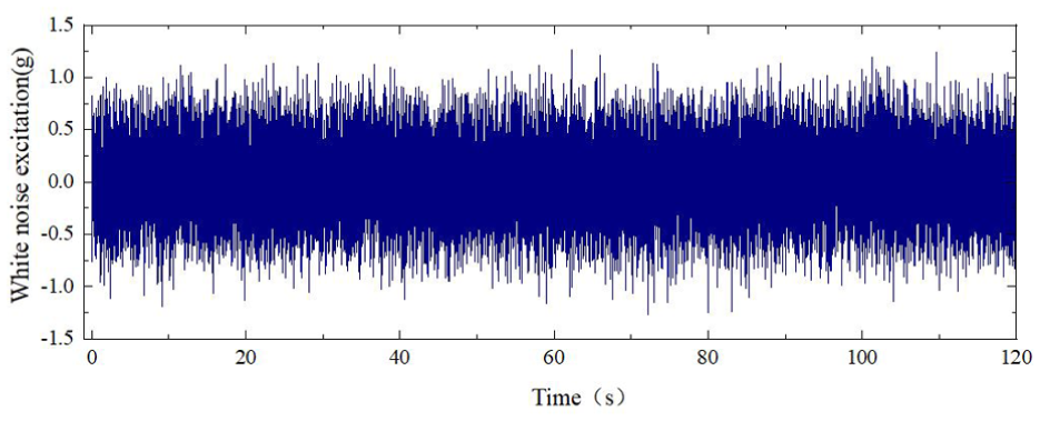
Baseline experiment with Gaussian white noise excitation.
Using data augmentation techniques, random slices of standardized data were generated to obtain more damage data. The data slices were configured with a length of two-thirds of the shortest sequence, where each segment contained 60,000 time steps to ensure uniform sampling intervals. These data were then divided into training, validation, and test sets in an 8:1:1 ratio, and the model’s performance was validated on these datasets.
Result of damage detection on the benchmark experiment
The loss curve of the MFMTT model training is shown in Figure 18. As can be seen from the figure, the value of the loss function of the model no longer decreases significantly after 30 training epochs. When approaching 60 epochs, the value of the loss function remains basically unchanged, and the curve is close to a horizontal line before the training stops. There is no overfitting on the validation set, indicating that the training result of the model is valid. The damage detection results are presented in Table 11. The accuracy of damage detection can reach approximately 98% on the training set, and the validation set can reach approximately 97%. The curves of accuracy, precision, recall, and F1-score for the two tasks on the training and validation sets are shown in Figures 19 and 20. All curves tend to level off eventually, and there is no overfitting on the training set. Figure 21 shows the confusion matrix of the MFMTT model on the test set, and the elements in the figure are mostly distributed on the diagonal, indicating that the model reliably identifies each classification.
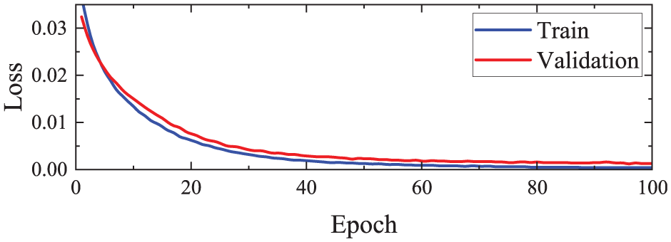
Loss curves on the training and validation sets.
Damage detection results of the baseline structure of the MFMTT model.
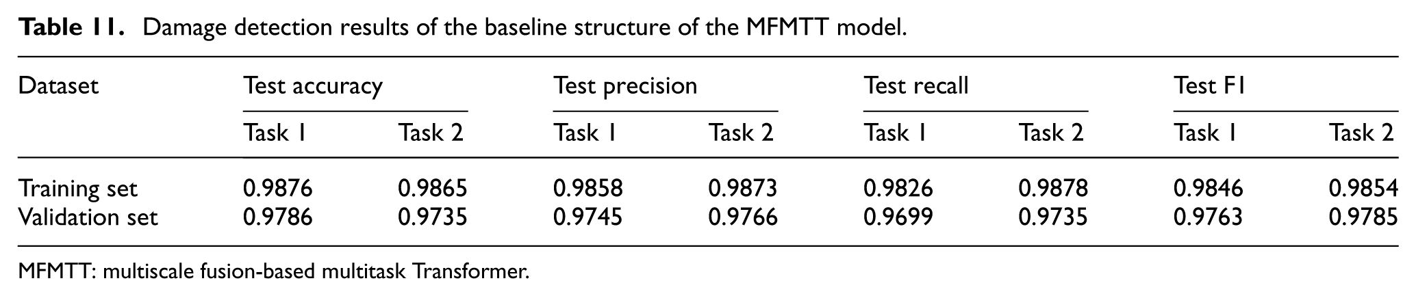
MFMTT: multiscale fusion-based multitask Transformer.
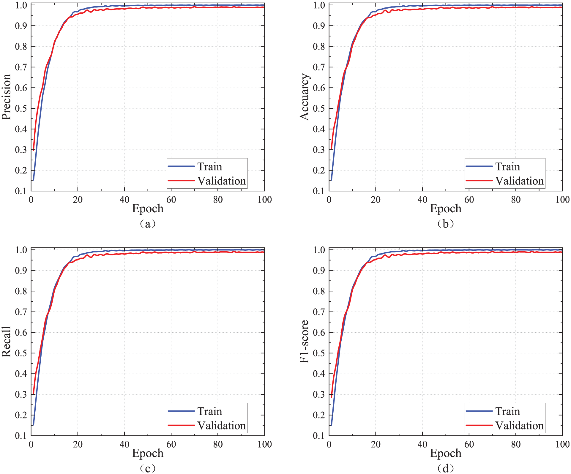
Damage severity recognition results: (a) precision, (b) accuracy, (c) recall, and (d) F1-score.
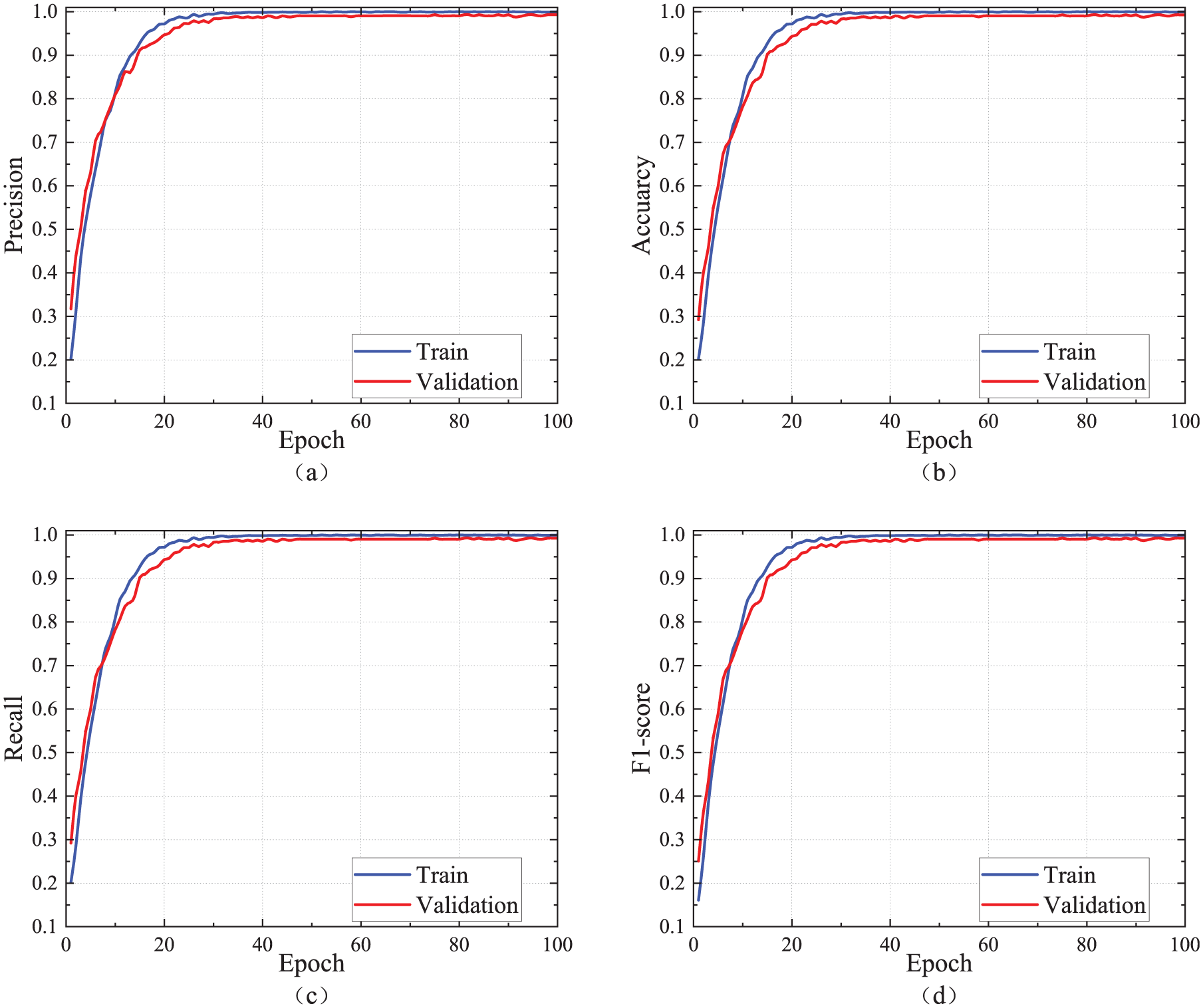
Damage scenario classification recognition results: (a) precision, (b) accuracy, (c) recall, and (d) F1-score.
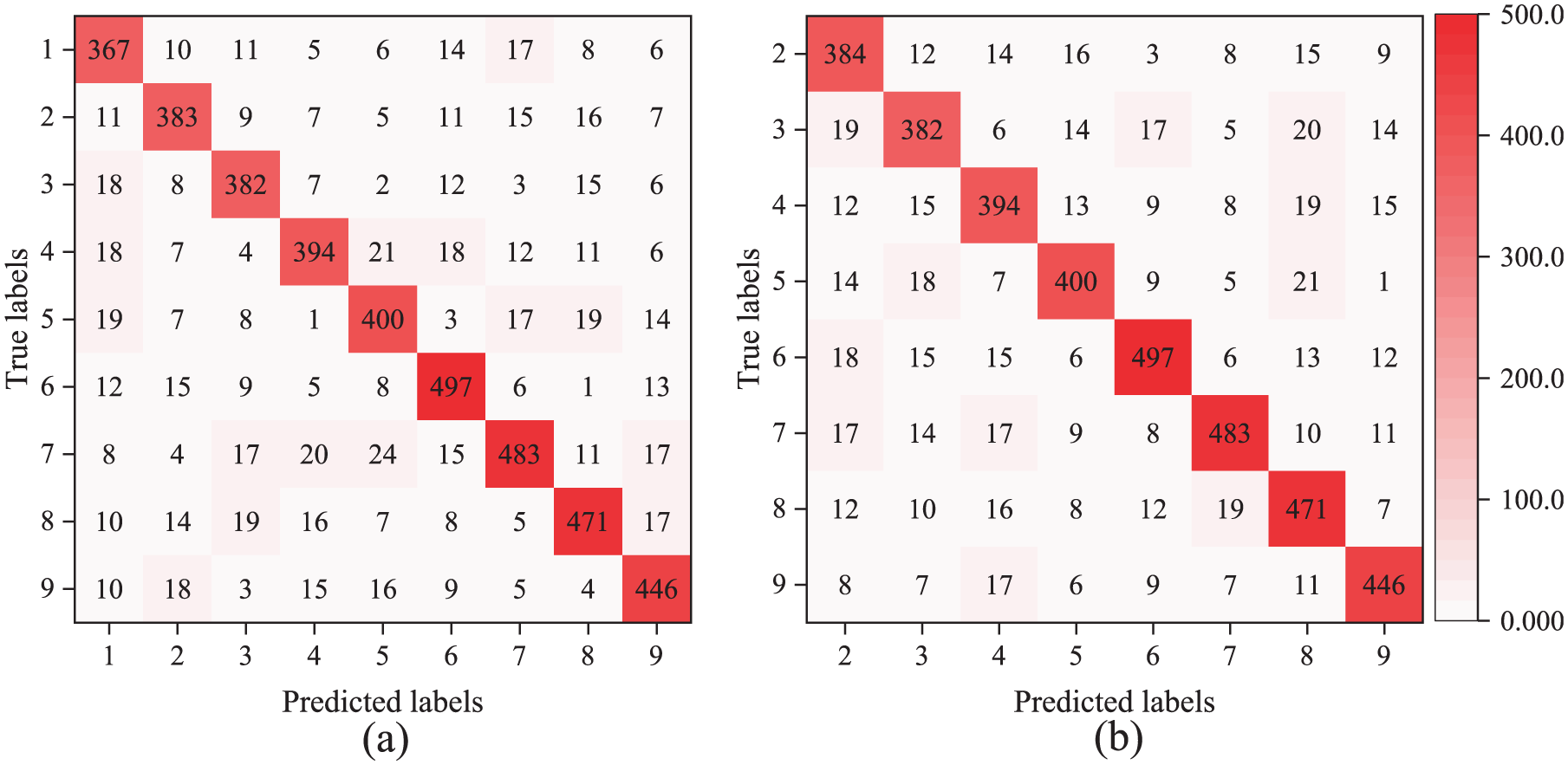
Confusion matrix on the test set: (a) task 1 and (b) task 2.
Conclusions
In this study, an MFMTT for SDD is proposed, which can obtain accurate structural damage predictions by utilizing acceleration response data at different scales of the structure. The MFMTT integrates a multivariate time-series Transformer network with multiscale dilated convolutions, combining global temporal dependencies and local multiresolution feature extraction. A dataset for model training is generated by conducting dynamic analyses on a finite-element model of a simply supported beam under various damage conditions. On this dataset, the proposed MFMTT demonstrated significantly superior performance, achieving a damage identification accuracy of 97.47% and a damage scenario classification accuracy of 96.74%. The superior performance of the MFMTT model over CNNs is clearly demonstrated by the experimental results. The performance of the MFMTT model in detecting damage under multiple damage scenarios was also examined. In these situations, the accuracy for identifying the severity of damage reached 98.65%, and the accuracy for the identification of the damage scenario classification was 98.76%. The noise robustness analysis presented in this work is confined to scenarios involving additive Gaussian white noise. In contrast, practical SHM systems are typically subject to a broader range of complex and nonstationary disturbances, including temperature fluctuations, wind loading, traffic-induced vibrations, sensor drift, and long-term environmental effects. As these sources of variability were not explicitly considered, the robustness of the proposed MFMTT under realistic operational conditions cannot be directly inferred from the current results.
In summary, this study highlights the potential of the proposed MFMTT model for SDD applications. The experimental investigations in this study are conducted under relatively idealized numerical and laboratory conditions. The numerical validation relies on a simply supported beam with a limited set of predefined damage scenarios and a single excitation type, while the benchmark experiments involve a restricted number of damage configurations under controlled testing environments. Consequently, variations in structural typologies, boundary conditions, stiffness distributions, and broader operational or environmental influences, including the effects of extreme events such as natural hazards, are not explicitly addressed. In addition, several practical challenges commonly encountered in real-world SHM applications remain beyond the scope of the present evaluation framework, including scalability to large-scale or geometrically irregular structures, the feasibility of real-time inference, robustness under complex and nonstationary environmental disturbances beyond synthetic Gaussian noise, as well as issues related to sensor malfunctions, missing data, and long-term environmental variability. While these limitations are acceptable for an initial methodological study aimed at assessing the feasibility and effectiveness of the proposed MFMTT framework, they suggest that caution is required when generalizing the present findings to operational structures. Future work will therefore focus on extending the proposed approach to more diverse structural systems and loading conditions, incorporating realistic environmental and operational variability, and systematically evaluating performance under incomplete or degraded sensing scenarios, to enhance both robustness and practical applicability.
Footnotes
Declaration of conflicting interests
The authors declared no potential conflicts of interest with respect to the research, authorship, and/or publication of this article.
Funding
The support from Basic and Applied Basic Research Foundation of Guangdong Province (Grant No. 2024B1515120032) and Guangzhou Science and Technology Program (Grant No. 2024D03J0021) is greatly appreciated.