A fault diagnosis method with continuous frequency-band indicator embedding and class-aware interpretable feature weighting

Abstract

Neural networks have been extensively applied in mechanical fault diagnosis due to their strong capabilities in feature extraction and classification. However, their limited interpretability and unknown credibility of decision hinder deployment in high-reliability scenarios. To address this issue, a frequency band multi-indicator feature embedding (FIE) method based on physical information embedding is proposed. A filter bank integrated into the convolutional layer is employed to simulate the spectrum, upon which multifrequency domain indicators are computed to extract multichannel physical features that vary continuously with frequency bands. A class-aware weight mask, enabling interclass distribution differentiation, is generated to assign distinct channel weights for different faults. This facilitates the extraction of key features for decision analysis and enables credibility evaluation based on a distance metric. Experimental results on multiple fault datasets demonstrate that the FIE module exhibits strong noise robustness and enhances diagnostic performance under variable-speed conditions. Furthermore, the class-aware mask supports reliable credibility assessment and feature interpretation, thereby supporting feature-level interpretation and decision credibility assessment while maintaining internal transparency.

Keywords

Fault diagnosis interpretability physical information frequency band feature indicators class-aware weight mask

Introduction

Mechanical fault diagnosis is essential for ensuring the safe operation of critical equipment and mitigating substantial economic losses. Traditional approaches are primarily grounded in model-driven or signal analysis theories, in which fault identification is achieved through physical simulation mechanisms or adaptive time–frequency analysis strategies.^1,2 Nevertheless, these methods are typically constrained by expert experience or prior model assumptions, and their generalization capability under complex and nonstationary conditions remains insufficient.

Deep learning models, due to their powerful data-driven capabilities and efficient convergence speed without requiring expert knowledge, have been widely applied in the field of fault diagnosis,^3,4 demonstrating superior performance. In recent years, diverse deep learning frameworks have been proposed to address cross-condition transfer, adaptive feature enhancement, and few-shot generalization. These approaches include unsupervised transfer methods based on dual pseudo-label selection, diagnostic models integrating multiscale convolution with attention mechanisms, and intelligent diagnostic strategies incorporating meta-transfer learning concepts.^5–7

However, mechanical components requiring fault diagnosis are often critical to system operation, imposing stringent reliability requirements on diagnostic methods.^8,9 Reliability in this context primarily involves model performance and interpretability. The data-driven diagnostic process typically comprises three stages: data acquisition, feature extraction, and fault classification,^10,11 where feature extraction plays a pivotal role in determining diagnostic performance.¹² Due to the intricate internal mappings and opaque data transformations within neural networks, these models are often perceived as “black boxes,” leading to challenges in trust and adoption for critical equipment maintenance tasks.¹³ Enhancing the interpretability of neural networks is therefore essential for gaining user confidence.

To enhance feature extraction, various network architectures incorporating convolutional structures^14,15 and attention mechanisms^16,17 have been proposed to process time-domain signals. Given the limited and disordered information in raw time-domain signals, preprocessing has been considered an effective strategy for feature enhancement. Features extracted by preprocessing modules often contain richer fault-related information, thereby improving the performance and efficiency of subsequent analytical models. Jiao et al.¹⁸ designed a branch-filtering-based pre-processing module to generate features for transformer-based analysis. Shang et al.¹⁹ proposed a wavelet-based denoising module to unify noise reduction and feature mining. Lu et al.²⁰ designs a wavelet packet energy encoder to embed energy information into the sample feature space. Li et al.²¹ employed a wavelet packet decomposition as a preanalysis module, with decomposition features fused with learned network features to enhance performance. Wang et al.²² combining spectral window masking and group convolution to produce features with directional fault characteristics. Liu et al.²³ introduced a signal-by-signal filtering module to adaptively extract fault-sensitive patterns from spectral data, significantly improving diagnostic accuracy. In the studies by He et al.,^24,25, convolutional kernels in the first layer were initialized with wavelet shapes and updated during training to extract rich time–frequency features. Lu et al.²⁶ designed a convolution-based module to generate analog envelope spectra, thereby improving model performance in domain adaptation scenarios.

Interpretability in deep learning has been pursued via two primary approaches: self-explanation and post hoc explanation. The former focuses on transparent model design and normative structure, while the latter interprets decision rationales after inference. Due to its nonintrusive nature, post hoc explanation initially gained popularity. Grezmak et al.²⁷ used layerwise relevance propagation to assess whether the model concentrated on distinct fault types. Chen and Lee¹³ applied local interpretable model-agnostic explanations to explain classification criteria. However, post hoc methods are limited to highlighting critical regions postprediction and cannot resolve the intrinsic opacity of neural mappings.

To achieve self-explanation, many efforts have focused on constructing inherently interpretable model structures and logically meaningful function mappings. Sanakkayala et al.²⁸ adopted SHapley additive explanations values to select decoupled neural basis functions as interpretable classifiers. Shen et al.²⁹ imposed constraints on feature map activation regions to ensure distinct group outputs. Nevertheless, excessive emphasis on structural transparency may hinder model adaptability under complex conditions. Consequently, embedding signal processing knowledge—offering explicit functional mappings—has attracted increasing attention. Ravanelli and Bengio³⁰ embedded sinc functions into convolutional kernels to extract spectral fault features. Zhu et al.³¹ incorporated wavelet kernels to preanalyze input signals. Li et al.³² reequationted wavelet packet decomposition as multilayer convolution to yield interpretable outputs. Feng et al.³³ used diverse wavelet kernel types and sizes to improve feature diversity. Emulating signal processing within neural architectures has also emerged as an effective self-explanatory strategy. Chen et al.³⁴ integrated real and imaginary components from signal analysis into network modules to generate comprehensive time–frequency representations. The aforementioned approaches construct modules with explicit signal processing semantics to impose structural physical constraints and extract physically meaningful feature representations. In fault diagnosis, these methods exhibit significant advantages in diagnostic performance and interpretability, and can be categorized under the broader field of physical information modeling. However, it’s important to note that they differ from the paradigm of physical information neural networks, which are equation-driven, aim to approximate physically consistent solutions in a continuous function space, and force network outputs to satisfy known physical laws.

In summary, the incorporation of signal processing knowledge into a feature processing module can enhance model performance and interpretability. However, such approaches typically rely on feature mining in the vibration time-domain signal, which is highly susceptible to domain shifts caused by varying environmental noise and operational conditions. These shifts often degrade diagnostic accuracy. In contrast, spectral representations offer more stable characteristics and richer features under such variations. Despite this, most existing studies focus only on spectral simulation. As a single-channel representation, the spectrum still requires further feature extraction to obtain fault features robust to changing conditions. Additionally, improvements in interpretability are mostly limited to self-explainability, which merely confirms that the model operates on certain physical or mathematical principles, without revealing the key features or criteria underlying classification decisions. Furthermore, current methods fail to address the critical issue of decision credibility in practical applications, as they cannot provide early warnings for potential misjudgments or assess the reliability of test results.

To address these limitations, an interpretable feature embedding method with explicit physical structure is proposed. Frequency-domain statistical indicators with clear signal processing semantics are embedded at the representation level. Discriminative features are learned within a physically interpretable space, where meaningful spectral trends and decision-relevant feature structures are preserved. The module conducts deep mining of multidimensional physical characteristics in the frequency domain, enhances robustness under varying noise and operational states, and ensures that extracted features possess clear physical meanings. Moreover, it provides key information influencing model decisions, offers interpretative insights into classification results, and enables assessment of model trustworthiness. The main contributions are summarized as follows:

A frequency band physic-indicator feature embedding (FIE) module with continuous physical information embedding is proposed. This module directly processes one-dimensional vibration signals and outputs multichannel physical features. It is plug-and-play and compatible with various convolutional networks.

The FIE module introduces regional traversal of multiple physical indicators on the frequency spectrum to extract frequency-dependent, multichannel embedding features. The computational mapping is constrained to retain physical significance. Experimental validation on multiple datasets confirms the stability and effectiveness of the features under changing environmental and operational conditions.

A class-aware weight masking mechanism is integrated into the FIE module, enabling the generation of distinct feature weight distributions for different fault types. This mechanism is embedded in the decision-making process, serving as a transparent basis for model classification and discrimination. It also supports reliability assessment through distance-based evaluations of the output.

The structure of this article is as follows: the second section introduces the theoretical foundation of the proposed method. The third section presents the model architecture and technical details. The fourth section demonstrates the advantages in performance and interpretability via benchmark evaluations. The fifth section concludes the study.

Preliminaries

FIR filter-based analog spectrum generation

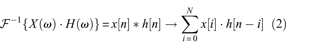
The finite impulse response (FIR) filter characterized by a FIR in the frequency domain. Bandpass filtering is performed by leveraging the property that the Fourier transform of a convolution equals the elementwise product of the individual Fourier transforms:

F {x (t) * h (t)} = F {x (t)} F {h (t)}

(1)

The operators F and F−1 denote the discrete-time Fourier transform (DTFT) and its inverse, respectively. H(ω) represents the frequency response of the filter, and X(ω) denotes the Fourier transform of the input sequence. Accordingly, the output of an Nth order FIR filter for an input x[n] is expressed as follows:

F^{- 1} {X (ω) \cdot H (ω)} = x [n] * h [n] \to \sum_{i = 0}^{N} x [i] \cdot h [n - i]

(2)

Here, ℎ[n] denotes the frequency-domain impulse response of the FIR filter, and * represents the one-dimensional convolution operator. The term ℎ[i] refers to the time-domain FIR filter coefficients. Given the centrosymmetric nature of the sinc function (sinc(x) = sin(x)/x) used in filtering. In the time domain, an Nth order FIR filter operation is equivalent to a Conv1D operation with a kernel size of N + 1 and the bias set to 0.

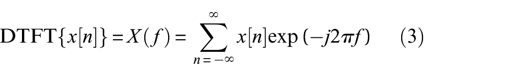
The DTFT is the most commonly employed spectral computation method. The DTFT of a discrete-time signal x[n] is denoted as X(f) and defined as follows:

DTFT {x [n]} = X (f) = \sum_{n = - \infty}^{\infty} x [n] \exp (- j 2 π f)

(3)

To integrate the spectral computation into neural network structures, the short-time Fourier transform (STFT), which performs window-based traversal, is adopted to approximate the DTFT. The discrete-time STFT is mathematically defined as follows:

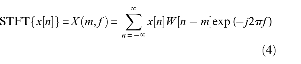
STFT {x [n]} = X (m, f) = \sum_{n = - \infty}^{\infty} x [n] W [n - m] \exp (- j 2 π f)

(4)

Here, x[n] represents the input sequence, X(m,f) denotes the STFT output, and W[n] is the window function.

Specifically, a Conv1D layer is constructed using a set of N-order FIR bandpass filters with adjacent center frequencies. Global maximum pooling (GMP) is then applied along the time axis to extract the dominant frequency component from each output channel, resulting in the analog spectrum. The implementation process is illustrated in Figure 1.

Figure 1.

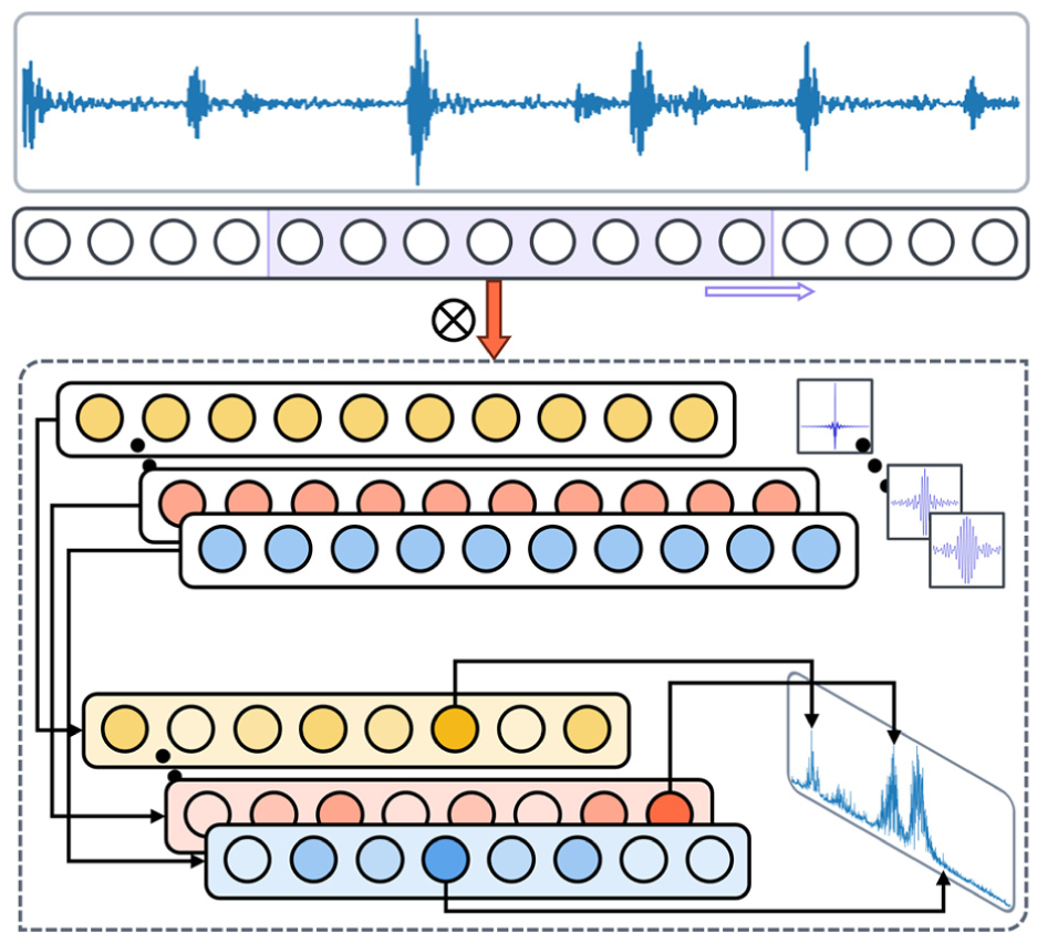
Acquisition of analog spectrum.

Triplet loss

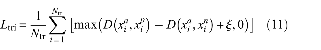
Triplet loss is a metric learning approach, designed to establish distinct feature boundaries by increasing intraclass compactness and interclass separability, thereby minimizing class overlap. Each triplet comprises an anchor sample $x_{i}^{a}$ , a positive sample $x_{j}^{p}$ , and a negative sample $x_{v}^{n}$ , where $x_{i}^{a}$ and $x_{j}^{p}$ belong to the same class, while $x_{v}^{n}$ belongs to a different class. Based on sample distances, triplets are categorized into easy, semihard, and hard types:

\begin{matrix} ‖ G (x_{i}^{a}), G (x_{j}^{p}) ‖ + ξ < ‖ G (x_{i}^{a}), G (x_{v}^{n}) ‖ \\ ‖ G (x_{i}^{a}), G (x_{j}^{p}) ‖ < ‖ G (x_{i}^{a}), G (x_{v}^{n}) ‖ + ξ \\ ‖ G (x_{i}^{a}), G (x_{v}^{n}) ‖ < ‖ G (x_{i}^{a}), G (x_{j}^{p}) ‖ \end{matrix}

(5)

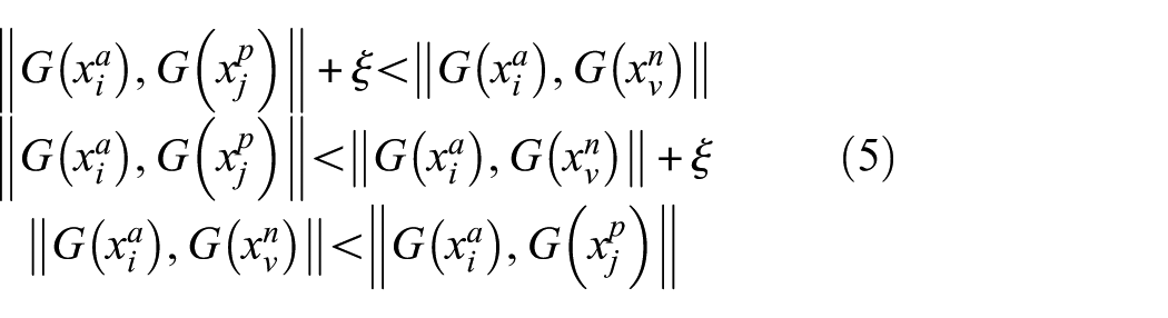
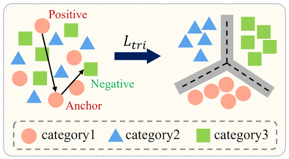
Here, ξ denotes a predefined margin, and G(⋅) represents the encoder for feature embedding. The objective of triplet loss is to ensure that the distance between $x_{i}^{a}$ and $x_{j}^{p}$ is smaller than that between $x_{i}^{a}$ and $x_{v}^{n}$ . Consequently, optimization primarily focuses on semihard and hard triplets. The principle of triplet loss is shown in Figure 2.

Figure 2.

Schematic diagram of triplet loss principle.

Proposed method

Spectrum information embedding method

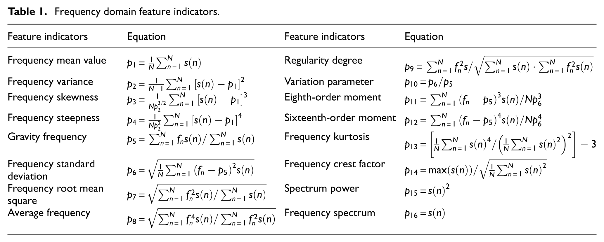
While the spectrum exhibits greater stability, information carried by single-dimensional features are limited. To enrich spectral information, two processing dimensions—channel expansion and regional frequency band—are considered. To ensure each expanded channel maintains a clear physical meaning, multiple frequency-domain indicator functions suitable for spectral analysis are selected (as listed in Table 1, where $s$ represents spectrum, $f$ represents frequency), enabling each output channel to represent a feature band associated with a specific indicator. To extract localized spectral features, a sliding window is applied to obtain spectrum segments that vary continuously across frequency bands. Each segment is processed using the selected frequency-domain indicator functions and reorganized by truncation order. Several frequency domain feature bands corresponding to each frequency domain indicator that change continuously with the frequency band can be obtained. These bands encode the spatial distribution of each indicator across corresponding spectral regions. The equation for generating overlapping frequency bands using the sliding window mechanism can be expressed as follows:

S_{k} = {X (s) | s \in [s_{k}, s_{k} + Δ s]}

(6)

where $s_{k} = s_{0} + k δ$ and $δ < Δ s$ . Since the step size $δ$ is less than the window width $Δ s$ , adjacent frequency bands share common spectral components. Therefore, the extracted feature values constitute a discrete continuous function with respect to the frequency indicator, where $p_{m} (\cdot)$ represents the mth frequency domain feature indicator:

I_{m} (k) = p_{m} (S_{k})

(7)

Table 1.

Frequency domain feature indicators.

Feature indicators	Equation	Feature indicators	Equation
Frequency mean value	$p_{1} = \frac{1}{N} \sum_{n = 1}^{N} s (n)$	Regularity degree	$p_{9} = \sum_{n = 1}^{N} f_{n}^{2} s / \sqrt{\sum_{n = 1}^{N} s (n) \cdot \sum_{n = 1}^{N} f_{n}^{2} s (n)}$
Frequency variance	$p_{2} = \frac{1}{N - 1} \sum_{n = 1}^{N} {[s (n) - p_{1}]}^{2}$	Variation parameter	$p_{10} = p_{6} / p_{5}$
Frequency skewness	$p_{3} = \frac{1}{{Np}_{2}^{3 / 2}} \sum_{n = 1}^{N} {[s (n) - p_{1}]}^{3}$	Eighth-order moment	$p_{11} = \sum_{n = 1}^{N} {(f_{n} - p_{5})}^{3} s (n) / {Np}_{6}^{3}$
Frequency steepness	$p_{4} = \frac{1}{{Np}_{2}^{2}} \sum_{n = 1}^{N} {[s (n) - p_{1}]}^{4}$	Sixteenth-order moment	$p_{12} = \sum_{n = 1}^{N} {(f_{n} - p_{5})}^{4} s (n) / {Np}_{6}^{4}$
Gravity frequency	$p_{5} = \sum_{n = 1}^{N} f_{n} s (n) / \sum_{n = 1}^{N} s (n)$	Frequency kurtosis	$p_{13} = [\frac{1}{N} \sum_{n = 1}^{N} s {(n)}^{4} / {(\frac{1}{N} \sum_{n = 1}^{N} s {(n)}^{2})}^{2}] - 3$
Frequency standard deviation	$p_{6} = \sqrt{\frac{1}{N} \sum_{n = 1}^{N} {(f_{n} - p_{5})}^{2} s (n)}$	Frequency crest factor	$p_{14} = \max (s (n)) / \sqrt{\frac{1}{N} \sum_{n = 1}^{N} s {(n)}^{2}}$
Frequency root mean square	$p_{7} = \sqrt{\sum_{n = 1}^{N} f_{n}^{2} s (n) / \sum_{n = 1}^{N} s (n)}$	Spectrum power	$p_{15} = s {(n)}^{2}$
Average frequency	$p_{8} = \sqrt{\sum_{n = 1}^{N} f_{n}^{4} s (n) / \sum_{n = 1}^{N} f_{n}^{2} s (n)}$	Frequency spectrum	$p_{16} = s (n)$

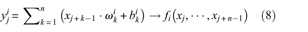
In the standard single-channel convolution layer, convolution is performed by elementwise multiplication between kernel parameters and the input, followed by accumulation. The operation of the ith kernel can be expressed as follows:

y_{j}^{i} = \sum_{k = 1}^{n} (x_{j + k - 1} \cdot ω_{k}^{i} + b_{k}^{i}) \to f_{i} (x_{j}, \dots, x_{j + n - 1})

(8)

As shown in Figure 3, the spectral embedding process is equivalent to convolving the spectrum with an indicator function serving as the kernel. This operation preserves the local continuity inherent to convolution, thereby ensuring smooth variation of embedded feature bands across frequency regions rather than forming independent and discontinuous descriptors. Consequently, each indicator channel encodes the local evolutionary trend of a specific statistical attribute along the spectral axis, thereby maintaining physical interpretability.

Figure 3.

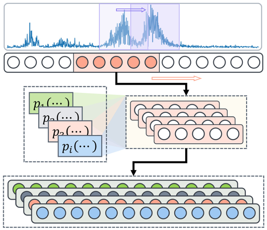
Calculation of indicator feature function based on spectrum.

From a signal processing perspective, this mechanism can be interpreted as a convolution between the spectrum and an indicator-based kernel that aggregates distributional information over adjacent frequency intervals. The overlapping window design imposes a local continuity constraint, whereby isolated spectral fluctuations are transformed into a progressively varying indicator trajectory.

Class-aware weight mask

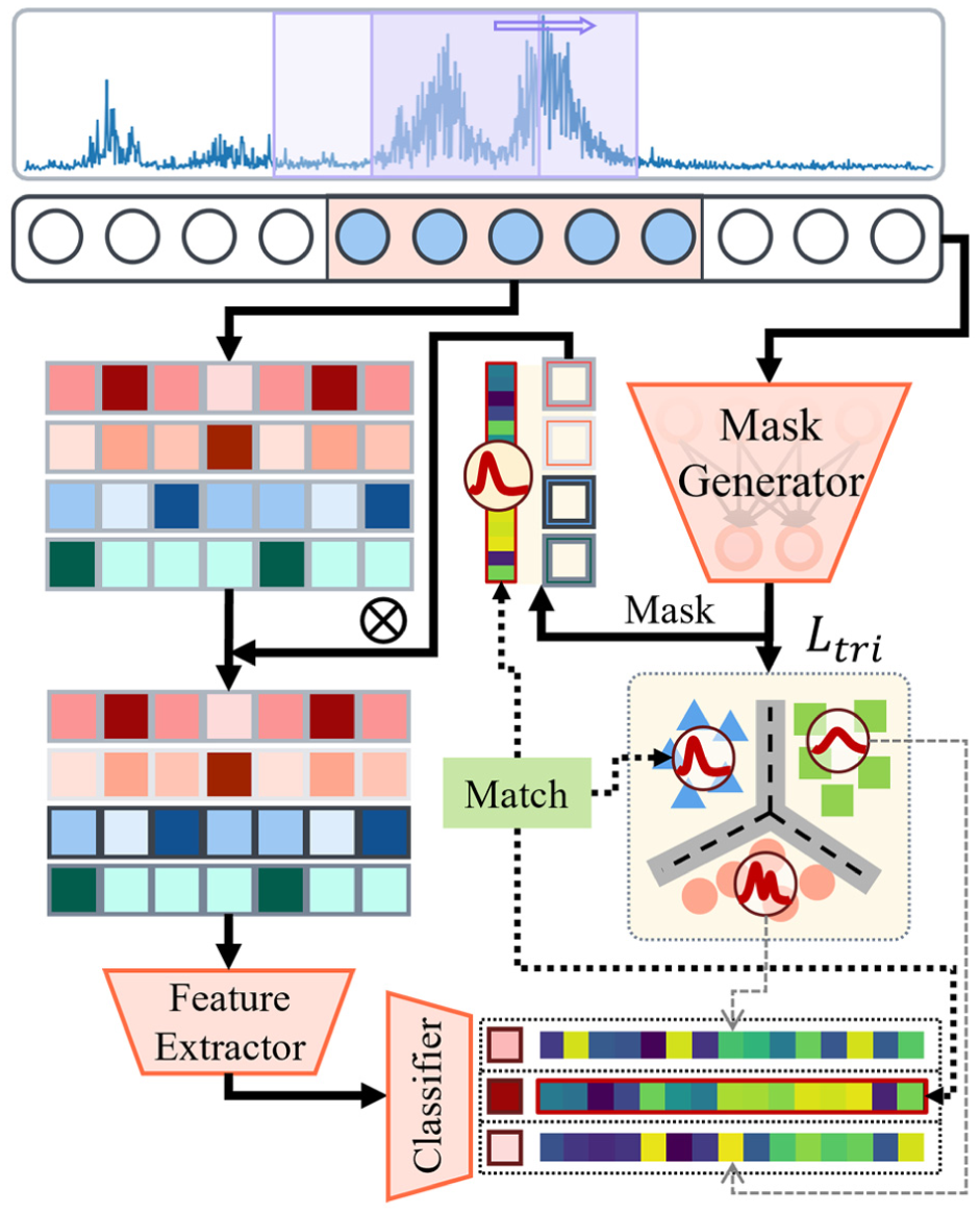
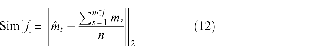
After extracting multiple spectrum feature bands representing each characteristic indicator, a class-aware weight mask is introduced to weight each channel. As illustrated in Figure 4, to facilitate network-wide interpretability, the generated weight mask is applied to each channel, followed by the computation of triplet loss. This process adjusts weight distributions by bringing those of the same class closer while increasing the separation between different types, ensuring distinct mask distributions for different health states. The Euclidean distance is utilized to measure distances between the two embedded sets:

D_{ij} = ‖ x_{i} - y_{j} ‖_{2} = \sqrt{\sum_{k = 1}^{d} {(x_{ik} - y_{jk})}^{2}}

(9)

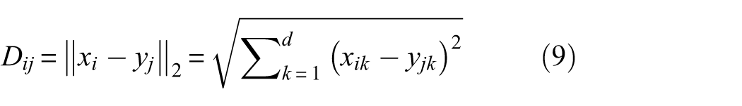
Where $x_{i}$ is the ith vector in the first set, and $y_{j}$ is the jth vector in the second set. Let $X \in R^{m \times d}$ represent the entire embedding set, which contains m d-dimensional vectors. The Euclidean distance calculation of its internal features can be simplified using matrix operations as follows:

D = \sqrt{X^{2} + X^{2} - 2 ({XX}^{T})}

(10)

Among them, $X^{2} \in R^{m \times 1}$ , $X^{2} \in R^{1 \times m}$ , and ${XX}^{T} \in R^{m \times m}$ . Therefore, let $N_{tr}$ represent the number of training set samples. The objective function of triple loss is defined as follows:

L_{tri} = \frac{1}{N_{tr}} \sum_{i = 1}^{N_{tr}} [\max (D (x_{i}^{a}, x_{i}^{p}) - D (x_{i}^{a}, x_{i}^{n}) + ξ, 0)]

(11)

Figure 4.

Class-aware weight mask operation.

Triplet loss effectively enforces similar mask distributions for the same class while maximizing distribution differences across different classes. Its optimization occurs concurrently with overall model training, embedding the weight mask into the model analysis process. This integration allows the weight mask to be incorporated into the model decision process, becoming an extractable key feature related to the model’s judgment category. From another perspective, this mechanism is equivalent to assigning different attention weights across channels. In implementation, the weight masks of each channel are designed to compete with each other through 0–1 standardization, compelling the model to select a limited number of feature channels as primary analysis targets for each health state. This strategy effectively aids subsequent analysis models in identifying key fault characteristics and further enhances the effectiveness of the output features generated by the prefeature analysis module.

Decision reliability judgment mechanism based on class-aware weight mask

Class-aware masks trained via triplet loss are characterized by intraclass consistency and interclass separability. Based on these masks and corresponding distance metrics, a decision reliability assessment method is proposed. In postanalysis, the Euclidean distances between the weighted mask ${\hat{m}}_{t}$ of a test signal and the center distributions of class masks are computed using Equation (12), where the jth element denotes the distance between the test sample and the center of the jth class mask. Moreover, a confidence threshold for Sim[j] is introduced to provide warnings of potential misjudgments under domain shift conditions.

Sim [j] = ‖ {\hat{m}}_{t} - \frac{\sum_{s = 1}^{n \in j} m_{s}}{n} ‖_{2}

(12)

The mask vector is defined as follows: $z = μ_{k} + ε, ε ~ N (0, Σ)$ , where $μ_{k}$ represents the center of the kth class and Σ denotes the noise covariance. Determination of the confidence threshold requires consideration of distribution shifts induced by domain drift. The threshold should not be strictly confined to the original distribution boundary, which would result in excessive rejection of samples with slight shifts. Conversely, an overly large threshold would weaken the misjudgment warning capability. Therefore, a trade-off between boundary expansion and preservation of class separability should be maintained. For categories with compact intraclass distributions, structural aggregation remains stable, and the threshold should not extend far beyond the source-domain boundary in order to preserve clear discrimination regions. For categories with loose intraclass distributions, aggregation is inherently weak in the source domain; excessive relaxation of the threshold would aggravate category overlap. Thus, even for loosely distributed categories, the threshold should primarily reference the discrimination boundary of compact categories to ensure consistency and robustness of the overall decision criterion.

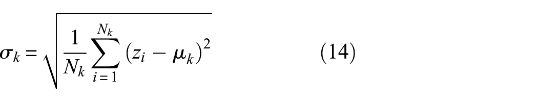
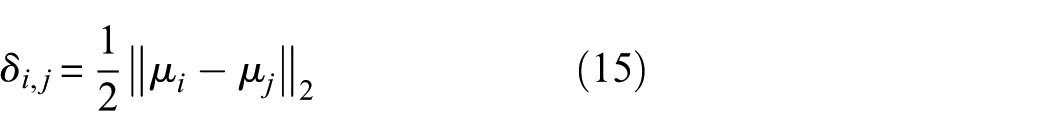
Based on the above considerations, we choose to use the “average midpoint” of the distance between the intraclass distribution sample boundary $r_{intra}$ and the interclass distribution $r_{inter}$ as the relevance threshold, according to Equation (13). This ensures a high acceptance rate for intraclass samples while minimizing the risk of confusion with the nearest heterogeneous class:

τ = \frac{r_{intra} + r_{inter}}{2} = \frac{1}{2} (\min_{k} \sqrt{d σ_{k}^{2}} + \sqrt{\min_{k} δ_{i, j}^{2} + \min_{k} d σ_{k}^{2}})

(13)

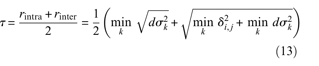
To ensure the applicability of the confidence threshold across different datasets, the training data are used to determine the Root Mean Square (RMS) noise $σ_{k}$ and the shortest half-distance $δ$ between different classes on the dataset using Equations (14) and (15), where $N_{k}$ is the number of training samples in the kth class.

σ_{k} = \sqrt{\frac{1}{N_{k}} \sum_{i = 1}^{N_{k}} {(z_{i} - μ_{k})}^{2}}

(14)

δ_{i, j} = \frac{1}{2} ‖ μ_{i} - μ_{j} ‖_{2}

(15)

The credible threshold serves two functions in misjudgment warning. (1) When the distance between the category mask of a signal and the center distribution of a specific class is significantly smaller than that of other classes and remains below the effective threshold, the selected indicator is considered highly consistent with the fault indicator of that class. The feature indicator selected by the mask explains the model decision and indicates high decision credibility for the sample. (2) When the distances between the signal mask and all class centers exceed the effective threshold, but the distance to the nearest class is smaller than that to other classes by at least one order of magnitude, the selected indicator remains more consistent with that class relative to others, and high decision credibility is retained. Through this indicator selection mechanism, features reflecting the network decision dependence are produced, and potential model misjudgments can be identified.

FIE module

The physical knowledge principles of the FIE module computation is illustrated in Figure 5. The overall process is summarized as follows:

An analog spectrum is generated by convolving the input time-domain signal with 600 filters of order 1000 and applied GMP to aggregate channelwise extrema, yielding an analog spectrum of length 600.

The normalized spectrum (range 0–1) is processed using the first 14 frequency-domain indicators listed in Table 1. A sliding window of size 15 is used for traversal, and the squared spectrum produces the 15th channel representing spectral energy.

A weight mask is generated by feeding the analog spectrum into a single-layer feedforward network (dropout rate = 0.5), producing weights for all 15 channels. Each channel is then standardized and weighted via broadcast multiplication. The triplet loss of the weight distribution is computed concurrently.

The 15 weighted channels are concatenated with the standardized spectrum to produce the final output features, which are forwarded to the diagnostic network. During training, the overall loss is composed of $L_{cls}$ and triplet loss $L_{tri}$ :

Loss = L_{cls} + μ L_{tri}

(16)

Figure 5.

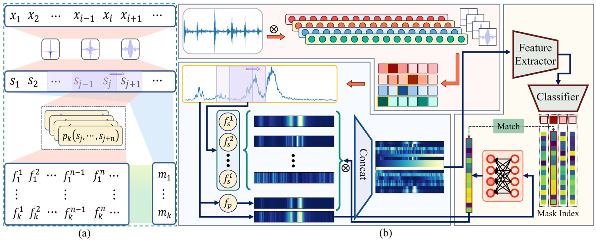
Overall calculation process of FIE method (left picture shows the physical knowledge principles of module). FIE: frequency band physic-indicator feature embedding.

Case study

In this section, four fault signal datasets are used to evaluate the proposed FIE under two scenarios, verifying its performance in fault diagnosis tasks. All data are segmented using a sliding window (window size = 2000, step size = 1000). The dataset test bench is shown in Figure 6, with details provided in Table 2.

Figure 6.

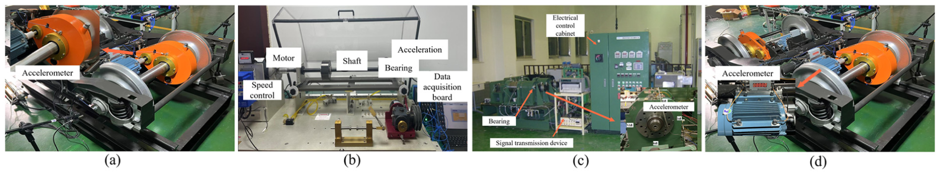
(a) RAOGB dataset test rig, (b) HUST dataset test rig, (c) BJTU dataset test rig, and (d) RAOMO dataset test rig.

Table 2.

Test dataset configuration.

Dataset	Classification	Fault type	Work scenario	Sample number
Dataset	Classification	Fault type	Work scenario	Train (per-class)	Test (per-class)
RAOGB	5 types	Normal, inner ring fault, outer ring fault, ball fault, cage fault	A: 20 Hz B: 40 Hz C: 60 Hz	50	100
HUST	4 types	Normal, inner ring fault, outer ring fault, ball fault	A: 20 Hz B: 40 Hz C: 60 Hz	50	100
BJTU	4 types	Normal, inner ring fault, outer ring fault, ball fault	A: 250 km/h B: 300 km/h C: 350 km/h	50	100
RAOMO	5 types	Normal, motor short circuit, broken rotor bars, bearing failure, bent rotor shaft	A: 20 Hz B: 40 Hz C: 60 Hz	50	100

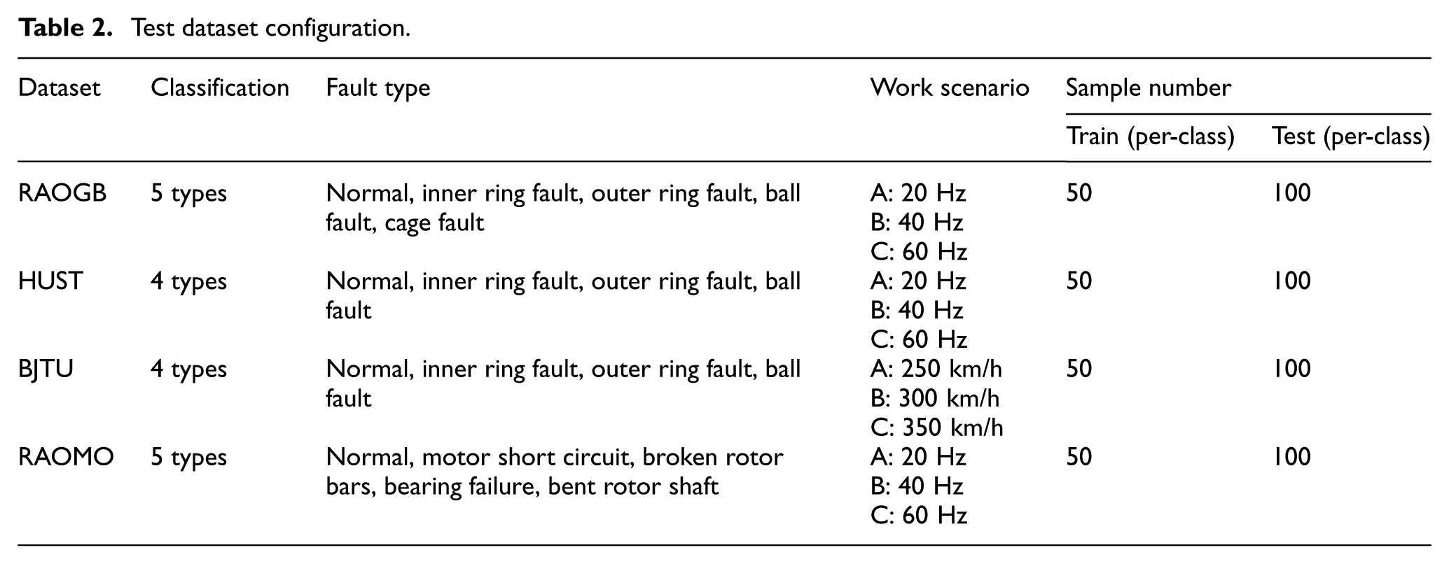
Noise scenario: Variations in environmental noise intensity affect signal distributions. Models trained on low-noise data often exhibit degraded or failed performance under high-noise conditions. To simulate this, training is conducted on 20 dB data, and testing is performed under increasing noise levels: 20/10, 20/2, 20/0, and 20/−2 dB. The SNR is defined in Equation (17). All samples are normalized using min-max normalization.

SNR = 10 \times \log_{10} (P_{s} / P_{n})

(17)

where $P_{s} = sum ({signal}^{2}) / len (signal)$ is the power of the input signal, and $P_{n}$ is the power of the noise to be added

Variable speed scenario: This test examines model performance under different rotational speeds after training at a single speed. As shown in Table 2, task A→B indicates training on data from scene A and testing on scene B. For comparison, results under no speed difference (A→A, B→B, C→C) are averaged as NV; results with small speed difference (A→B, B→A, C, C→B) are averaged as SV; and those with large speed difference (A→C, C→A) are averaged as LV. All samples are contaminated with 20 dB Gaussian noise and normalized using min-max normalization.

Each model is trained for 1000 iterations with an initial learning rate of 1e-3, decayed to 2e-4 using cosine annealing. The triplet loss weight factor μ follows exponential decay (initial value = 1, decay factor = 4). All experiments are implemented in Python 3.11 with PyTorch 2.3 and executed on an RTX 4060 GPU. Each test is repeated five times, and the average is reported. Accuracy measures the proportion of correctly predicted samples, while the F1-score represents the harmonic mean of precision and recall, defined as follows:

Accuracy = \frac{TP + TN}{TP + TN + FP + FN} \times 100 %

(18)

F 1 = \frac{2 \times TP}{2 \times TP + FP + FN}

(19)

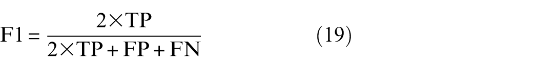
Among them, TP: predicted as positive and actually positive. TN: predicted as negative and actually negative. FP: predicted as positive but actually negative. FN: predicted as negative but actually positive.

Experiment datasets

The RAOGB dataset (RAOGB)³⁵ is collected from the bearing fault signals in the gearbox of a real subway train bogie scale test bench. The support bearing model of the drive gear is HRB 32305. The signal samples are collected under the operating condition of 0 kN lateral load, and the sampling frequency is 64 kHz. The test bench is shown in Figure 6(a).

The HUST dataset (HUST)³⁶ as obtained from bearing fault tests conducted using the Spectrum-Quest mechanical fault simulator. The type of tested bearings is ER-16K. Faults were manually introduced, and data were recorded with a sampling frequency of 25.6 kHz. The test bench is shown in Figure 6(b).

The BJTU dataset (BJTU) comes from the high-speed train traction motor bearing special test bench established by the Electrical Engineering Laboratory of Beijing Jiaotong University and Japan’s NTN Corporation. It includes an electrical control cabinet, an acceleration sensor, a four-channel signal transmission device, and a bearing under test. The bearing model is NU214 EM 32214H. The sampling frequency is 100 kHz. The test bench is shown in Figure 6(c).

The RAOMO dataset (RAOMO)³⁵ is collected from the motor part of a real subway train bogie scale test bench. The motor bearing model is SKF 6205-2RSH. The vibration signal samples are collected under the operating condition of 0 kN lateral load and the sampling frequency is 64 kHz. The test bench is shown in Figure 6(d).

Comparison methods

In the evaluation, multiple existing prefeature processing methods were selected for comparison. All preprocessing modules were followed by a benchmark convolutional network, as listed in Table 3.

Embedding signal processing functions into the convolutional feature layer: Sinc³⁰: signal decomposition module based on filter function. Laplace, Morlet³⁷: feature processing module based on wavelet function. TFN³⁴: time–frequency analysis module based on STFT embedding.

Initializing convolution kernel parameters with signal processing functions, enabling adjustment during training: WIL²⁴: kernel parameters are initialized to Laplace wavelet and allowed to be optimized.

Simulating known signal processing functions through network-based module: ENVE²⁶: envelope spectrum simulation method. FREQ³⁸: spectrum simulation method.

Ablation methods for the proposed module included AFIEM: discard weight mask, triple loss does not participate in training. AFIEF: use integrated FFT module to obtain spectrum. In order to verify the applicability of the proposed method to different convolutional network structures, MIXCNN³⁹ is selected as the subsequent analysis structure to obtain FIEMIX.

Table 3.

Baseline convolutional analysis network configuration.

Part	Basic unit	Setting
Conv_layer	Conv1D + BN + ReLU	(30@9*1, padding=same)
	MaxPool	(3, 3)
	Conv1D + BN + ReLU	(60@3*1, padding=same)
	MaxPool	(3, 3)
	Conv1D + BN + ReLU	(60@3*1, padding=same)
	MaxPool + AdaptiveAvgPool	(3, 3) + (16)
Classifier	FC + ReLU	100
Classifier	FC	Num_class

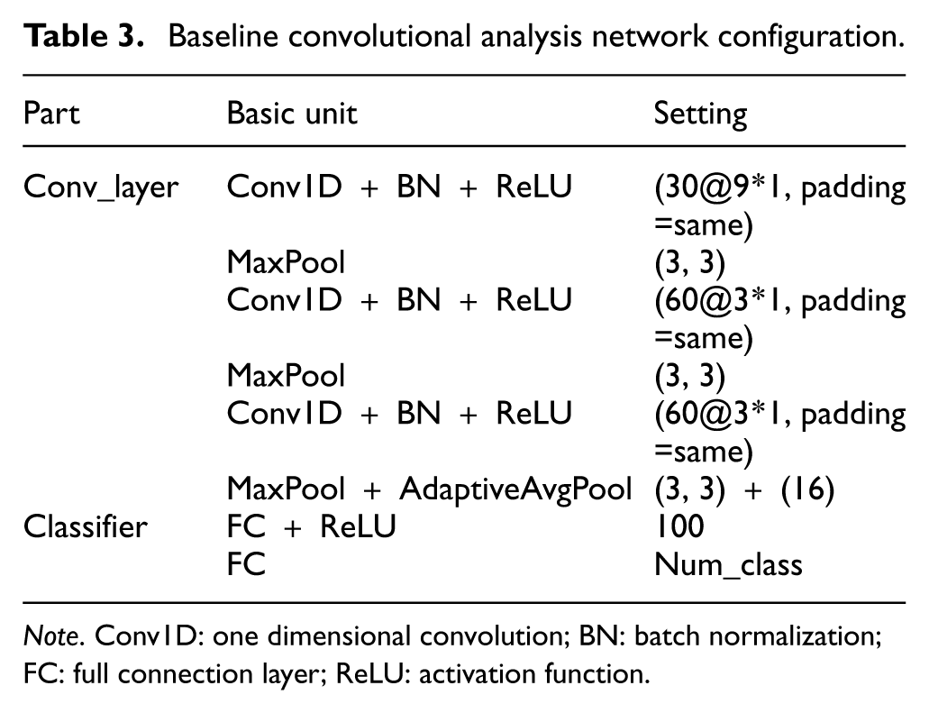
Note. Conv1D: one dimensional convolution; BN: batch normalization; FC: full connection layer; ReLU: activation function.

Testing results and analysis under noisy conditions

Test accuracy under noise scenarios is presented in Table 4, and corresponding F1-scores are shown in Figure 7. Unknown noise in test data causes feature ambiguity, significantly degrading model performance. Accuracy generally decreases as noise intensity increases in the target domain. RAOGB and HUST datasets exhibit higher noise sensitivity than BJTU and RAOMO.

Table 4.

Accuracy test results under noise scenarios.

Dataset	Var-noise task	FIE	AFIEM	AFIEF	SINC	LAPLACE	MORLET	TFN	WIL	ENVE	FREQ	FIEMIX
RAOGB	20/10 dB	91.3	74.8	81.0	46.9	56.3	49.5	51.2	50.0	70.0	51.7	89.4
	20/2 dB	60.4	52.5	51.5	31.5	34.2	26.4	29.3	20.0	22.1	20.0	58.6
	20/0 dB	50.6	49.7	42.8	27.1	26.1	20.5	27.7	20.0	20.8	20.0	53.6
	20/−2 dB	45.1	46.9	40.5	26.4	24.4	20.0	22.7	20.0	20.0	20.0	48.8
HUST	20/10 dB	94.6	93.1	88.2	44.7	44.8	45.0	45.9	84.0	72.3	81.4	94.0
	20/2 dB	65.9	65.8	55.8	25.0	25.0	25.0	25.0	60.3	52.1	38.6	64.3
	20/0 dB	55.1	57.4	48.5	25.0	25.0	25.0	25.0	31.8	43.3	34.5	55.2
	20/−2 dB	49.1	50.0	42.1	25.0	25.0	25.0	25.0	30.9	30.9	28.3	47.3
BJTU	20/10 dB	100.0	100.0	100.0	31.8	66.4	50.9	47.7	98.2	96.9	100.0	100.0
	20/2 dB	100.0	97.3	94.0	25.0	25.0	25.0	33.3	89.8	53.8	80.0	98.7
	20/0 dB	99.4	94.6	89.9	25.0	25.0	25.0	25.0	70.8	39.4	70.1	95.5
	20/−2 dB	94.5	93.3	85.9	25.0	25.0	25.0	25.0	59.0	32.0	55.4	93.3
RAOMO	20/10 dB	100.0	100.0	100.0	59.6	83.3	84.7	66.4	100.0	99.3	100.0	100.0
	20/2 dB	100.0	93.2	100.0	20.0	39.2	22.9	22.0	52.6	52.7	95.9	97.1
	20/0 dB	96.5	93.6	99.0	20.0	25.1	20.0	20.0	29.3	40.7	90.7	96.4
	20/−2 dB	96.1	88.3	95.1	20.0	24.9	20.0	21.1	20.0	23.7	86.1	93.0
AVE	20/10 dB	96.5	92.0	92.3	45.8	62.7	57.5	52.8	83.1	84.6	83.3	95.6
	20/2 dB	81.6	77.2	75.3	25.4	30.9	24.8	27.4	55.7	45.2	58.6	79.7
	20/0 dB	75.4	73.8	70.1	24.3	25.3	22.6	24.4	38.0	36.1	53.8	75.2
	20/−2 dB	71.2	69.6	65.9	24.1	24.8	22.5	23.5	32.5	26.7	47.5	70.6

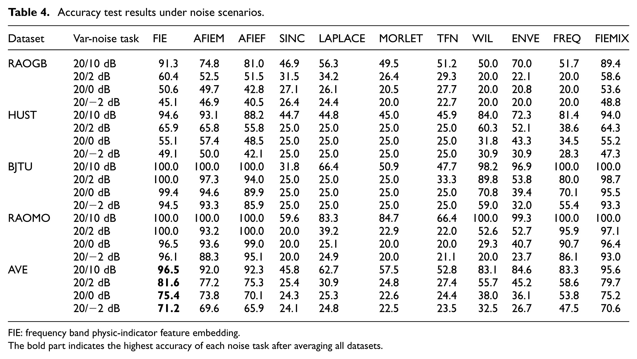
FIE: frequency band physic-indicator feature embedding.

The bold part indicates the highest accuracy of each noise task after averaging all datasets.

Figure 7.

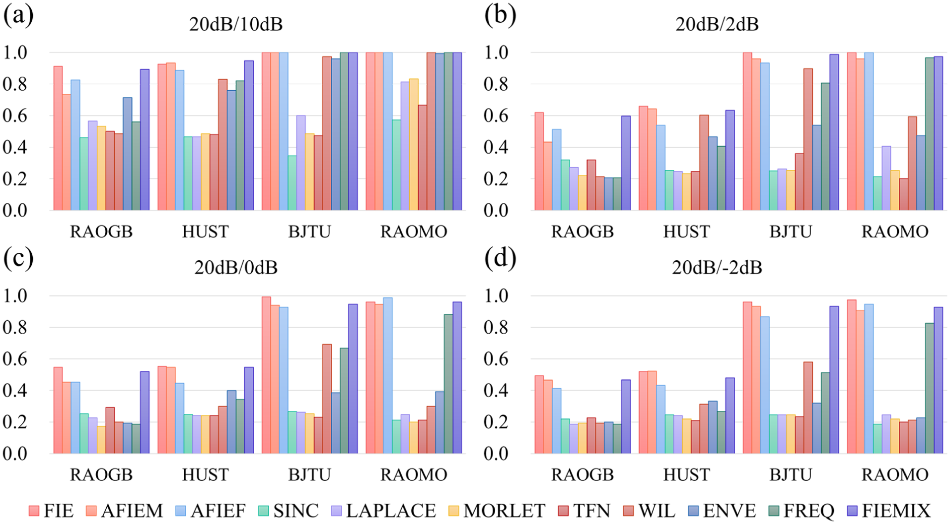
F1-score test results under noise scenarios. Where (a) to (d) represent four var-noise task codes.

Even in the 20/10 dB task with lighter noise in the target domain, methods such as TFN based on function embedding can only maintain an accuracy of about 50%, indicating that unknown noise can significantly interfere with embedding methods. The spectral simulation methods ENVE and FREQ have a relative accuracy advantage of at least 10%, proving that spectral simulation can carry more obvious fault features and has better noise resistance than function embedding methods. It is worth noting that the kernel initialized WIL method only has a performance disadvantage of 6 and 10% relative to the FIE method in the 20/2 dB task of the HUST and BJTU datasets, reflecting a certain resistance of this method to the noise environment. The FIE method can maintain an accuracy of more than 90% in the 20/10 dB task, which has a clear advantage.

In the 20/0 and 20/−2 dB tasks, the accuracy of all the comparison methods in the RAOGB and HUST datasets is only about 20% and 25%, which is on the verge of failure. In the BJTU dataset, only the WIL and FREQ methods can maintain an accuracy of more than 50%. However, FIE and its variants can still maintain a diagnostic performance of about 50% in the RAOGB and HUST datasets, and the accuracy is more than 90% in the BJTU and RAOMO datasets, which effectively proves the noise resistance of the proposed method. The FREQ method is lower than the FIE method in the 20/−2 dB task, which proves the significant advantage of the proposed method in noise resistance compared with a single spectrum.

The accuracy of each test of FIEMIX is similar to that of FIE, which verifies the applicability of FIE to the convolution variant structure. The test results of AFIEF show that the use of analog spectrum can obtain an average 5% accuracy improvement in noisy scenes and maintain better stability. The results of AFIEM show that adding weight mask can obtain an average performance improvement of about 2 and 3%, indicating that the weight mask has a certain optimization effect on noisy scenes.

The superior performance of the FIE method is attributed to structural robustness, discriminative dependency modeling, and physically guided feature constraints. First, the continuous band embedding mechanism converts discrete spectral responses into smooth statistical trends across adjacent bands. Such continuity enhances robustness to local perturbations, as noise-induced distortions typically influence isolated frequency components rather than globally dependent structures.

Second, the class-aware masking mechanism enforces discriminative dependency distributions among frequency-domain indices. Reliance on individual spectral peaks is avoided, and structured importance patterns are learned instead. This structural discrimination reduces sensitivity to noise-induced spectral fluctuations. Moreover, because the embedded indices possess explicit physical semantics, the learned feature space is constrained to a physically meaningful subspace. Consequently, physical features that are insensitive to noise variations across multiple indices can be identified more effectively, thereby mitigating overfitting and improving generalization.

Testing results and analysis under var-speed conditions

The classification accuracy under variable-speed conditions is presented in Table 5, and the F1-scores are illustrated in Figure 8. FIE is the method with the highest cumulative F1-score on each dataset. FIE leads by at least 5% in accuracy on the LV task of all datasets, and has a clear advantage in both SV and LV tasks on the HUST and BJTU datasets. This proves that the proposed method has unique advantages in cross-speed scenarios, especially in scenarios with large speed differences.

Table 5.

Accuracy test results in variable speed scenarios.

Dataset	Var-speed task	FIE	AFIEM	AFIEF	SINC	LAPLACE	MORLET	TFN	WIL	ENVE	FREQ	FIEMIX
RAOGB	NV	99.1	98.6	96.2	97.5	98.2	95.9	97.1	97.2	92.9	98.7	98.8
	SV	82.8	79.1	79.1	80.9	82.1	79.8	80.7	79.1	77.0	83.2	82.1
	LV	70.1	64.4	55.6	64.8	65.4	56.6	61.6	65.5	50	60.5	68.6
HUST	NV	99.9	99.7	99.8	99.9	99.8	99.7	100.0	99.2	97.6	99.8	99.8
	SV	85.4	88.0	80.4	67.6	60.1	59.1	60.2	54.8	60.7	72.2	83.3
	LV	70.4	67.0	55.4	50.2	48.4	48.3	50.5	45.7	59.5	56.0	73.0
BJTU	NV	100.0	100.0	100.0	100.0	100.0	100.0	100.0	100.0	100.0	100.0	100
	SV	88.7	89.0	86.1	85.5	80.7	77.1	84.6	78.8	74.7	81.1	87.4
	LV	78.9	76.6	76.1	73.6	58.6	57.5	71.7	62.3	48.6	70.9	76.7
RAOMO	NV	100.0	100.0	100.0	100.0	100.0	100.0	100.0	100.0	100.0	100.0	100.0
	SV	68.6	64.9	68.3	64.5	55.9	49.6	60.8	68.8	62.5	63.4	73.1
	LV	43.3	42.1	42.7	29.9	31.9	22.8	38.2	37.5	40.5	39.9	46.0
AVE	NV	99.8	99.6	99.0	99.4	99.5	98.9	99.3	99.1	97.6	99.6	99.7
	SV	81.4	80.3	78.5	74.6	69.7	66.4	71.6	70.3	68.7	75.0	81.5
	LV	65.7	62.5	57.5	54.6	51.1	46.3	55.5	52.8	49.7	56.8	66.1

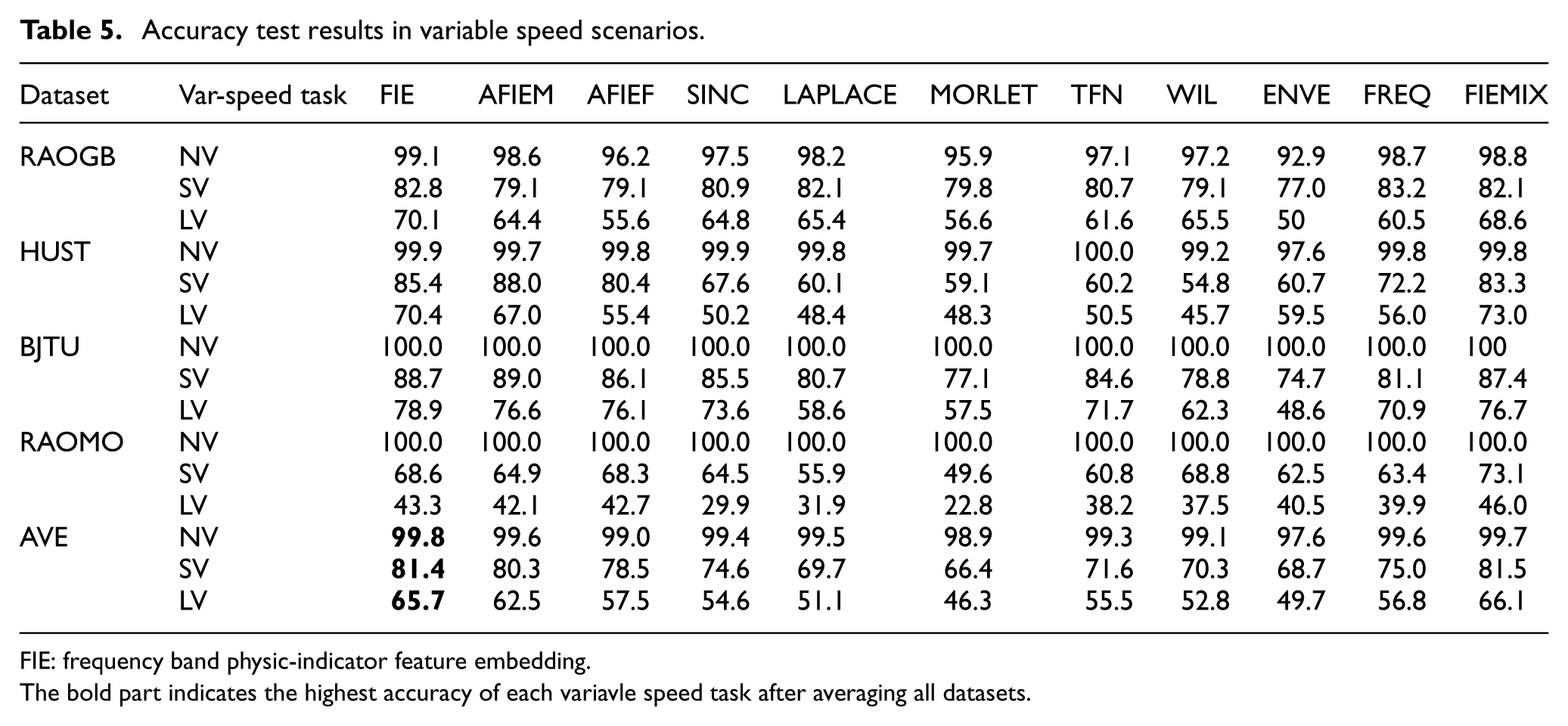
FIE: frequency band physic-indicator feature embedding.

The bold part indicates the highest accuracy of each variavle speed task after averaging all datasets.

Figure 8.

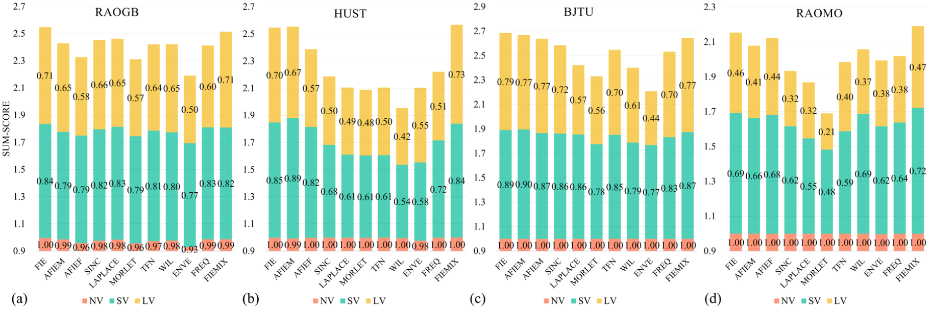
F1-score test results in variable speed scenarios. Where (a) to (d) represent var-speed task codes on four datasets.

Kernel function embedding methods exhibit inferior performance, especially in LV tasks. The TFN and SINC methods yield average LV accuracies 10% lower than FIE. The Morlet method performs worse than that of TFN and SINC, with a gap of 10% in the SV scenario and 15% in the LV scenario on the BJTU and RAOMO datasets. This performance degradation of kernel function embedding methods may result from significant time-domain feature shifts induced by speed variations.

The kernel-initialized comparison model WIL is only 5% lower than the FIE method in the LV task of the RAOGB and RAOMO datasets. However, it has a gap of 20 and 10% in the HUST and BJTU datasets, respectively. Considering that the RAOGB and RAOMO datasets are collected from the same platform, the WIL method may be more suitable for datasets carrying certain types of features, but this also shows that its stability is not good.

The spectrum simulation ENVE method has only about 50% accuracy in the LV task of the RAOGB and BJTU datasets. This may be because the speed change will have a greater impact on the position of the fault spectrum. The performance of the FREQ method in each dataset is relatively high among the comparison methods, which means that the spectrum can carry more domain-invariant features in cross-speed scenarios. However, due to the insufficient amount of features carried by a single channel, it is 6 and 9% lower than the FIE method on average in the SV and LV tasks.

AFIEF is 7% lower than FIE in LV tasks, indicating that spectrum simulation improves robustness under speed variation. The test results of AFIEM show that the use of weight mask can slightly improve the diagnostic accuracy by about 2%, which helps the subsequent feature analysis process. FIEMIX exhibits comparable performance to the backbone network, demonstrating that FIE can be effectively integrated into various convolutional architectures.

A high-density continuous band filter bank is constructed in FIE, allowing frequency-domain indices to form smoothly varying statistical trends along the frequency axis. Class discrimination is thus encouraged to depend on structural patterns rather than single-frequency responses. Model decisions are based not only on the magnitude of the original feature values but also on whether the current sample exhibits an index dependency structure consistent with a certain class. When rotational speed changes, even if a single-frequency band feature is disturbed, as long as the overall dependency structure maintains its discriminative power, model performance will not drastically decline. Model decisions are determined not only by feature magnitudes but also by the consistency of the sample’s index dependency structure with a specific class. Even if individual band features are perturbed under rotational speed variation, performance degradation is avoided as long as the global dependency structure remains discriminative.

Frequency-domain statistical indices possess clear physical interpretations and exhibit greater stability across rotational speed conditions than purely data-driven features. The learning space is therefore restricted to a semantically meaningful subspace. This structural constraint reduces dependence on incidental data patterns and enhances cross-condition generalization. Experimental results confirm the effectiveness of the framework design implemented in the FIE module.

Discussion

Parameter sensitivity analysis

A parameter sensitivity analysis was performed on four datasets under var-speed and two cross-noise scenarios (20/2 and 20/−2 dB) for the FIE module. Involving the number of filter banks, filter order, and sliding window size. The hyperparameter grid was: number of filter banks [200, 400, 600, 800], filter order [400, 800, 1000, 1200, 1600], and sliding window size [9, 15, 32, 48]. Given that the size and order of the filter bank directly affect the computational complexity of the model, a lightweight configuration sensitivity analysis was performed using a step-decreasing number and order of filters. Five step-decreasing filter bank configurations were designed: [600 × 1000, 500 × 800, 400 × 600, 300 × 400, 200 × 200].

Figure 9 presents sensitivity results across datasets. Different datasets exhibited distinct sensitivities: BJTU was most sensitive, whereas RAOMO was least. Sensitivity also differed by task, with RAOGB and HUST showing higher sensitivity in cross-noise tests, and BJTU and RAOMO being more affected in var-speed tests.

Figure 9.

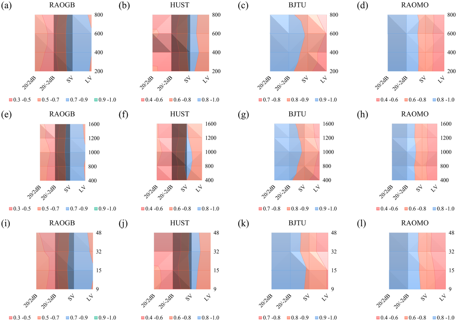
Parameter sensitivity test results, the top row (a–d) is the number of filters experiment results in each dateset, the middle row (e–h) is the filter order experiment results in each dateset, and the bottom row (i–l) is the sliding window sizeexperiment results in each dateset.

The number of filters determines spectral sampling density. An insufficient number (e.g., 200) yields sparse frequency coverage, enlarges inter-band intervals, and prevents formation of a continuous spectral trend, thereby weakening the structural representation of the perceptual mask along the frequency axis and inducing information loss. Increasing the number to 800 enhances spectral resolution but introduces redundant details. On the BJTU dataset, excessively high resolution may amplify local perturbations, slightly dispersing structure-dependent patterns and causing minor performance degradation.

Filter order governs frequency selectivity sharpness. A low order captures only coarse spectral trends and fails to represent subtle modulation features in variable-speed tasks (HUST and BJTU). An excessively high order produces over-selectivity, potentially preserving substantial high-frequency noise and reducing robustness in cross-noise tests (such as RAOGB).The sliding window size reflects trend smoothness. Larger windows produced overly coarse trends, reducing diagnostic accuracy on BJTU and HUST. A window size of 15 offered satisfactory results, as smaller divisions provided little improvement but higher computational complexity.

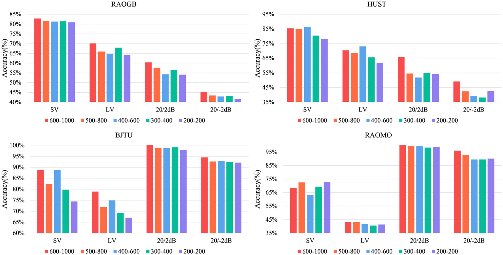
The results of the sensitivity experiment of lightweight filter bank configuration are shown in the Figure 10. When the number of filters and the order of filters are reduced at the same time, the model performance will gradually decrease in most scenarios, but there will be no sudden collapse. Certain medium-scale configurations demonstrate superior performance; for instance, the configuration (400 filters, 600th order) performs remarkably on the HUST and BJTU datasets. Under smaller configurations, performance decreases noticeably, yet acceptable diagnostic capability is retained.

Figure 10.

Sensitivity experiment of lightweight configuration of filter bank parameters.

The number of filters controls frequency sampling density of the simulated spectrum, whereas filter order determines selectivity sharpness and bandwidth resolution. When both decrease, frequency partitioning becomes coarser, continuous trend representation weakens, frequency leakage intensifies, local statistical characteristics become blurred, and stability of the feature distribution underlying the class-aware weight mask is reduced. Nevertheless, experimental results confirm that acceptable diagnostic performance is preserved under lower configurations.

These findings indicate that effectiveness of the FIE method does not rely on ultra-high-resolution settings, and the continuous frequency band embedding mechanism maintains structural stability over a broad parameter range. In practical deployment, FIE can be configured according to scenario requirements, exhibiting favorable complexity–performance trade-offs. A stable high-performance parameter region is observed rather than a single-point optimum. Performance variation correlates with spectral structural expressiveness, and degradation induced by parameter reduction arises from gradual sparsification of the continuous band structure rather than structural failure. Robustness to parameter variation is therefore demonstrated.

Figure 11 compares the average computational efficiency of different methods per sample over one epoch. Although the FIE module requires extra computation for analog spectrum generation and feature segmentation, its training speed remained comparable to other methods and faster than TFN and ENVE method. This is because although it has more operation steps, its calculation process is not complicated. Despite slightly longer testing time, its per-sample latency stayed within the millisecond range, meeting diagnostic requirements. Ablation results confirmed that analog spectra-based achieved better performance than FFT-based spectra across datasets. Considering both its diagnostic effectiveness and interpretability in decision reliability, the computational of FIE module was acceptable.

Figure 11.

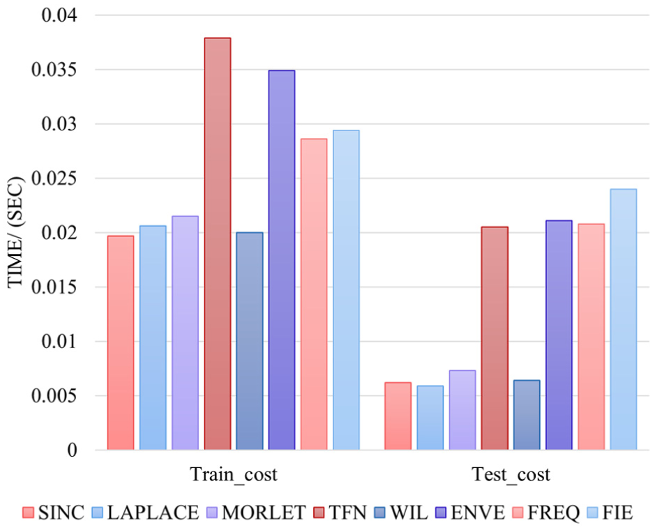
Comparison of training and testing time of each method.

Degradation behavior analysis of class-aware weight mask under noise

To systematically evaluate the stability of frequency-domain indicators under varying noise intensities, class-aware weight mask trend graphs were generated for the RAOGB and HUST datasets at different noise levels (20 dB, 2 dB, −2 dB), as illustrated in Figure 12. Comparison of the mask distributions across signal-to-noise ratios reveals pronounced differences in spectral characteristics of health states and fault types between datasets. Moreover, the “primary discrimination frequency domain indicators” automatically learned on different datasets are inconsistent. Hence, the key frequency bands and statistical indicators utilized for discrimination are determined by dataset characteristics rather than category attributes.

Figure 12.

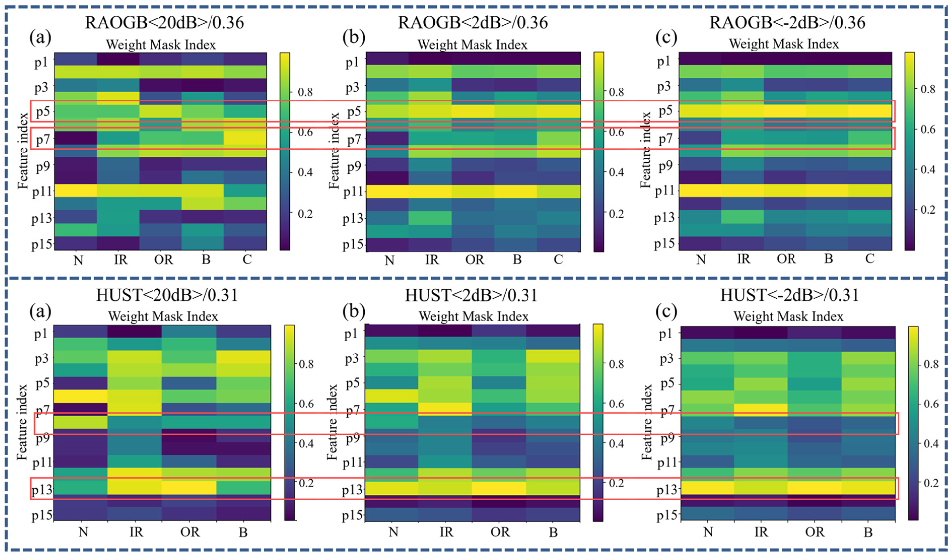
Trend chart of class-aware weight mask variation under different noise intensities. Where (a–c) represents different experiment noise condition codes.

As shown in the figure, under low-noise conditions, class-aware weight masks preserve clear discriminative structures, with distinct weight distributions across categories in the frequency-band indicator space. With increasing noise intensity, interclass differences in weight distribution are markedly reduced, exhibiting a convergence phenomenon, and frequency-band indicators that originally displayed significant responses become progressively smoothed. In particular, within the frequency-domain index region highlighted by the red box, frequency bands with initially significant interclass weight differences demonstrate pronounced convergence under extreme noise. This observation indicates that noise perturbation attenuates the discriminative contribution of these frequency-domain indices, submerges their statistical characteristics in random noise, and disrupts the original spectral structure through high-frequency stochastic disturbances.

Under extreme noise conditions, the expressive capacity of the class-aware weight mask is consequently degraded. When clear structural separation among class masks cannot be maintained, overall diagnostic performance declines. This phenomenon further supports the proposed mechanism, as model performance is shown to be strongly correlated with the stability of the class mask structure: When the structural differences are clear, the diagnostic performance is stable; when the structure becomes blurred and convergent, the diagnostic performance declines accordingly.

Class-aware weight mask behavior analysis

Most existing preanalysis modules can only demonstrate self-interpretability, without revealing the key features on which decisions depend and assessing decision credibility. The class-aware weight mask in FIE partially addresses these limitations.

The distance matrix is derived by computing the average distance (via Equation (20)) between the weight mask of each test sample and the center distribution of each class mask. The [i, j]th element indicates the average distance between samples of class i and the class j mask center. As observed in Figure 11, test samples exhibit strong alignment with the indicator distribution of their true class, while the distances to other classes remain distinct. These weight masks serve as key features on which model decisions depend. By measuring the distance to each class center, the correspondence between selected indicators and fault-specific patterns can be assessed. In this article, the thresholds calculated for each dataset are as follows: (RAOGB: 0.36, HUST: 0.31, BJTU: 0.58, RAOMO: 0.42).

DIS [i, j] = \frac{1}{N} \sum_{t = 1}^{N \in i} Sim [j]

(20)

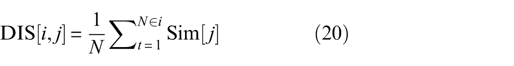
When the relationship between the distance matrices derived from the test signal and the threshold of the current dataset does not satisfy the criterion described in “Decision reliability judgment mechanism based on class-aware weight mask” section, it indicates that the weight distribution of the selected indicator fails to match the central physical feature distribution of any category, implying reduced decision confidence. The weight mask also provides a reference for analyzing model failure. Figure 13 presents the t-SNE (t-Distributed Stochastic Neighbor Embedding) visualization of the confusion matrix, weight mask distribution, and distance metric matrix under different tasks. The red circles denote the weight mask distribution of a target-domain category and its corresponding source-domain distribution, the yellow circles denote misclassified source-domain categories, and the blue circles denote weight mask distributions below the threshold in the cross-noise task.

Figure 13.

Each column represents a different experiment: (a–d) t-SNE results of source domain training and target domain test samples weight mask, (e–h) confusion matrix of the test task, and (i–l) Euclidean distance matrix of the test task.

For example, in the confusion matrix of RAOGB, when inner ring fault signals are misclassified as healthy, the weight mask distribution generated by the target domain inner ring fault signals are positioned near the healthy-state signal in the source domain, which may interfere with subsequent analysis modules. The clustering results within the blue circle on the BJTU and RAOMO datasets show that weight masks below the threshold are closely grouped, indicating higher decision confidence.

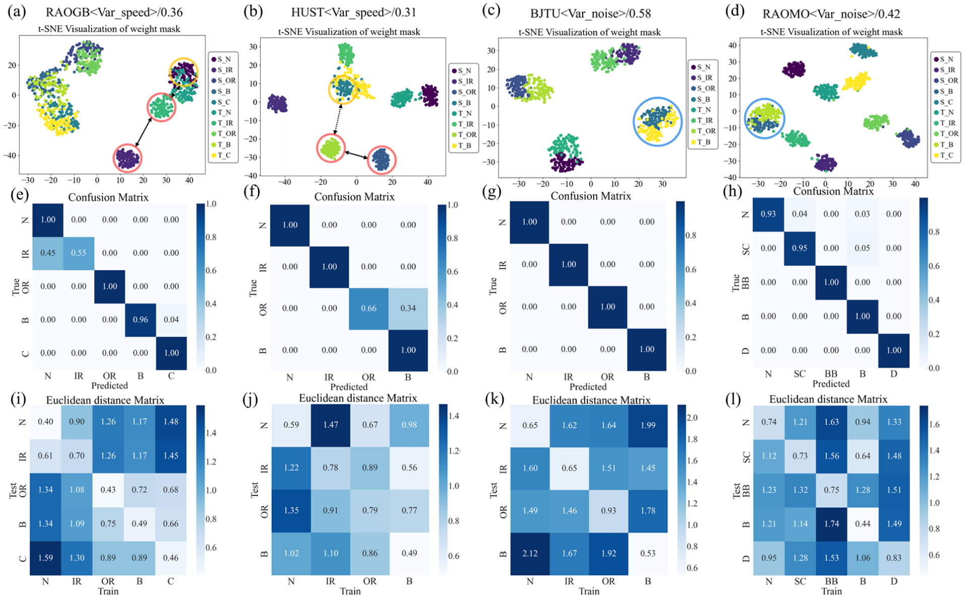
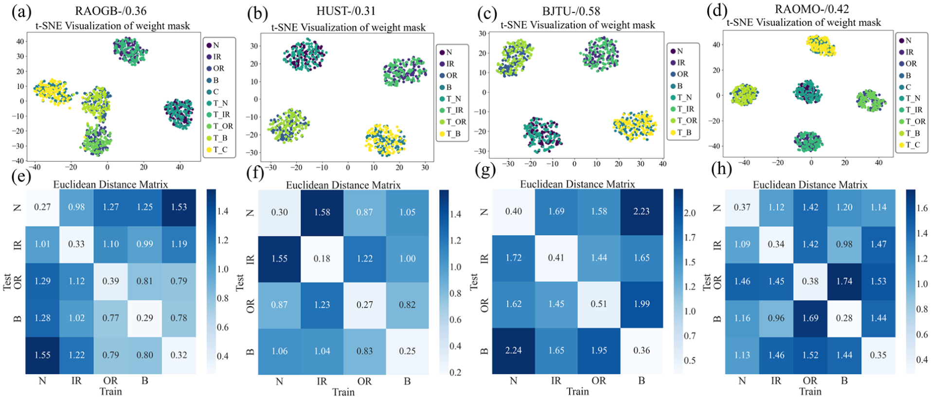
Figure 14 illustrates the distance matrix behavior during source-domain testing, whereas Figure 15 shows the corresponding behavior under varying noise levels, speeds, and datasets in cross-domain tasks. The following observations are obtained: (1) In source-domain testing, the distance between the test mask and a specific class center is markedly smaller than that to other class centers and remains below the effective threshold. Since a weight distribution highly consistent with class-specific fault indicators is obtained, and high decision confidence is indicated. (2) In cross-domain tasks, feature drift prevents distances from falling below the threshold. When the distance to one class center is smaller than that to other classes by at least an effective threshold, the selected indicator is considered more consistent with that class, and high decision confidence is maintained (with an accuracy of over 90%), as observed in the health status and inner circle fault identification of the 2 dB task in the RAOGB dataset. (3) Even when the distances to all class centers fail to satisfy the two constraints in “Decision reliability judgment mechanism based on class-aware weight mask” section and remain similar across classes, resulting in low confidence, correct classification may still be achieved because the final decision is produced by the subsequent analysis network based on interpreted features. For example, in the outer circle fault diagnosis of the A–C cross-condition task in the BJTU dataset, correct decisions are obtained despite low confidence. Therefore, it is important to emphasize that poor decision credibility does not necessarily mean that the decision is wrong.

Figure 14.

Each column represents a different experiment: (a–d) classification results of source domain training and test samples weight mask, and (e–h) Euclidean distance matrix of the test samples.

Figure 15.

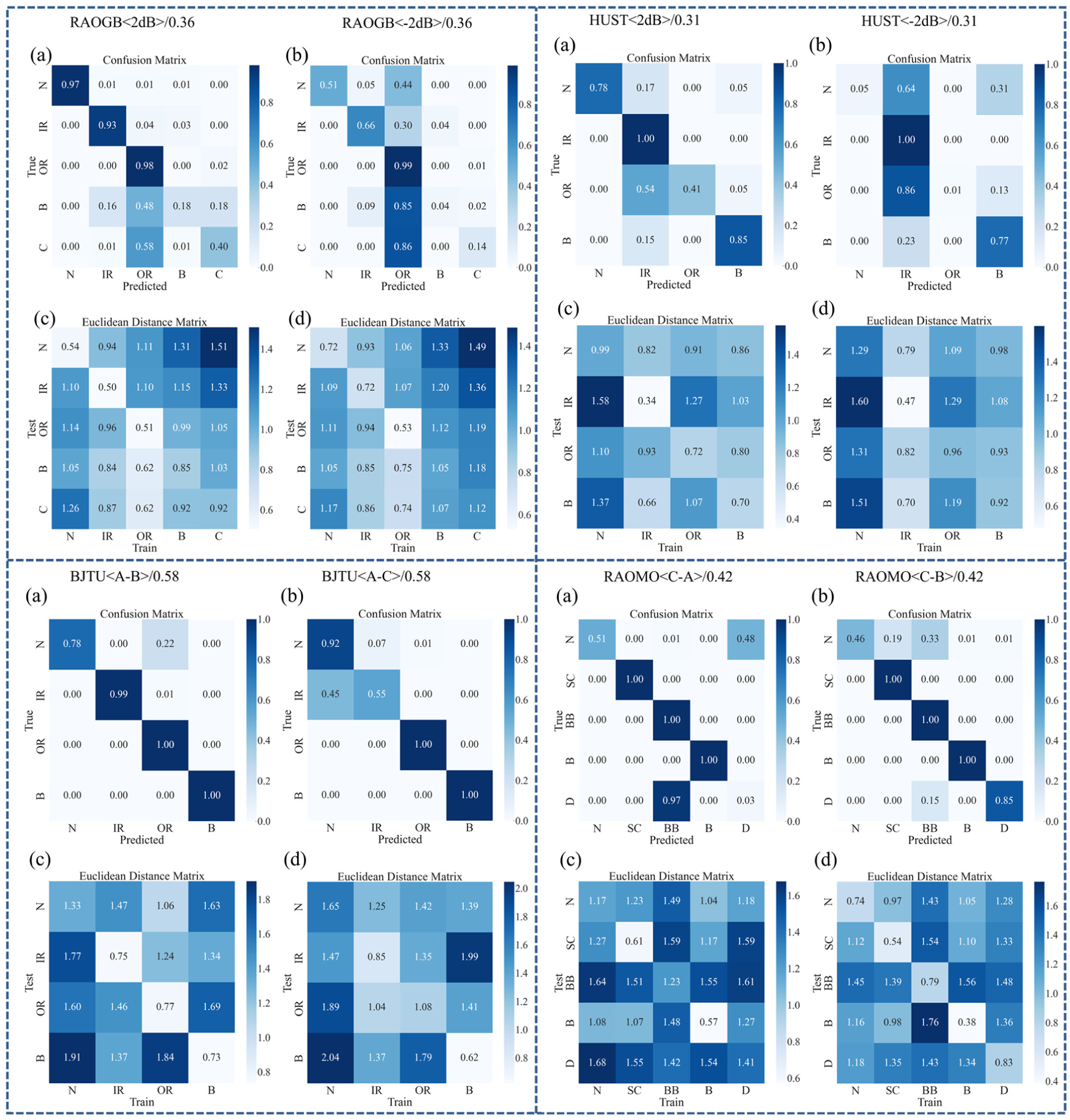
Each blue box in the figure represents the visualization result of a dataset: (a and b) in each box represents the cross-domain test task confusion matrix and (c and d) in each box represents the corresponding distance matrix for the test task.

Existing fault diagnosis approaches related to interpretability or decision confidence can be categorized into post hoc interpretation, uncertainty quantification, and prototype-based learning. Post hoc methods are imposed on a fixed decision function, and their interpretability is descriptive. In contrast, the FIE module embeds physically meaningful frequency-domain indicators into feature construction. Class-aware weight masks and classifiers are jointly optimized via triplet loss, such that interpretable variables directly participate in decision boundary formation. Consequently, interpretability in FIE is intrinsic and structurally constrained.

Uncertainty quantification methods evaluate probabilistic instability rather than feature-level inconsistency. In contrast, confidence assessment based on class-aware weight masks originates from the consistency of class-specific indicator weight distributions. The distance between a test mask and a class center reflects structural consistency with learned importance patterns of fault-related features. Prototype-based methods typically learn abstract high-dimensional representations, whereas class centers obtained by FIE correspond to identifiable frequency-domain feature patterns with explicit physical meaning.

Based on the above analyses and comparisons, the FIE framework integrates physical embedding, discriminative weighting, and reliability assessment within a unified structural design. A self-interpretive diagnostic paradigm grounded in physical space is thereby established, distinguishing it from existing interpretability approaches.

Conclusion

To address the limitations of neural networks in high-reliability scenarios due to poor interpretability and low confidence, a self-interpretable frequency band physic-indicator FIE module is proposed. This module extracts continuously varying multichannel regional frequency features using multiple frequency-domain statistical indicators derived from the analog spectrum. A class-aware weight mask is subsequently generated to weight each feature channel, enabling its use both as a key factor in classification decisions and for evaluating decision credibility. The proposed FIE module surpasses baseline models by at least 12% under various noise conditions, and by 6 and 9% in the SV and LV scenarios, respectively. It enhances overall diagnostic performance and is adaptable to various network architectures. Visualization of the weight distribution distance confirms that the class-aware weight mask provides analyzable indicator features for decision analysis and facilitates decision credibility assessment through distance-based evaluation. Future work will focus on extending the proposed framework toward decision-level interpretability while further improving generalization in practical applications. While this study established an interpretable module and proposed a method for assessing decision credibility, it has not yet achieved decision-level interpretability. Future research will focus on decision-level interpretability to explore more in-depth interpretable diagnostic methods.

Footnotes

Declaration of conflicting interests

The authors declared no potential conflicts of interest with respect to the research, authorship, and/or publication of this article.

Funding

The authors disclosed receipt of the following financial support for the research, authorship, and/or publication of this article: This research was funded by the Fundamental Research Funds for the Central Universities (2023JBZY039), the Beijing Natural Science Foundation (grant no. L211010), and the Beijing Infrastructure Investment Research Project.

Consent to participate

This article does not contain any studies with human or animal participants.

ORCID iD

Qingbin Tong

References

Tang

Pang

. Simulation-driven unsupervised fault diagnosis of rolling bearing under time-varying speeds. Struct Health Monit 2025; 24: 3275–3291.

Park

Jang

, et al. Adaptive bearing fault diagnosis using reference frequency and modified scalogram. Struct Health Monit 2024; 23: 2781–2794.

Jia

Chow

TWS

Yuan

. Causal disentanglement domain generalization for time-series signal fault diagnosis. Neural Netw 2024; 172: 106099.

Tong

Jiang

, et al. Prior knowledge embedding convolutional autoencoder: a single-source domain generalized fault diagnosis framework under small samples. Comput Ind 2025; 164: 104169.

Huo

Jiang

, et al. An unsupervised transfer learning approach for rolling bearing fault diagnosis based on dual pseudo-label screening. Struct Health Monit 2024; 23: 2288–2309.

Men

Bai

, et al. A bearing fault diagnosis method based on M-SSCNN and M-LR attention mechanism. Struct Health Monit 2025; 24: 830–852.

Meng

, et al. Intelligent fault diagnosis of high-speed train axle box bearings under parameter fluctuation working conditions using continuous cohomology-based meta-transfer learning framework. Struct Health Monit 2026; 25: 393–412.

Zhao

Shen

. A domain generalization network combing invariance and specificity towards real-time intelligent fault diagnosis. Mech Syst Signal Process 2022; 173: 108990.

Jia

Chow

TWS

Wang

, et al. Dynamic balanced dual prototypical domain generalization for cross-machine fault diagnosis. IEEE Trans Instrum Meas 2024; 73: 1–10.

10.

Lei

Yang

Jiang

, et al. Applications of machine learning to machine fault diagnosis: a review and roadmap. Mech Syst Signal Process 2020; 138: 106587.

11.

Tong

Jiang

, et al. Adaptive single-source open domain generalization network: a novel physical information fusion framework for fault diagnosis based on physically embedded autoencoder and adaptive open-set feature separation. Adv Eng Inform 2025; 68: 103632.

12.

Wang

Zhou

. Key-performance-indicator-related process monitoring based on improved kernel partial least squares. IEEE Trans Ind Electron 2021; 68: 2626–2636.

13.

Chen

H-Y

Lee

C-H

. Vibration signals analysis by explainable artificial intelligence (xai) approach: application on bearing faults diagnosis. IEEE Access 2020; 8: 134246–134256.

14.

Chen

Liu

. A novel convolutional neural network with global perception for bearing fault diagnosis. Eng Appl Artif Intell 2025; 143: 109986.

15.

Qin

Zhang

Qian

, et al. Large model for rotating machine fault diagnosis based on a dense connection network with depthwise separable convolution. IEEE Trans Instrum Meas 2024; 73: 1–12.

16.

Liu

Chen

, et al. MPNet: a lightweight fault diagnosis network for rotating machinery. Measurement 2025; 239: 115498.

17.

Sun

Yan

Jin

, et al. LiteFormer: a lightweight and efficient transformer for rotating machine fault diagnosis. IEEE Trans Reliab 2024; 73: 1258–1269.

18.

Jiao

Pan

Fan

, et al. Partly interpretable transformer through binary arborescent filter for intelligent bearing fault diagnosis. Measurement 2022; 203: 111950.

19.

Shang

Zhao

Yan

. Denoising fault-aware wavelet network: a signal processing informed neural network for fault diagnosis. Chin J Mech Eng 2023; 36: 9.

20.

Tong

Jiang

, et al. Wavelet packet energy embedded autoencoder with dynamic weighting strategy for fault diagnosis under unknown working conditions. Reliab Eng Syst Saf 2026; 265: 111528.

21.

Xie

Wang

, et al. Sparse sample train axle bearing fault diagnosis: a semi-supervised model based on prior knowledge embedding. IEEE Trans Instrum Meas 2023; 72: 1–11.

22.

Wang

Han

Liu

, et al. A globally interpretable convolutional neural network combining bearing semantics for bearing fault diagnosis. IEEE Trans Instrum Meas 2025; 74: 1–13.

23.

Liu

Ding

, et al. An interpretable multiplication-convolution network for equipment intelligent edge diagnosis. IEEE Trans Syst Man Cybern Syst 2024; 54: 3284–3295.

24.

Shi

, et al. Physics-informed interpretable wavelet weight initialization and balanced dynamic adaptive threshold for intelligent fault diagnosis of rolling bearings. J Manuf Syst 2023; 70: 579–592.

25.

Shi

Liu

, et al. Interpretable physics-informed domain adaptation paradigm for cross-machine transfer diagnosis. Knowl Based Syst 2024; 288: 111499.

26.

Tong

Jiang

, et al. Envelope spectrum neural network with adaptive domain weight harmonization for intelligent bearing fault diagnosis under cross-machine scenarios. Adv Eng Inform 2024; 62: 102787.

27.

Grezmak

Zhang

Wang

, et al. Interpretable convolutional neural network through layer-wise relevance propagation for machine fault diagnosis. IEEE Sens J 2020; 20: 3172–3181.

28.

Sanakkayala

Varadarajan

Kumar

, et al. Explainable AI for bearing fault prognosis using deep learning techniques. Micromachines 2022; 13: 1471.

29.

Shen

Wei

Huang

, et al. Interpretable compositional convolutional neural networks. Proc Int Joint Conf Artif Intell (IJCAI) 2021; 2971–2978.

30.

Ravanelli

Bengio

. Interpretable convolutional filters with SincNet. arXiv 2018; abs/1811.09725.

31.

Zhu

Liu

Bao

, et al. Decoupled interpretable robust domain generalization networks: a fault diagnosis approach across bearings, working conditions, and artificial-to-real scenarios. Adv Eng Inform 2024; 61: 102445.

32.

Sun

, et al. WPConvNet: an interpretable wavelet packet kernel-constrained convolutional network for noise-robust fault diagnosis. IEEE Trans Neural Netw Learn Syst 2024; 35: 14974–14988.

33.

Feng

Zheng

Chen

, et al. Beyond deep features: fast random wavelet kernel convolution for weak-fault feature extraction of rotating machinery. Mech Syst Signal Process 2025; 224: 112057.

34.

Chen

Dong

, et al. TFN: an interpretable neural network with time-frequency transform embedded for intelligent fault diagnosis. Mech Syst Signal Process 2024; 207: 110952.

35.

Ding

Qin

Wang

, et al. Evolvable graph neural network for system-level incremental fault diagnosis of train transmission systems. Mech Syst Signal Process 2024; 210: 111175.

36.

Zhao

Zio

Shen

. Domain generalization for cross-domain fault diagnosis: an application-oriented perspective and a benchmark study. Reliab Eng Syst Saf 2024; 245: 109964.

37.

Zhao

Sun

, et al. WaveletKernelNet: an interpretable deep neural network for industrial intelligent diagnosis. IEEE Trans Syst Man Cybern Syst 2022; 52: 2302–2312.

38.

Farag

. Design and analysis of convolutional neural layers: a signal processing perspective. IEEE Access 2023; 11: 27641–27661.

39.

Zhao

Jiao

. A Fault diagnosis method for rotating machinery based on CNN with mixed information. IEEE Trans Ind Inform 2023; 19: 9091–9101.