Damage identification and level evolution probabilistic risk assessment of corroded reinforced concrete beams using multi-domain dynamic and static data with deep learning

Abstract

The dynamic response of post-fire corroded concrete structures under time-varying loads continues to evolve, resulting in the progressive development of damage levels. However, existing standards often fail to fully account for this entire process. To investigate the evolution of damage levels in structures, this study proposes a framework that integrates finite element models (FEMs) with deep learning for damage identification and probabilistic risk assessment. The method first utilizes multi-domain experimental data, including dynamic and static responses, to correct the physical parameters of the initial FEM via residual network. Based on the updated high-precision model, the static reduction coefficients can be effectively predicted with an error controlled within 5%. Furthermore, by combining the static reduction coefficients with multi-domain dynamic information, the multi-granularity spatial-temporal attention learning evaluation branch is employed to derive the damage contribution rates and the comprehensive index, multi-variable feature index (MVFI). Using the MVFI, the probability density fitting analysis based on R² is conducted to determine the optimal distribution models for different damage levels. Finally, by integrating the prior-based minimum expected loss criterion with posterior probabilities, a comprehensive assessment of damage level evolution is achieved. Compared with conventional static-load tests that provide only local, static information, the proposed multi-domain probabilistic estimation method can effectively evaluate the damage evolution throughout the service life of the structure and offers the potential for local deployment.

Keywords

MG-STAL RP-SE-ResNet-50 model update corroded reinforced concrete beam damage identification and assessment

Highlights

This study introduces a novel damage identification method using recurrence plots (RPs) and SE-ResNet50, achieving high accuracy for fire-damaged and corroded reinforced concrete beams.

The study develops an enhanced finite element model updating strategy, reducing prediction error to within 5% for damaged beam responses.

A comparative analysis is conducted between one-dimensional time-domain signals and two-dimensional RPs, showing superior performance in accuracy and convergence speed with RP data.

The dynamic evolution of damage in fire-damaged and corroded beams is assessed using multi-granularity spatial-temporal attention learning module and probability density analysis, with consistent results.

A new composite index (multi-variable feature index) is introduced for comprehensive assessment of multi-domain dynamic and static data in structural health monitoring.

Introduction

Reinforced concrete (RC) beams, owing to their excellent practicality and cost-effectiveness, have been widely used in civil infrastructure. However, among various failure modes, concrete beams often lose their load-bearing capacity due to excessive static loads or excessive flexural deformations. When structures are subjected to multiple types of damage, such as fire exposure and corrosion, their performance degradation becomes more significant, potentially leading not only to severe structural failures but also to threats to life and property.^1–4 The accumulation of local damage often results in progressive failure of concrete beams; therefore, the ability to strengthen the structure based on its dynamic and static responses as well as its damage levels before ultimate failure is critical for ensuring durability. Currently, techniques for detecting both global and local structural damage have been extensively studied, with various methods optimized for specific structural forms and damage types. Among these, vibration-based damage detection, as a global approach, employs distributed sensors to acquire synchronized structural response data. However, it exhibits limitations in capturing diverse structural responses and characterizing the evolution of structural damage. Such damage identification problems can be addressed within an inverse problem framework by updating finite element models (FEMs),⁵ that is, by inferring structural parameters from measured responses, and estimating stiffness reductions induced by damage.⁶ Most existing studies integrate computational models with parameter identification techniques to handle large sets of identification parameters.⁷ For local damage, such as cracks and spalling, research has focused on using input–output signal reciprocity to identify specific features.⁸

Vibration-based structural health monitoring has emerged as an active area of research in recent years, with widely adopted indicators including natural frequencies,^9–11 mode shapes and their derivatives,^12,13 damping ratios,^14,15 and stiffness variations. However, while such methods can effectively reduce relative errors, they remain vulnerable to absolute errors, which may stem from measurement inaccuracies, modeling errors, and differences in boundary conditions between experiments and simulations. According to the nature of these errors, they can be classified into structural, parameter, and model-order errors.^5,16

To enhance model reliability, researchers have developed various techniques for interactive model parameter updates based on experimental data and numerical simulations. For example, damage functions in RC structures have been updated,¹⁷ model update has been performed using modal flexibility residuals or frequency response functions.^18,19 Specifically, Shiradhonkar and Shrikhande¹⁹ updated the FEM of concrete beams based on vibration signals; Steinwender and Nordmann²⁰ corrected the model stiffness based on measured eigenvalues; and Shahandashti and Ashuri²¹ developed the vector error correction model method. Representative FEM-ML studies, together with their task types and main limitations, are summarized in Table 1.

Table 1.

Representative FEM-ML studies, their task types, and main limitations.

FEM-Machine learning (ML) method	Task type	Main limitation
Modal flexibility residual and Frequency Response Function (FRF)-based model updating²²	Structural model updating	Mainly linear-analysis-based; limited for nonlinear and non-stationary responses
Vibration-signal-based FEM updating¹⁹	Concrete beam model updating	Relies on conventional signal features; limited feature representation capability
Vector error correction model²¹	Structural damage identification and model correction	Focused on signal relation modeling; limited integration with probabilistic assessment
FEM and ML⁷	Damage identification and prediction	Mainly deterministic output; limited uncertainty quantification
FEM and deep learning framework⁸	Structural response prediction and assessment	Mostly task-specific; limited dynamic-static fusion and full-process probabilistic assessment

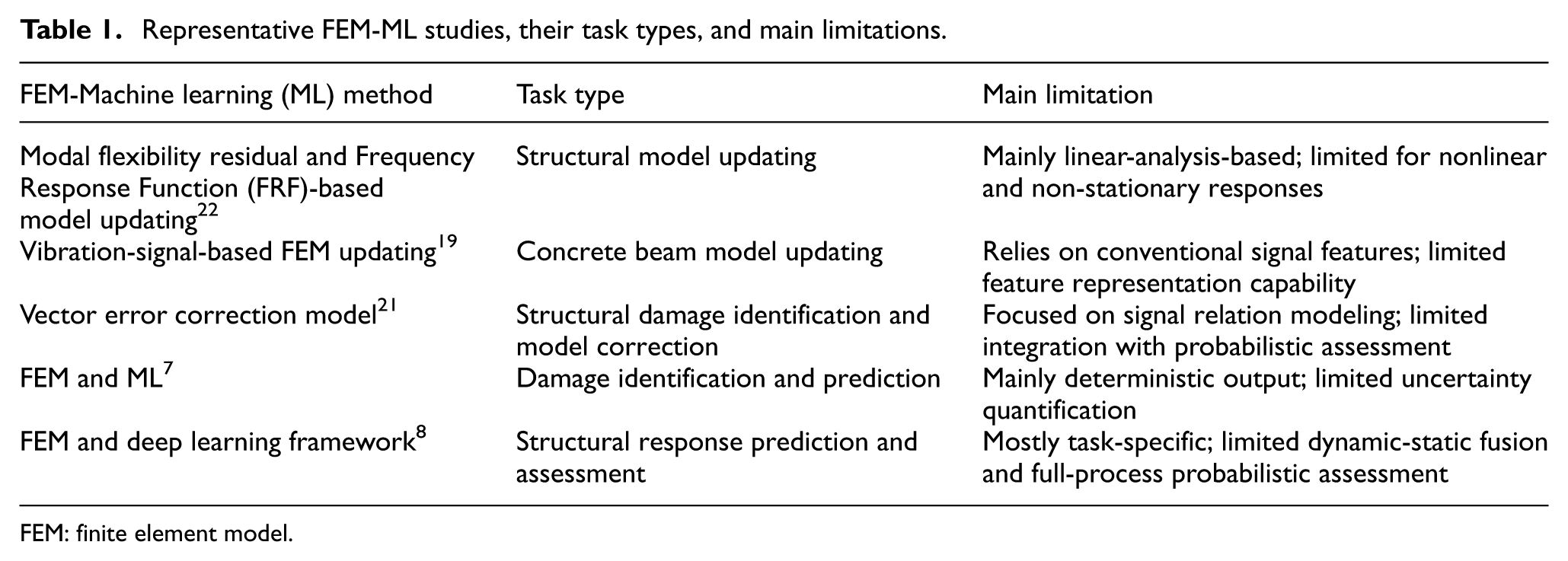
FEM: finite element model.

As shown in Table 1, existing studies have achieved encouraging progress in FEM-based structural damage analysis; however, most of them still rely on conventional signal representations and deterministic analysis frameworks. In particular, traditional linear analysis methods have significant limitations in capturing the nonlinear and time-varying characteristics of dynamic signals. To address this issue, this study introduces the recurrence plot (RP) method to store and visualize dynamic information of structural components. By reconstructing the phase space and utilizing recurrence matrix, this method transforms non-stationary time series into two-dimensional (2D) images, effectively revealing complex dynamic patterns hidden within the signals.^23,24 Numerous studies have successfully employed RP in various contexts. For example, Zhou et al.²⁵ used RP combined with recurrence quantification analysis to diagnose faults in friction systems, while Strozzi and Pozzi²⁶ integrated RP with convolutional neural networks (CNNs) for feature recognition in time series data. Despite the clear advantages of RP theory, the performance differences between RP and traditional linear methods in specific identification tasks have not been systematically quantified or validated. To explore this issue, this study innovatively treats the original time-domain signals and RP images as two distinct modal domains. Through designed comparative experiments, we quantitatively reveal the fundamental differences between the two approaches in terms of feature representation, model decision-making, and identification performance (see Appendices A and B).

Overall, existing research still has the following limitations: (1) Studies on damage identification based on structural time-domain information rarely investigate the impact of the data format itself in a systematic manner. To comprehensively evaluate damage identification performance, it is crucial to investigate the effects of network architecture and data format on result convergence and relative errors. (2) Existing damage assessments of corroded concrete beams mainly focus on static-level analysis, with limited approaches considering a “true” probabilistic perspective. Additionally, relying solely on surface-level information often results in assessment bias. Therefore, to comprehensively assess the damage probability of corroded concrete structures over their service life, it is essential to rely on the most direct and critical multi-domain dynamic-static information, while also conducting studies on the probabilistic distribution evolution of various damage levels throughout the entire loading process.

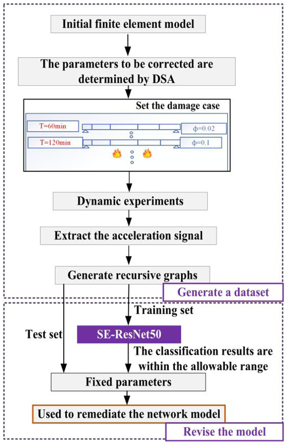
In response to the aforementioned limitations, a probabilistic damage risk assessment method that integrates improved deep residual network with FEM updating is proposed. First, the dynamic response data is transformed into RP format through phase space reconstruction, and the physical parameters of the initial FEM are updated using an enhanced residual network. Next, a dataset is constructed based on the static information from the updated FEM to achieve prediction of static reduction coefficients. Subsequently, considering the need for multi-source information in the damage level evolution throughout the entire process, the multi-granularity spatial-temporal attention learning (MG-STAL) evaluation branch is introduced, along with the comprehensive index, multi-variable feature index (MVFI). Several probabilistic models, including the normal, Gamma, Weibull, and Beta distributions, are used to fit the measured data and determine the probability density functions for damage levels II_a, II_b, and III. Finally, by integrating the prior-based minimum expected loss (MEL) criterion with posterior probabilities, a comprehensive evaluation of the damage assessment results is achieved. This method not only significantly improves the accuracy of damage identification but also provides a novel solution for damage assessment in practical engineering applications.

Static testing and dynamic modal testing of corroded RC beams after fire exposure

Thirteen RC beams, each measuring 3 m in length, 0.15 m in width, and 0.30 m in depth, were designed. The detailed design of the components is shown in Figure 1. The following sections will provide a detailed description of the material properties, specimens, and experimental setup.

Figure 1.

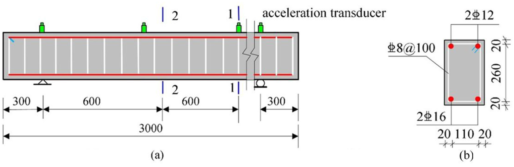
Design of corroded concrete beam: (a) beam section size and (b) reinforcement detailing of beam section.

Material properties

Concrete

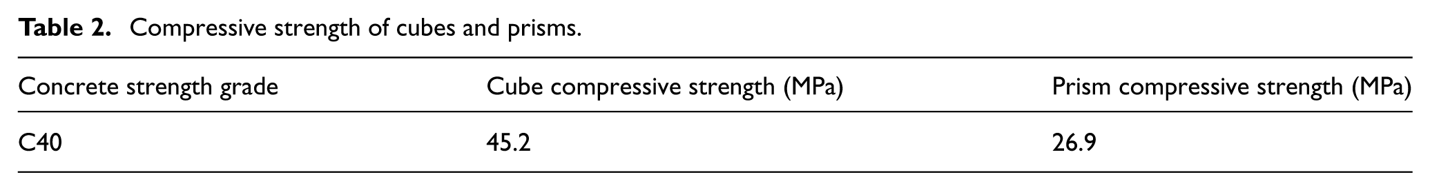
The beams were cast using C40 grade concrete. Table 2 presents the 28-day characteristic compressive strength of the concrete for cubic and prismatic specimens.

Table 2.

Compressive strength of cubes and prisms.

Concrete strength grade	Cube compressive strength (MPa)	Prism compressive strength (MPa)
C40	45.2	26.9

Steel

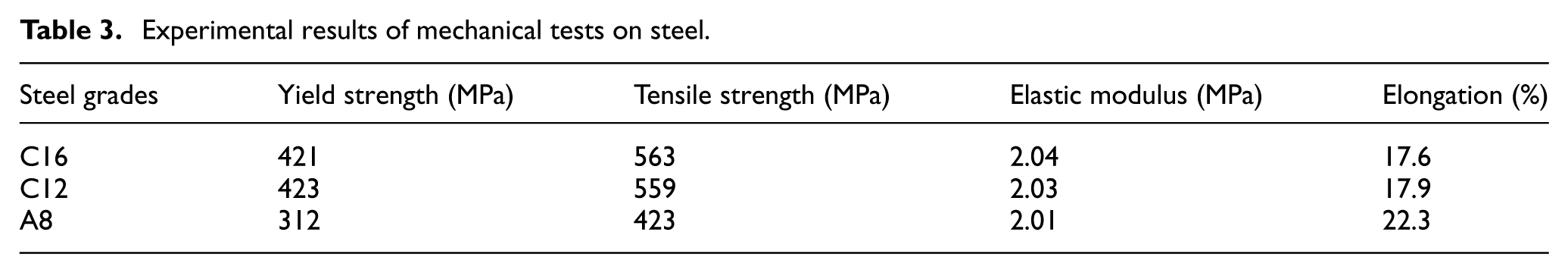
The tensile steel of the simply supported beam is designed using HRB400 steel bars with a diameter of 16 mm. The erection steel consists of HRB400 steel bars with a diameter of 12 mm, while the stirrups are made of HPB300 steel bars with a diameter of 8 mm, spaced at 100 mm intervals. The mechanical properties of the different steel grades are provided in Table 3, and the specific steel detailing is shown in Figure 2.

Table 3.

Experimental results of mechanical tests on steel.

Steel grades	Yield strength (MPa)	Tensile strength (MPa)	Elastic modulus (MPa)	Elongation (%)
C16	421	563	2.04	17.6
C12	423	559	2.03	17.9
A8	312	423	2.01	22.3

Figure 2.

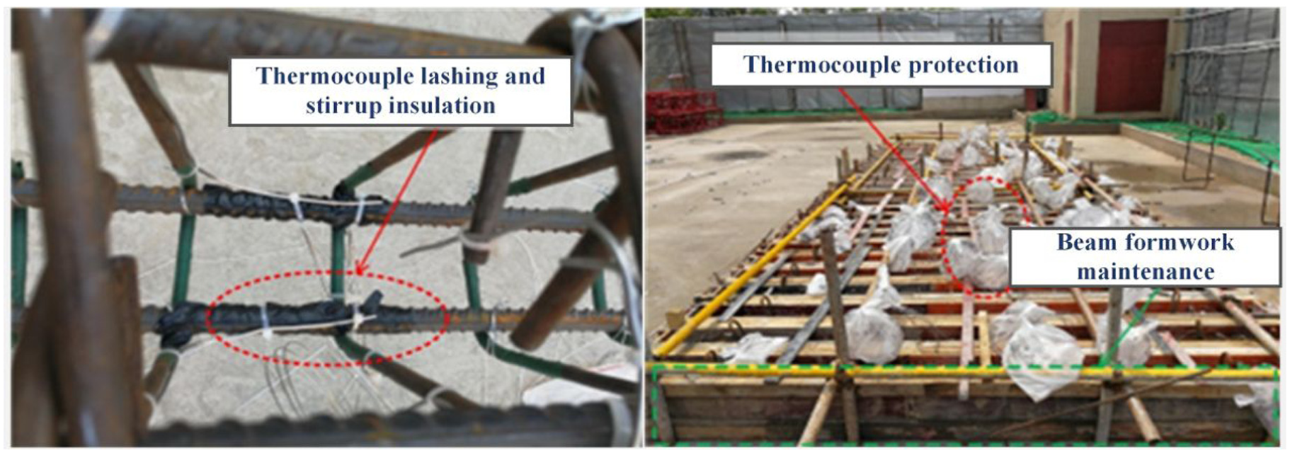
Setup for steel binding.

Corrosion testing setup

To ensure the reliability of the corrosion test, the method proposed in ASTM Standard G1-03²⁷ was followed. The steel bars were first cleaned with hydrochloric acid solution, followed by cleaning using a small hammer to remove any residual corrosion products adhered to the steel surface. Finally, the weight loss was measured to determine the total mass loss. Since this study focuses on the static reduction factor of corroded concrete beams and post-fire damage assessment, the spatial variability of corrosion²⁸ is not taken into account. Instead, the damage scenarios are defined solely by the average corrosion ratio. The formula for calculating the mass corrosion rate is as follows:

η_{s =} \frac{m_{0} - m}{m_{0}}

(1)

where m₀ is the mass of the steel before corrosion, and m is the mass after corrosion.

The corrosion test design is shown in Figure 3(a). The measured actual corrosion rate, determined using the above method, and the theoretical corrosion rate are shown in Figure 3(b). The results indicate that the deviation between the measured corrosion rate of the steel bars and the target corrosion rate remains within a small range, satisfying the accuracy requirements of the experiment.

Figure 3.

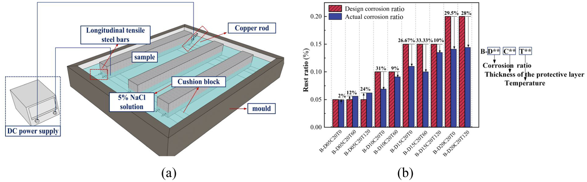
Design of corroded specimens: (a) corrosion test setup and (b) verification results of corrosion rate.

Fire and dynamic testing setup

Considering that the boundary conditions of fire may lead to different structural responses of the corroded concrete structure, the test was conducted by controlling the furnace temperature according to the ISO 834 heating curve. Temperature data were collected using a 34980A Hewlett-Packard Agilent device, with temperature monitoring set at 60-s intervals. Furthermore, the combustion control system automatically shuts off the burner to end the heating phase once the predefined fire temperature threshold is reached.

This study utilizes an excitation method to collect multi-domain dynamic information of fire-damaged corroded concrete beams. During the experiment, a DFC-2 medium-sized impact hammer was used as the excitation source, and impacts were accurately applied at specified loading points on both sides of the beam span. At the signal receiving end, a DHDAS dynamic signal acquisition system was employed to provide data support for subsequent model updates, static reduction identification, and probability distribution assessment based on multi-domain dynamic information. The detailed dynamic testing setup is shown in Figure 4.

Figure 4.

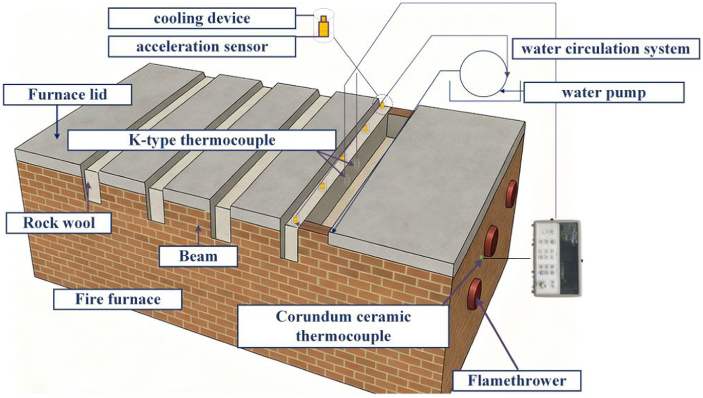
Experimental setup for fire and vibration tests.

Static testing setup

The static load test was conducted using an electro-hydraulic servo universal testing machine with a maximum load capacity of 500 kN. The test layout is shown in Figure 5. The loading method involves staged loading using jacks, with the load transferred through a distribution beam. The incremental load for each stage is 5% of the ultimate load (calculated to be 6 kN). To ensure the controllability of the loading process, the loading method switches from load control to displacement control when the steel reaches the yield stage. The loading increment is set to 3 mm at the mid-span deflection, continuing until the specimen fails. To verify the functionality of the equipment and the stability of the testing channel, three preloading tests were first conducted on the test beam. The preload was set at 30% of the theoretical cracking load threshold. Detailed explanations of the above test and structural response results can be found in reference.²⁹

Figure 5.

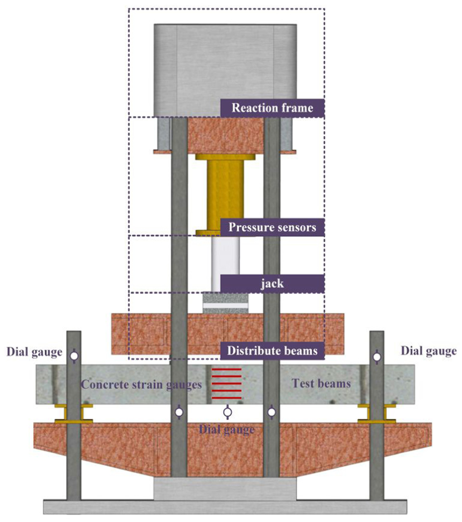
Static loading test.

Finite element simulation of fire-damaged corroded concrete beams

This study employs ABAQUS 2021 to perform numerical simulations and analyze the structural response of corroded concrete beams after fire damage.

Selection of element

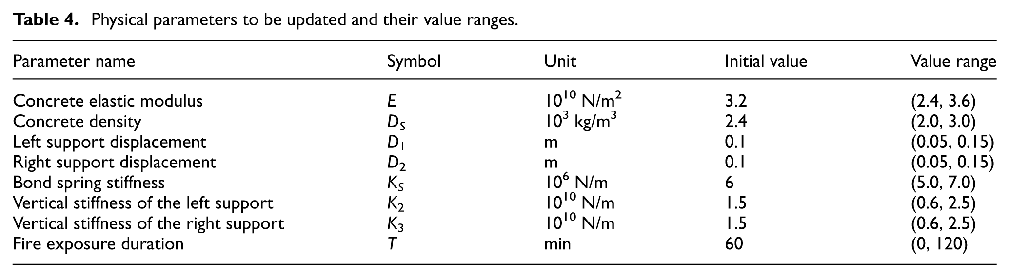
In the element selection, concrete and filler blocks are modeled using three-dimensional solid elements (C3D8R), while the steel is modeled using linear truss elements (T3D2). To allocate resources efficiently and improve the update speed, priority should be given to physical parameters that are sensitive to structural changes and can accurately reflect the structural conditions,³⁰ as detailed in Table 4.

Table 4.

Physical parameters to be updated and their value ranges.

Parameter name	Symbol	Unit	Initial value	Value range
Concrete elastic modulus	E	10¹⁰ N/m²	3.2	(2.4, 3.6)
Concrete density	D _S	10³ kg/m³	2.4	(2.0, 3.0)
Left support displacement	D ₁	m	0.1	(0.05, 0.15)
Right support displacement	D ₂	m	0.1	(0.05, 0.15)
Bond spring stiffness	K _S	10⁶ N/m	6	(5.0, 7.0)
Vertical stiffness of the left support	K ₂	10¹⁰ N/m	1.5	(0.6, 2.5)
Vertical stiffness of the right support	K ₃	10¹⁰ N/m	1.5	(0.6, 2.5)
Fire exposure duration	T	min	60	(0, 120)

Mesh partitioning and boundary conditions

The quality of mesh partitioning significantly impacts the accuracy of numerical model results. To obtain convergent characteristic solutions, the mesh size is set to 10 mm× 10 mm× 10 mm, resulting in a total of 152,126 elements. During the modeling process, accurately simulating the actual boundary conditions is challenging, as the translational and rotational boundary stiffnesses are usually limited.³¹ To simulate the approximate simply supported elastic boundary conditions for the corroded concrete beam, linear spring elements are introduced at the boundary nodes, the translational and rotational directions of which are defined.³⁰ These spring elements are also used to simulate the bond stress between the steel and concrete.^32,33 Specifically, the SPRING1 element is used to simulate foundation constraints, with the vertical stiffness at the left and right sides defined as K2 and K3. The stiffness values are determined based on engineering practices. The SPRING2 element simulates the bond stress between corroded steel and concrete. Considering the influence of corrosion on the bond performance, a stiffness reduction method is employed to characterize bond deterioration.³⁴ The reduction of the SPRING2 horizontal stiffness (K_S) is determined based on a degradation model.³⁵ In practical engineering, steel sliding mainly occurs along the x-axis. The stiffness in the other two directions is set to its maximum, assuming no sliding in those directions. The mesh partitioning and boundary conditions for each component are shown in Figure 6.

Figure 6.

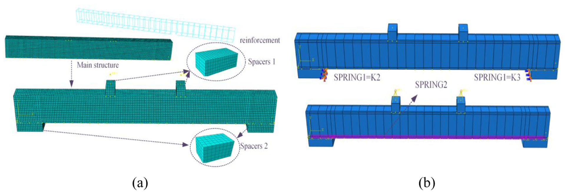
Establishment of the initial model: (a) mesh generation of the main structural beam, cushion blocks, and steel; (b) boundary constraints of the FEM. FEM: finite element model.

Temperature field simulation and dynamic data acquisition

In the temperature field setting, the same heating curve as in the actual working conditions is applied. The influence of temperature-dependent material properties, such as specific heat, thermal expansion coefficient, and thermal conductivity, is also considered. The thermal conductivity is determined by introducing the Stefan–Boltzmann constant. By setting different fire exposure durations, the damage degree of the concrete beam is observed. The FEM temperature field results are shown in Figure 7. As the fire exposure time increases, the internal temperature field of the concrete structure continues to extend inward, with the high-temperature zone slightly deepening. The internal temperature gradient decreases, indicating that heat is gradually conducted to deeper layers. It is noteworthy that the difference in surface temperature between the concrete structure exposed to fire for 90 and 120 min is minimal. This is mainly due to the concrete surface and the flame having reached thermal equilibrium, with the surface temperature stabilizing and further increases in temperature being less noticeable.

Figure 7.

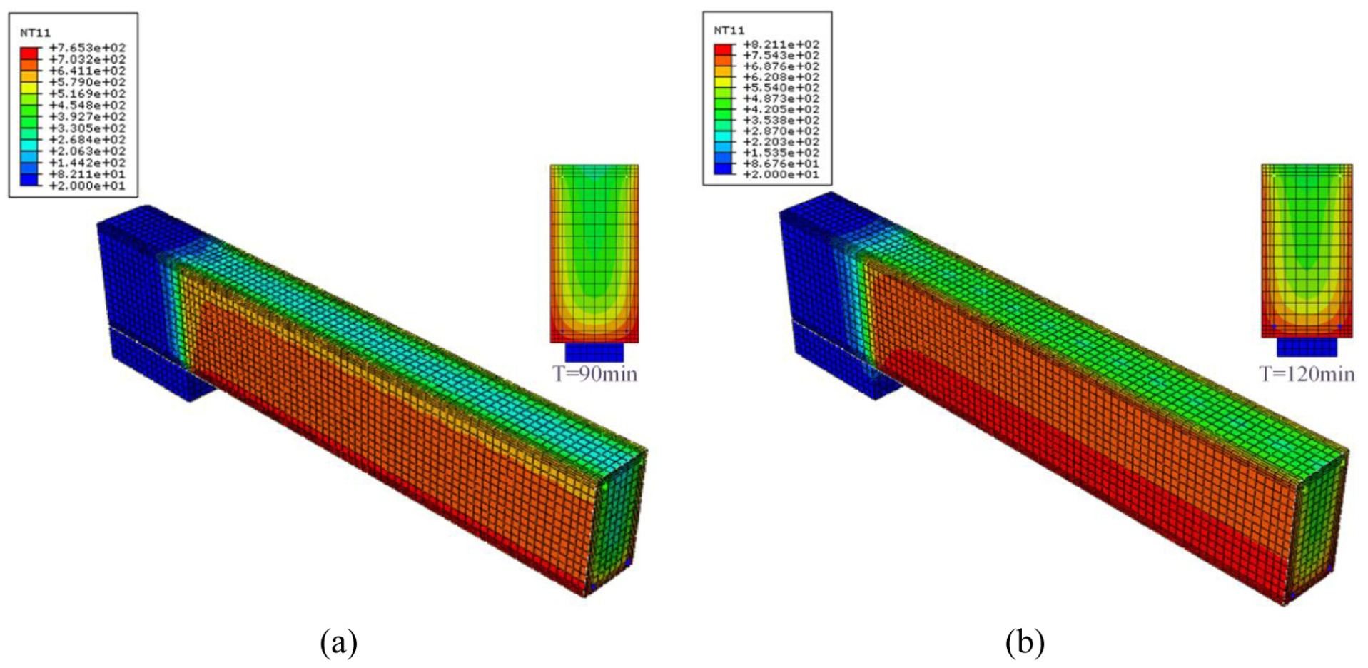
Temperature field simulation under different fire durations: (a) 90 min and (b) 120 min.

To verify the effectiveness of the temperature field model, temperature measurement points are selected at the locations of the steel stirrups and the geometric center of the component for comparative analysis. Since the stirrup position is closer to the high-temperature environment during the fire, the temperature gradient at measurement point 3 is large. The geometric center point can reflect the internal heat transfer characteristics of the component. By comparing the experimental testing (ET) and FEM temperature data at these two points, the rationality of the model’s temperature field distribution is validated. The results show that the ET temperature data measured by the 34980A Hewlett-Packard Agilent instrument closely align with the FEM calculation results. The FEM temperature information is shown in Figure 8, and the detailed study is shown in the reference.³⁶

Figure 8.

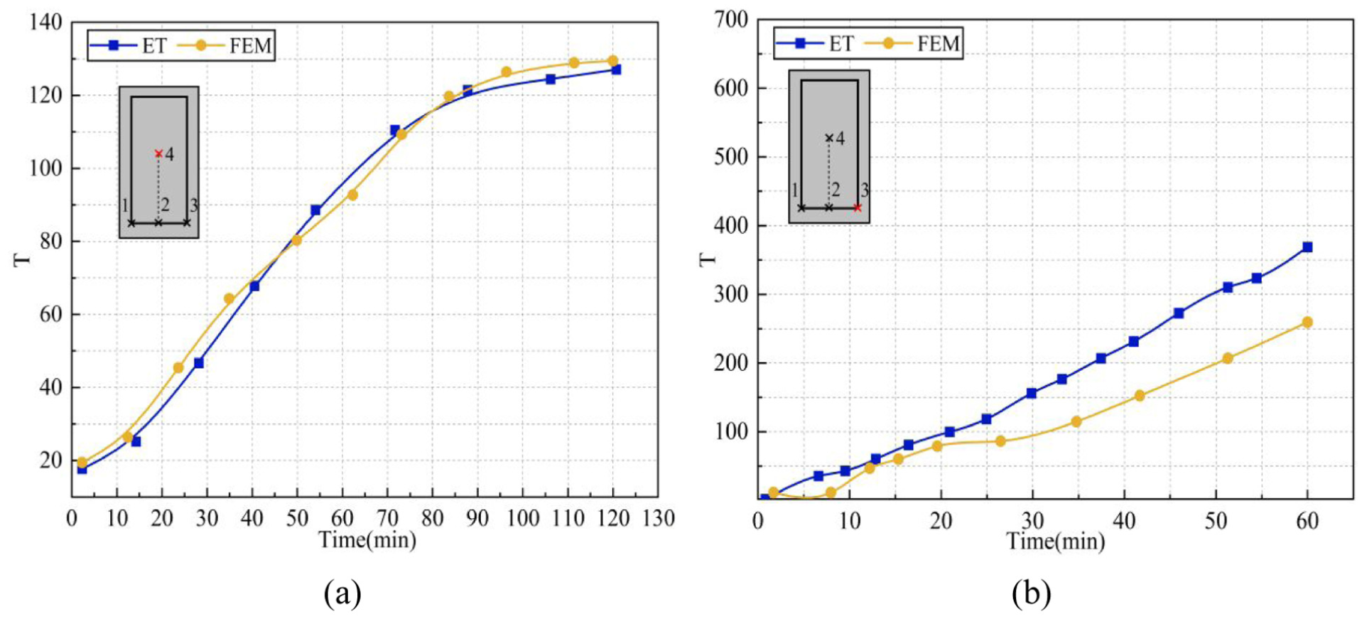
Validation of FEM temperature predictions against ET measurements at different positions: (a) ET and FEM temperature curves at the fourth selected point and (b) ET and FEM temperature curves at the third selected points. FEM: finite element model; ET: experimental testing.

For the component subjected to the applied temperature field, script programming is used to extract acceleration signal data at the quarter-span position from the data acquisition points. The quarter-span point effectively reflects the changes in the dynamic characteristics of the component under fire exposure, while avoiding local influences from the support constraint region and the mid-span extreme points. The experimental sampling frequency is set to 100 Hz with a sampling duration of 5 s, and the excitation direction is perpendicular to the top surface of the structure. To obtain the necessary parameters for constructing the RP, the autocorrelation function and false nearest neighbor algorithm are used to determine the time delay and embedding dimension of the acceleration signal, and phase space reconstruction is applied to form the RP data.

Correlation between experimental modal testing and FEM

The Modal Assurance Criterion (MAC) proposed in Equation (2) is used to determine the correlation between the model and experimental results.³⁷ This section compares the experimental dynamic response results with the FEM results. The dynamic response errors encompass errors in both natural frequencies and mode shapes. Since the errors in natural frequencies can be analyzed through the evaluation of mode shapes, this section focuses solely on the MAC analysis of mode shape errors. The MAC is defined as follows:

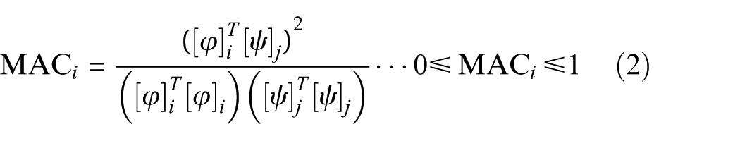
{MAC}_{i} = \frac{{({[φ]}_{i}^{T} {[ψ]}_{j})}^{2}}{({[φ]}_{i}^{T} {[φ]}_{i}) ({[ψ]}_{j}^{T} {[ψ]}_{j})} \dots 0 \leq \underset{i}{MAC} \leq 1

(2)

where [φ] is the modal vector of the ith mode in the experimental model, and [ψ] is the modal vector of the jth mode in the theoretical model. When MAC ≥ 0.8, it is considered that the correlation between the modal vectors is strong.

The third-order mode is extracted from the experimental dynamic data using frequency-domain methods and compared with the third-order mode from the FEM. The results in Figure 9(c) indicate slight interference in the second and third modes, suggesting that further adjustments to the physical parameters are required.

Figure 9.

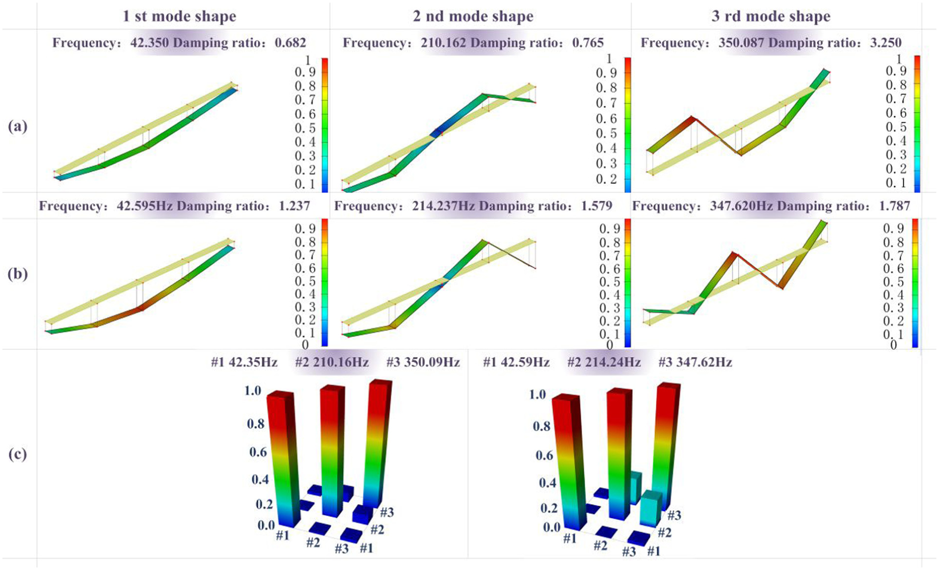
The first three vibration modes and natural frequencies of the specimens: (a) third-order mode shapes of specimen B-D15C20T60; (b) third-order mode shapes of specimen B-D15C30T60; (c) MAC correlation coefficients of the two specimens. MAC: Modal Assurance Criterion.

DSA sensitivity analysis

The efficacy of FEM updating is heavily predicated on the appropriate selection of updating parameters. While global sensitivity analysis method offers a comprehensive view of the parameter space, direct sensitivity analysis (DSA) is employed in this study. DSA is particularly advantageous for gradient-based optimization algorithms used in model updating, as it directly quantifies the local gradient of the structural response with respect to physical parameters, ensuring rapid convergence near the operational point.

The sensitivity analysis results, presented in Figure 10, identify the concrete density, elastic modulus, and fire exposure time as the most critical parameters affecting both static and dynamic responses. The underlying mechanisms for their high sensitivity are analyzed as follows:

Elastic modulus (E): This parameter is the dominant factor governing the stiffness matrix. Physically, the degradation of E due to high temperature directly leads to increased static deflection and reduced natural frequencies. Therefore, slight variations in E result in significant fluctuations in the objective function.

Fire exposure time (T): As a time-dependent variable, this parameter dictates the heat transfer and the extent of material degradation within the concrete cross-section. It acts as a hyper-parameter that controls the spatial distribution of material properties, thereby exhibiting high sensitivity regarding the global structural performance.

Density (D_S): Although mass loss during fire is relatively small compared to stiffness degradation, the density directly constructs the mass matrix. In dynamic assessments, even minor uncertainties in mass distribution can significantly alter the modal frequencies.

Figure 10.

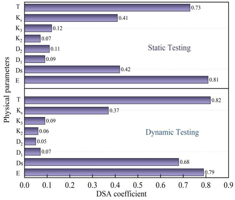
DSA sensitivity analysis for identifying parameters to be corrected. DSA: direct sensitivity analysis.

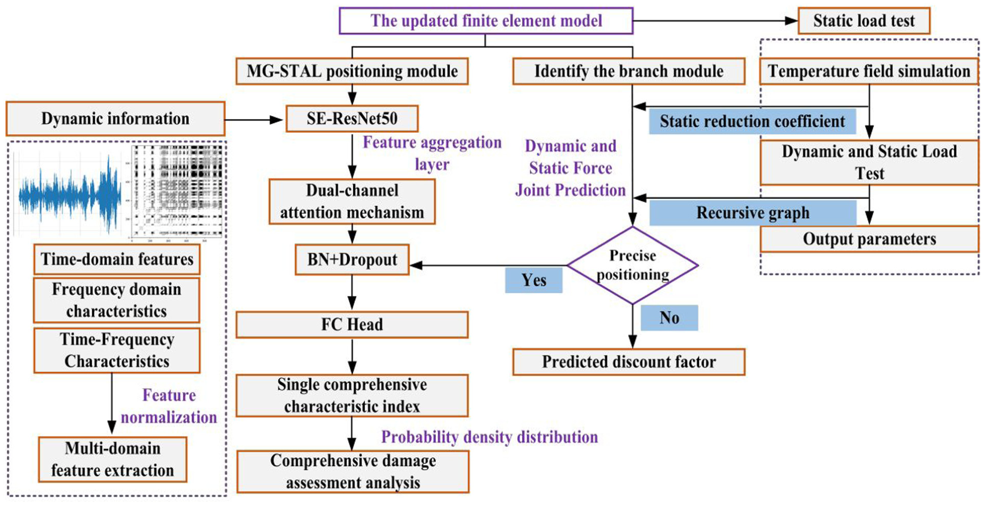
Parallel recognition and evaluation method based on the corrected model: SE-ResNet50 and MG-STAL

This study follows a parallel dual-branch strategy, jointly addressing two key aspects: static load reduction factor identification and full-process damage assessment. The first module is responsible for dynamic signal damage detection, where the time-domain signals are processed into RPs using the method of phase-space reconstruction. Due to clear limitations in experimental control conditions, a detection framework based on the corrected FEM is proposed. SE-ResNet50 performs pre-processing update on the FEM branch structure and further tracks significant changes in the static load reduction factor based on the corrected model. The update work of the SE-ResNet50 network is shown in Figure 11. This network takes RPs as input and outputs the physical parameters of model, enabling the update of critical FEM parameters. However, focusing only on the static load reduction factor is insufficient for a comprehensive damage assessment. Therefore, the MG-STAL module, which integrates multi-domain information, is used to evaluate the damage level. Once the system detects a performance reduction, it uses multi-domain information for further damage evaluation.

Figure 11.

Strategy for model update.

Damage identification and full-process assessment strategy

The dual-branch parallel recognition and evaluation method utilizes residual units and the MG-STAL module for deep feature extraction on the dynamic response of the updated FEM, comprehensively characterizing the structural dynamic behavior. This method integrates multi-domain features from both the structural time-domain and frequency-domain, generating a unified high-dimensional feature vector that preserves damage-sensitive information from different modes in a single metric. To improve the accuracy of recognition and evaluation, the framework incorporates a spatial-channel joint attention mechanism that adaptively enhances effective features from various types of dynamic information, enabling precise damage identification and evaluation evolution analysis. The detailed strategy is shown in Figure 12.

Figure 12.

Strategy for identification and comprehensive process evaluation.

Recognition branch structure: SE-ResNet50

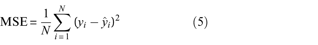
VGG16,³⁸ LeNet-5,³⁹ support vector machine (SVM),⁴⁰ and ResNet50⁴¹ are employed to process the same batch of RP data, aiming to explore the ability of the main network to extract dynamic information from RPs. The ability to extract nonlinear data is quantified using cosine similarity S (Equation (3)), classification accuracy A (Equation (4)), and root mean square (RMS) error (MSE) (Equation (5)), with the results shown in Table 5.

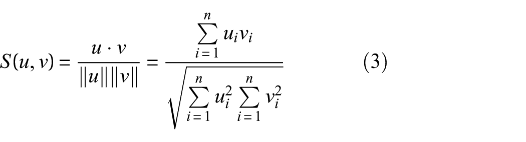
S (u, v) = \frac{u \cdot v}{‖ u ‖ ‖ v ‖} = \frac{\sum_{i = 1}^{n} u_{i} v_{i}}{\sqrt{\sum_{i = 1}^{n} u_{i}^{2} \sum_{i = 1}^{n} v_{i}^{2}}}

(3)

where u and v are the feature vectors to be compared.

A = \frac{{N_{t}}_{otal}}{{N_{c}}_{orrect}}

(4)

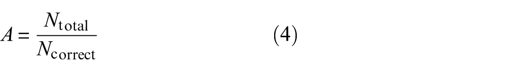
where N_correct is the number of correctly predicted samples and N_total is the total number of samples.

MSE = \frac{1}{N} \sum_{i = 1}^{N} (y_{i} - {\hat{y}}_{i})^{2}

(5)

where $y_{i}$ represents the true values, ${\hat{y}}_{i}$ represents the predicted values, and N is the total number of samples.

Table 5.

The effects of different models on the processing of nonlinear data.

Models	S	A	MSE
VGG16³⁸	0.88	0.86	0.89
CNN³⁹	0.84	0.81	0.87
SVM⁴⁰	0.78	0.74	0.75
ResNet50⁴¹	0.93	0.91	0.94

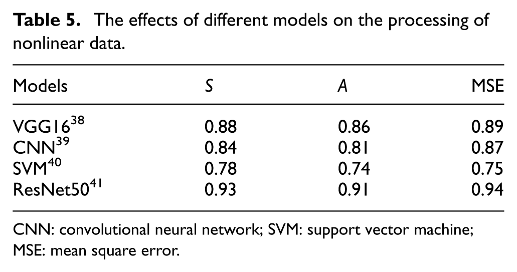
CNN: convolutional neural network; SVM: support vector machine; MSE: mean square error.

Based on the analysis of Table 5, it can be concluded that traditional learning methods such as SVM demonstrate limited performance in processing high-dimensional nonlinear image features. CNN and VGG16 networks lack stable information processing capability, particularly in terms of accuracy, error control, and robustness. In contrast, ResNet50 performs better due to the stable training advantages provided by its residual structure. Therefore, the residual structure is adopted as the main framework for processing nonlinear information. To investigate the differences in the focus of various models on the RP feature regions, Grad-CAM is used for visual analysis, as shown in Figure 13. The results indicate that the residual network can effectively focus on important areas of the RP but still overlooks the dynamic information in the edge regions. To address this limitation, an attention mechanism focusing on local edges is proposed.

Figure 13.

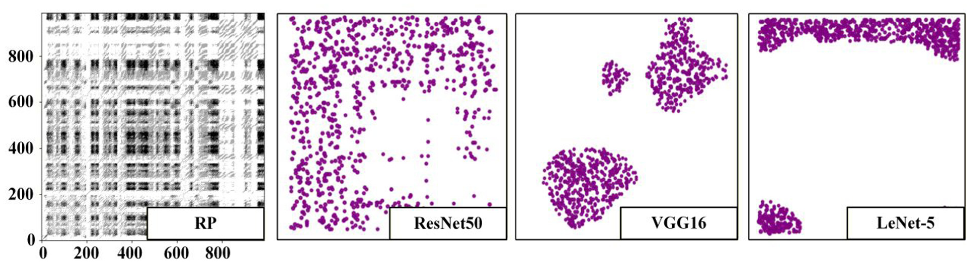
Differences in regions of interest for RP features across different models. RP: recurrence plot,

To enable the residual network to focus more on dynamic information, this study investigates current single attention mechanisms, including squeeze-and-excitation (SE) block, convolutional block attention module (CBAM), efficient channel attention (ECA), and bottleneck attention module (BAM). The main features and differences of these attention mechanisms are shown in Table 6. Among them, SE has a reasonable parameter size, computational load, and inference time. Although its parameter count is slightly higher than ECA, it is still lower than CBAM and BAM, making it suitable for meeting addressing the potential needs for one-stop local deployment.

Table 6.

The effects of different models on the processing of nonlinear data.

Attention	Parameters (×10³)	Floating point operations (×10⁶)	Inference time (ms)
SE	2.5	0.05	0.45
CBAM⁴²	3.2	0.07	0.50
ECA⁴³	0.8	0.03	0.42
BAM⁴⁴	3.0	0.06	0.48

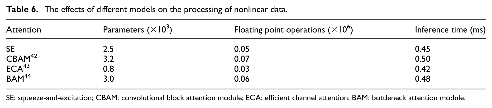
SE: squeeze-and-excitation; CBAM: convolutional block attention module; ECA: efficient channel attention; BAM: bottleneck attention module.

The SE-ResNet50 network architecture is shown in Figure 14. In stage 0, the initial feature extraction is performed using a 7 × 7 convolutional layer with 64 filters, followed by a 3 × 3 convolutional layer to further refine the features. Subsequently, the feedforward network processes the features nonlinearly using average pooling and the rectified linear unit activation function, enhancing the ability of the model to express the extracted features. Based on network improvements adapted from references,^45–47 a modified integration strategy is employed. Distinct from standard SE-ResNet implementations where SE blocks are embedded within every residual unit, this study introduces the SE attention mechanism between consecutive stages. Specifically, the SE module is placed after the final bottleneck block of stage i and before the initial block of stage i+1. This configuration allows the network to adaptively recalibrate the aggregated features of the current resolution level before passing them to the next hierarchical level. The SE block operates by accepting the output feature map from the previous stage, performing Global Average Pooling followed by a two-layer Fully Connected bottleneck to generate a channel-wise weight vector. These weights are then applied via element-wise multiplication to the feature map, effectively refining the input for the subsequent stage. Through the collaborative optimization of convolution, pooling, and attention modules in this multi-layer structure, the feature extraction and weight allocation processes are refined, significantly enhancing the representation of critical information and the extraction of edge features.

Figure 14.

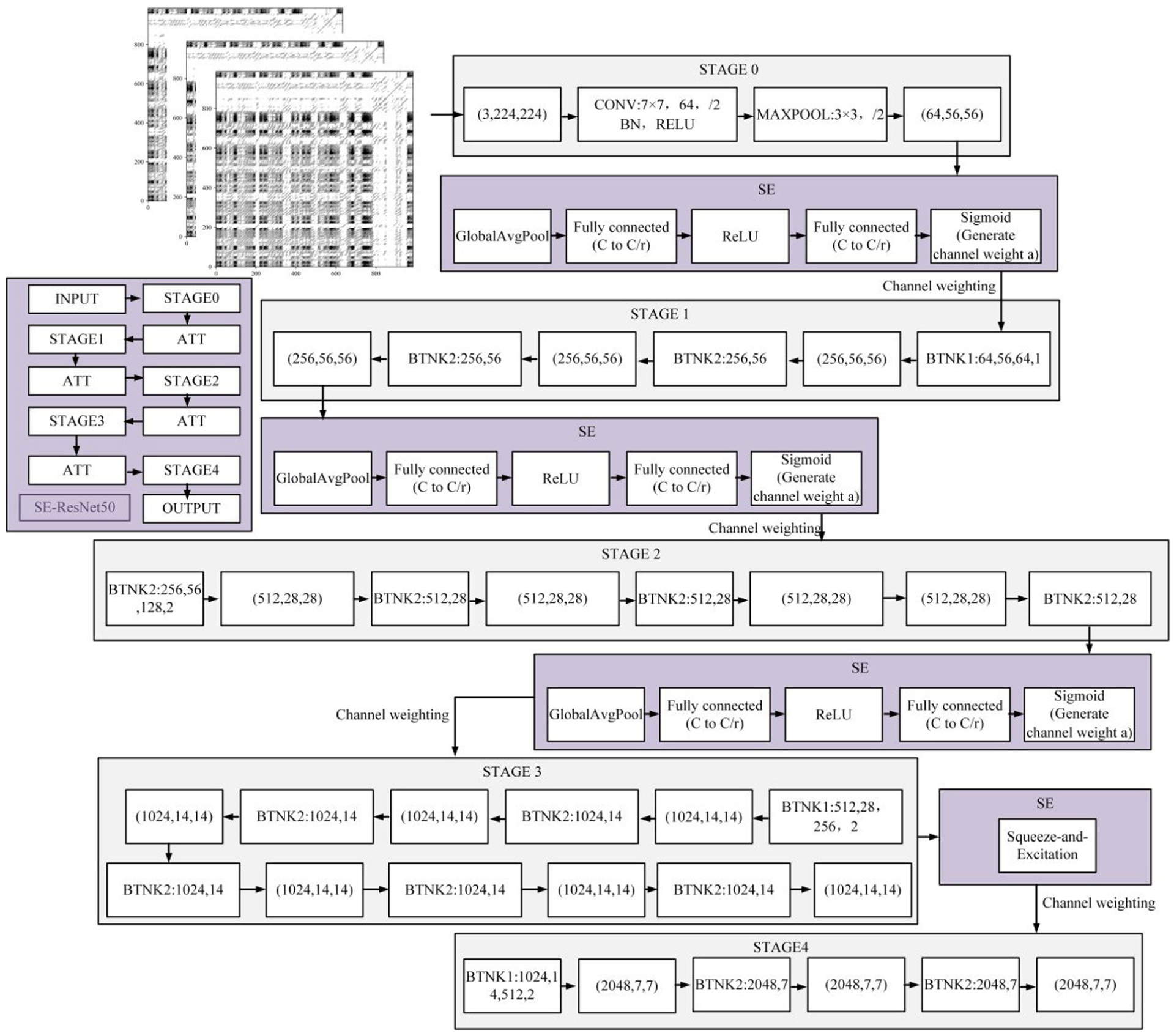
SE-ResNet50.

The RP dataset is input into both ResNet50 and SE-ResNet50 networks for training. The configuration is as follows: a batch size of 2, an initial learning rate of 0.001, which is kept constant during the process, and a total of 50 epochs. After the training is completed, the loss curve of the network is shown in Figure 15. The results indicate that SE-ResNet50 converges faster and achieves a lower convergence value in the later stages, demonstrating its superior feature extraction and classification capabilities compared to the baseline ResNet50 model.

Figure 15.

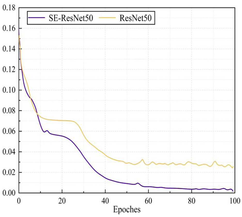
Training convergence of the network.

Multi-domain analysis and fusion-based damage assessment branch structure: MG-STAL

Multi-domain information extraction

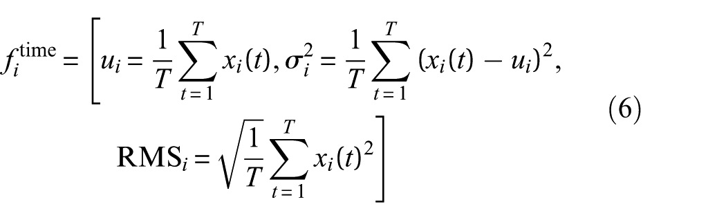
The extraction of dynamic information directly impacts the quality of recognition and evaluation. Therefore, multi-domain information, including time-domain, frequency-domain, and dynamic features, is extracted and consolidated into a unified feature matrix. In terms of time-domain feature extraction, representative indicators such as u, σ, and RMS are selected. For frequency-domain feature extraction, statistical features such as energy, spectral centroid frequency, and spectral bandwidth are selected. The response signal collected at sensor i be $x_{i} (t)$ , with a sampling length of T. The integrated time-domain feature vector can be represented as:

\begin{matrix} f_{i}^{time} = [u_{i} = \frac{1}{T} \sum_{t = 1}^{T} x_{i} (t), σ_{i}^{2} = \frac{1}{T} \sum_{t = 1}^{T} (x_{i} (t) - u_{i})^{2}, \\ {RMS}_{i} = \sqrt{\frac{1}{T}} \sum_{t = 1}^{T} x_{i} (t)^{2}] \end{matrix}

(6)

where $u_{i}$ represents the signal mean, $σ_{i}^{2}$ denotes the variance, and $RM S_{i}$ is the RMS, used to characterize the signal energy level. $x_{i} (t)$ represents the acceleration at the ith measurement point at time t.

The RMS extracted under different damage conditions are shown in Figure 16. It can be observed that the RMS at the support positions is relatively low, indicating a minimal impact on the overall dynamic information. In contrast, the influence at the mid-span and loading positions is higher, indirectly suggesting that the contribution of different measurement points to the damage differs.

Figure 16.

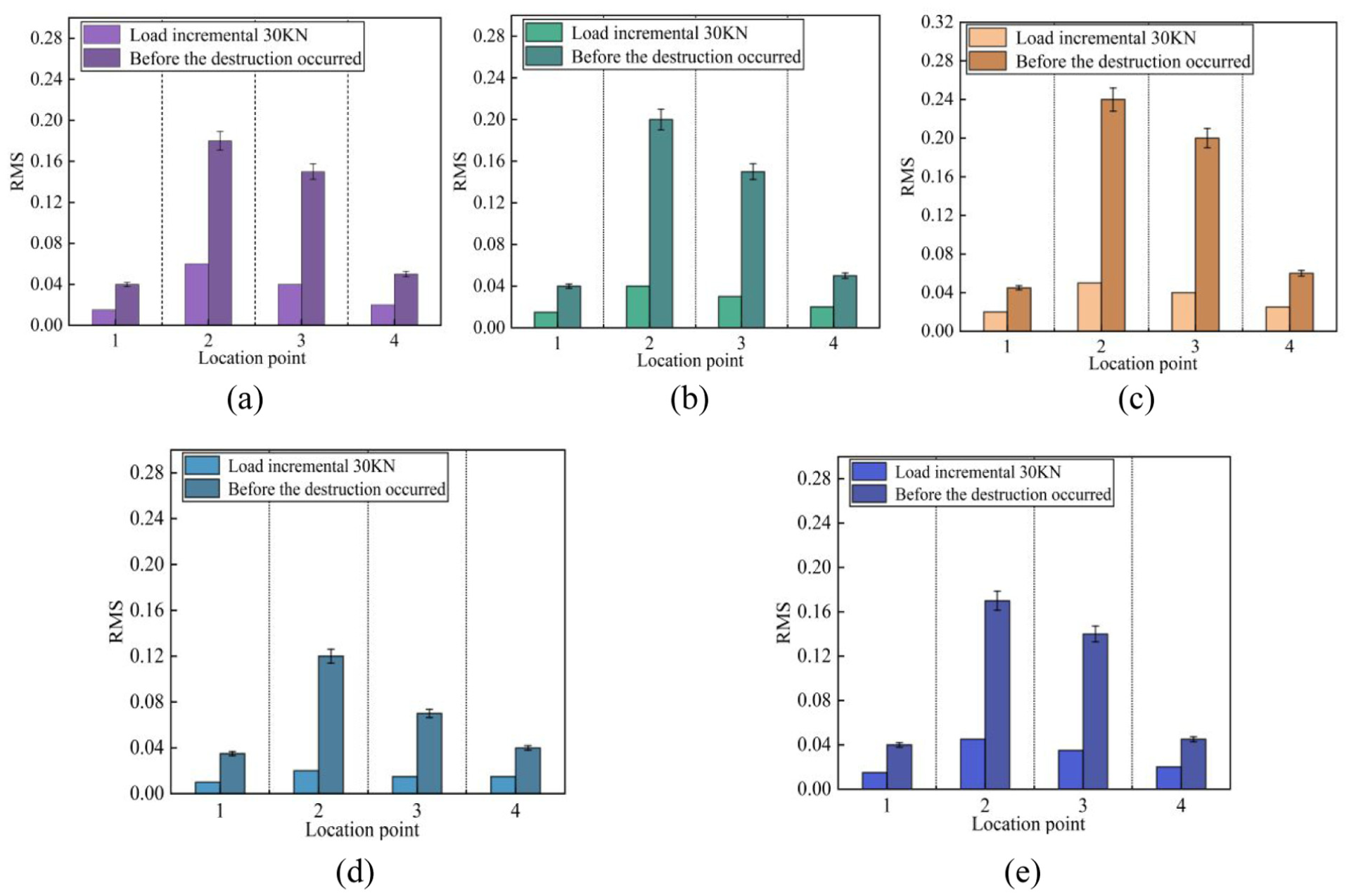
RMS under different damage conditions: (a) normal concrete beam; (b) corrosion rate 10%, fire exposure 60 min; (c) corrosion rate 10%, fire exposure 120 min; (d) corrosion rate 5%, fire exposure 60 min; and (e) corrosion rate 15%, fire exposure 60 min. RMS: root mean square.

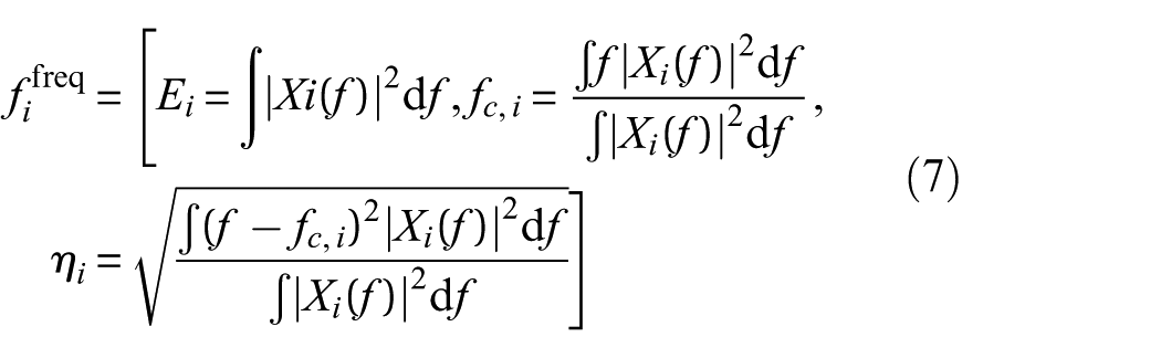
Frequency-domain features effectively reflect the time-domain variation patterns of the signal under different damage conditions, and their calculation is shown in Equation (7).

\begin{matrix} f_{i}^{freq} = [E_{i} = \int {| Xi (f) |}^{2} d f, f_{c, i} = \frac{\int f {| X_{i} (f) |}^{2} d f}{\int {| X_{i} (f) |}^{2} d f}, \\ η_{i} = \sqrt{\frac{\int {(f - f_{c, i})}^{2} {| X_{i} (f) |}^{2} d f}{\int {| X_{i} (f) |}^{2} d f}}] \end{matrix}

(7)

where $E_{i}$ represents the total energy, $f_{c, i}$ denotes the spectral centroid frequency, $η_{i}$ is the spectral bandwidth, and $X_{i} (f)$ is the magnitude spectrum of the signal at the $i$ th measurement point in the frequency domain.

To quantify the importance of different sensor measurement points in damage assessment, the damage level probability contribution rate $α_{i}$ is introduced. This contribution rate is defined based on the sensitivity of features from each measurement point and is used for feature fusion in the MG-STAL module.

α_{i} = \frac{S (X_{i})}{\sum_{j = 1}^{M} S (X_{j})}

(8)

where S(⋅) is the sensitivity mapping function, which amplifies the difference between high-sensitivity and low-sensitivity measurement points; X_i represents the multi-domain feature vector of the $i$ th measurement point; and M is the total number of sensors.

MG-STAL module for feature fusion

The extracted multi-dimensional features are input into the MG-STAL module for fusion processing. In the feature aggregation layer, a dynamic weight distribution mechanism is introduced, which combines attention and cross-branch attention to adaptively weight and interact with the multi-domain features. The residual structure in the aggregation layer ensures the integrity and transfer efficiency of the feature information. Fusion and deep enhancement are achieved through the collaborative interaction of batch normalization (BN), Dropout, and fully connected layers, aggregating into a comprehensive feature index (MVFI). MVFI quantitatively evaluates the overall structural performance change by normalizing and weighted fusion of multi-domain features. The weighted coefficients consider three core factors: multi-domain dynamic information, static reduction, and the highest surface temperature. The weight distribution is determined using the analytic hierarchy process⁴⁸ and the “Post-fire Structural Identification Standard” (T/CECS 252-2019). The final output MVFI parameters serve as key indicators for subsequent probability density distribution and damage level evolution analysis, providing reliable and stable feature representation for structural classification under different damage levels. The detailed module construction is shown in Figure 17.

Figure 17.

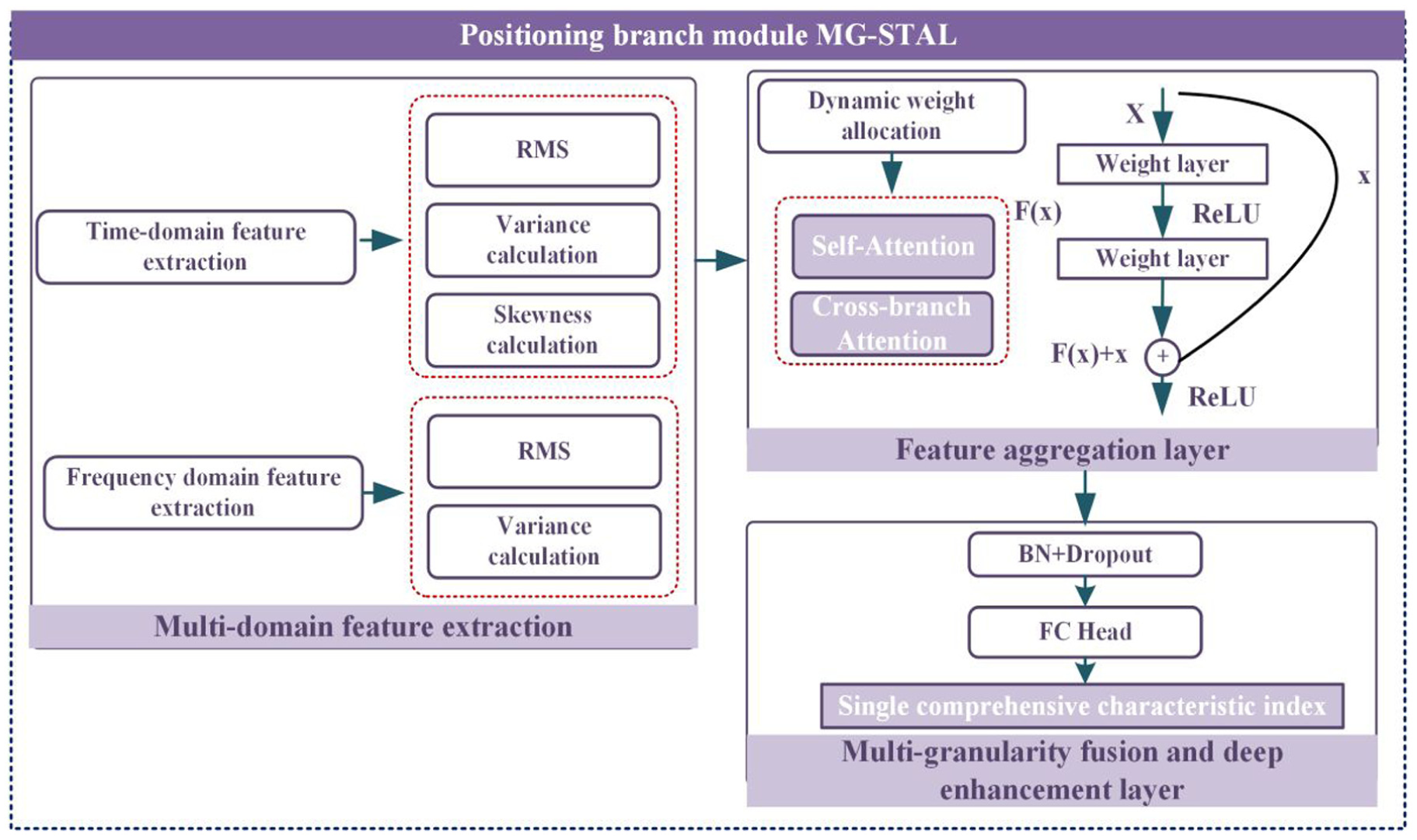
MG-STAL evaluation module.

The variation in the external load continuously affects the changes in the comprehensive index. This article investigates the variation rate of multi-domain dynamic information and static reduction factors at four measurement points as the load increases. The variation of the index for the comparison test beam without fire-induced corrosion is shown in Figure 18. As shown in the figure, with the increase in load, the MVFI accelerates during the yielding stage, and as the structure approaches its limit state, the growth rate gradually decreases. This phenomenon is primarily due to the fact that as the load increases, the beam structure approaches the yielding state, and the material begins to exhibit nonlinear deformation and plastic behavior, which results in a gradual reduction in structural stiffness. During the yielding stage, since the load-bearing capacity of structure has not yet reached its limit, accelerated deformation occurs, and the MVFI rapidly increases. However, once the structure reaches the limit state, the plastic deformation capacity of material is exhausted, and further load increases will not significantly affect the deformation and energy absorption capacity of the structure, resulting in a gradual slowdown in the growth rate of MVFI.

Figure 18.

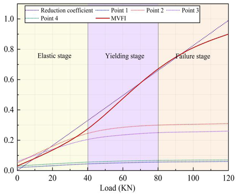
Variation of the MVFI comprehensive index of B-D00C20T00 under different loading conditions. MVFI: multi-variable feature index.

Corroded beams under different conditions exhibit distinct structural responses, which consequently influence the MVFI, as shown in Figure 19. Among them, the corrosion rate significantly impacts on MVFI, primarily because steel corrosion leads to degradation of the interface bond, reducing strain coordination between the concrete and steel. In terms of development rate, corrosion causes cracks to initiate earlier and expand faster, resulting in significant energy fluctuations in the dynamic and static indicators. Under the influence of fire, the overall stiffness of the concrete is reduced, material brittleness increases, and microcracks propagate after high-temperature exposure. As a result, the hysteretic characteristics of the structure weaken, leading to a reduction in the deformation capacity of the component. Under the same corrosion rate, high temperatures cause a slight increase in MVFI.

Figure 19.

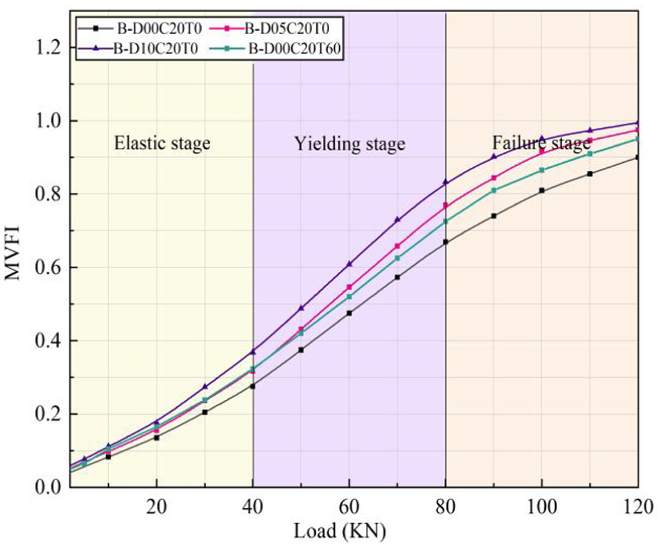
Effects of different conditions on the MVFI comprehensive index. MVFI: multi-variable feature index.

Probabilistic field-based damage assessment

In this study, owing to the lack of sufficiently representative field statistics for post-fire corroded RC beams, the prior probabilities of different damage levels were assumed as equal non-informative priors. Consequently, the posterior classification results are mainly governed by the fitted likelihood functions of the MVFI under different damage states. In future practical applications, these priors may be updated using field inspection records, long-term monitoring data, or expert knowledge to support project-specific probabilistic assessment. Meanwhile, uncertainty in the applied load may also affect the damage assessment results under fire conditions. Therefore, the MVFI proposed earlier was adopted as the reference index for probabilistic damage assessment. Since the uncertainty associated with external loads is generally much greater than that associated with structural geometry and has a more pronounced effect on structural response,⁴⁹ only the effect of external load uncertainty is considered in the present study.

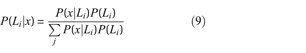
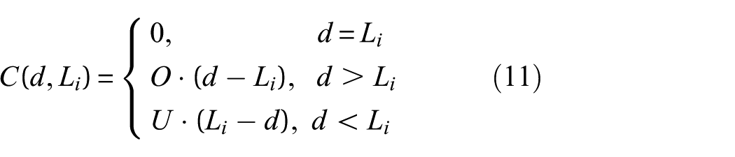
After verifying the reliability of the FEM data, five probability distribution functions (Normal, Gamma, Weibull, Beta, and Rayleigh) were employed to fit the probability data for three damage levels. The fitting accuracy of different distribution models for levels II_a, II_b, and III was quantitatively analyzed using the R² value, as shown in Table 7. The probability distribution fitting curves are shown in Figure 20(a), (b), and (c). The results indicate that the Gamma and Weibull distributions are the best probability distribution models for the corresponding damage levels. However, researchers often overlook the impact of load variations on structural damage during the assessment process.

Table 7.

Probability distribution function fitting.

Damage level	PDF	R ²
II_a	Normal⁵⁰	0.9775
	Gamma⁵¹	0.9940
	Weibull⁵²	0.9727
	Beta⁵³	0.9896
	Rayleigh⁵⁴	0.6615
II_b	Normal	0.9737
	Gamma	0.9844
	Weibull	0.9407
	Beta	0.9597
	Rayleigh	0.2465
III	Normal	0.9080
	Gamma	0.9076
	Weibull	0.9217
	Beta	0.9058

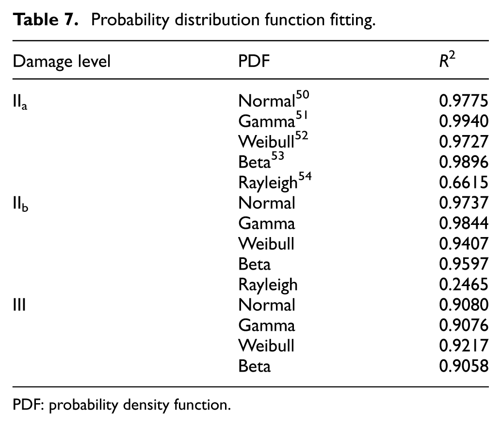
PDF: probability density function.

Figure 20.

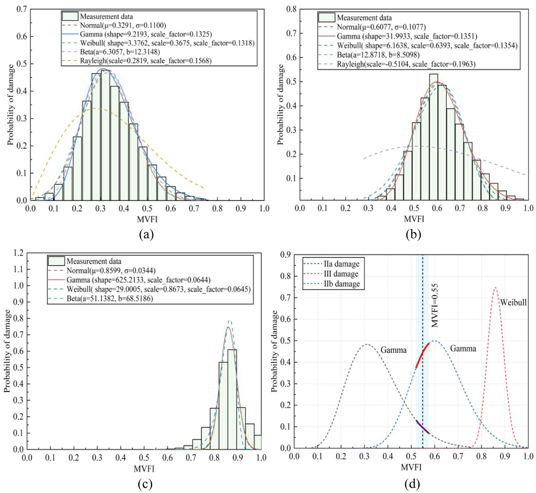
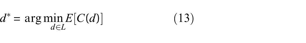
Probability density distribution of damage levels: (a) PDF of II_a damage level, (b) PDF of II_b damage level, (c) PDF of III damage level, and (d) PDFs of different damage levels. PDF: probability density function.

It is important to note that load variations can exacerbate structural damage. Figure 20(d) illustrates the occurrence probabilities of different damage levels under varying load conditions. As the damage deepens, the MVFI distribution shifts to the right and the fluctuation range decreases, indicating that this comprehensive index effectively distinguishes between different levels of damage. Additionally, Bayesian posterior probabilities are calculated based on the probability density functions for different levels, as shown in Equation (9).

P (L_{i} | x) = \frac{P (x | L_{i}) P (L_{i})}{\sum_{j} P (x | L_{i}) P (L_{i})}

(9)

where $P (L_{i} | x)$ represents the posterior probability of the ith damage level given the observed data x.

To automate the classification of damage levels, the category with the highest posterior probability is selected as the result, following the Maximum A Posteriori criterion, as shown in Equation (10).

d_{MAP} = \arg max_{i} P (L_{i} | x)

(10)

MEL criterion

Since the cost of misclassification in posterior probability is symmetric, it may underestimate safety risks. Therefore, the MEL criterion is introduced. Let the damage level set be L = {II_a, II_b, III}, the corresponding posterior probability vector P(L|x) ={P(II_a|x), P(II_b|x), P(III|x)}. When the determined level is d ∈ L and the true level is L_i the loss function is defined as:

C (d, L_{i}) = {\begin{matrix} 0, & d = L_{i} \\ O \cdot (d - L_{i}), & d > L_{i} \\ U \cdot (L_{i} - d), & d < L_{i} \end{matrix}

(11)

In the equation, U represents the loss coefficient caused by underestimating a level, and O represents the loss coefficient caused by overestimating a level. Considering that overestimation can usually be compensated for by engineering safety margins, while underestimation may lead to serious misjudgments in health monitoring. The corresponding expected loss $E [C (d)]$ is given in Equation (12).

E [C (d)] = \sum_{i} C (d, L_{i}) P (L_{i} | x)

(12)

where $C (d, L_{i})$ represents the loss function when decision d is made and the true level is L_i, and $P (L_{i} | x)$ is the posterior probability of the true level L_i, given the observed feature x.

Ultimately, the determination result is obtained by minimizing the expected loss, as shown in Equation (13).

d^{*} = \arg \underset{d \in L}{min E} [C (d)]

(13)

The sensitivity of the determination result to weight uncertainty is analyzed by studying the trend of E[C(d)] with relation to changes in U. The shaded region in Figure 21 represents the confidence interval for the weights mentioned above. From the figure, it can be observed that as U increases, the expected loss curves for each damage level gradually diverge. This phenomenon indicates that when the consequences of underestimating damage are assigned a higher weight, the optimal damage level determination shifts toward the more severe levels, II_b or III. This reflects the sensitivity of the MEL criterion in safety-oriented decision-making.

Figure 21.

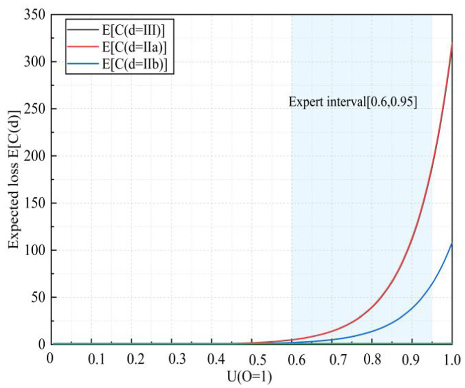
Expected loss of damage levels corresponding to different U values.

Network training and precision evaluation

The hardware configuration for the experiment is detailed in Table 8, which includes an Intel Xeon(R) E5-2699v3 processor running at 2.30 GHz, equipped with 2 × 128 GB of RAM and an NVIDIA GeForce RTX 3090 GPU with 24 GB of VRAM. In the software environment, PyCharm was utilized as the integrated development environment (IDE), while PyTorch was selected as the deep learning framework. During the training phase for model updating and recognition branches, a supervised learning approach was employed, optimizing model parameters by minimizing the discrepancy between predicted outputs and actual labels. To reduce training overhead and the required dataset size, a fine-tuning strategy was applied to the SE-ResNet50 network, ensuring adaptability to varying task-specific requirements. Moreover, an adaptive moment estimation (Adam) optimizer was employed to enhance convergence rates and overall model performance. Due to limitations in both data availability and computational resources, the training process was divided into eight sessions, each consisting of eight mini-batches, with a total of 100 training epochs. The initial learning rate was set to 0.001.

Table 8.

Main configuration of the model training workstation.

CPU	GPU	Environment setup and code execution	Deep learning framework
2 × 128 GB RAM Intel Xeon (R) E5 2699 v3 @ 2.30G Hz	1 × 24 GB Nvidia GeForce RTX 3090	PyCharm IDE	PyTorch

IDE: integrated development environment.

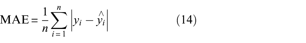
The mean absolute error (MAE) was chosen as the loss function to evaluate the performance of model updating and recognition, defined as shown in Equation (14).

MAE = \frac{1}{n} \sum_{i = 1}^{n} | y_{i} - \overset{\land}{y_{i}} |

(14)

where $y_{i}$ represents the true value of the $i$ th sample, and ${\hat{y}}_{i}$ represents the predicted value.

Experiment

Damage identification index

The reduction in bending capacity coefficient (γ_c) and bending stiffness reduction coefficient (γ_B) are used to characterize the degradation of bending capacity and stiffness of concrete beams under the combined effects of fire and corrosion.

γ_{c} = \frac{M_{c}}{M_{0}}

(15)

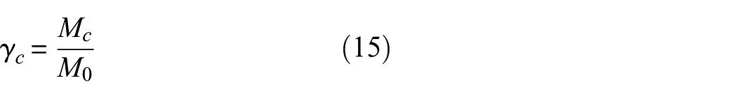
where M_c represents the bending capacity of the simply supported beam after corrosion and fire, while M₀ represents to the bending capacity of the uncorroded simply supported beam.

B = s \frac{M l_{0}}{f}

(16)

where B represents the stiffness of the tested beam, M represents the remaining bending capacity of the tested beam, s is the deflection coefficient, f is the mid-span deflection, and l₀ is the calculated span length.

γ_{B} = \frac{B_{c}}{B_{0}}

(17)

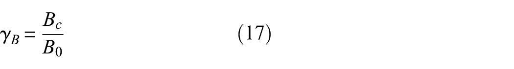
where B_c represents the bending stiffness of the simply supported beam after corrosion and fire exposure, while B₀ represents the bending stiffness of the simply supported beam that is neither corroded nor exposed to fire.

Dataset

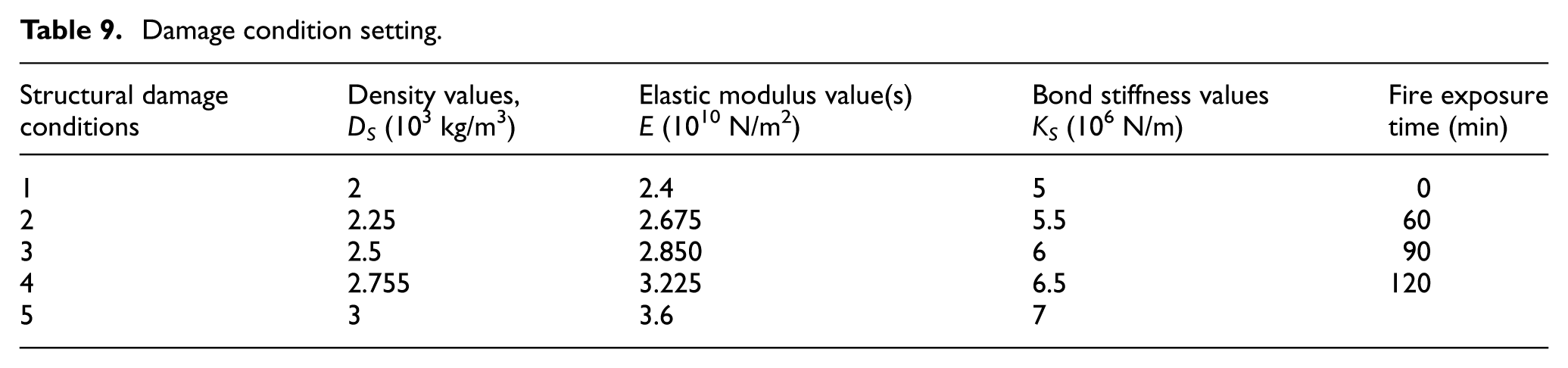
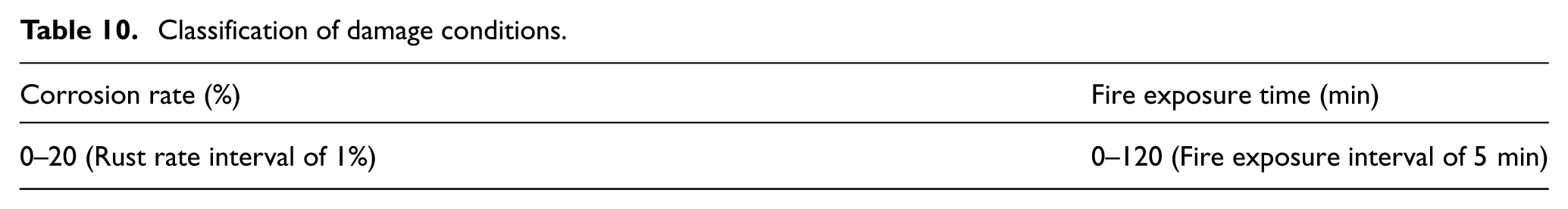
The quality of network training is directly influenced by the rationality of the dataset. To address this, a dataset was constructed by collecting dynamic information from key points of the model under different damage conditions. In the phase space reconstruction of the RP, two key parameters were set: the delay time (τ) was chosen as 2, and the embedding dimension (m) was set to 6. A total of 375 distinct damage conditions were designed, and data were collected from 25 measurement points across various operating conditions, resulting in 480 different damage states. The dataset was divided into training, validation, and test sets in a 7:2:1 ratio to assess the model’s generalization performance. To minimize the bias introduced by random splitting, five-fold cross-validation was employed in place of a single test set partition. The conditions for the FEM update and static identification tasks are detailed in Tables 9 and 10.

Table 9.

Damage condition setting.

Structural damage conditions	Density values, D_S (10³ kg/m³)	Elastic modulus value(s) E (10¹⁰ N/m²)	Bond stiffness values K_S (10⁶ N/m)	Fire exposure time (min)
1	2	2.4	5	0
2	2.25	2.675	5.5	60
3	2.5	2.850	6	90
4	2.755	3.225	6.5	120
5	3	3.6	7

Table 10.

Classification of damage conditions.

Corrosion rate (%)	Fire exposure time (min)
0–20 (Rust rate interval of 1%)	0–120 (Fire exposure interval of 5 min)

Ablation experiment

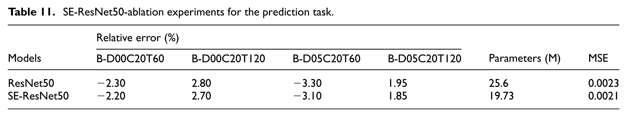
In “Recognition branch structure: SE-ResNet50,” a preliminary analysis of the loss and convergence effects during the training process of the attention mechanism was conducted. In this section, the results are further explained using three evaluation metrics: relative error, network parameters, and MSE. The prediction results for the static reduction factor are shown in Table 11. As shown in Table 11, the SE-ResNet50 variant achieves a reduction in the number of network parameters while maintaining or even improving the prediction accuracy. Meanwhile, the MSE is significantly reduced, indicating that the proposed model provides a more efficient and accurate feature representation. This improvement can be attributed to the channel attention mechanism introduced by the SE module, which adaptively recalibrates channel-wise feature responses and enables the network to focus on more informative features while suppressing less relevant ones. To test the generalization ability and update effect of the proposed SE-ResNet50 network, three representative damage conditions were selected from over 50 sets of independent test data. These data were not used during the training phase and were employed to independently assess the prediction accuracy and stability under real conditions, as shown in Figure 22. The results indicate that the parameter error of the SE-ResNet50 network is significantly reduced. The updated relative error is controlled within 5%, with the stiffness error of the L₂ spring dropping from 16.96 to 0.39%.

Table 11.

SE-ResNet50-ablation experiments for the prediction task.

Models	Relative error (%)				Parameters (M)	MSE
Models	B-D00C20T60	B-D00C20T120	B-D05C20T60	B-D05C20T120	Parameters (M)	MSE
ResNet50	−2.30	2.80	−3.30	1.95	25.6	0.0023
SE-ResNet50	−2.20	2.70	−3.10	1.85	19.73	0.0021

Figure 22.

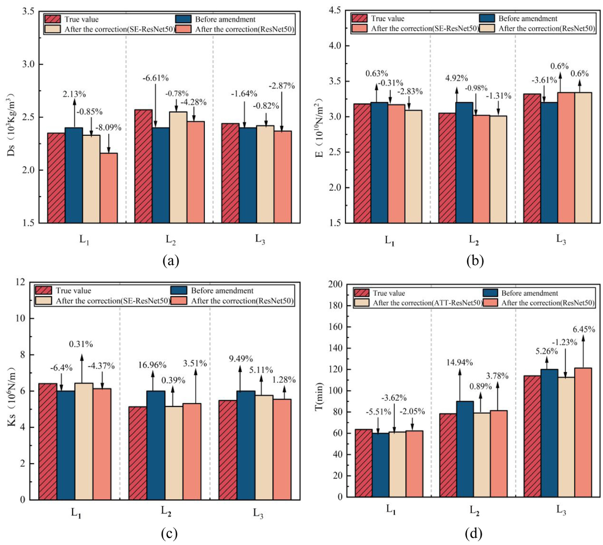
The results of the parameter update: (a) update results of D_S, (b) update results of E, (c) update results of K_S, and (d) update results of T.

Similar research was conducted on the MG-STAL module, and the results are shown in Table 12. After introducing the BN and Dropout modules, the model’s parameter count increased by approximately 3.4%, and the running time increased by 4.9%. However, the training process became more stable. Further introduction of the cross-channel attention mechanism increased the parameter count to 8.73 million and the running time rose to 36.8 s. Although the overall computational complexity slightly increased, both the feature expression capability and the overall performance of the model were significantly improved.

Table 12.

MG-STAL-comparative experiment.

Models				Parameters (M)	Times (s)
Self-attention	BN–Dropout	Cross-branch attention	Fully connected head	Parameters (M)	Times (s)
√				7.84	32.6
√	√			8.11	34.2
√	√	√		8.73	36.8
√	√	√	√	9.05	38.1

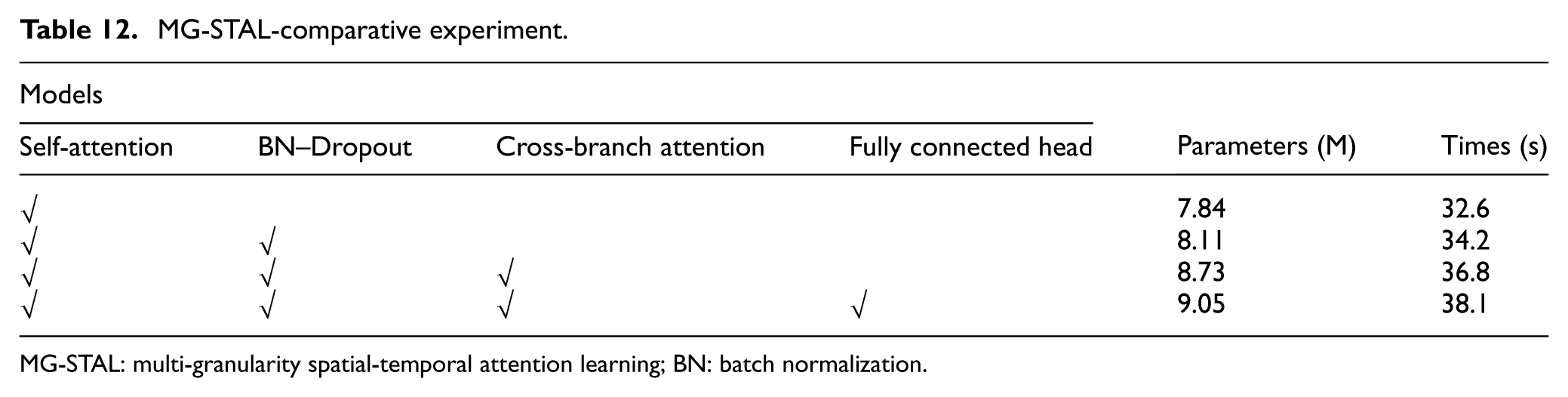
MG-STAL: multi-granularity spatial-temporal attention learning; BN: batch normalization.

Robustness against measurement noise and uncertainties

In practical engineering applications, the collected dynamic signals inevitably contain uncertainties arising from measurement noise, data sparsity, and model discrepancies. To specifically demonstrate the anti-interference capability of the proposed method against such uncertainties, a noise robustness analysis was conducted.

White Gaussian noise of varying intensities was added to the original acceleration signals to simulate different measurement conditions. The noise level is defined by the signal-to-noise ratio (SNR), with SNR values set to 30, 20, and 10 dB (a lower SNR indicates stronger noise interference). The noisy time-domain signals were then converted into RP and fed into the trained SE-ResNet50 model. The prediction errors for the static reduction factor under different noise levels are summarized in Table 13.

Table 13.

Maximum absolute relative error of static reduction factor under varying noise levels.

Test specimen	Models	Clean data (%)	SNR = 30 dB (%)	SNR = 20 dB (%)	SNR = 10 dB (%)
B-D00C20T60	ResNet50	2.30	2.75	3.55	4.85
B-D00C20T60	SE-ResNet50	2.20	2.52	3.12	4.15
B-D00C20T120	ResNet50	2.80	3.35	4.25	5.60
B-D00C20T120	SE-ResNet50	2.70	3.05	3.68	4.55
B-D05C20T60	ResNet50	3.30	3.85	4.72	6.25
B-D05C20T60	SE-ResNet50	3.10	3.42	3.95	4.85
B-D05C20T120	ResNet50	1.95	2.45	3.15	4.65
B-D05C20T120	SE-ResNet50	1.85	2.15	2.75	3.85

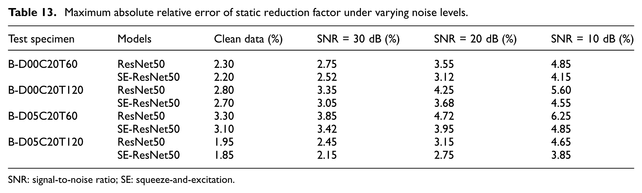
SNR: signal-to-noise ratio; SE: squeeze-and-excitation.

As shown in Table 13, while the prediction errors for all specimens inevitably increase with the introduction of noise, the proposed SE-ResNet50 model demonstrates exceptional robustness. For the baseline ResNet50 model, severe noise interference (SNR = 10 dB) causes the prediction error to degrade significantly, exceeding the 5% acceptable threshold in several cases (reaching up to 6.25% for specimen B-D05C20T60). In contrast, the maximum relative error of the SE-ResNet50 model remains well controlled within 5% across all tested specimens, peaking at only 4.85%. This robustness is primarily attributed to the RP transformation capturing topological structural features rather than exact amplitudes, combined with the SE attention mechanism that adaptively suppresses noise-dominant channels. Furthermore, the epistemic uncertainties arising from model discrepancies and data sparsity are effectively mitigated in the subsequent assessment stage by utilizing the probability distribution rather than deterministic hard labels.

Comparative experiment

Table 14 provides an initial evaluation of the network’s feature extraction capabilities. This study compares the performance of four mainstream recognition models: SVM, CNN, VGG16, and Transformer, by applying the same training strategy to each model. The results are presented in Table 14. It is evident that the ResNet50 model performs well across all metrics, with both relative error and MSE showing well results. In contrast, the VGG16 model, due to its larger number of parameters, is prone to overfitting, especially in small sample scenarios. Compared to ResNet50, the Transformer model demonstrates a further reduction in the average relative error by approximately 0.22% and a slight decrease in MSE by about 0.0001. This indicates superior generalization and feature representation capabilities. However, the Transformer model has a larger architecture and higher computational complexity, which makes it less efficient for deployment in engineering scenarios. Additionally, the recognition errors are relatively larger for scenarios where the corrosion rate exceeds 10% and the fire exposure time exceeds 60 min. This could be attributed to the complexity of the conditions, which interfere with the stability of dynamic information acquisition from the component, leading to discrepancies between the updated FEM and the actual component. As a result, the subsequent reduction factor identification tends to exhibit higher errors.

Table 14.

ResNet50-comparative experiment.

Models	Relative error (%)				Parameters (M)	MSE
Models	B-D00C20T60	B-D00C20T120	B-D05C20T60	B-D05C20T120	Parameters (M)	MSE
Transformer	−2.10	2.54	−3.00	1.83	33.58	0.0022
ResNet50	−2.30	2.80	−3.30	1.95	25.6	0.0023
VGG16	−4.85	5.32	−6.10	4.76	138.63	0.0048
CNN	−3.42	4.10	−4.25	3.27	9.86	0.0034
SVM	−5.00	5.80	−6.50	4.90	—	0.0055

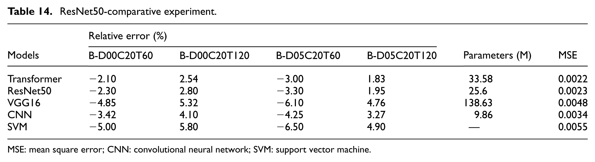
MSE: mean square error; CNN: convolutional neural network; SVM: support vector machine.

Damage level evolution

In this section, the dynamic and static response information from six experimental beams was integrated. Based on the proposed MEL criterion and probabilistic loss function, damage level determination and its evolution were analyzed. Table 15 presents the damage level evolution under static loads ranging from 30 to 90 kN for various damage conditions. The results show a high correlation between the loading conditions and the damage levels. As the fire exposure time increases, the distribution peak gradually shifts to the range of 0.45–0.61, and the expected loss E[C(d)] increases to 0.12–0.25. This indicates an evolution of the damage level from II_a to II_b, reflecting the cumulative effects of moderate damage. When fire damage becomes significant, the probability distribution shifts from Gamma to Weibull, with the mean further increasing to 0.72–0.86 and E[C(d)] growing rapidly to 0.38–0.63. At this stage, the structure enters a state of II_b–III, or even III level damage, with a significantly higher risk of underestimating damage. This trend suggests that as fire or corrosion damage worsens, the posterior probability gradually dominates, and the MEL criterion tends to favor more severe damage levels. Furthermore, the analysis of the damage level evolution throughout the entire process under load variations is presented in Table 16. It is evident that fire exposure and initial defects significantly reduce the damage threshold of the beam, causing severe degradation even at relatively low load levels.

Table 15.

Estimation of damage probability.

Damage conditions	Distribution type	μ	σ	MVFI	E[C(d)]	Damage level
B-D00C20T60	Gamma	0.329	0.110	0.33	0.05	II_a
B-D00C20T120	Gamma	0.45	0.09	0.45	0.12	II_a–II_b
B-D05C20T60	Gamma	0.608	0.108	0.61	0.25	II_b
B-D05C20T120	Gamma	0.72	0.07	0.72	0.38	II_b–III
B-D10C20T60	Weibull	0.80	0.05	0.80	0.52	III
B-D20C20T60	Weibull	0.86	0.034	0.86	0.63	III

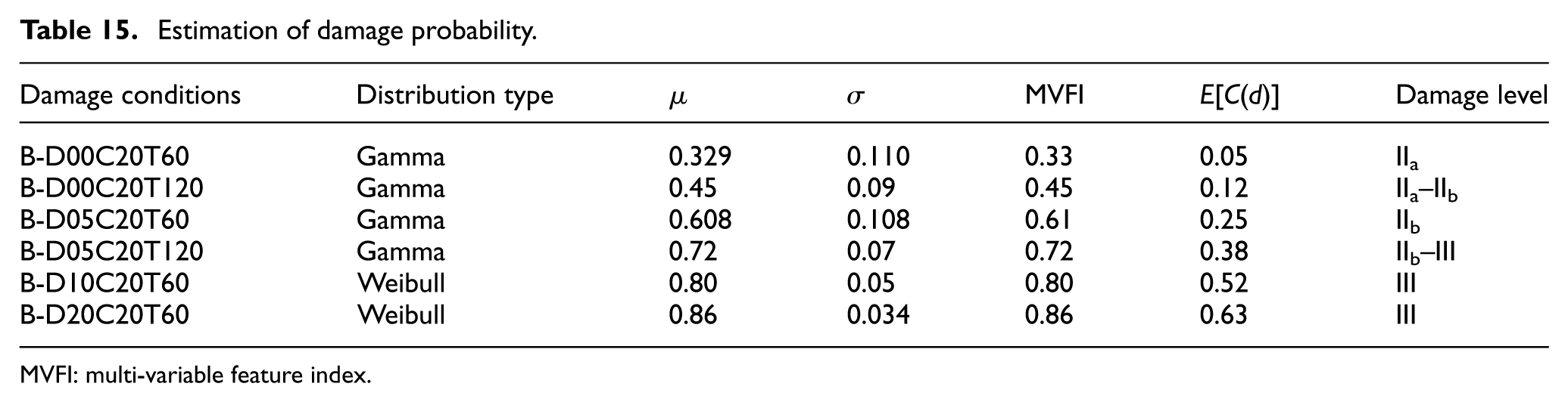
MVFI: multi-variable feature index.

Table 16.

Evolution of damage levels.

Damage conditions	Load (KN)			P _max
Damage conditions	II_a	II_b	III	P _max
B-D00C20T60	0–80.6	80.6–107.5	107.5–114.8	114.8
B-D00C20T120	0–64.2	64.2–84.6	84.6–92.5	92.5
B-D05C20T60	0–58.1	58.1–96.7	96.7–104.3	104.3
B-D05C20T120	0–47.5	47.5–63.1	63.1–69.8	69.8
B-D10C20T60	0–50.8	50.8–76.5	76.5–112.7	112.7
B-D20C20T60	0–43.9	43.9–68.2	68.2–98.2	98.2

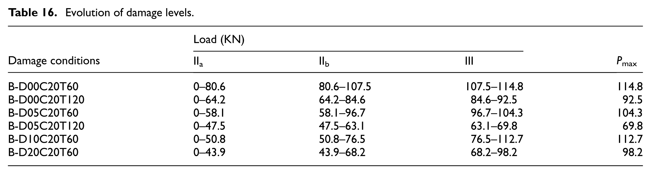
Conclusion

This study proposes a damage identification and probabilistic risk assessment framework for fire-damaged and corroded RC beams by integrating deep learning with multi-domain dynamic and static information. Compared with conventional FEM-ML-based damage identification approaches, the proposed framework places greater emphasis on nonlinear dynamic information representation, dynamic–static information fusion, and probabilistic damage assessment. The main conclusions are as follows:

The proposed neural network model effectively identifies the reduction factors for structural stiffness and bending capacity. The prediction results closely match the experimental data, confirming the feasibility of the method. Among different data types, using RP as the training dataset achieves higher recognition efficiency and accuracy.

In the FEM update and damage identification tasks, the SE-ResNet50 model performs well, with prediction errors kept within 5%. Compared to the baseline ResNet50 model, the recognition accuracy improves by 5–8%, demonstrating higher precision and reliability. When compared to existing mainstream backbone networks, the adopted residual network structure also shows a competitive advantage.

SE-ResNet50 shortens the training time and enhances computational efficiency. This method does not require multiple parameter outputs, providing a clear advantage in terms of computational efficiency. For model update tasks, it is recommended to use networks trained on RP datasets. In damage identification tasks, the choice of dataset, either RP or time-domain signals, can be adapted flexibly depending on the specific application scenario.

Based on the MG-STAL module and probability density analysis method, dynamic evolution of the damage levels in fire-damaged and corroded beams over their entire service life was evaluated. The results demonstrate strong consistency with prior probability analysis.

However, the current loading conditions considered are relatively simple. Future work could incorporate multidimensional loading scenarios, such as seismic and wind loads, and develop more comprehensive uncertainty models based on risk analysis. In addition, since actual corrosion is spatial and non-uniform in nature, future studies should investigate the spatial variability of corrosion (spatial corrosion). Integrating non-uniform corrosion models would allow for a more accurate characterization of local damage evolution and improve the effectiveness of assessment methods under realistic service conditions. Furthermore, when the residual identification method is applied to complex structures that differ significantly from the training data, its generalization performance may be limited. Therefore, improving the robustness and adaptability of the model under varying conditions remains an important direction for future research.

Footnotes

Appendix A

Appendix B

ORCID iD

Dalong Wang

Funding

The authors disclosed receipt of the following financial support for the research, authorship, and/or publication of this article: This study is sponsored by the National Natural Science Foundation of China (No. 52178487) and Natural Science Foundation of Shandong Province (No. ZR2021 ME228), to which the authors are very grateful.

Declaration of conflicting interests

The authors declared no potential conflicts of interest with respect to the research, authorship, and/or publication of this article.

References

Radzi

NAM

Hamid

Mutalib

, et al. A review of the structural fire performance testing methods for beam-to-column connections. Adv Civ Eng 2021: 1–18.

Lei

Guo

Dong

, et al. Life-cycle performance prediction and interpretation for coastal and marine prestressed concrete beams using active learning-enhanced Bayesian neural networks. Reliab Eng Syst Saf 2026; 265: 111557.

Wang

Guo

Jiang

, et al. Physics guided neural network framework for predicting shear strength of corroded reinforced concrete beams. Eng Fail Anal 2025; 181: 109970.

Guo

Dong

Bastidas-Arteaga

. Mixed Bayesian Network for reliability assessment of RC structures subjected to environmental actions. Struct Saf 2024; 106: 102392.

Mottershead

Friswell

. Model updating in structural dynamics: a survey. J Sound Vib 1993; 167: 347–375.

Shi

Lou

Yang

. Optimized machine learning methods for identifying the stiffness loss of CRTS-II slab track based on vehicle vibration signals. Adv Eng Inform 2024; 62: 102886.

Sha

Yue

Wang

. Ensemble 1D DenseNet damage identification method based on vibration acceleration. Struct Durab Health Monit 2023; 17: 369–381.

Cao

Liu

, et al. Vibration-based methods for local damage identification of breathing cracks in truss-like structures. J Sound Vib 2024; 592: 118646.

Razak

Choi

. The effect of corrosion on the natural frequency and modal damping of reinforced concrete beams. Eng Struct 2001; 23: 1126–1133.

10.

Chinka

SSB

Putti

Adavi

. Modal testing and evaluation of cracks on cantilever beam using mode shape curvatures and natural frequencies. Structures 2021; 32: 1386–1397.

11.

Hashim

Ibrahim

Razak

. Dynamic characteristics and model updating of damaged slab from ambient vibration measurements. Measurement 2013; 46: 1371–1378.

12.

Abdel Wahab

De Roeck

. Damage detection in bridges using modal curvatures: application to a real damage scenario. J Sound Vib 1999; 226: 217–235.

13.

Ndambi

J-M

Vantomme

Harri

. Damage assessment in reinforced concrete beams using eigenfrequencies and mode shape derivatives. Eng Struct 2002; 24: 501–515.

14.

Casas

Aparicio

. Structural damage identification from dynamic-test data. J Struct Eng 1994; 120: 2437–2450.

15.

Liu

Zhang

. Experimental study of structural damage identification based on modal parameters and decay ratio of acceleration signals. Front Archit Civ Eng China 2011; 5: 112–120. https://doi.org/10.1007/s11709-010-0069-3

16.

Brownjohn

JMW

Dumanoglu

Severn

. Ambient vibration survey of the Fatih Sultan Mehmet (second Bosporus) suspension bridge. Earthq Eng Struct Dyn 1992; 21: 907–924.

17.

Fang

S-E

Perera

De Roeck

. Damage identification of a reinforced concrete frame by finite element model updating using damage parameterization. J Sound Vib 2008; 313: 544–559.

18.

Ren

W-X

De Roeck

. Structural damage identification using modal data. II: test verification. J Struct Eng 2002; 128: 96–104.

19.

Shiradhonkar

Shrikhande

. Seismic damage detection in a building frame via finite element model updating. Comput Struct 2011; 89: 2425–2438.

20.

Steinwender

Nordmann

. Systematic correction of stiffness of a finite element model by means of measured eigenvalues and derivation of concrete identification factors of a dowel connection. Int J Press Vessel Pip 1987; 30: 87–107.

21.

Shahandashti

Ashuri

. Forecasting engineering news-record construction cost index using multivariate time series models. J Constr Eng Manag 2013; 139: 1237–1243.

22.

Ren

De Roeck

. Structural damage identification using modal data. I: simulation verification. J Struct Eng 2002; 128: 87–95.

23.

Marwan

Carmenromano

Thiel

, et al. Recurrence plots for the analysis of complex systems. Phys Rep 2007; 438: 237–329.

24.

Eckmann

Oliffson Kamphorst

Ruelle

. Recurrence plots of dynamical systems. Europhys Lett 1987; 4: 973–977.

25.

Zhou

Zhu

Zhao

, et al. Influence of noise on wear fault diagnosis based on recurrence plot. Measurement 2022; 205: 112158.

26.

Strozzi

Pozzi

. Improving time series features identification by means of convolutional neural networks and recurrence plot. IFAC-PapersOnLine 2022; 55: 601–606.

27.

ASTM. Standard practice for preparing, cleaning, and evaluating corrosion test specimens. 2017.

28.

Guo

Zhou

, et al. Corrosion non-uniformity of steel bars and reliability of corroded RC beams. Eng Struct 2018; 167: 188–202.

29.

Liu

, et al. Residual flexural capacity of corroded reinforced concrete beams after exposure to fire. Structures 2024; 61: 105991.

30.

Liu

Huang

Zhao

, et al. Vibration analysis of concrete T-beam at elevated temperatures based on modified finite element model. J Build Eng 2022; 52: 104381.

31.

Dimri

Chakraborty

. Damage identification of reinforced concrete slabs using experimental modal testing and finite element model updating. Structures 2024; 67: 107023.

32.

Liu

Wang

, et al. Axial compression mesoscale modelling of RC columns after reinforcement-electrochemical chloride extraction. Structures 2021; 31: 876–890.

33.

Potisuk

Higgins

Miller

, et al. Finite element analysis of reinforced concrete beams with corrosion subjected to shear. Adv Civ Eng 2011; 2011: 1–14.

34.

Hassani

Shadan

. Using incomplete FRF measurements for damage detection of structures with closely-spaced eigenvalues. Measurement 2022; 188: 110388.

35.

Ciecieląg

Skoczylas

Matuszak

, et al. Defect detection and localization in polymer composites based on drilling force signal by recurrence analysis. Measurement (Lond) 2021; 186: 110126.

36.

Liu

Wang

, et al. A precise 3D numerical method of dynamic and static behaviors in corroded RC beams exposed to fire: considering multi-damaged cracks. Eng Struct 2025; 343: 121060.

37.

Pastor

Binda

Harčarik

. Modal Assurance Criterion. Procedia Eng 2012; 48: 543–548.

38.

Simonyan

Zisserman

. Very deep convolutional networks for large-scale image recognition. Electron J 2012; 12(8): 301–307.

39.

Lecun

Bottou

Bengio

, et al. Gradient-based learning applied to document recognition–proceedings of the IEEE. Proc IEEE 1998; 86: 2278–2324.

40.

Cortes

Vapnik

Saitta

. Support-vector networks. Machine Learning, 1995; 20: 273–297.

41.

Zhang

Ren

, et al. Deep residual learning for image recognition. In: 2016 IEEE conference on computer vision and pattern recognition (CVPR), 2016, pp. 770–778.

42.

Woo

Park

Lee

J-Y

, et al. CBAM: convolutional block attention module. In: Proceedings of the European conference on computer vision (ECCV), Munich, Germany, 8–14 September 2018, pp. 3–19.

43.

Wang

Zhu

, et al. ECA-Net: efficient channel attention for deep convolutional neural networks. In: 2020 IEEE/CVF conference on computer vision and pattern recognition (CVPR), Seattle, WA, USA, 2020, pp. 11531–11539. IEEE.

44.

Park

Woo

Lee

J-Y

, et al. BAM: bottleneck attention module. In: British machine vision conference (BMVC), Newcastle, UK, 2018.

45.

Liu

Wang

, et al. A residual attention and local context-aware network for road extraction from high-resolution remote sensing imagery. Remote Sens 2021; 13: 4958.

46.

Wang

Jiang

Qian

, et al. Residual attention network for image classification. In: 2017 IEEE conference on computer vision and pattern recognition (CVPR), HI, USA, 2017, pp. 6450–6458.

47.

Zhang

, et al. Residual non-local attention networks for image restoration. In: 7th International conference on learning representations (ICLR), New Orleans, LA, USA, 6–9 May 2019. OpenReview.net.

48.

Inuiguchi

Innan

. Improving interval weight estimations in interval AHP by relaxations. J Adv Comput Intell Intell Inform 2017; 21: 1135–1143.

49.

Pan

Tian

, et al. Sensitivities of the seismic response and fragility estimate of a transmission tower to structural and ground motion uncertainties. J Constr Steel Res 2020; 167: 105941.

50.

Cook

. Short communication: on the Gaussian-exponential mixture model for pressure coefficients. J Wind Eng Ind Aerodyn 2016; 153: 71–77.

51.

Stacy

. A generalization of the gamma distribution. Ann Math Stat 1962; 33: 1187–1192.

52.

Matsushita

Hagiwara

Shiota

, et al. Lifetime data analysis of disease and aging by the Weibull probability distribution. J Clin Epidemiol 1992; 45: 1165–1175.

53.

Jambunathan

. Some properties of beta and gamma distributions. Ann Math Stat 1954; 25: 401–405.

54.

Cordeiro

Cristino

Hashimoto

, et al. The beta generalized Rayleigh distribution with applications to lifetime data. Stat Pap 2013; 54: 133–161.

55.

Lahdelma

Juuso

. Advanced signal processing in mechanical fault diagnosis. In: The Fifth international conference on condition monitoring & machinery failure prevention technologies 2018, vol. 1, pp.379–391.

56.

Tong

K-Y

. Robust single accelerometer-based activity recognition using modified recurrence plot. IEEE Sens J 2019; 19: 6317–6324.