
Abstract
Gears, which play a vital role in the transmission of power and torque between shafts in industrial machinery, can be susceptible to faults such as pitting, cracking, wear, and corrosion, caused by harsh operating conditions. Among these faults, distributed pitting, characterized by the formation of small pits on all surfaces of the teeth, is more difficult to detect. The early detection and severity assessment of such faults are crucial in preventing further damage to machinery. Deep learning methods, particularly autoencoders (AEs) and convolutional neural networks (CNNs), have demonstrated significant potential for detecting gear faults in vibration signals. This study explores the use of variational AEs (VAEs) as feature extractors to classify the severity of distributed pitting faults in helical gears. For this purpose, experiments were conducted using a test rig equipped with a two-stage industrial helical gearbox under four distinct load conditions, employing healthy gears and gears with varying pitting severities. Vibration signals, captured by accelerometers, were combined into one-dimensional time-series data and subsequently transformed into two-dimensional representations using two approaches to leverage image classification capabilities of deep learning methods. Various configurations of CNN, AE, and VAE models were evaluated for fault severity classification using different input modalities. Of all the methods tested, VAE combined with a classifier performed best in almost all load conditions. In addition, because not all fault types may be represented during model development, the study also examined the behavior of the best-performing models when one fault class was excluded from training. This additional evaluation was used to assess the generalization to unseen fault classes under incomplete fault coverage, and the VAE–classifier combination showed more reliable behavior than the competing alternatives within this evaluation setting.
Keywords
Introduction
Gearboxes are one of the most critical components of industrial mechanical systems, used to transfer power and torque from one shaft to another at desired rates. They are widely used in various sectors, including automotive, aerospace, energy, and manufacturing. Typically used in harsh environments, gearboxes are prone to faults such as tooth wear, bearing failure, and misalignment. 1 These faults can lead to reduced performance, increased downtime, and even catastrophic failure. One of the most challenging types of gearbox failure is pitting, which can cause significant damage to the gearbox and the equipment it drives. Pitting is a type of gear failure that occurs when there are small pits or craters on the surface of the gear teeth, which can eventually lead to the formation of a larger pit or crack. The type of fault in which the location of the pits is not restricted to a single tooth or gear section and can be found on every tooth of the gear is called distributed pitting fault. It is difficult to determine the presence or development of a distributed pitting fault because the gear vibration signals for different fault severities are similar to each other and to those of a healthy gear. 2 These pits are typically caused by repeated load cycling of the gear or as a result of misalignment and can cause noise, vibration, and reduction in overall gear performance.
Early pitting detection is critical to prevent more serious damage and avoid costly repairs or replacement. Pitting can be detected by analyzing the gear’s vibration, acoustic emission, or magnetic flux. Vibration signals are the most well-known and widely used technique for the diagnosis of faults.3–8 Vibration signal analysis provides a cost-effective, reliable, and real-time monitoring solution through the easy integration of sensors into the system. The time domain,9–11 frequency domain,12–14 or time–frequency domain2,15–17 methods can be used to analyze vibration signals. Advanced signal feature extraction methods are required to detect faults from vibration signals. These methods rely on prior knowledge of signal processing and professional experience. The extracted features determine the success of fault detection. Deep learning methods have shown remarkable performance in various signal processing tasks and do not require human intervention in the feature extraction process, thus eliminating the need for domain-specific expertise. 18
In recent years, deep learning methods such as convolutional neural networks (CNNs), deep belief networks, recurrent neural networks (RNNs), and autoencoders (AEs) have been successfully used for gear fault diagnosis with promising results.5,19,20 Jing et al. 21 implemented CNNs to detect faults in planetary gearboxes. Using vibration data, Tian and Zuo 22 developed an extended RNN model to predict gearbox health. Zhang et al. 23 introduced a novel unsupervised fault diagnosis method based on generalized normalized spare filtering to achieve high accuracy and robustness for bearings and planetary gears under complex operating conditions with limited training samples. Li et al. 24 proposed a deep neural network method based on an AE to diagnose faults in planetary gearboxes using features extracted by variational mode decomposition and power spectral entropy. Lupea et al. 25 developed CNN-based one-dimensional (1D) and two-dimensional (2D) models to detect gearbox faults using raw vibration data from a triaxial accelerometer. Li et al. 26 presented a CNN-based method combining multisensor data and multiscale feature fusion to achieve high accuracy and fast convergence in detecting helical gear faults under high-speed and high-load conditions. Lupea et al. 27 proposed a cubic kernel support vector machine (SVM) model for detecting helical gearbox faults, utilizing GMF harmonics and sideband features obtained from triaxial vibration signals. Qu et al. 28 introduced a novel methodology for fault detection in gearboxes, integrating dictionary learning with a deep sparse AE framework. Abdul and Al-Talabani 29 developed a model based on mel frequency cepstral coefficients and gammatone cepstral coefficients computed for the input signal frames and tested it using SVM, long short-term memory, and echo state network classification models on two different gearbox datasets. Furthermore, Ma et al. 30 proposed a data-driven fault diagnosis method that combines time–frequency analysis and a deep residual network to effectively detect incipient faults in planetary gearboxes at varying speeds. Another study, developed a second-order cyclostationary indicator to monitor fatigue pitting progression in gears. 31 This study showed that the indicator can effectively evaluate gear degradation by utilizing the cyclostationary characteristics of gear vibration signals. Although each method offers unique advantages and limitations, the optimal choice depends on the specific application and available data.
Among these methods, AEs have been shown to be effective for unsupervised feature extraction by learning low-dimensional representations of input data. 32 However, variational autoencoders (VAEs) go a step further with their superior nonlinear feature extraction capabilities and the ability to learn more representative and discriminative features even from limited sample data.33,34 Unlike traditional AEs, VAEs incorporate a constraint into their coding network to ensure that latent variables follow a standard Gaussian distribution. This regularization not only addresses the problem of unregularized latent space inherent in AEs but also improves recognition performance by enabling the model to capture meaningful variation in the data. 35 As a result of these features, VAEs are well-suited to challenging tasks where detecting hidden and complex features is critical.
Although VAEs have demonstrated considerable success in general fault detection tasks, 36 their specific application as feature extractors for the classification of gear pitting faults particularly challenging cases such as distributed pitting in helical gears remains underexplored. In our previous work, 37 a VAE-based method was proposed for anomaly detection in distributed gear pitting; however, the focus was limited to identifying the presence of a fault without assessing its severity. Similarly, Yurtsever et al. 38 applied a VAE model for the classification of gear pitting faults using raw vibration signals, but their study was confined to local pitting faults rather than distributed pitting in helical gears, evaluated only under a single operating load.
Despite limited research on the use of VAEs to classify pitting faults in gear systems, VAE-based techniques have been investigated in other fault-related contexts. For example, conditional variational neural networks have been used to extract features to diagnose faults such as cracked, chipped, or missing gear teeth. 39 Joint VAEs have been utilized for anomaly detection in wind turbine gearboxes using SCADA and supervisory control data, 40 while CVAE-GANs have been developed to address data imbalance in planetary gearbox datasets. 41 Moreover, a multifidelity VAE model has been proposed for general gearbox fault diagnosis in big data environments using vibration signals. 42
This study investigates the effectiveness of VAEs as feature extractors for the detection and severity classification of distributed pitting faults in helical gears under different load conditions. In addition to the classification of the severity of distributed pitting faults in helical gears, the task of classifying fault types not seen in the training dataset is also critical in the prognosis of an industrial system. In practical gearbox monitoring, it is often unrealistic to assume that all fault types will be available during model development. A diagnostic model may therefore encounter fault patterns that were not represented in the training data. To examine this practical challenge, the present study evaluated the generalization capability of the learned representations to unseen fault classes by excluding one fault class during training and then analyzing how the unseen samples were mapped by the trained model. This evaluation provides additional insight into the robustness of the proposed representations when fault coverage in the training set is incomplete.
The remainder of this article is structured as follows: The “Experimental setup” section outlines the procedures and experimental setup employed in this study. The “Dataset” section provides a detailed description of the data used for training and evaluating the model. The “Methodology” section introduces the architectures and theoretical underpinnings of the CNN, AE, and VAE models developed for pitting fault detection. The “Results and discussion” section presents the experimental findings and their interpretation. The “Computational analysis and deployment considerations” section evaluates the computational complexity of the models presented in this study and discusses the feasibility of their real-world implementation. Finally, the “Conclusion” section summarizes the main outcomes of the study and offers concluding remarks.
Experimental setup
A test rig for fault monitoring has been set up, as illustrated in Figure 1. It comprises a two-stage industrial helical gearbox, an AC drive motor with a power rating of 2.2 kW, and a DC load motor with a power rating of 2.2 kW. These components are connected via belt-pulley mechanisms in order to eliminate the adverse effects that may arise from the use of AC–DC motors and misalignments. A 5-V DC ME4-S12L-PA type inductive sensor was used, which produces a single pulse per rotation, to determine the position of the input shaft. The specifications of the first and second stages of the gearbox are presented in Table 1.
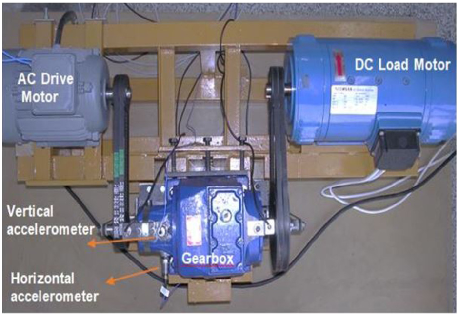
Using a resistor bank, the DC motor load was adjusted to four different levels. The first of these load conditions represents the no-load condition and is referred to as 0% load. The remaining load conditions in the gearbox correspond to 33%, 66%, and 100% of the maximum power of the DC load motor, respectively. Furthermore, a speed controller for the AC drive motor was employed to enable the gearbox to operate within the speed range of 0 to 3000 rpm. 43
Two PCB 352A76 type accelerometers were employed within a frequency range of 5–16,000 Hz to obtain the vibration signals generated by the gears. The accelerometers were placed at right angles to each other in the input shaft bearing housings as shown in Figure 1. The raw vibration data acquired from the accelerometers were sampled at 15 kHz and recorded on a computer using a data acquisition system and LabVIEW 7.0 software of National Instruments.
When there is angular misalignment in the gears, the surface contact stress along the face width of the mating gear teeth cannot be uniform. In this case, the distributed pitting fault, one of the gear failures that may occur in the future, is most likely to begin on the tooth surfaces where contact stresses greater than allowed are experienced.
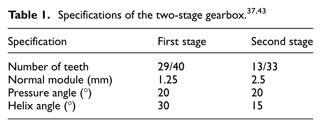
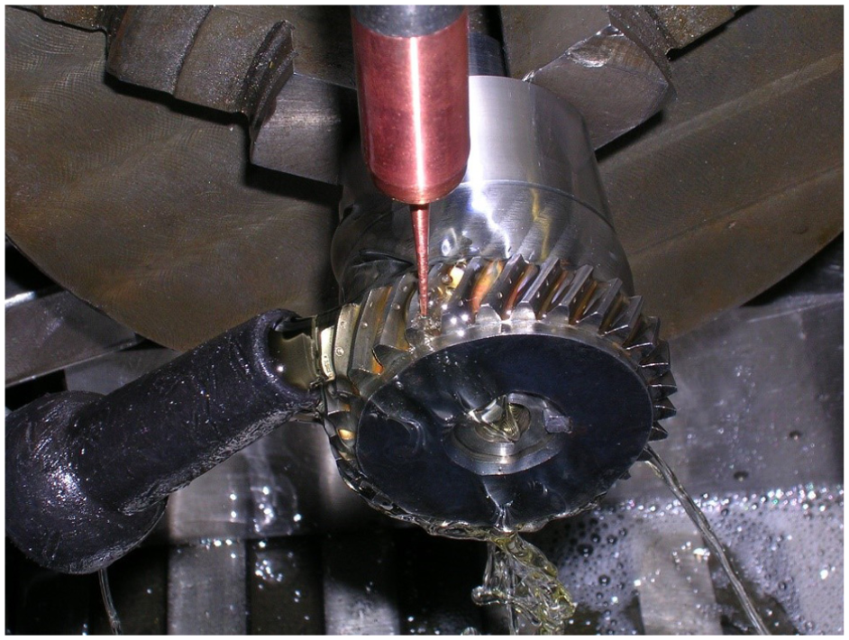
All distributed pitting faults were simulated in all teeth of the pinion gear using an electro-erosion machine, as shown in Figure 2; first, a circular pit, whose diameter and depth are approximately 0.7 and 0.1 mm, respectively, occurred on the surfaces of the tooth as shown in Figure 3(b). Subsequently, to represent the advancement of distributed pitting faults assumed to be caused by the presence of angular misalignment, the number of pits was increased as shown in Figure 3(c), (d), and (e).
Formation of distributed pitting failure on gear tooth surfaces using an electro-erosion machine. 43
The speed of the pinion gear is 2678 rpm, which gives a fundamental tooth meshing frequency of 1294 Hz for the first stage and 420.7 Hz for the second stage. Both vibration and positioning signals (inductive sensor) were sampled at 15 kHz. The raw vibration data were recorded continuously over 1337 pinion rotations.
Figure 4 presents the time and frequency domain representations of the vibration signals obtained from gears with four different types of distributed pitting and a healthy gear. The gearbox was disassembled and reassembled each time to simulate the distributed pitting fault on the tooth surfaces of the pinion gear. Due to this situation and manufacturing errors, a modulation that exhibits itself as repetitive fluctuations for each pinion rotation may have occurred.
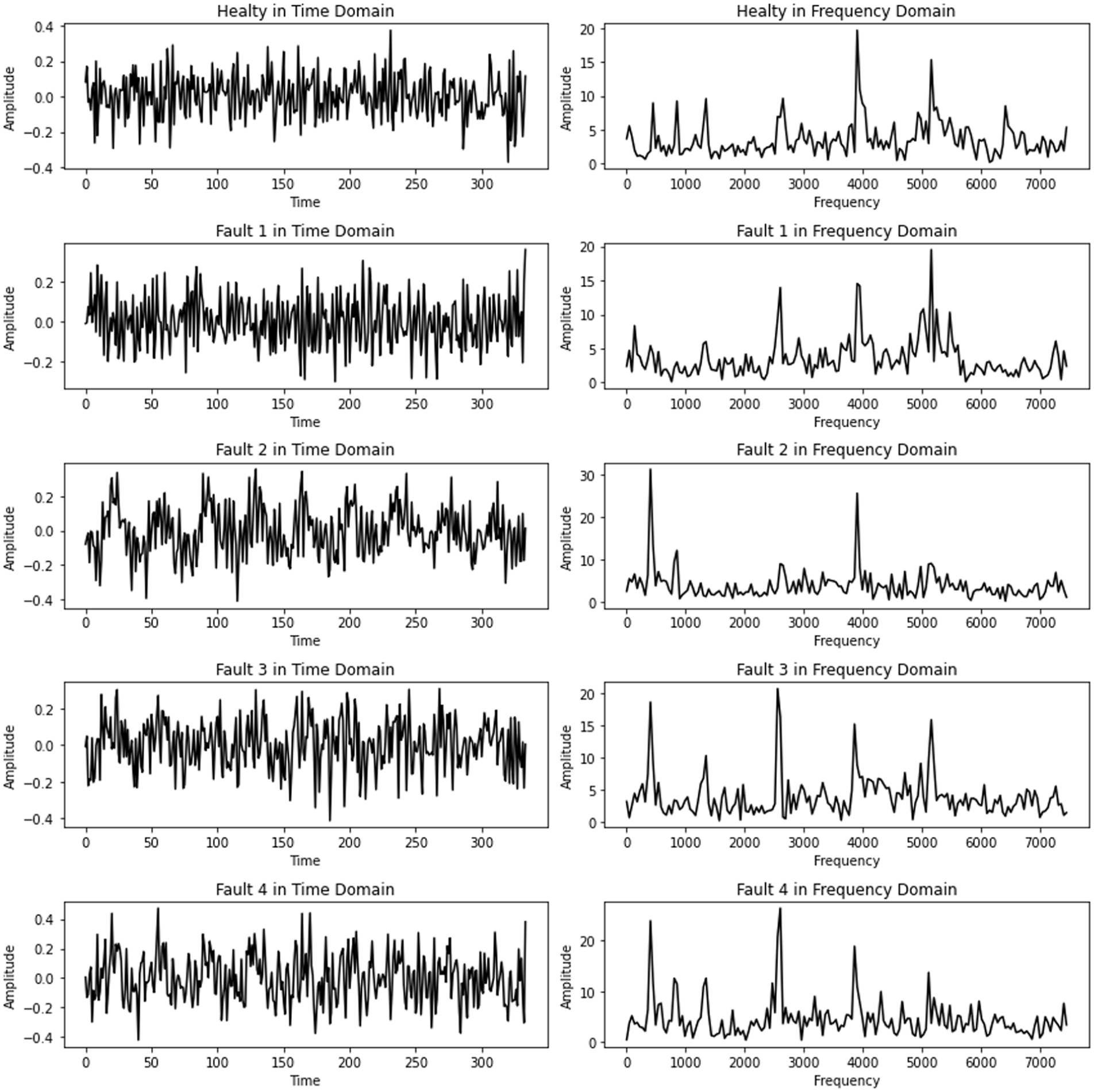
Raw vibration acceleration signals (A1 accelerometer) detected from the gearbox with distributed pitting and their corresponding spectra. 37
It is clear from Figure 4 that the vibration acceleration signals are similar, making it difficult to determine whether a distributed pitting fault exists or is developing. In particular, it has been shown in previous studies that advanced signal processing methods and computational load are needed for the early detection of distributed pitting damage and the evaluation of their severity.2,44–46
Dataset
The dataset includes five distinct classes: four representing different levels of pitting fault severity and one representing the healthy gear condition. The faults in the dataset are labeled as Fault 1, Fault 2, Fault 3, and Fault 4, and these labels directly correspond to the severity levels of the respective faults. Each class comprises data from three data channels: horizontal acceleration sensor data, vertical acceleration sensor data, and encoder output data. The encoder output data is used to determine the full-tour rotation of the gear. The full-tour rotation information was used to divide the horizontal and vertical sensor data into discrete windows for each rotation cycle. Consequently, each class was represented by 1337 data series, comprising 334 data points. As in Hizarcı et al., 46 the time series were filtered to remove noise between 1000 and 5400 Hz. This filtering step was applied to reduce high-frequency noise and improve signal consistency prior to model development.
Analyzing collected data using time-series methods offers significant advantages, particularly when examining frequency components and investigating signal dynamics. 47 Nevertheless, the remarkable effectiveness of image processing techniques within deep learning frameworks has highlighted the need to enhance feature richness by transforming temporal data into 2D representations. Therefore, the capabilities of deep learning algorithms can be exploited by creating images from existing data.48,49 Two different approaches were used to transform the vibration data into images.
In the first approach, the Morlet wavelet was used as the mother wavelet transform to generate scalogram images. The Morlet wavelet is a highly effective function that provides high accuracy in time–frequency analysis and enables the localization of signals. 50 The scale value is set in the range 1–20 for more precise separation of high and low frequency components. The scalogram images reflect the time–frequency distribution of the signal in detail and provide a rich and informative data source for deep learning models. This is particularly useful for capturing the dynamic characteristics of signals and helping to improve classification performance.
An alternative approach involves sequentially concatenating x-axis and y-axis accelerometer readings into a 2D matrix. 51 For each rotational movement instance, 334 data points from the x-axis are paired with an equal number of y-axis measurements, forming a combined vector of 668 temporal samples. To align with standard image-processing requirements, the dataset undergoes zero-padding by appending eight null values, yielding a 676-element vector. This adjusted sequence is subsequently reshaped into a 26 × 26 pixel matrix, ensuring square dimensionality for compatibility with CNN architectures commonly used in image-based deep learning frameworks. Figures 5 and 6 were created to provide a visual overview of the datasets.
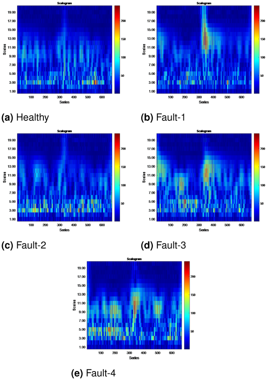
Scalogram-based representations of different fault conditions: (a) Healthy, (b) Fault 1, (c) Fault 2, (d) Fault 3, and (e) Fault 4.
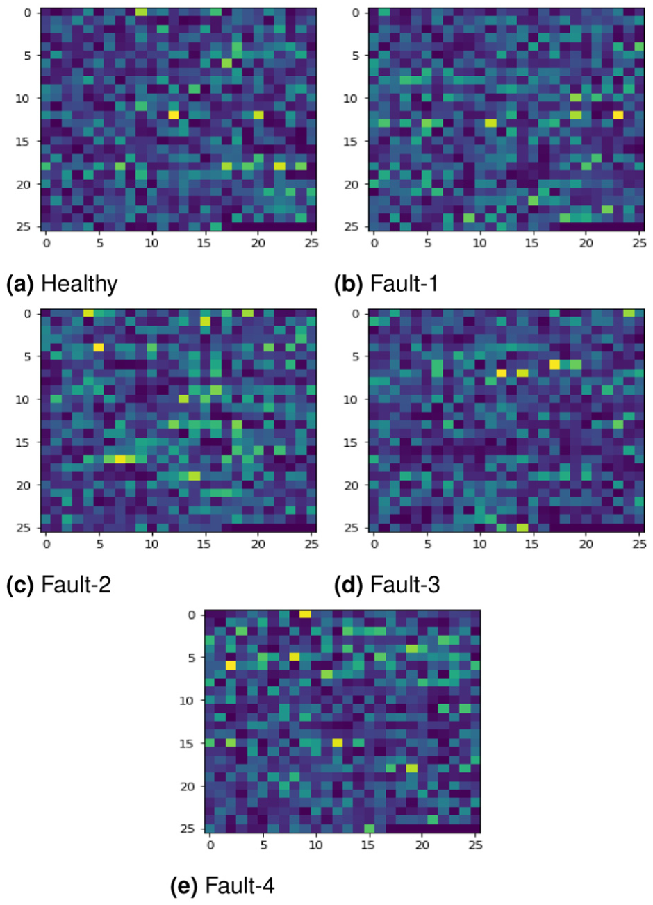
Data matrix representations of different fault conditions: (a) Healthy, (b) Fault 1, (c) Fault 2, (d) Fault 3, and (e) Fault 4.
Methodology
This study presents a methodology for the detection and severity classification of distributed pitting faults in a two-stage industrial helical gearbox. Because distributed pitting gives rise to complex and overlapping vibration responses, the diagnosis task is generally more challenging than that of more localized fault signatures. To examine this problem from different perspectives, the acquired vibration signals were represented in three forms: 1D time-domain signals, 26 × 26 data-matrix images, and 224 × 224 time–frequency scalograms.
To obtain a reliable assessment of performance, all closed-set classification experiments were conducted using a chronological split of 60% for training, 10% for validation, and 30% for testing without random shuffling to reduce the risk of temporal data leakage. Unless otherwise stated, the reported neural-model results were obtained using five predefined random seeds and are reported as mean ± standard deviation. Within this protocol, the validation subset was used for model selection and hyperparameter tuning, whereas the final reported results were obtained only on the held-out test subset.
The evaluated methods were grouped into four categories. First, handcrafted feature extraction combined with conventional classifiers was used to establish a baseline. Second, CNN models were applied according to the input format, including 1D-CNN for time-domain signals, LeNet-5 for the 26× 26 data matrices, and transfer learning models such as ResNet50, VGG-16, MobileNetV3-Large, and EfficientNet-B0 for the scalogram images. Third, AE-based models were used to learn compact latent representations from both 1D and 2D inputs. Finally, VAEs were evaluated as probabilistic alternatives to standard AEs, with the expectation that their latent-space structure could better capture the gradual and overlapping characteristics of distributed pitting signals.
Feature extraction
The feature extraction process involves selecting informative features that effectively represent the dataset. The features were evaluated and extracted using MATLAB’s Diagnostic Feature Designer tool, 52 after which a support vector machine (SVM) was used for classification. The extracted features include root mean square (RMS), mean, standard deviation, skewness, peak, signal-to-noise and distortion ratio (SINAD), signal-to-noise ratio (SNR), shape factor, kurtosis, clearance factor, impulse factor, crest factor, and total harmonic distortion (THD). 53 The extracted features characterize various statistical and signal properties: RMS represents the signal’s energy by measuring the square root of the average squared values, while the mean indicates the average signal level, and standard deviation reflects the degree of variation. Skewness describes the asymmetry of the signal distribution, peak value identifies the maximum amplitude, whereas SINAD and SNR provide measures related to signal clarity. The shape factor reflects the waveform shape by relating the RMS to the average value. Kurtosis measures the heaviness of the distribution tails, indicating outliers, while clearance factor, impulse factor, and crest factor, respectively, highlight fault-related characteristics by comparing peak values to different average or RMS measures. Finally, THD quantifies the distortion caused by harmonic frequencies relative to the fundamental signal component. Together, these features provide a conventional statistical description of the signal and serve as a baseline for comparison with the deep learning-based approaches.
Convolutional neural network
A CNN, which is a type of feedforward neural network, is capable of automatically extracting features from datasets through its convolutional structures. 54 The standard CNN architecture consists of several key layers: input, convolution, pooling, fully connected, and output layers.55,56 The convolutional layer applies multiple filters to these images, allowing the extraction of numerous features that are then transformed into feature maps. An activation function is then applied to introduce nonlinearity into the convolutional layer, which is essential to increase the learning capacity of the network. The pooling layer then reduces the spatial dimensions of the feature maps and the number of parameters, thereby improving computational efficiency. Although there are different types of pooling layers, this study uses max-pooling, a widely used technique that preserves the structural information of images. 57 The fully connected layer then consolidates the extracted features into a feature vector. Finally, the output layer maps this feature vector to class probabilities and determines the classification result. 58 The CNN models employed in this study can be categorized into 1D and 2D architectures, which are detailed below.
One-dimensional convolutional neural network
Specifically designed for 1D data, 1D-CNN employ kernels that slide along a single dimension, unlike traditional CNNs, which use two spatial dimensions. Recognizing the efficacy of 1D-CNN in processing 1D signals,59,60 to evaluate the performance of 1D-CNN in our dataset, we developed 12 distinct model architectures by hyperparameter tuning. The optimized hyperparameters include the number of convolutional layers, kernel size, pooling layer size, and the number of filters. These ranges were selected to cover shallow-to-moderate architectures that were compatible with the dataset size and signal length, while avoiding unnecessarily large models that could increase overfitting risk and computational cost. A total of twelve different 1D-CNN models were applied on vibration data obtained under different load conditions (no load, 33%, 66%, and full load).
Two-dimensional convolutional neural network
2D-CNNs are widely used for processing image-based data because they can detect spatial and hierarchical patterns in 2D inputs. 2D-CNNs offer a significant advantage in that they can effectively learn complex visual features from images. This study used 2D-CNNs to analyze visual representations derived from vibration signals. Specifically, transfer learning was used to train ResNet50 and VGG-16 models, as well as MobileNetV3 and EfficientNet-B0, with scalogram images, which offer time–frequency representations of the signals. In parallel, the LeNet-5 model was also trained on the data matrix image set to enable a comparative evaluation with a simpler architecture.
Transfer learning with ResNet50 and VGG-16 models, MobileNetV3, and EfficientNet-B0
ResNet50 and VGG-16 models, which are among the most popular choices due to their high performance rates, are used for the classification of distributed pitting faults. ResNet50 is a deep CNN comprising 50 layers, initially proposed by Microsoft Research Asia in 2015.61,62 The most significant distinction between ResNet50 and other networks is its implementation of residual connections, which effectively addresses the issue of gradient vanishing and enables the training of dense models. 63
The VGG-16 architecture represents a deep CNN, as outlined in the study by Simonyan and Zisserman. 64 The use of compact 3 × 3 filters in the convolution layers allows for a narrow detection area while allowing the addition of more layers and the use of a deeper network. It has demonstrated state-of-the-art performance in numerous image recognition benchmarks, including the ImageNet large-scale visual recognition challenge held in 2014.
In addition to these widely used architectures, MobileNetV3 65 and EfficientNet-B0 66 were also included in the comparative evaluation. These models were selected because they provide more computationally efficient alternatives while maintaining strong image classification capability, making them relevant for practical fault diagnosis settings.
The transfer learning method is used to reduce the dependency of the evaluated 2D-CNN models on large amounts of task-specific labeled data. This method uses knowledge from models that have been pre-trained on large datasets (e.g., ImageNet) to solve related problems,67,68 which is particularly useful in industrial settings where labeled fault data are often limited. 69
LeNet-5 model
LeNet-5 represents a groundbreaking advance in the domain of CNNs. It was developed by Yann LeCun and his team in 1998. 70 The LeNet-5 network comprises seven layers, including two convolutional layers, two subsampling layers, and three fully connected layers. 71 The standard LeNet-5 architecture includes an input layer with dimensions of 32× 32 or 28× 28. As the image set has dimensions of 26 × 26, modifications have been implemented in certain layers of the network architecture to accommodate this input size. The architecture of the modified LeNet-5 is shown in Figure 7.
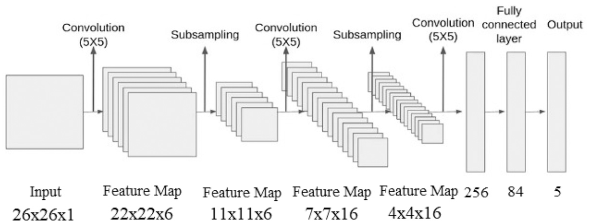
Modified LeNet-5 architecture.
Autoencoder
AEs, which were first introduced in the mid-1980s by Hinton et al.72,73 within the Parallel Distributed Processing (PDP) framework, aim to compress high-dimensional input data into a low-dimensional representation, known as the latent space, while minimizing information loss. 74 The reduction in information loss results in minimization of distortion between the input and output data. Consequently, high-dimensional images can be represented using the latent space. The latent space representation learned by the AE can serve as a feature vector for subsequent classifier algorithms. This approach allows classifiers to be trained with low-dimensional representative values of high-dimensional images. In this article, both 1D and 2D-AE architectures were employed depending on the structure of the input data. While 1D-AEs are preferred for raw time-series signals, 2D-AEs are more suitable for visual representations such as images.
One-dimensional autoencoder
One-dimensional AEs are specifically designed to process sequential data, making them particularly suitable for vibration signals recorded over time. Unlike 2D-AEs, which operate on spatially structured image data, 1D-AEs preserve the temporal ordering of the input, enabling the model to learn patterns inherent in time-dependent sequences. In this study, horizontal and vertical vibration signals were concatenated and used as inputs to the 1D-AE model. The goal was to obtain compact latent representations that could be used to train classifiers more efficiently. The properties of 1D-AE are given in Table 2. 1D-AEs are particularly useful in applications where preserving the sequential structure of the data is critical, such as time-series analysis.75,76 In this approach, the latent space is reduced to 50-dimensional data, and the aim is to train the classifier algorithms with these latent space values.
1D-AE architecture.
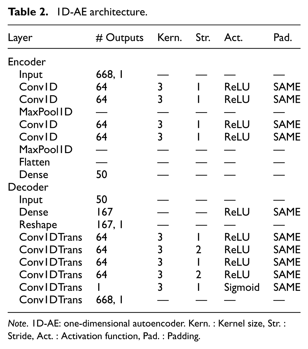
Note. 1D-AE: one-dimensional autoencoder. Kern. : Kernel size, Str. : Stride, Act. : Activation function, Pad. : Padding.
Two-dimensional autoencoder
2D-AEs are widely used for image-based data, where spatial structure and local dependencies carry essential information. In the context of this study, 2D-AEs were trained on scalogram and data matrix images derived from vibration signals. These models aim to compress high-dimensional visual representations into compact latent vectors while preserving important structural features relevant for fault detection. Due to the varying image sizes employed in the study, two different architectures are presented in Tables 3 and 4, each optimized for the specific type of input image.
2D-AE architecture for scalogram images.
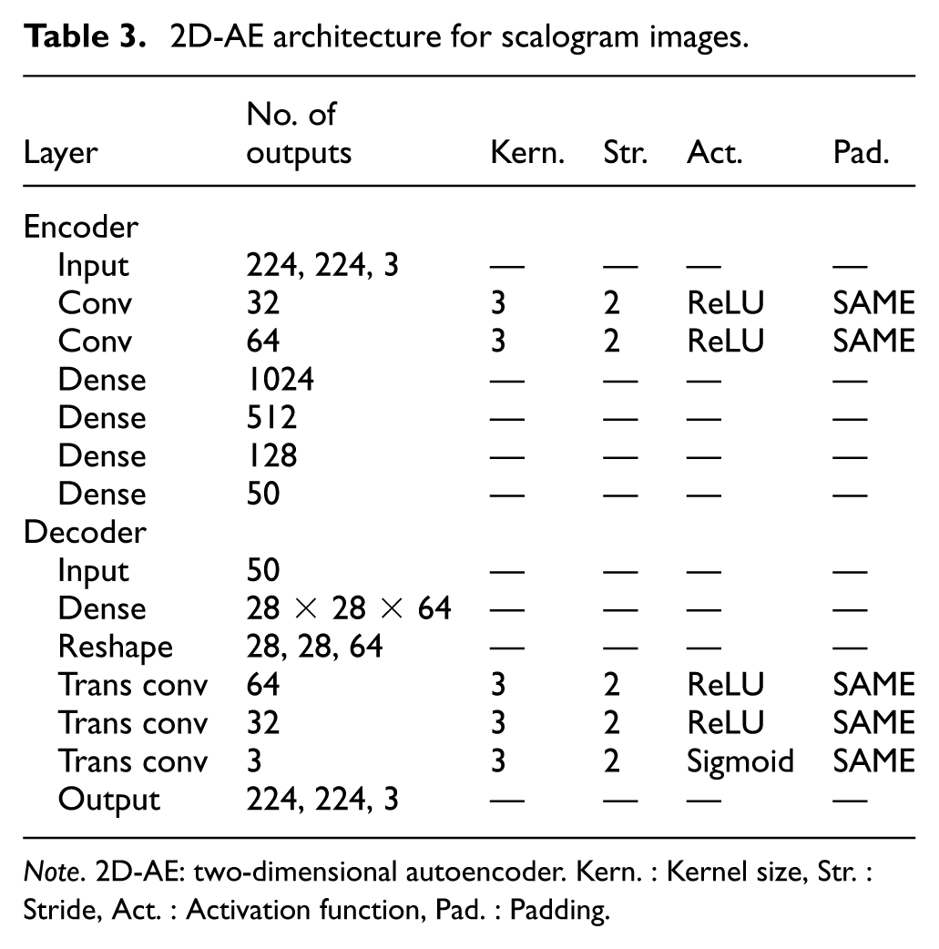
Note. 2D-AE: two-dimensional autoencoder. Kern. : Kernel size, Str. : Stride, Act. : Activation function, Pad. : Padding.
2D-AE architecture for data matrix images.
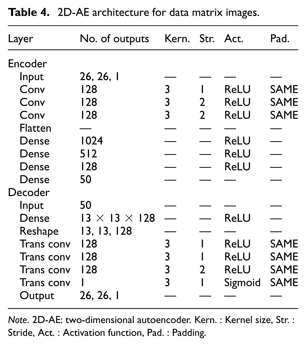
Note. 2D-AE: two-dimensional autoencoder. Kern. : Kernel size, Str. : Stride, Act. : Activation function, Pad. : Padding.
Variational autoencoders
VAEs represent a specific subcategory of AEs that adopt a probabilistic methodology in the encoding process. In contrast to a classical AE, a VAE compresses the input data as a probability distribution that includes mean and variance. 77 This enables the VAE to learn a distribution over the latent space and to capture the statistical structure of the data. 78 As with the classical AE approach, the latent space and probability distribution obtained in the VAE approach can be employed as a feature for the aforementioned classifier algorithms. The block diagram representation of the general VAE structure is presented in Figure 8.
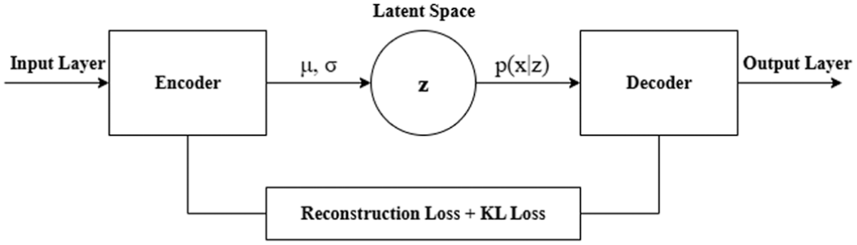
VAE architecture. 79 VAE: variational autoencoder.
In this study, VAE architectures were developed for both 1D and 2D input data, extending the corresponding AE structures by incorporating the reparameterization trick.
One-dimensional variational autoencoder
The 1D-VAE structure is derived from the classical 1D-AE model and is tailored for time-series data such as vibration signals. By modeling the latent space as a distribution rather than a point estimate, 1D-VAEs enable more robust and expressive feature extraction from sequential inputs. The 1D VAE adopts the same architecture as the 1D AE presented in Table 2; the main difference lies in the use of the reparameterization trick to model the latent space probabilistically. In the context of 1D VAE, the latent space values encompass probabilistic distribution information, including the mean and variance.
Two-dimensional variational autoencoder
For image-based data, the 2D-VAE architecture builds upon the previously introduced 2D-AE structures designed for scalogram and data matrix images. The same convolutional and dense layers are preserved, while the encoder is modified to output both the mean and variance vectors for the latent variables. A common approach was used with AE architectures for different image sets, and the VAE architecture was created by adding the reparametrization trick to the architectures shown in Tables 3 and 4.
Following the formulation of the AE and VAE architectures, establishing a robust training framework is essential to ensure the reliability of the extracted features. To this end, hyperparameters were determined through targeted pilot studies rather than exhaustive grid searches. This approach efficiently addresses the structural complexity of both 1D and 2D data while preventing overfitting. The VAE architectures were intentionally designed as direct extensions of the AEs. This ensures a fair, controlled baseline for evaluating probabilistic regularization.
The latent dimensionality was set to
Training hyperparameters were also empirically established. The Adam optimizer, with a learning rate of
Results and discussion
The performance of the methods used in this study is evaluated in this section. First, results obtained from approaches utilizing vibration signals as 1D time-series data are presented, including handcrafted feature extraction combined with classifiers, various CNN architectures, AEs, and VAEs. The performance of the methods applied to vibration signals transformed into images using two different techniques is then detailed. For the scalogram image dataset, transfer learning is performed using pre-trained ResNet50 and VGG-16 models, alongside AEs and VAEs. Finally, the performance of LeNet-5, AEs, and VAEs is evaluated on the 26 × 26 pixel image dataset.
1D-dataset: Vibration signals
This section addresses the performance of machine learning methods applied to vibration signal data obtained from accelerometers. First, the approach of extracting handcrafted statistical features and performing classification is presented. Subsequently, CNN, AE, and VAE-based representation learning methods were evaluated and compared.
Handcrafted feature extraction and classification
In the field of signal analysis, novel methodologies are continuously being developed for the analysis of 1D signals. However, statistical signal analysis methods remain prevalent as a baseline. The present study involves an analysis of the 13 features referenced in the “Methodology” section. These features were ranked according to their discriminative importance using a one-way analysis of variance test. To this end, a series of studies were conducted using the most significant 2 features, 4 features, 7 features, 12 features, and all 13 features. The results demonstrated that performance, represented by accuracy, was 49.75% for the two most significant features, 61.64% for four features, 67.11% for seven features, 66.87% for twelve features, and 66.62% when all features were included. It was observed that the highest performance was obtained by using the most important seven features, and the confusion matrix is presented in Table 5. The seven-feature subset consisted of RMS, Mean, Standard Deviation, Skewness, Peak, SNR, and SINAD. Including additional features beyond this point led to a slight decrease in performance. The standard deviation across the five runs was observed to be ± 0.00, which is consistent with the deterministic behavior of the SVM classifier under a fixed chronological data split.
Confusion matrix with seven optimal handcrafted features for load condition 0%.
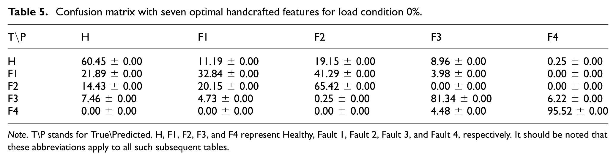
Note. T\P stands for True\Predicted. H, F1, F2, F3, and F4 represent Healthy, Fault 1, Fault 2, Fault 3, and Fault 4, respectively. It should be noted that these abbreviations apply to all such subsequent tables.
For reference, the handcrafted feature extraction and SVM pipeline was also evaluated computationally. The total training time was 0.2226 s, and the end-to-end inference time was 0.5561 ms per sample, including feature extraction and SVM prediction. The peak memory usage during inference was 1.0917 MB of RAM. As shown in Table 5, the handcrafted feature-based approach still struggles to distinguish between some degradation states, with Fault 1 being most frequently confused with Fault 2 and Healthy. This suggests that manually extracted statistical features alone are not sufficient to capture the more complex degradation patterns in the vibration signals.
One-dimensional convolutional neural network
1D-CNN models with varying architectures were constructed by modifying the number of convolution layers, the number of filters, the pooling size, and the kernel size. The impact of these modified parameters on the fault detection performance of the models was examined. A total of twelve different 1D-CNN models were applied on vibration data obtained under different load conditions (no load, 33%, 66%, and full load), and their performances were evaluated over five predefined random seeds. Table 6 provides a comprehensive overview of the parameter values and the mean accuracy values of the models. Models with 1, 2, and 3 convolutional layers showed comparable accuracy rates, with a single convolutional layer providing the best compromise between accuracy and computational efficiency. The kernel size variations revealed that smaller kernels were generally sufficient, while larger pooling layers tended to reduce performance because they caused greater feature loss. Finally, the number of filters showed that 16 filters provided the optimal compromise between accuracy and computational cost, achieving robust performance with lower computational demand than wider models. Therefore, it is concluded that the optimization of these parameters is of crucial importance to maintain high accuracy while minimizing complexity in fault detection tasks. As a result of these observations, model 1 was selected as the final configuration because it provided the most favorable overall trade-off between accuracy and computational efficiency. The confusion matrix of the best model for no load condition is given in Table 7. The model achieved an overall accuracy of 99.40%.
Accuracies of 1D-CNN models under varying load conditions and architectural parameters.
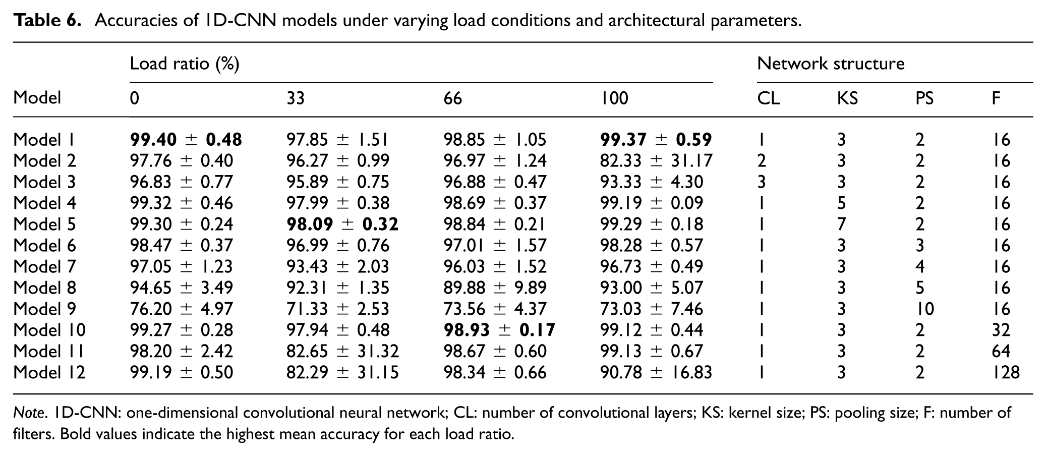
Note. 1D-CNN: one-dimensional convolutional neural network; CL: number of convolutional layers; KS: kernel size; PS: pooling size; F: number of filters. Bold values indicate the highest mean accuracy for each load ratio.
Confusion matrix of 1D-CNN for load condition 0%.
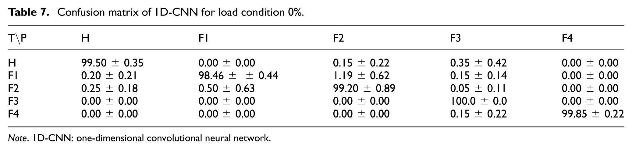
Note. 1D-CNN: one-dimensional convolutional neural network.
One-dimensional autoencoder
The performance of the 1D-AE approach applied to the analysis of 1D vibration signals is presented in Table 8. The overall accuracy was 96.25%. The main performance loss appears to arise from confusion between Fault 1 and Fault 2, together with the relatively lower and more variable recall of Fault 3.
Confusion matrix of 1D-AE for load condition 0%.
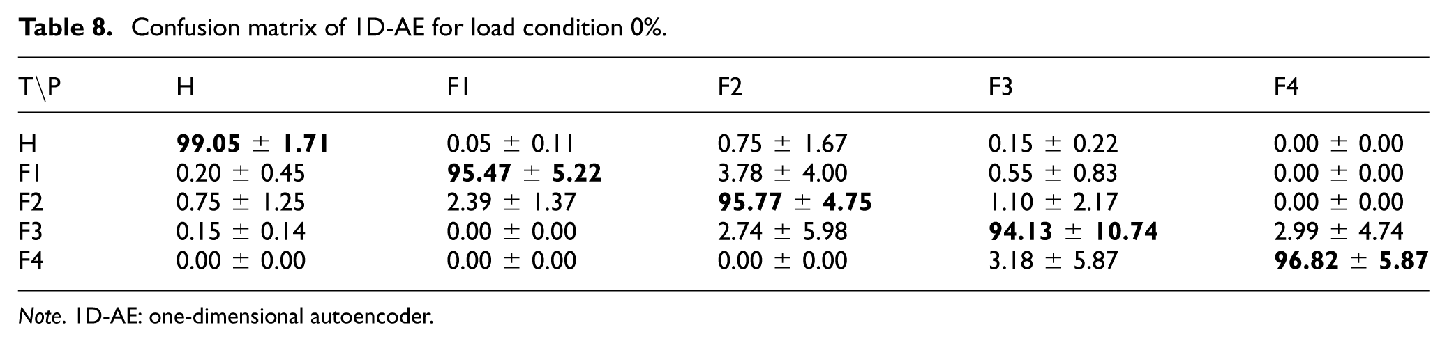
Note. 1D-AE: one-dimensional autoencoder.
One-dimensional variational autoencoder
Table 9 shows the performance of the 1D-VAE method, which adds a statistical approach to the 1D-AE method. The VAE model performs better than the AE model. Although the detection accuracy for the Fault 1 and Fault 2 classes was lower than for the other classes, this disparity was less significant compared to the 1D-AE method. The overall accuracy achieved by the 1D-VAE method was 98.96%.
Confusion matrix of 1D-VAE for load condition 0%.
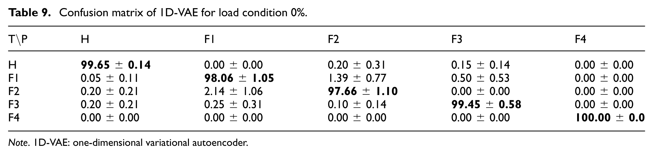
Note. 1D-VAE: one-dimensional variational autoencoder.
2D-dataset: 224 × 224 scalogram image
This section discusses the performance of machine learning methods using scalogram images obtained with the continuous wavelet transform applied to the vibration signal data. The methods described in the methodology section are presented sequentially.
ResNet50
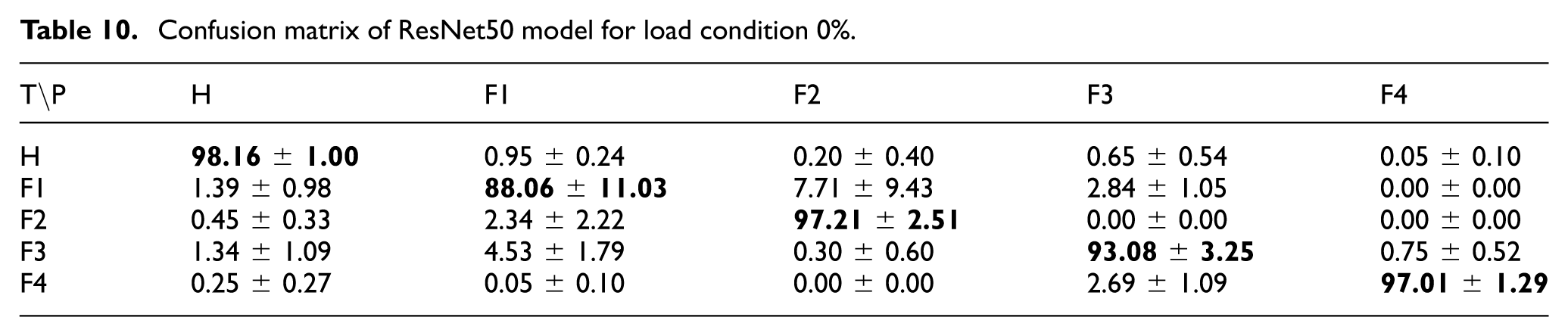
The ResNet50 model was employed to classify images of dimensions 224 × 224 using the transfer learning method. Evaluated over five predefined random seeds, the trained model exhibited the following mean accuracy rates and standard deviations for the five classes: “Healthy” (98.16 ± 1.00%), “Fault 1” (88.06 ± 11.03%), “Fault 2” (97.21 ± 2.51%), “Fault 3” (93.08 ± 3.25%), and “Fault 4” (97.01 ± 1.29%). In addition to the individual class accuracy rates mentioned above, the overall system performance was calculated, resulting in an accuracy rate of approximately 94.71%. The confusion matrix generated by the performance of the ResNet50 model under the 0% load condition is presented in Table 10.
Confusion matrix of ResNet50 model for load condition 0%.
VGG-16
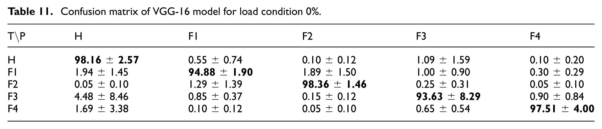
The VGG-16 model was evaluated under the 0% load condition. Across five random seeds, the model achieved mean class accuracies of 98.16 ± 2.57% for “Healthy,” 94.88 ± 1.90% for “Fault 1,” 98.36 ± 1.46% for “Fault 2,” 93.63 ± 8.29% for “Fault 3,” and 97.51 ± 4.00% for “Fault 4.” The overall average accuracy was 96.51%. The corresponding confusion matrix is presented in Table 11.
Confusion matrix of VGG-16 model for load condition 0%.
MobileNetV3
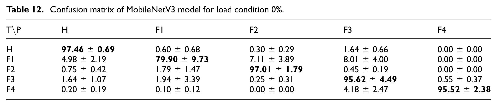
The MobileNetV3 model was evaluated under the 0% load condition. Across five random seeds, the model achieved mean class accuracies of 97.46 ± 0.69% for “Healthy,” 79.90 ± 9.73% for “Fault 1,” 97.01 ± 1.79% for “Fault 2,” 95.62 ± 4.49% for “Fault 3,” and 95.52 ± 2.38% for “Fault 4.” The overall average accuracy was 93.10%. The corresponding confusion matrix is presented in Table 12.
Confusion matrix of MobileNetV3 model for load condition 0%.
EfficientNet-B0
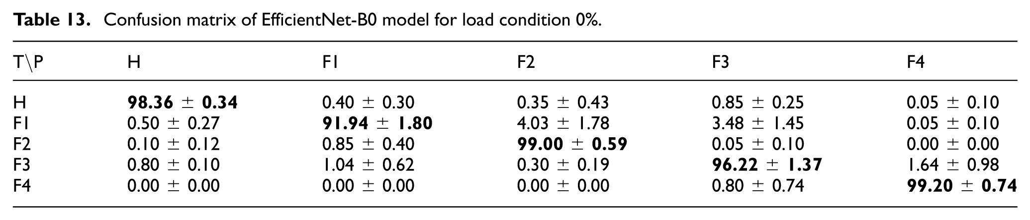
The EfficientNet-B0 model was evaluated under the 0% load condition. Across five random seeds, the model achieved mean class accuracies of 98.36 ± 0.34% for “Healthy,” 91.94 ± 1.80% for “Fault 1,” 99.00 ± 0.59% for “Fault 2,” 96.22 ± 1.37% for “Fault 3,” and 99.20 ± 0.74% for “Fault 4.” The overall average accuracy was 96.95%. The corresponding confusion matrix is presented in Table 13.
Confusion matrix of EfficientNet-B0 model for load condition 0%.
Two-dimensional autoencoder
For the 2D-AE approach based on scalogram images, the AE was trained on the training subset and then used to extract latent features from the training, validation, and test data. These latent representations were subsequently used for classification, and among the evaluated classifiers, the SVM yielded the best results, with the validation set used for hyperparameter tuning. Across five random seeds, the AE–SVM pipeline achieved mean class accuracies of 99.75 ± 0.27% for “Healthy,” 96.72 ± 0.19% for “Fault 1,” 98.31 ± 0.24% for “Fault 2,” 98.06 ± 0.43% for “Fault 3,” and 98.51 ± 0.31% for “Fault 4.” The overall average accuracy was 98.27%, and the corresponding confusion matrix under the 0% load condition is presented in Table 14.
Confusion matrix of 2D-AE model for load condition 0%.
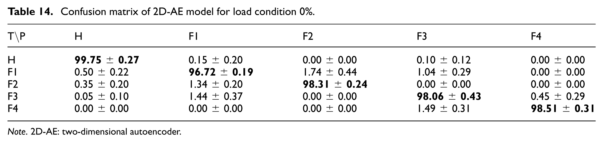
Note. 2D-AE: two-dimensional autoencoder.
Two-dimensional variational autoencoder
For the 2D VAE approach applied to 224 × 224 scalogram images, the VAE was trained on the training subset and then used to extract latent representations (
When evaluated on the unseen
Confusion matrix of VAE model for load condition 0%.
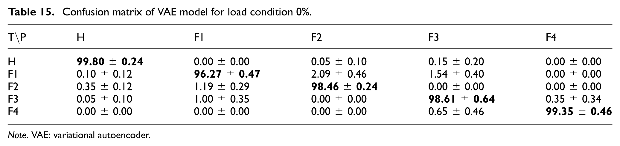
Note. VAE: variational autoencoder.
2D-dataset: 26 × 26 Data matrix
This section discusses the performance of machine learning methods using a 26× 26 image set generated with two-axis vibration signal data. Initially, the architecture of LeNet-5, a well-established deep learning model, is presented. This is followed by the performance of AE and VAE approaches, respectively.
LeNet-5
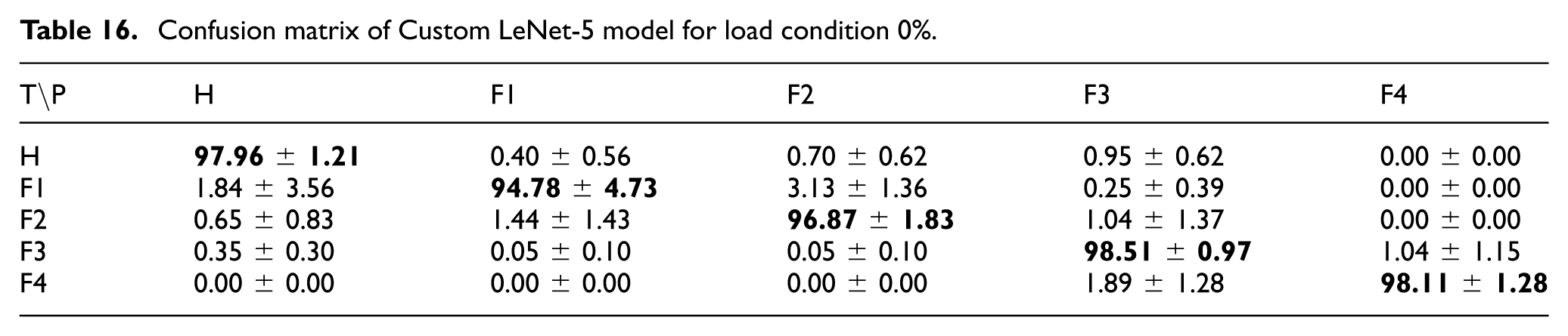
The custom LeNet-5 model, operating on 26 × 26 input images, was evaluated under the 0% load condition. Across five random seeds, the model achieved mean class accuracies of 97.96 ± 1.21% for “Healthy,” 94.78 ± 4.73% for “Fault 1,” 96.87 ± 1.83% for “Fault 2,” 98.51 ± 0.97% for “Fault 3,” and 98.11 ± 1.28% for “Fault 4.” The overall average accuracy was 97.24%. The corresponding confusion matrix for the Custom LeNet-5 model is presented in Table 16. Despite the reduced input size, the model maintained competitive classification performance.
Confusion matrix of Custom LeNet-5 model for load condition 0%.
Two-dimensional autoencoder
The 2D-AE approach was also applied to the 26× 26 data matrix images. The AE was trained on the training subset and used to construct latent representations (
Confusion matrix of 2D-AE model for load condition 0%.
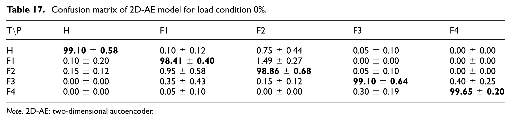
Note. 2D-AE: two-dimensional autoencoder.
Two-dimensional variational autoencoder
In the 2D-VAE approach, the same architecture as the corresponding AE was used for the 26 × 26 images. The VAE was trained on the training subset, and the resulting latent representations (
Confusion matrix of VAE model for load condition 0%.
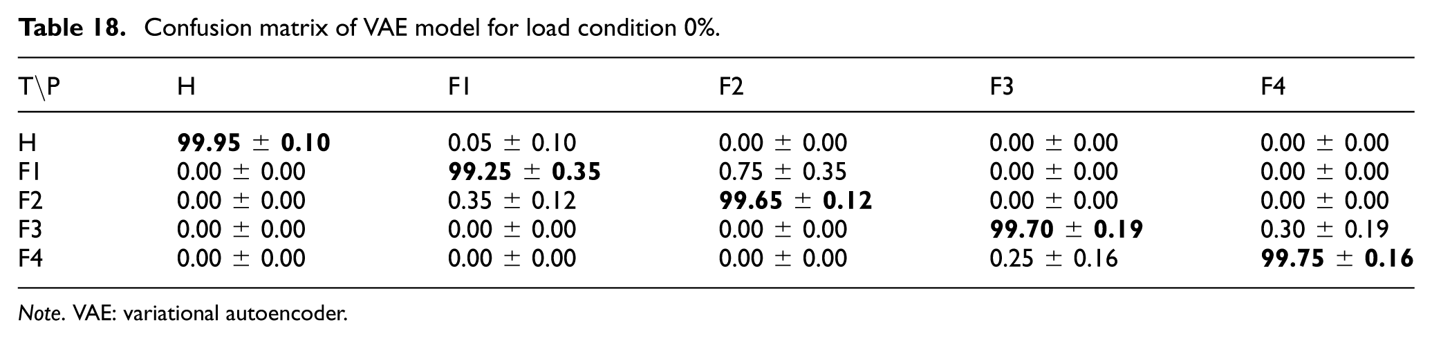
Note. VAE: variational autoencoder.
A comparative analysis of different input representations
The performance of the methods for three distinct input representations—1D time-series data, 224× 224 scalogram images, and 26× 26 data matrices—is summarized in Table 19 for the no-load (0%) condition. The results indicate that deep learning-based automatic feature extraction substantially outperformed traditional feature extraction and shallow learning (FESL) methods, which achieved an accuracy of 67.11 ± 0.00%. This finding highlights the difficulty of manually extracting discriminative features from complex vibration signals. Among the 1D input models, the 1D-CNN achieved 99.40 ± 0.48% accuracy. Although scalogram images are frequently used in the literature to capture time–frequency characteristics, the large pre-trained networks evaluated in this study did not exceed 97% accuracy. In contrast, the 2D-VAE model applied to the 26× 26 data matrices achieved the highest baseline accuracy of 99.66 ± 0.20%, indicating that effective latent representations can still be learned from substantially reduced input dimensions.
Overall performance comparison of the evaluated models under 0% load condition.
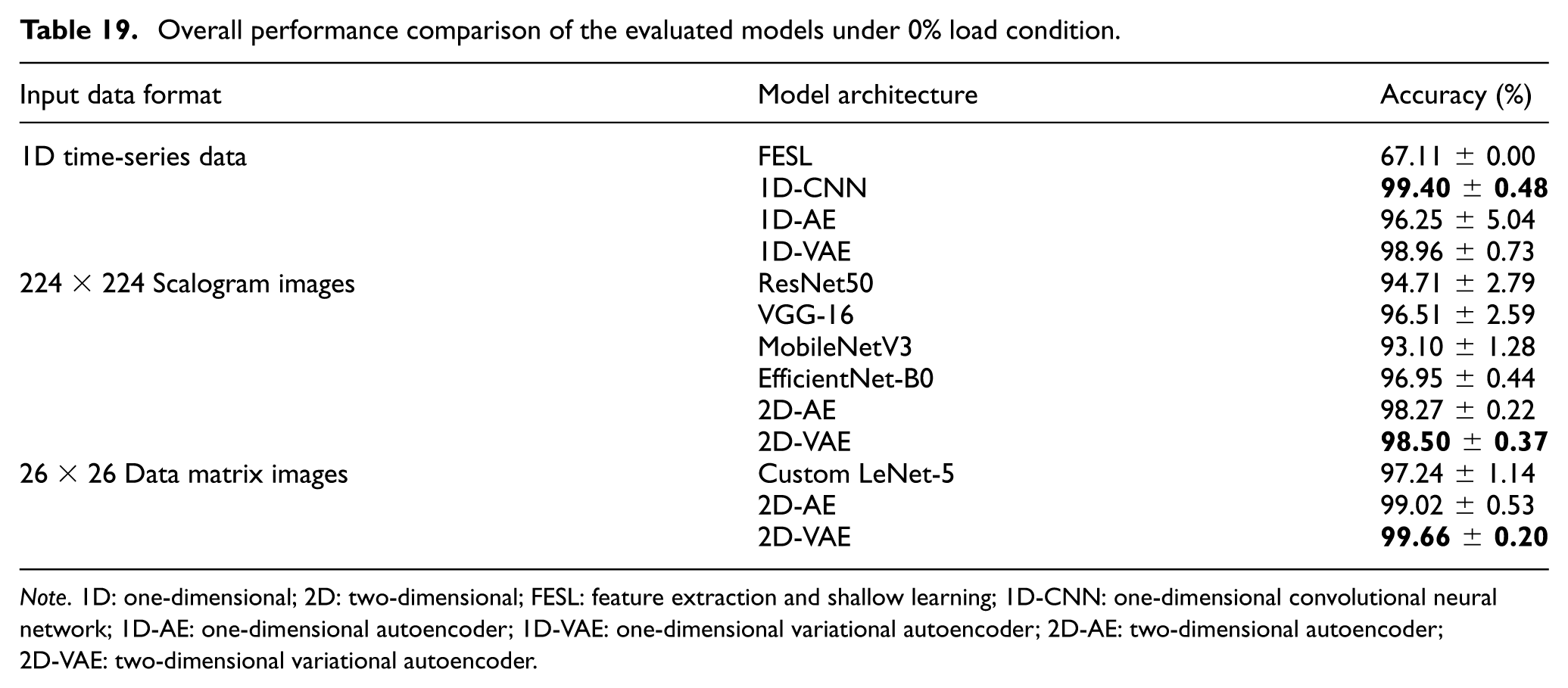
Note. 1D: one-dimensional; 2D: two-dimensional; FESL: feature extraction and shallow learning; 1D-CNN: one-dimensional convolutional neural network; 1D-AE: one-dimensional autoencoder; 1D-VAE: one-dimensional variational autoencoder; 2D-AE: two-dimensional autoencoder; 2D-VAE: two-dimensional variational autoencoder.
Methods that demonstrated a high degree of success were also applied to data collected under varying load conditions (0%, 33%, 66%, and 100%), as detailed in Tables 20, 21, 22, and 23, respectively. Finally, as illustrated in Table 24, the aggregated average accuracies across all load conditions are presented. It has been observed that the VAE architecture achieved the highest overall accuracy (
Performance under 0% load condition.
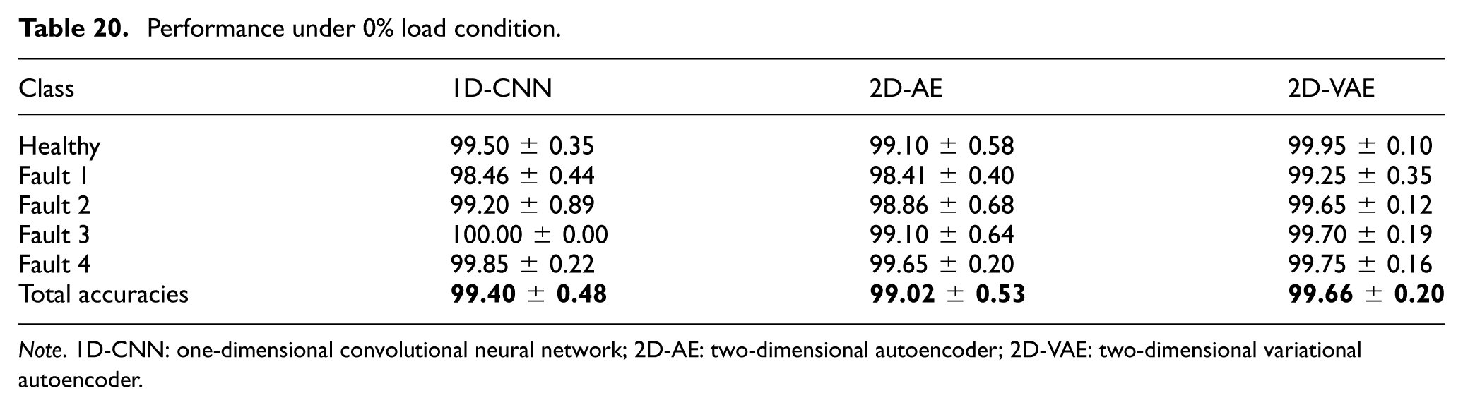
Note. 1D-CNN: one-dimensional convolutional neural network; 2D-AE: two-dimensional autoencoder; 2D-VAE: two-dimensional variational autoencoder.
Performance under 33% load condition.
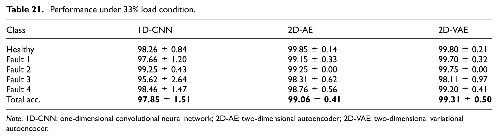
Note. 1D-CNN: one-dimensional convolutional neural network; 2D-AE: two-dimensional autoencoder; 2D-VAE: two-dimensional variational autoencoder.
Performance under 66% load condition.

Note. 1D-CNN: one-dimensional convolutional neural network; 2D-AE: two-dimensional autoencoder; 2D-VAE: two-dimensional variational autoencoder.
Performance under 100% load condition.
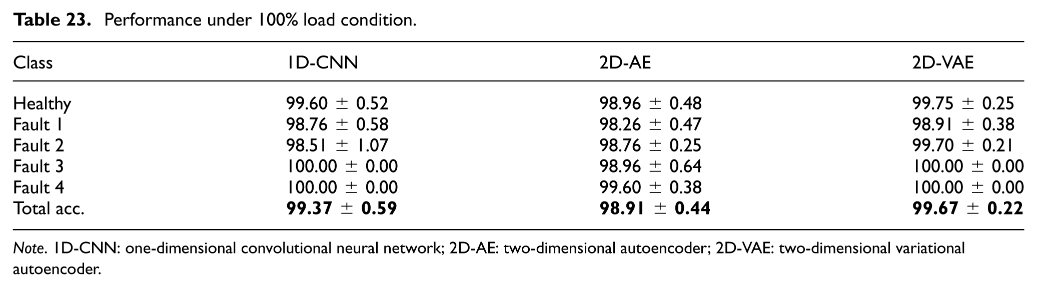
Note. 1D-CNN: one-dimensional convolutional neural network; 2D-AE: two-dimensional autoencoder; 2D-VAE: two-dimensional variational autoencoder.
Average accuracy from no-load to full-load condition.
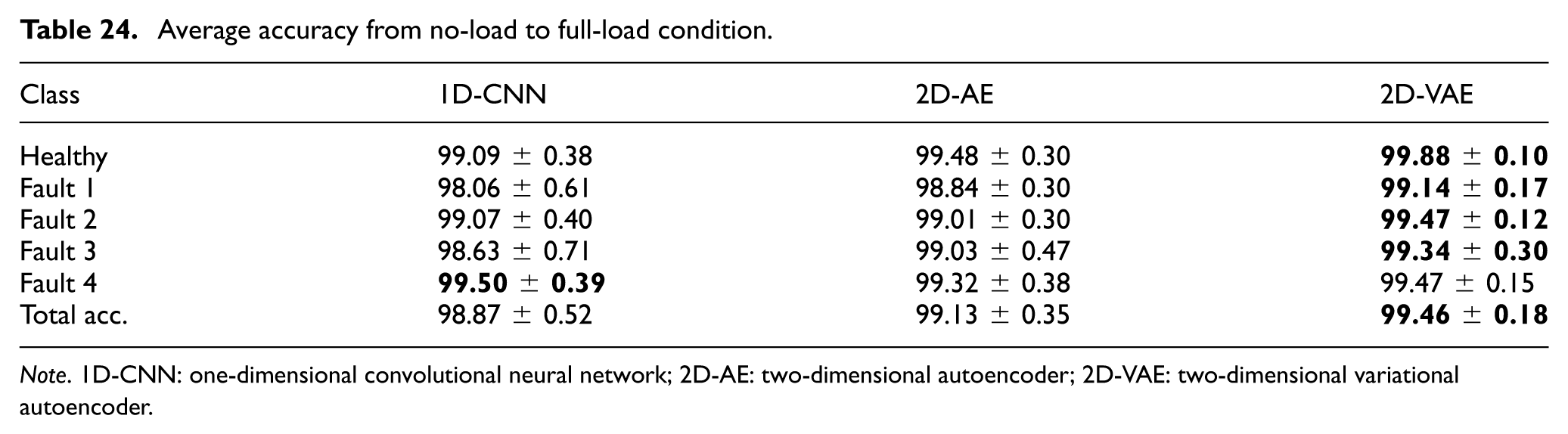
Note. 1D-CNN: one-dimensional convolutional neural network; 2D-AE: two-dimensional autoencoder; 2D-VAE: two-dimensional variational autoencoder.
Load-wise confusion matrix analysis of the three best-performing methods
Based on the comparative results in Table 19, the three best-performing methods (with a success rate above 99%) were further examined through their confusion matrices under different load conditions. This analysis provides a clearer view of how class-wise error patterns change with load.
For the 1D-CNN model, the confusion matrices under 33%, 66%, and 100% load conditions are presented in Tables 25 to 27. These results show that the model maintained strong performance across all evaluated loads, although the separation between adjacent fault classes changed slightly under transitional operating conditions.
Confusion matrix of 1D-CNN for load condition 33%.
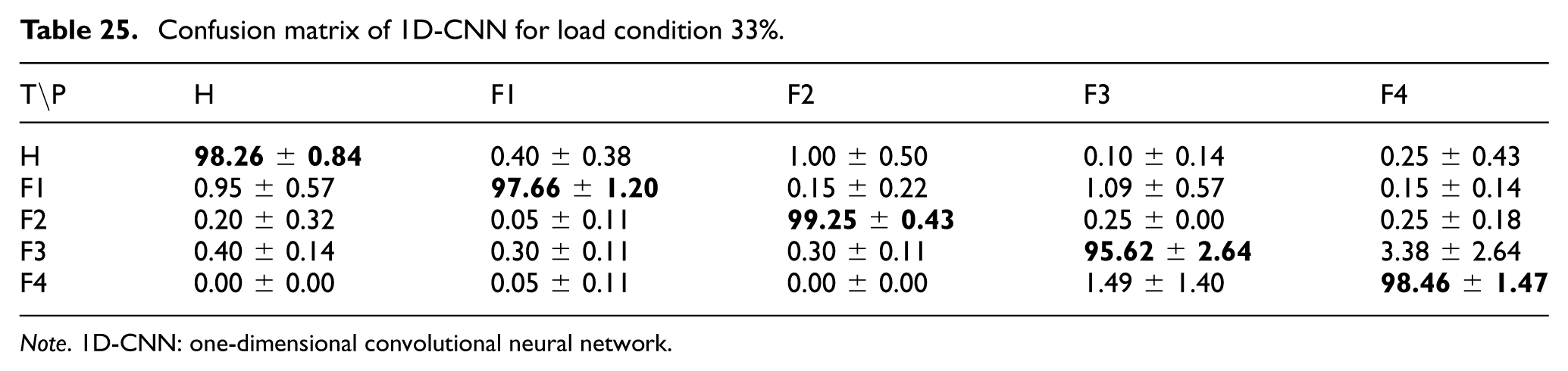
Note. 1D-CNN: one-dimensional convolutional neural network.
Confusion matrix of 1D-CNN for load condition 66%.
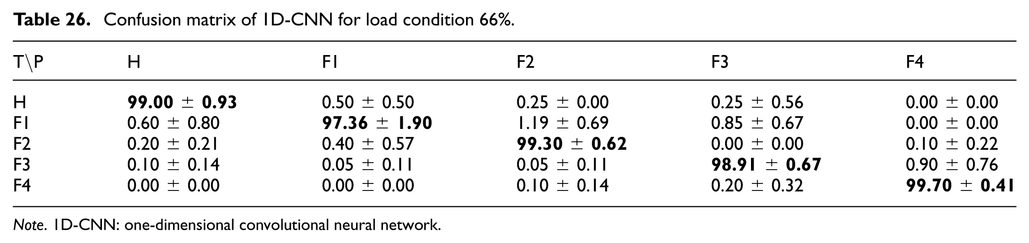
Note. 1D-CNN: one-dimensional convolutional neural network.
Confusion matrix of 1D-CNN for load condition 100%.
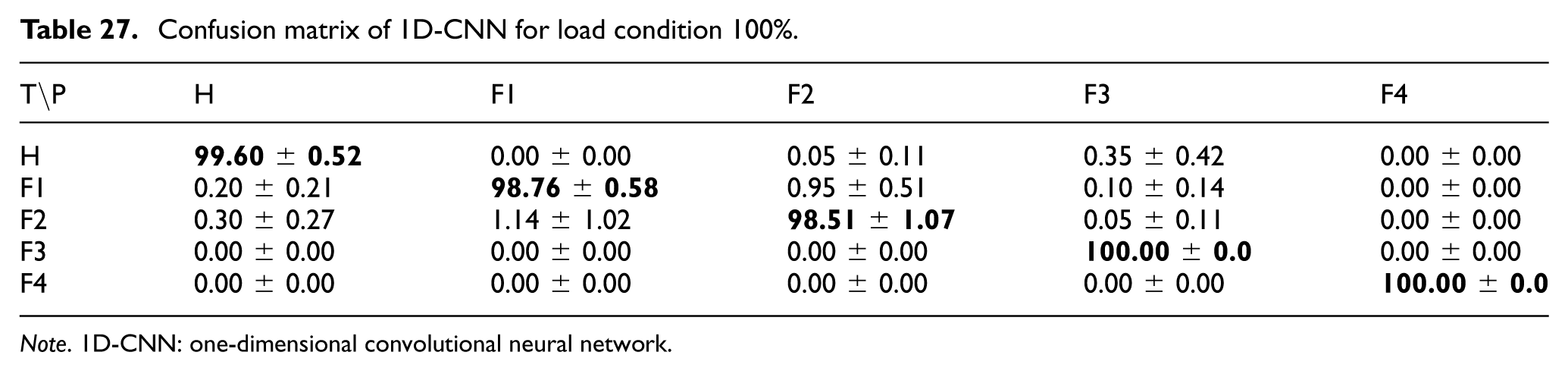
Note. 1D-CNN: one-dimensional convolutional neural network.
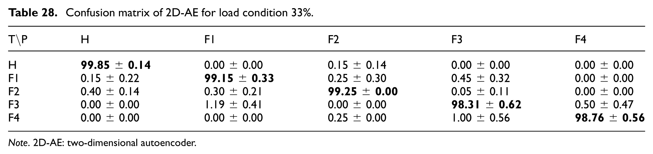
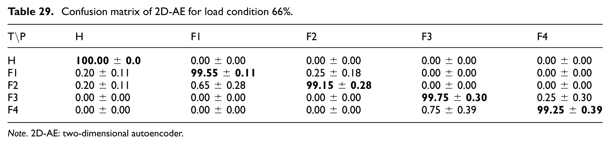
For the 2D-AE model based on 26× 26 data matrices, the corresponding confusion matrices under 33%, 66%, and 100% load conditions are reported in Tables 28 to 30. The results indicate that the model preserved high classification performance across load levels. At 33% load, the lowest class accuracy was 98.31 ± 0.62% for Fault 3. At 66% load, the Healthy class reached 100.00 ± 0.00%, and all fault classes exceeded 99% accuracy. At 100% load, the model remained close to its no-load performance, with the largest misclassification observed between Fault 1 and Fault 2 (1.59 ± 0.57%). Overall, these results suggest that the 2D-AE approach provides stable feature representations for the compressed data-matrix inputs across the evaluated load conditions.
Confusion matrix of 2D-AE for load condition 33%.
Note. 2D-AE: two-dimensional autoencoder.
Confusion matrix of 2D-AE for load condition 66%.
Note. 2D-AE: two-dimensional autoencoder.
Confusion matrix of 2D-AE for load condition 100%.
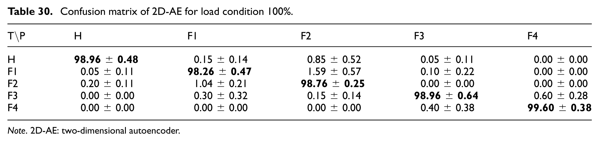
Note. 2D-AE: two-dimensional autoencoder.
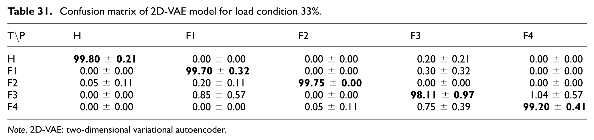
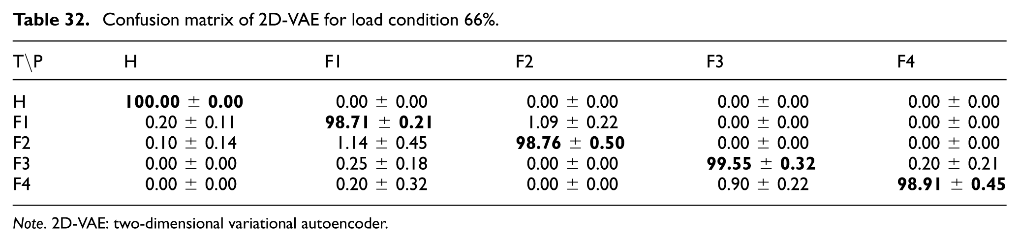
For the 2D-VAE model, the confusion matrices under 33%, 66%, and 100% load conditions are shown in Tables 31 to 33. The results indicate that the 2D-VAE maintained highly stable classification performance across all evaluated load conditions. At 33% load, the lowest class accuracy was 98.11 ± 0.97% for Fault 3, whereas at 66% load the Healthy class reached 100.00 ± 0.00%, and at 100% load both Fault 3 and Fault 4 were classified with 100.00 ± 0.00% accuracy. These results are consistent with the overall trends in Table 24 and suggest that the probabilistic latent representation remained robust under varying load levels.
Confusion matrix of 2D-VAE model for load condition 33%.
Note. 2D-VAE: two-dimensional variational autoencoder.
Confusion matrix of 2D-VAE for load condition 66%.
Note. 2D-VAE: two-dimensional variational autoencoder.
Confusion matrix of 2D-VAE for load condition 100%.
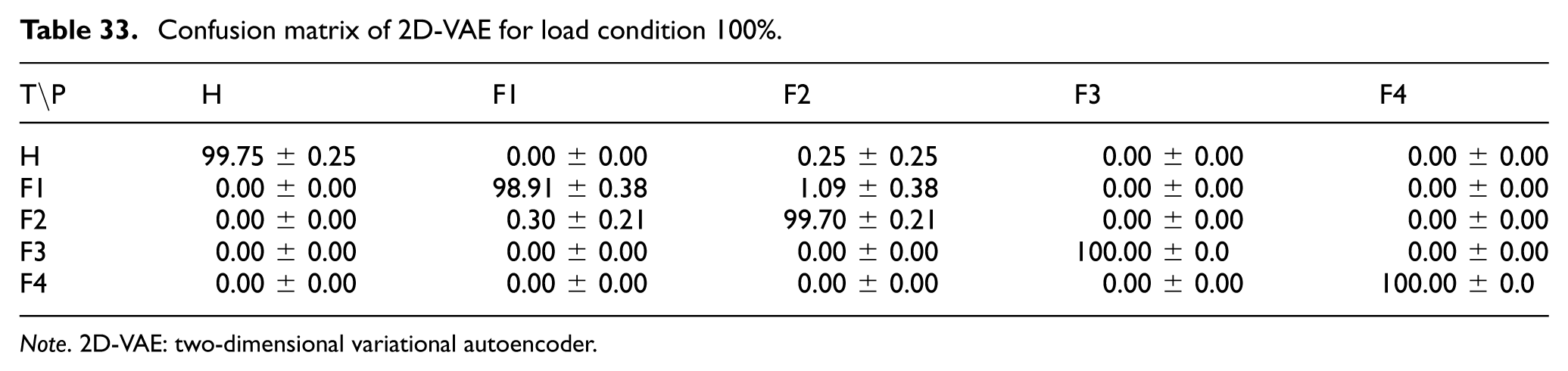
Note. 2D-VAE: two-dimensional variational autoencoder.
Evaluation of model generalization to unseen fault classes
Creating a comprehensive dataset that includes every possible failure mode for components in various industrial applications, such as gearboxes, is usually unfeasible. However, identifying these failures is crucial. As a result, a diagnostic model may encounter fault patterns that are not represented in the training data. To investigate this challenge, one fault class was excluded from the training set, and the behavior of the trained models was then examined on the unseen samples. This analysis provided an additional evaluation of generalization to unseen fault classes under incomplete fault coverage.
To evaluate this generalization capacity, the models that demonstrated high performance in the closed-set classification experiments were selected: the 1D-CNN, which processes 1D time-series data, and the 2D-AE and 2D-VAE models, which operate on 26× 26 data matrices. In each experiment, one fault type was completely excluded from the training process and used only as the unseen test class. The remaining known classes were chronologically divided into 80% training and 20% validation subsets to avoid temporal data leakage and preserve a realistic evaluation setting.
The validation subset served different roles depending on the model. For the 1D-CNN, it was used to monitor training convergence and reduce overfitting. For the 2D-AE and 2D-VAE frameworks, it was used for hyperparameter tuning of the downstream SVM classifiers. After training and model selection on the known classes, the entire excluded fault class was presented to the trained models as the test set. The resulting predictive distributions were then examined, with particular attention to the rate of false “Healthy” predictions.
Generalization analysis of the 1D-CNN model
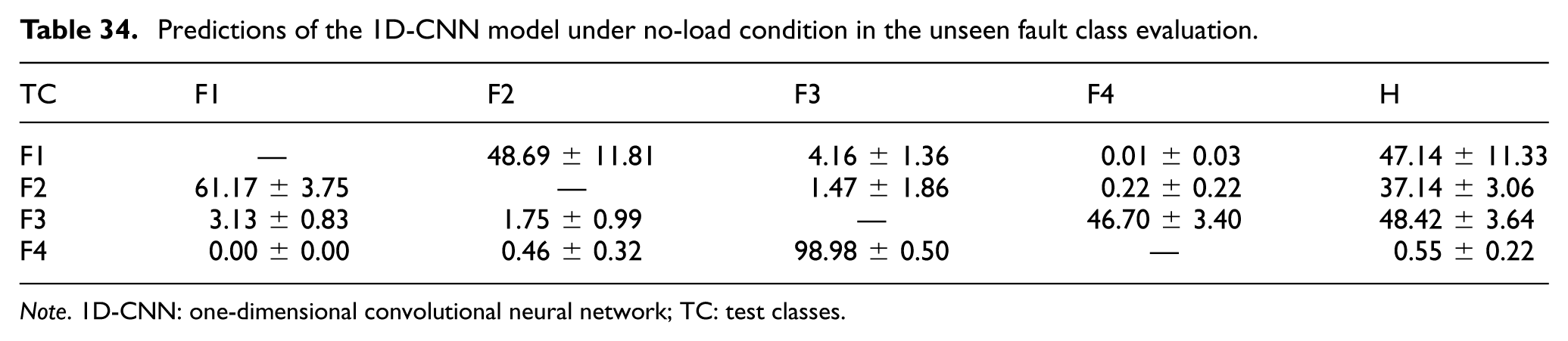
Tables 34 to 37 present the results obtained using the 1D-CNN method for the evaluation of generalization to unseen fault classes, organized by increasing load conditions. For each sub-experiment, one fault type was excluded from the training set, and then the classifier was trained with the remaining fault types. Subsequently, the classifier was tested with the excluded fault type to observe how the unseen samples were assigned to the known classes, including “Healthy.”
Predictions of the 1D-CNN model under no-load condition in the unseen fault class evaluation.
Note. 1D-CNN: one-dimensional convolutional neural network; TC: test classes.
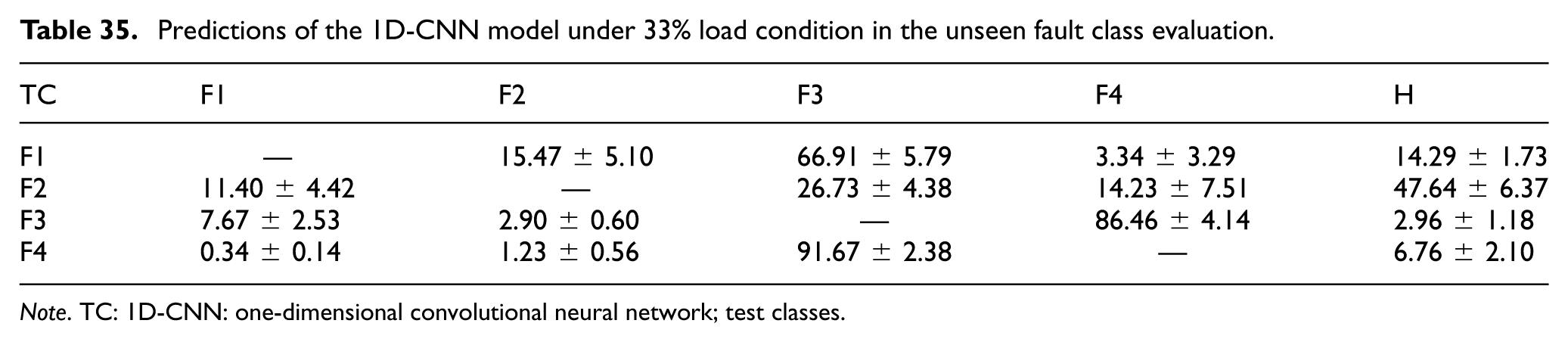
Predictions of the 1D-CNN model under 33% load condition in the unseen fault class evaluation.
Note. TC: 1D-CNN: one-dimensional convolutional neural network; test classes.
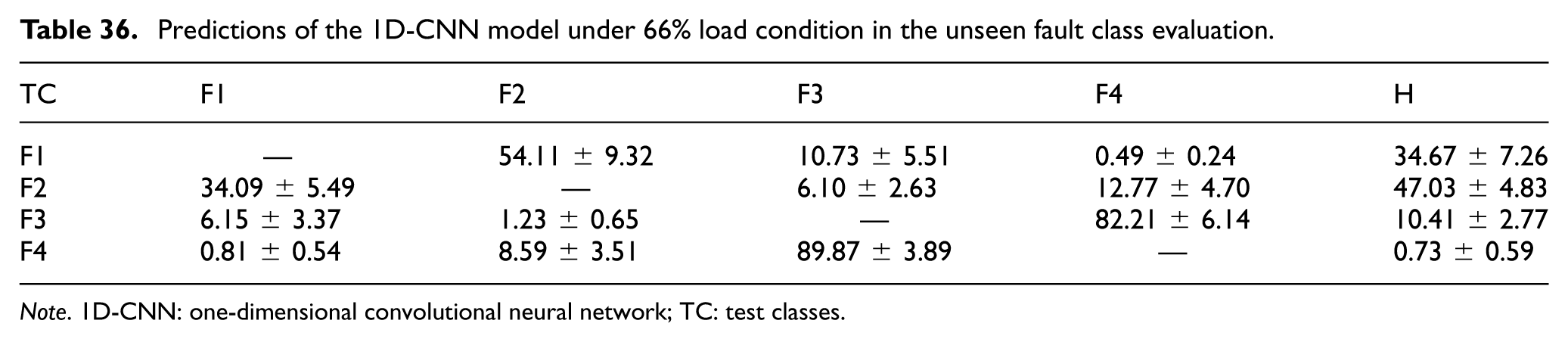
Predictions of the 1D-CNN model under 66% load condition in the unseen fault class evaluation.
Note. 1D-CNN: one-dimensional convolutional neural network; TC: test classes.
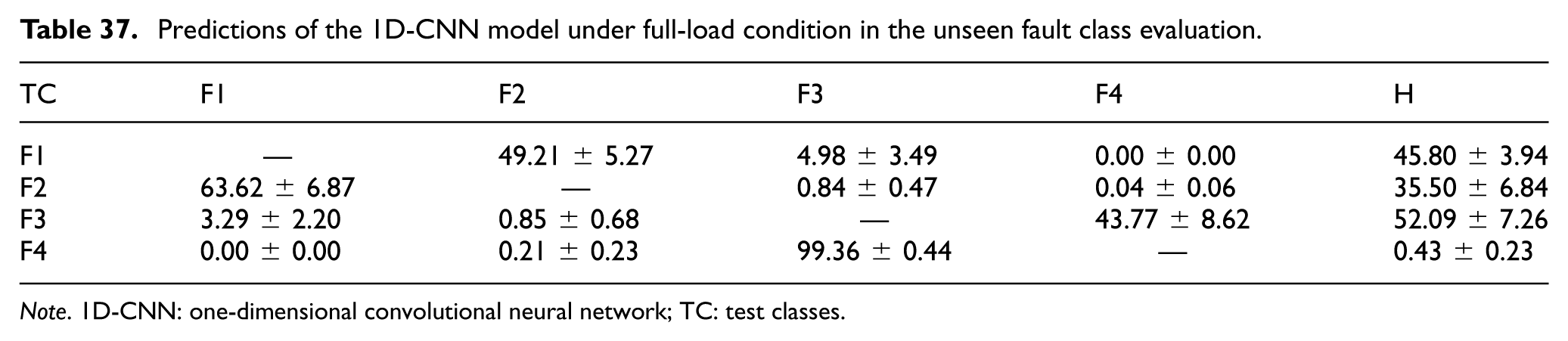
Predictions of the 1D-CNN model under full-load condition in the unseen fault class evaluation.
Note. 1D-CNN: one-dimensional convolutional neural network; TC: test classes.
Under the no-load (0%) condition (Table 34), the classifier showed substantial uncertainty when an unseen fault class was introduced. In particular, when Fault 1 was excluded from training, it was misclassified as “Healthy” at a rate of 47.14 ± 11.33%. A similar pattern was observed for unseen Fault 3, which was mapped to “Healthy” at a rate of 48.42 ± 3.64%. In contrast, unseen Fault 4 was assigned predominantly to Fault 3 (98.98 ± 0.50%), while the false “Healthy” rate remained low (0.55 ± 0.22%).
At the 33% and 66% load conditions (Tables 35 and 36), the assignment pattern of the unseen classes changed with the load level. For example, at 33% load, unseen Fault 2 was classified as “Healthy” at a rate of 47.64 ± 6.37%, whereas unseen Fault 3 was mapped mainly to Fault 4 (86.46 ± 4.14%).
In particular, under full-load conditions, the model again showed a tendency to place unseen intermediate faults near the “Healthy” boundary. At the 100% load condition (Table 37), unseen Fault 3 was classified as “Healthy” 52.09 ± 7.26% of the time. By contrast, unseen Fault 4 continued to be mapped almost entirely to Fault 3 (99.36 ± 0.44%), rather than to “Healthy.”
Overall, the 1D-CNN was able to group severe unseen faults into nearby faulty categories, but its tendency to assign early-stage or intermediate unseen faults to “Healthy” remains a clear limitation for fail-safe industrial deployment.
Generalization analysis of the 2D-AE model
The generalization behavior of the 2D-AE model, which uses 26× 26 data matrices, is summarized across different load conditions in Tables 38 to 41. Similar to the 1D-CNN, the 2D-AE maps unseen samples into the decision regions formed by the known classes. Under the 0% and 100% load conditions, the model showed broadly similar assignment patterns. Severe unseen faults were generally mapped to nearby faulty classes rather than to “Healthy.” For example, at 100% load, an unseen Fault 4 was assigned predominantly to Fault 3 (99.60 ± 0.74%). In addition, neighboring early-stage faults tended to map to one another, as reflected by unseen Fault 2 being classified as Fault 1 at a rate of 83.78 ± 6.23%. However, false “Healthy” predictions remained an important limitation. Most notably, unseen Fault 3 was classified as “Healthy” at rates of 45.62 ± 1.77% at 0% load and 45.30 ± 2.11% at 100% load.
Predictions of the 2D-AE model under no-load condition in the unseen fault class evaluation.
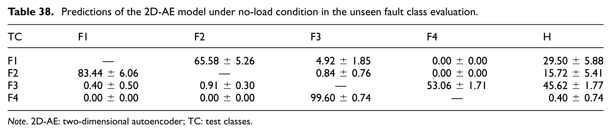
Note. 2D-AE: two-dimensional autoencoder; TC: test classes.
Predictions of the 2D-AE model under 33% load condition in the unseen fault class evaluation.

Note. 2D-AE: two-dimensional autoencoder; TC: test classes.
Predictions of the 2D-AE model under 66% load condition in the unseen fault class evaluation.
Note. 2D-AE: two-dimensional autoencoder; TC: test classes.
Predictions of the 2D-AE model under full-load condition in the unseen fault class evaluation.

Note. 2D-AE: two-dimensional autoencoder; TC: test classes.
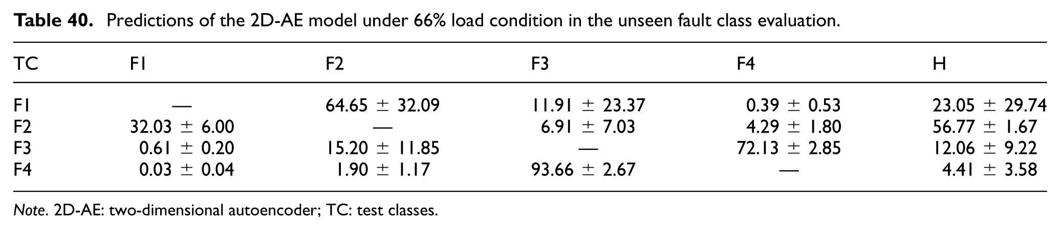
The model showed less stable behavior under transitional load conditions. At 33% load (Table 39), unseen Fault 1 was classified as “Healthy”49.41 ± 21.46% of the time, together with relatively large variation across runs. At 66% load (Table 40), unseen Fault 2 was mapped predominantly to “Healthy” (56.77 ± 1.67%). These results indicate that, although the 2D-AE performed well in the closed-set experiments, its deterministic latent representation was less effective at keeping unseen fault samples separated from the “Healthy” region, particularly under intermediate load conditions.
Generalization analysis of the 2D-VAE model
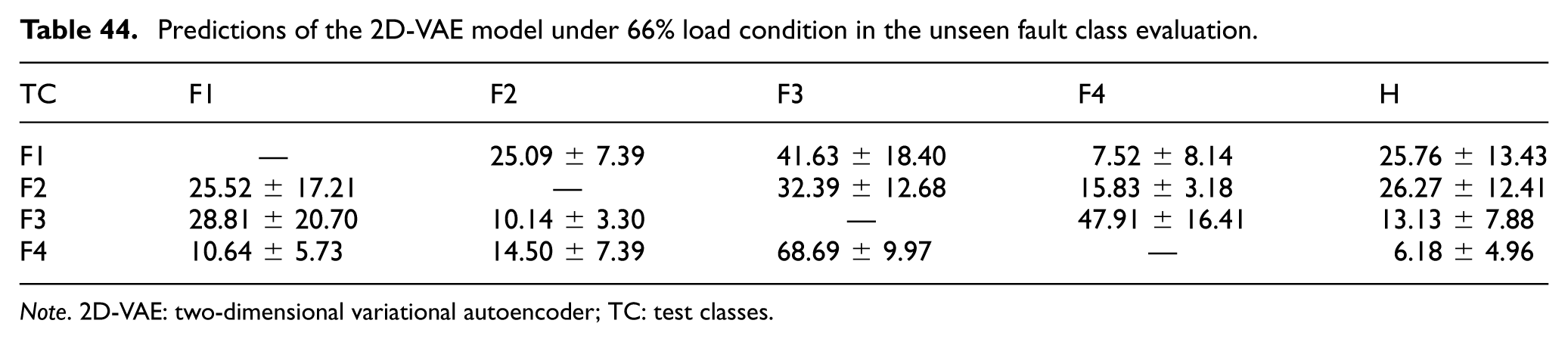
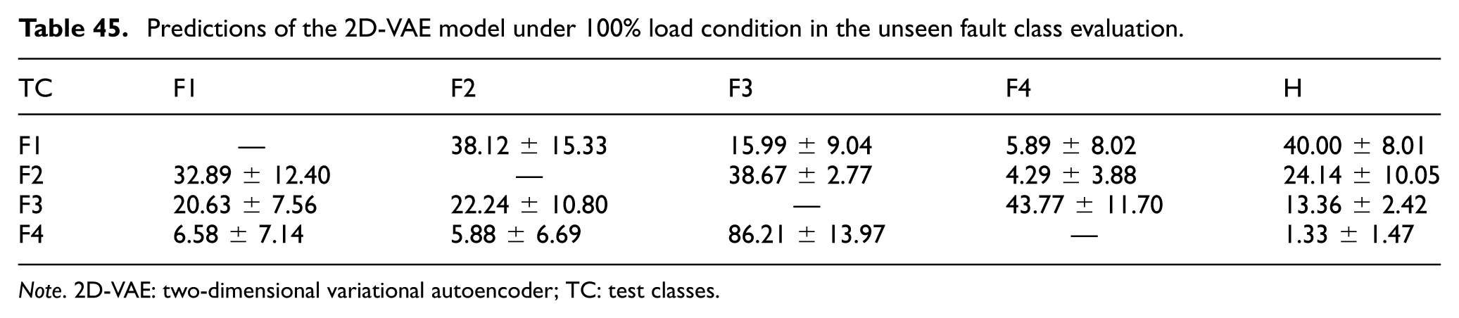
Tables 42 to 45 display the results from the 2D-VAE model under the evaluation of generalization to unseen fault classes, arranged by increasing load conditions. Similarly to the other models, one type of fault was excluded from the training set at each stage, and the classifier was trained on the remaining types of faults. The excluded fault type then served as the test set to evaluate how unseen samples were mapped to the known classes. The 2D-VAE differs from the deterministic models; in that, it learns a probabilistic latent representation, which leads to a more distributed assignment pattern for unseen samples.
Predictions of the 2D-VAE model under no-load condition in the unseen fault class evaluation.
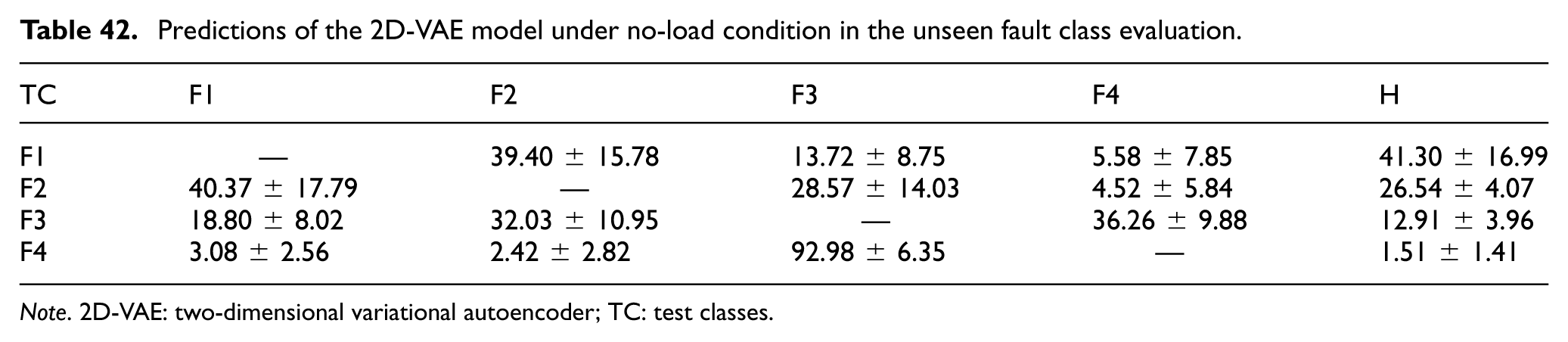
Note. 2D-VAE: two-dimensional variational autoencoder; TC: test classes.
Predictions of the 2D-VAE model under 33% load condition in the unseen fault class evaluation.

Note. 2D-VAE: two-dimensional variational autoencoder; TC: test classes.
Predictions of the 2D-VAE model under 66% load condition in the unseen fault class evaluation.
Note. 2D-VAE: two-dimensional variational autoencoder; TC: test classes.
Predictions of the 2D-VAE model under 100% load condition in the unseen fault class evaluation.
Note. 2D-VAE: two-dimensional variational autoencoder; TC: test classes.
Under the no-load (0%) condition (Table 42), Fault 1 did not collapse into a single known class; instead, it was mainly assigned to Fault 2 (39.40 ± 15.78%) and “Healthy” (41.30 ± 16.99%). Although the false “Healthy” rate remained non-negligible, the predictions were more distributed than those of the deterministic models. In contrast, when Fault 4 was excluded from training, the model avoided the “Healthy” boundary and mapped it predominantly to Fault 3 (92.98 ± 6.35%), with a false Healthy rate of only 1.51 ± 1.41%.
At the 33% and 66% load conditions (Tables 43 and 44), the 2D-VAE continued to suppress false “Healthy” assignments more effectively than the deterministic models. For example, at 33% load, unseen Fault 1 was classified as “Healthy” only 16.23 ± 9.96% of the time and was instead mapped mainly to Fault 3 (53.87 ± 22.42%). This suggests that the probabilistic latent representation tends to keep unseen fault patterns within the broader damaged region rather than allowing them to cross into the “Healthy” class.
Under full-load conditions, the overall behavior remained similar to that observed at no load. At the 100% load condition (Table 45), unseen Fault 1 was classified as “Healthy” at a rate of 40.00 ± 8.01%, whereas unseen Fault 4 remained well separated from the “Healthy” class, with a false “Healthy” rate of only 1.33 ± 1.47%.
Overall, although false “Healthy” predictions were not completely eliminated for unseen early-stage faults, the 2D-VAE showed the most stable behavior among the evaluated models. In particular, severe unseen faults remained within the damaged decision region rather than being misclassified as normal, which is a more desirable outcome for fail-safe industrial diagnosis.
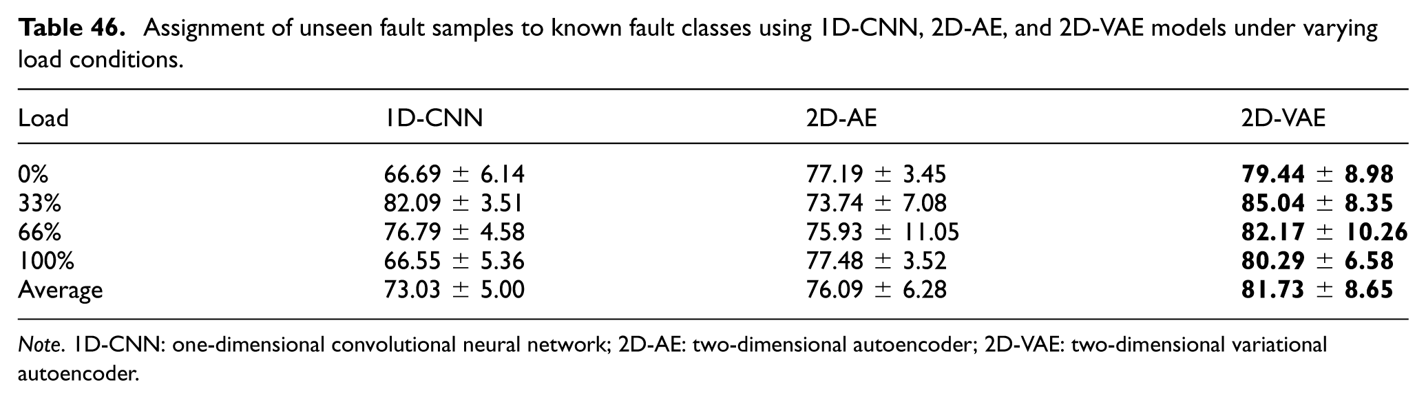
Table 46 presents a comparison of the rates at which the 1D-CNN, 2D-AE, and 2D-VAE models assign unseen fault samples to known fault classes, instead of the healthy class, across varying load conditions. The 2D-VAE method consistently outperforms both the 1D-CNN and 2D-AE models in all load conditions. While the deterministic models show larger performance variations across load levels—for example, the 1D-CNN reaches 66.69% under no-load conditions and the 2D-AE drops to 73.74% at 33% load—the 2D-VAE maintains comparatively stable performance, remaining around or above 80% in all test conditions. On average, the 2D-VAE achieves an overall success rate of 81.73 ± 8.65%, compared with 76.09 ± 6.28% for the 2D-AE and 73.03 ± 5.00% for the 1D-CNN. This pattern suggests that the probabilistic latent representation learned by the 2D-VAE may help the model keep unseen fault samples within damaged decision regions more consistently than the deterministic alternatives. Consequently, although none of the evaluated models completely eliminated false “Healthy” predictions for unseen faults, the 2D-VAE showed the most reliable overall behavior in this forced-classification setting. These results indicate that the 2D-VAE is the most reliable among the evaluated methods for applications in which previously unseen fault conditions may be encountered.
Assignment of unseen fault samples to known fault classes using 1D-CNN, 2D-AE, and 2D-VAE models under varying load conditions.
Note. 1D-CNN: one-dimensional convolutional neural network; 2D-AE: two-dimensional autoencoder; 2D-VAE: two-dimensional variational autoencoder.
Computational analysis and deployment considerations
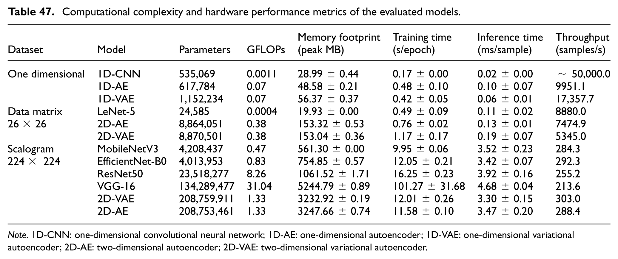
To examine the practical deployment characteristics of the evaluated methods for continuous condition monitoring, a computational analysis was performed. Table 47 summarizes the model complexity, memory requirements, and timing metrics of all evaluated methods. All benchmarks were conducted on a workstation equipped with an NVIDIA GeForce RTX 5070 12GB GPU, an Intel Core i7-14700F CPU, and 32 GB of RAM, using the PyTorch framework 80 with CUDA 12.8 acceleration.
Computational complexity and hardware performance metrics of the evaluated models.
Note. 1D-CNN: one-dimensional convolutional neural network; 1D-AE: one-dimensional autoencoder; 1D-VAE: one-dimensional variational autoencoder; 2D-AE: two-dimensional autoencoder; 2D-VAE: two-dimensional variational autoencoder.
Real-time implementation and edge deployment feasibility
Condition monitoring for industrial gearboxes benefits from timely processing of vibration data to support early fault detection and reduce the risk of severe mechanical damage. 81 The computational analysis highlights clear differences in deployment feasibility across the evaluated models. Deep 2D architectures such as VGG-16 and the scalogram-based 2D-VAE model exhibit relatively large memory requirements and higher parameter counts, which may limit their suitability for resource-constrained edge platforms.
By contrast, lightweight models such as the 1D-CNN offer very fast inference, although their generalization behavior under unseen operating conditions was less consistent than that of the best-performing latent-space models.
Among the evaluated methods, the 2D-VAE model utilizing 26× 26 data matrices provides a favorable balance between diagnostic performance and computational cost. With an inference time of approximately 0.19 ms per instance, the model can process about
Model compression and batch processing strategies
Although the proposed 26 × 26 data matrix-based 2D-VAE architecture is already more compact than the larger 2D models, additional optimization strategies may further improve its suitability for edge deployment. In particular, post-training quantization can reduce memory usage and inference cost, making the model easier to deploy on devices with tighter power, memory, or thermal constraints. Similar gains may also be achieved through pruning or deployment-oriented runtime optimization, depending on the target hardware.
For streaming vibration data, batch processing is not always necessary during standard online operation, where low-latency single-window inference is often preferred. However, small-batch execution may still be beneficial when multiple channels or parallel sensing nodes are processed simultaneously. In addition, overlapping sliding-window analysis can be used to support continuous monitoring while preserving temporal sensitivity to fault-related transients. In this setting, a buffer-based implementation can help maintain stable throughput and reduce the risk of data loss during periods of increased acquisition rate.
Overall, these considerations suggest that the 2D-VAE model is a practical candidate for real-time condition monitoring on edge-oriented industrial platforms, while also allowing further optimization through hardware-aware compression and deployment strategies.
Generalization considerations and limitations
Although the proposed VAE–SVM pipeline achieved strong diagnostic performance in the present experiments, its broader industrial generalization should be interpreted within the scope of the present validation setting. The current validation was conducted on a specific two-stage helical gearbox operating at a constant speed of 2678 rpm. Because vibration responses are influenced by machine configuration, gear and bearing characteristics, operating speed, load, and structural dynamics, the reported performance may vary when the method is transferred to different systems or to variable-speed operating conditions. In this respect, the representation-learning component may transfer more readily than the decision boundaries learned for the present gearbox, which are expected to remain more system-dependent.
In such cross-system scenarios, relying solely on a fully supervised classifier may be difficult, since newly deployed machinery rarely has sufficiently labeled fault data covering all relevant operating states. In our preliminary study, 37 we established an unsupervised anomaly-detection baseline using VAE reconstruction-error thresholds learned from healthy data only. That earlier setting was designed to separate healthy and faulty behavior at a binary level. In contrast, the objective of the present study is more demanding, as it targets multi-class classification of fault severity levels.
For practical deployment in previously unseen systems, a staged strategy may therefore be more suitable. For a new system with no available fault labels, an unsupervised or weakly supervised approach can be adopted initially using healthy baseline data. In this setting, VAE-based features may be combined with methods such as one-class SVM82,83 to support early detection of abnormal operating behavior. As labeled fault data become available over time, the diagnostic pipeline can then be extended toward the proposed multi-class framework.
To improve transferability across different speeds, gearbox configurations, or operating environments, future implementations may benefit from domain adaptation or transfer-learning strategies. For example, the VAE trained on the source system may be reused as an initialization and then adapted on a limited amount of target-domain data, while the downstream classifier is re-trained or fine-tuned for the new operating conditions. Before full deployment, validation on the target system should ideally include healthy baseline acquisition, evaluation under representative load and speed ranges, and limited fault-state verification whenever such data can be obtained.
Conclusion
This study investigated the detection and severity classification of distributed pitting faults in a two-stage industrial helical gearbox using vibration-based deep learning models under multiple load conditions. Distributed pitting produces more complex and overlapping vibration patterns, making it more difficult to diagnose than more localized fault signatures. To address this challenge, acquired vibration signals were evaluated in three input forms: 1D time-domain signals, 224 × 224 scalogram images, and 26 × 26 data-matrix representations.
The experimental results showed that model performance depended not only on the learning architecture but also on the suitability of the input representation. Among the evaluated approaches, the VAE-based model using the 26 × 26 data-matrix representation provided the most consistent overall performance across load conditions, while also offering a favorable balance between diagnostic accuracy and computational efficiency. Additional analyses under incomplete fault coverage further indicated that the learned representations could retain useful discriminative structure even when one fault class was excluded during training.
In general, the main contribution of this work lies in the systematic comparison of multiple diagnostic strategies for distributed pitting severity classification, with VAE-based representations emerging as the most consistent performers. At the same time, the transferability of these findings should be interpreted within the scope of the present validation setting, which involved a single gearbox configuration, artificially induced faults, and a constant operating speed. Future work may extend the present framework to broader operating conditions, different gearbox systems, and additional fault types to further assess its robustness and transferability.
Footnotes
Funding
The authors received no financial support for the research, authorship, and/or publication of this article.
Declaration of conflicting interests
The authors declared no potential conflicts of interest with respect to the research, authorship, and/or publication of this article.