
Abstract
Accurate remaining useful life (RUL) prediction of harmonic drives is essential for ensuring the safety of space manipulators. However, existing data-driven methods tend to use discrete time steps to predict RUL. These approaches ignore the actual physical degradation law of continuous degradation for mechanical equipment. To address this issue, taking neural ordinary differential equations as the core framework, this article proposes a state-adaptive liquid neural network (SALNN), which utilizes its unique liquid time-constant mechanism to characterize the RUL trajectory continuously. Specifically, prior to the prediction stage, a novel health indicator (HI) based on a spectral correlation architecture is constructed, targeting the fault characteristics of harmonic drives. Subsequently, SALNN utilizes a state detection module to perceive device degradation severity from the HI, embedding this as state information into the liquid time-constant, which can endow the network with dynamic properties. This mechanism enables the network to apply differentiated update rates corresponding to distinct degradation states, thereby capturing the physical evolutionary dynamics of the RUL more effectively. Experimental results on harmonic drive datasets and XJTU-SY dataset demonstrate that the proposed method effectively suppresses noise and significantly outperforms other state-of-the-art methods in prediction accuracy.
Keywords
Introduction
Advanced mechanical equipment is widely utilized in automobiles, aerospace, energy and power, and other fields. However, in industrial settings, prolonged operation, changing operating conditions, or improper maintenance can cause equipment to suffer damage. 1 Minor damage may lead to shutdowns and production losses, while severe damage may cause major safety accidents resulting in casualties. 2 Therefore, accurately estimating remaining useful life (RUL) and planning equipment maintenance in advance have become essential prerequisites for reducing the risk of accidents and ensuring stable equipment operation. 3
Under the framework of prognostic health management (PHM), RUL prediction methods for mechanical equipment are sorted into model-based and data-driven approaches. 4 Model-based methods primarily use mathematical knowledge or physical principles to construct models of equipment operation, thereby describing performance degradation. In research on bearing prognostics, many classical models have been proven by previous scholars to be instructive, such as the crack growth model, 5 the Archard wear model, 6 and Paris’ law model. 7 If the failure mechanism can be thoroughly analysed and the relevant parameters obtained, the model can accurately describe the degradation process, enabling RUL prediction. However, this approach has several limitations. The internal damage mechanisms of complex mechanical systems are difficult to analyse, making it challenging to construct appropriate physical models. 8 Furthermore, model parameters are usually determined from extensive experimental data or finite element simulations, resulting in high acquisition costs. 9 Consequently, in scenarios characterized by massive data volumes and complex operating conditions, model-based methods face difficulties in further development, while data-driven approaches are gradually becoming mainstream for RUL prediction. 10
In general, data-driven methods for mechanical equipment prognostics can be implemented in four steps: data collection and processing, constructing HI, segmenting health stages, and predicting RUL. HI construction and RUL prediction are crucial steps in the method. HI construction serves as a link connecting raw monitoring data to the health status of equipment, while RUL prediction is the ultimate goal of machinery health prognostics. 11 Recent review studies have provided a systematic summary of RUL prediction methodologies with HI dependence for rotating machinery, highlighting the central role of HI construction and its relationship to subsequent prognostic modelling. 12 This article focuses on improving data-driven methods, particularly in HI construction and network model design.
Constructing an HI that accurately characterizes the trend of equipment degradation is a prerequisite for estimating RUL, since the RUL prediction problem is essentially a regression task that models equipment degradation using the HI. 13 Based on the construction method, HIs are categorized into physical health indicators (PHIs) and virtual health indicators (VHIs). PHIs are proposed based on the physical mechanisms of the degradation process. Common PHIs include the root mean square (RMS), the kurtosis, and the indicator of second-order cyclostationarity (ICS2), which describe the state of bearings from the perspectives of energy, impact characteristics, and cyclostationarity, respectively. Entropy-based indicators, such as sample entropy and fuzzy entropy, assess the degree of system disorder based on signal complexity. RMS is the most commonly used HI for assessing bearing performance and is the indicator that effectively reflects signal energy. The RMS 14 was used as a time-domain feature to capture the bearing degradation trend in research work. Pan et al. 15 proposed using a relative RMS value, optimized via linear rectification, as the HI for RUL prediction. In addition, mechanical equipment fault signals can manifest as periodic impulses. Thus, impulsiveness and cyclostationarity are regarded as two key attributes for characterizing degradation behaviours. 16 Kurtosis and second-order cyclostationarity are typical indicators of these properties. For instance, in study, 17 kurtosis was employed as an input feature for a Support Vector Regression network to compare prediction performance. Dong and Chen 18 , as well as Feng et al. 19 utilized the second-order cyclostationarity of vibration signals to construct an HI characterizing degradation trends of bearings and gears. Entropy characterizes equipment degradation by quantifying the system’s disorder. However, VHIs utilize virtual representations to reveal the bearing degradation process. In the study, 20 a matrix factorization method was used to iteratively solve a slow-feature HI. Bai et al. 21 proposed using genetic programming to adaptively fuse features for constructing HI.
In actual operating environment, monitoring data is often subject to external noise interference, which causes random fluctuations in HI curves and impairs their ability to characterize degradation trends. To reduce the impact of noise and random fluctuations, relevant studies have proposed the following methods: Under the spectral correlation framework, Ni et al. 22 introduced Linear Rectification-Wasserstein Distance Spectral Correlation (LR-WDSC), combining the Wasserstein distance and optimized via linear rectification to achieve high-precision bearing RUL prediction. In another study, Ni et al. 23 constructed a WDgram multi-scale feature map and used a multi-objective grasshopper optimization algorithm to generate the Composite Multi-scale Wasserstein Distance (CMSWD). Kuzio et al. 24 conducted local damage detection of bearing vibration in the presence of non-Gaussian noise, then constructed a HI by comparing the distance between the information and non-information bands in cyclic spectrum coherence diagram. Xu et al. 25 introduced a bearing HI derived from the moving average cross-correlation coefficient of power spectral density. Cohen et al. 26 developed a multi-slice dynamic model for helical gears with tooth breakage. They also proposed a novel spectral-energy HI, refuting the assumption that fault severity correlates with damage size. Inspired by these studies, this article proposes a novel PHI that reflects the energy of vibration signals.
In data-driven equipment prognostics, the selection of neural networks also plays a vital role in prediction accuracy, generalization ability, and engineering applicability of RUL prediction. Commonly used neural networks include gated recurrent unit (GRU), long short-term memory (LSTM), graph neural networks (GNNs), and Transformers. In terms of feature extraction, GRUs and LSTMs are biased toward extracting temporal features. Li et al. 27 combined Convolutional Neural Network (CNN) feature fusion with GRU to propose an Integrated Deep Multi-scale Feature Fusion Network, which utilizes the Mish activation function to achieve high-precision lifetime prediction on the C-MAPSS dataset. Wang et al. 28 proposed a Gated Graph Convolutional Network that integrates multi-sensor fusion for RUL prediction. Xu et al. 29 proposed a multi-resolution LSTM for aero-engine RUL prediction and addressed the complex operating conditions of aero-engines. Shi et al. 30 proposed a lightweight model based on exponential smoothing and an attention-enhanced LSTM, addressing the issues of attention mechanisms losing temporal information and the complex model deployment. In contrast, GNNs and Transformers are suited to extracting spatial features. Wang et al. 31 constructed a spatio-temporal graph via dynamic time warping and proposed a Graph Feature-based Graph Convolutional Attention Network to address the challenge of predicting aero-engine lifespan with partially missing multi-sensor data. Cai et al. 32 introduced a Knowledge-Embedded Spatio-Temporal Graph Convolutional Network that utilizes prior knowledge to model sensor spatial interactions. Xu et al. 33 developed a spatiotemporal hybrid Transformer variant to address RUL prediction challenges involving multiple operating conditions and high-dimensional multi-sensor features.
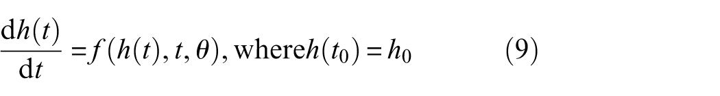
Current data-driven methods for equipment RUL prediction primarily improve prediction accuracy by modifying network architectures or optimizing optimization strategies, with research focusing on spatio-temporal representations, transfer learning and continual learning. Wang et al. 34 proposed a Dual-View Graph Transformer to address the challenges of feature fusion arising from complex spatiotemporal dependencies in RUL prediction. Wang et al. 35 combined multi-task learning, dual-level adversarial transfer learning, and multi-level attention to predict the RUL of CNC milling tools in parallel. Qian et al. 36 proposed a Dimension-Mismatched Adversarial Network for rolling bearing RUL transfer prediction under cross-domain scenarios with mismatched input dimensions. Zhou et al. 37 proposed a Knowledge Library Network for non-exemplar incremental RUL prediction to achieve accurate prediction across sequential tasks while alleviating catastrophic forgetting. However, such methods generally have limitations: their predictive processes are disconnected from physical degradation laws and fail to account for the underlying physical dynamics of equipment from health to failure. For example, the degradation process of equipment such as bearings and engines has inherent “irreversible and progressive” properties. Yet, existing methods mostly adopt a point-prediction paradigm, producing discrete outputs that often yield fluctuating prediction trajectories that violate physical laws. 38 Predicting RUL from a trajectory modelling perspective can effectively address this limitation. The equipment degradation process is essentially a continuous, smooth evolution of system states. Characterizing temporal dependencies by predicting state derivatives between time steps enables the establishment of RUL trajectories that conform to physical laws and have causal relationships. As abstract descriptions of dynamic systems, Neural Ordinary Differential Equations (NODEs) are suitable for such trajectory modelling. Its recursive property can simulate the degradation process where the current state depends on historical evolution, and can integrate physical priors through explicit dynamic equations. 39
As a result, NODEs have attracted significant attention for RUL prediction. On the one hand, these models can simulate continuous degradation trajectories using numerical solvers, avoiding the fluctuation issues inherent to point prediction. Zhou et al. 38 proposed a Dynamic Governing Network that employs a parameterized NODES as the governing equation for the RUL trajectory, thereby aligning the output trajectories closely with actual degradation by constraining the degradation rate. On the other hand, NODEs grant these models stronger generalization capabilities. Hu et al. 40 used the time-invariance property of NODEs to learn consistent features across different degradation stages, effectively mitigating distribution shifts in single-source domain generalization scenarios. Hasani et al. 41 introduced a liquid time-constants (LTCs) model that uses time-varying constants in NODEs to simulate dynamic changes in sensitivity during equipment degradation. This model has demonstrated superior stability and accuracy compared to LSTM and traditional NODEs in temporal modelling task. However, due to the LTCs network’s excessive sensitivity and the lack of interpretability in PHM, this article proposes a novel LTC network and applies it to RUL prediction.
The framework is shown in Figure 1, and the innovations and contributions of this article are reflected in the following aspects:
(1) The Targeted Cyclic Energy Indicator (TCEI) is constructed based on second-order cyclostationary properties. Through spectral correlation analysis, it selectively extracts energy at specific cyclic frequencies and fault-related frequency bands. By combining the mean fault-symptomatic peaks (MFP) with screening high-energy fault bands, it suppresses noise interference and prevents misjudgment of irrelevant frequency bands. Additionally, exponential smoothing is applied to reduce random fluctuations.
(2) This article proposes state-adaptive liquid neural network (SALNN). To address the dynamic differences between the healthy and degraded stages of mechanical equipment, a dual-time-constant system is designed. Guided by the health probability output from a state discriminator, it adaptively controls the initial values and fluctuation ranges of the time constants. This allows the model to capture long-term trends during healthy states and respond to short-term fluctuations in the degradation stage, resolving the oversensitivity and fluctuation issues of traditional LTC networks.
(3) Extensive experiments are conducted on the harmonic drives and the bearings. The results validate the performance advantages of the proposed indicator and model.
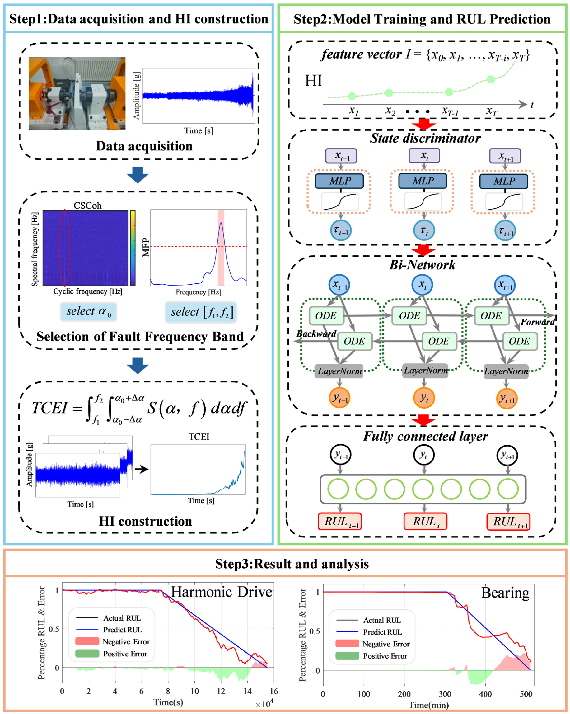
Framework of the proposed method.
The main structure of the present article are as follows: section “Construction of the novel HI” presents the detailed methodology for constructing HI from a signal processing perspective. Section “The proposed prognostic approach” elaborates on the technical details of the proposed prediction methodology. Section “Case 1: Harmonic drive dataset” and section “Case 2: XJTU-SY dataset” present the experimental validation and performance evaluation of the proposed method on two distinct datasets, respectively. Section “Conclusion” provides a systematic summary and conclusion of the overall research work presented in this article.
Construction of the novel HI
This section conducts a deep study of second-order cyclostationary indicators, targeting the fault characteristic frequency bands of vibration signals to construct an energy indicator that reflects potential degradation features of rotating machinery. The following describes the methodology for building a novel second-order cyclostationary energy indicator based on spectral correlation analysis and frequency band selection criteria.
Spectral correlation analysis
Vibration signals generated by rotating machinery faults, such as gear tooth surface wear and bearing pitting, are typically considered a chain of periodic impulses. However, when operating, the arrival intervals between two consecutive fault impacts exhibit random slips, which transform the signal from an ideal periodic signal into a periodically time-varying signal. This property has inspired extensive research into first- and second-order cyclostationary signals in industrial settings. The rotating machinery fault signals belong to the second-order cyclostationary signals, manifested as periodic fluctuations of their second-order autocorrelation functions in time 42 :
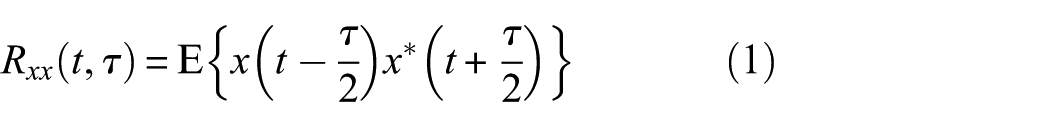

where
Since the spectral correlation function can characterize the information contained in second-order cyclostationary signals, spectral correlation has become one of the most widely used methods among various second-order cyclostationary analysis techniques. The spectral correlation function below can be obtained by performing Fourier transforms on the instantaneous autocorrelation function in both the time and time-lag dimensions:
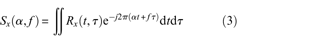
where
Fault information estimation
To screen for high-energy fault characteristic frequency bands in the spectral correlation map, this article proposes MFP to identify energy values. The original MFP to the noise (MFPN) uses “peak-to-noise ratio” to evaluate fault information in frequency bands. Although it can effectively suppress noise interference, it tends to misjudge high-energy bands as invalid under intense background noise or when overall resonance energy is high. In this engineering context, this article improves MFPN by removing the average noise term from the original denominator and retaining the numerator. Finally, for each cyclic frequency slice, the spectral correlation amplitudes are accumulated according to preset fault frequency orders, yielding a curve that reflects the accumulation of fault energy. The larger the amplitude of the curve, the stronger the resonance energy caused by fault impacts in the corresponding frequency band. High-energy fault frequency bands can thus be obtained without additional penalty terms. The formula for the fault feature peak indicator is as follows 43 :
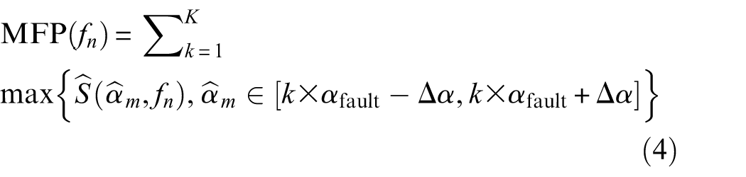
where
Construction of TCEI
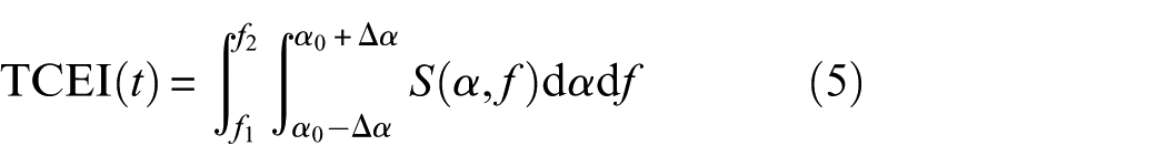
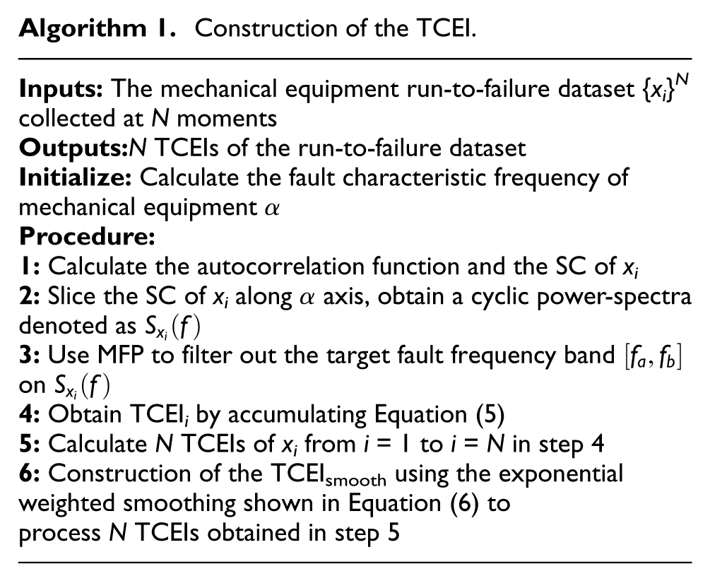
To construct the novel HI, the acquired vibration signals are subjected to spectral correlation analysis. The corresponding fault characteristic frequencies are calculated according to the formulas. Subsequently, the MFP indicator is employed to screen the target frequency bands. Finally, the fault characteristic frequencies, the screened fault frequency bands, and the spectral correlation map are incorporated into the energy integration formula to calculate the TCEI for that specific time step. By computing this sequentially for each time step, the full-life cycle TCEI indicator is obtained.
where
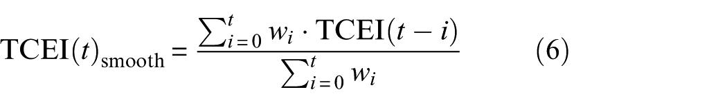
From the perspective of predicting degradation trajectories, the stochastic fluctuations within the HI fail to convey meaningful information about bearing degradation. Instead, the model can make them unnecessarily complicated during training, leading to additional parameters that fit the noise. This ultimately compromises prediction accuracy and robustness. Therefore, the exponential smoothing technique is employed to mitigate fluctuations during mechanical equipment degradation, facilitating better extraction of the underlying degradation trend characteristics. Algorithm 1 outlines the entire process, while the construction and smoothing formula for TCEI is as follows 30 :

where the decay factor
Construction of the TCEI.
The proposed prognostic approach
This section introduces a deep learning model designed for RUL prediction. The model’s predictive workflow primarily consists of three components: state detection, feature extraction, and RUL prediction. The state discriminator first analyses the HI sequence using the model. The detection results directly determine the time constants, which, in turn, govern the update rates of subsequent hidden states. Subsequently, an improved NODEs network is employed to iteratively extract latent representations of the degradation features from hidden states. Finally, the iterative results are fed into a fully connected layer to arrive at the last forecast of RUL.
Neural ordinary differential equation
In previous studies, most researchers treated RUL prediction as a time-series modelling task and used traditional time-series models, such as GRUs and LSTMs. However, mechanical equipment degradation is a continuous, dynamically evolving process, while these time-series methods are discrete-time models that record historical information through jumps across multiple discrete time steps. They tend to suffer from gradient explosion in long sequences, and temporal correlations are unstable, making it challenging to capture the essence of degradation dynamics. In recent years, a new neural network framework based on ordinary differential equation (ODE) has been proposed. It defines the hidden state of a neural network as the solution to an ODE, modelling the system’s evolution process in time domain. This network architecture is not only more suitable for time-series modelling tasks but also highly consistent with the physical meaning of mechanical equipment degradation. The formula for parameterizing the continuous dynamics of hidden units using ODE is as follows 39 :
where
In light of this, several variants of NODEs have emerged in the field of artificial intelligence. Inspired by biological nervous systems, Hasani et al. 41 proposed the LTC network that combines a presynaptic neuron current architecture with a neuron membrane potential equation:

where
Hasani proposed the dynamics of LTCs represented by the following equation 41 :
where
To improve computational efficiency, Hasani developed a custom hybrid solver rather than using general solvers. This solver combines the advantages of both Explicit and Implicit Euler methods. The solver expression is as follows:
where
State-adaptive liquid neural network
This article introduces the LTC networks into RUL prediction, then proposes improvements on the significant difference in dynamic behaviour between healthy and degraded states, based on mechanical equipment degradation characteristics. A novel ODE network is designed that combines a dual-time-constant system and a state discriminator.
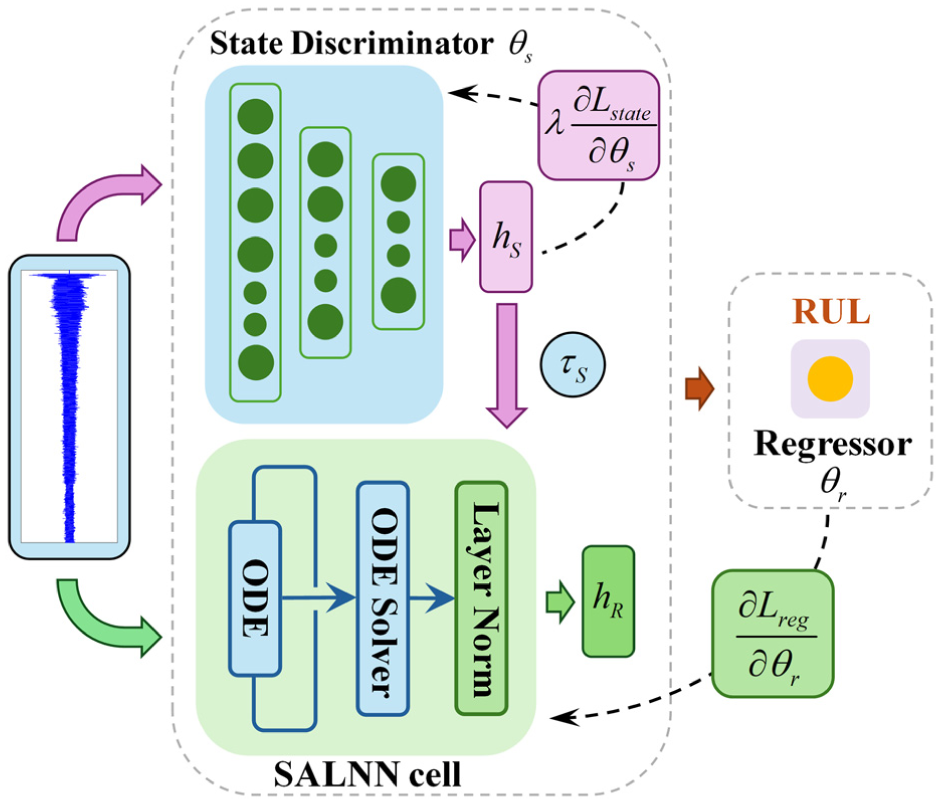
The network architecture and RUL prediction process are illustrated in Figure 1. The HI sequence is fed into both the state discriminator and the LTCs cell units simultaneously. The state discriminator analyses the sequence to output a health-state probability, which can then be used to regulate the time constants. The LTCs cell units utilize these time constants to establish ODEs. A hybrid-form solver performs numerical solution, and the output is passed through a LayerNorm layer to ensure stability during training. The entire network adopts a bidirectional extraction architecture. Finally, the output layer maps the ultimate hidden state to the predicted RUL. This network design balances physical interpretability with computational efficiency, preserving the advantages of trajectory modelling while enhancing the capability to capture degradation laws.
The dynamic behaviour of time constants directly determines the accuracy of ODE models in capturing degradation. To achieve precise state recognition, a deep neural network discriminator is constructed. This discriminator adopts a multi-layer perceptron architecture, enhances classification training stability through batch normalization layers, and outputs a continuous probability estimate of the equipment health state via a sigmoid activation function. The process of state classification is shown in Figure 2 and the following formula can represent the structure of the discriminator:


where
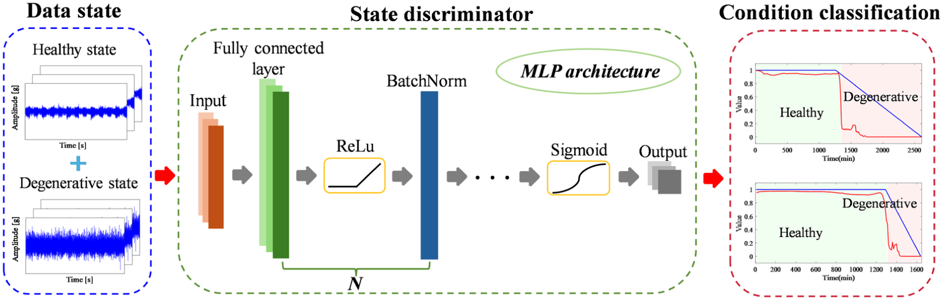
Flowchart of the state classification.
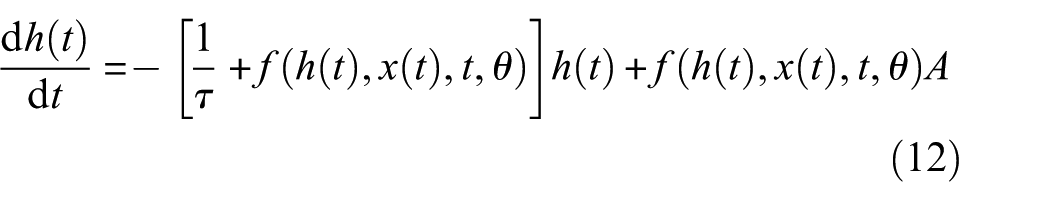
From a mechanical degradation perspective, the time-constant-related term can be viewed as a damping term that regulates the rate of equipment degradation. Based on the state-aware mechanism, this article further enhances the model’s adaptability to multi-stage degradation processes by designing a differentiated time-constant system for two typical stages. The two typical stages are healthy and degraded, with specific differences reflected in two aspects: initial value setting and fluctuation range. In the healthy stage, mechanical equipment operates stably with a slow degradation rate and gentle changes. Therefore, a larger initial value of the time constant and a narrower fluctuation range are selected. This setup can reduce model sensitivity to short-term minor noise, focus on capturing long-term, stable evolutionary trends of the healthy state, and avoid misjudging the equipment degradation process due to local fluctuations. In the degraded stage, mechanical equipment performance declines rapidly, and fluctuations in operating conditions intensify. Thus, a smaller initial value of the time constant and a wider fluctuation range are adopted. This configuration enhances the model’s responsiveness to short-term degradation features, accurately captures key dynamic information, such as sudden changes in equipment performance and aggravated faults, and ensures real-time tracking of the degradation process.
The state-adaptive time-constant differential equation is as follows:
where
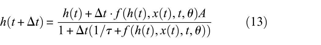
Although the hybrid solver adopted in this article is based on a core logic of implicit solvers, it ultimately yields a closed-form analytical solution. This characteristic eliminates the need for complex, time-consuming, iterative operations at each numerical computation step, placing its computational load in the same order of magnitude as that of the Explicit Euler method. From a numerical stability perspective, the implicit formulation inherently yields a superior solution to the differential equation. In contrast to explicit methods, which are prone to numerical oscillations due to step-size sensitivity, this hybrid solver allows SALNN to adopt larger computational step sizes during simulation. This effectively avoids system divergence caused by inappropriate step-size settings and reduces solution risk during model training and prediction. Considering the solver’s mathematical structure, the denominator term functions similarly to an adaptive stabilizer. When the equipment degradation system undergoes sharp dynamic changes, such as sudden shifts in degradation rate or abrupt increases in fault characteristics, the denominator term responds promptly by increasing. In turn, this reduces the magnitude of hidden-state updates, preventing abnormal feature extraction caused by severe system fluctuations. This structural design also enhances the robustness of the model computational process and ensures stability in modelling complex degradation processes.
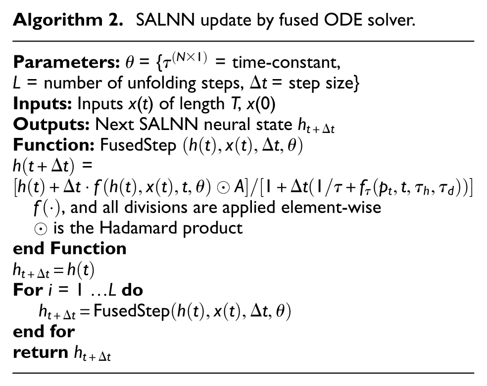
The selection of the differential solver references the hybrid solver proposed in the LTC network. Algorithm 2 is the ODE solver iterative solution. 41 The solution formula is as follows:
SALNN update by fused ODE solver.
RUL prediction and loss function
To ensure stable output from the RUL prediction layer, this article introduces normalization into model training: the hidden-state output from each iteration of the ODE is fed into a LayerNorm layer. Through standardization, gradient fluctuations during training are suppressed, and the instability of model training caused by deviations in the feature distribution is avoided.
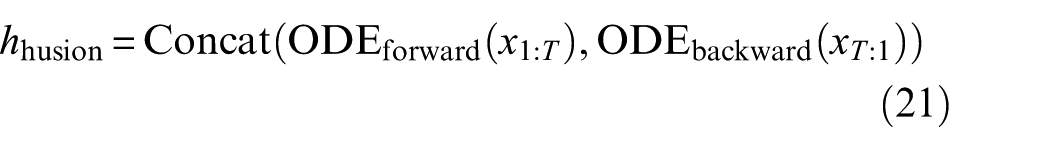
In addition, to fully explore the temporal correlation in equipment degradation and to prevent the omission of historical or future degradation information due to one-way feature extraction, this article embeds the entire ODE neural network framework within a bidirectional extraction architecture. This architecture consists of two parallel feature extraction branches, a forward branch and a backward branch. The forward branch iterates from the start to the end, capturing features during the “healthy-degraded” process; the backward branch iterates from the end to the start, mining degradation-traceability information implied by the “faulty-healthy” process, such as the retrospective capture of early weak fault features. The hidden states of the two bidirectional branches are finally fused through feature concatenation to form comprehensive degradation features that contain both forward and reverse temporal information. These features are then fed into a fully connected layer, which performs dimensionality reduction and a nonlinear mapping to produce an RUL prediction. The feature fusion process of the bidirectional architecture and the mathematical expression of RUL prediction are as follows:


where
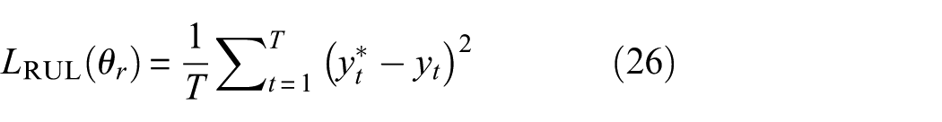
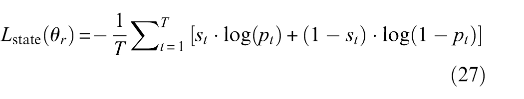
The SALNN proposed in the article is essentially a multi-task collaborative learning framework, which integrates two tasks: the RUL prediction task and the state monitoring task. Two tasks have a strong coupling relationship. The recognition accuracy of the state monitoring task directly determines adaptive regulation of the time constant, which in turn affects the model’s prediction accuracy. To address the problem that a single-task loss function is complex to optimize for simultaneously improving the discriminator performance, this article proposes a dual-supervised loss function. By jointly optimizing an objective, this loss function enables collaborative training. On the one hand, it minimizes the difference between the forecasted and actual RUL values; on the other hand, it improves the state discriminator ability to identify the critical transition point between the equipment’s healthy and degraded states. Ultimately, this ensures the effectiveness and stability of model training.
This dual supervised loss function is composed of a regression loss term and a classification loss term, each with a weight, corresponding to the optimization objectives of the RUL prediction task and the state monitoring task, respectively. The backpropagation construction is shown in Figure 3. Its mathematical expression is as follows:

where
The backpropagation of SALNN. SALNN: state-adaptive liquid neural network.
Case 1: Harmonic drive dataset
Dataset description
The full-life cycle test for harmonic drives was conducted on an aerospace power system comprehensive performance test platform. As shown in Figure 4, the test bench primarily comprises three components: a drive motor, a load motor, and harmonic drives test units. Vibration signals along the x, y, and z axes are simultaneously acquired using two accelerometers. Data collection occurs at 10-min intervals, with each sampling session lasting 5 s at a sampling frequency of 12.8 kHz.
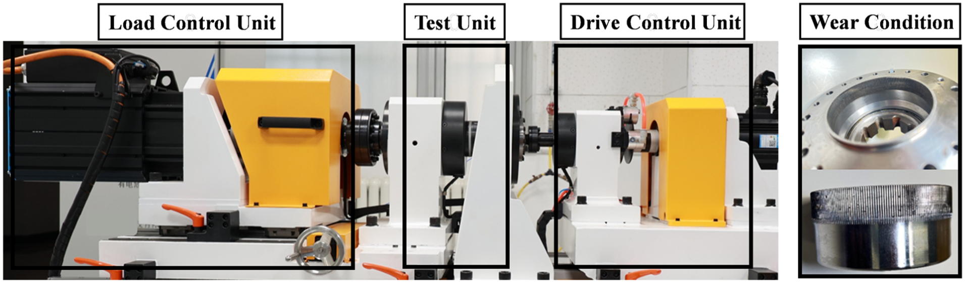
Photo of test bench and harmonic drive fault parts.
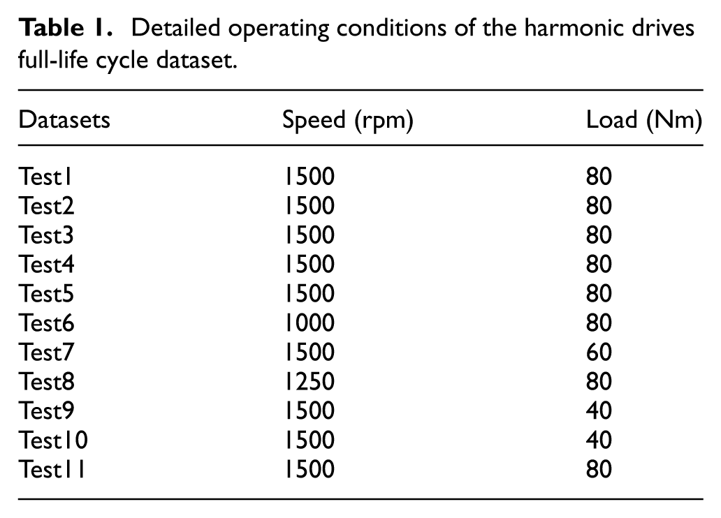
The experimental campaign includes 11 independent tests, generating 11 distinct data subsets that encompass multiple operational condition combinations. These comprise three rotational speed levels (1000, 1250, and 1500 rpm) and three load levels (40, 60, and 80 Nm). Detailed operational parameters for each subset are provided in Table 1. For model training and validation, leave-one-out cross-validation is used. During each iteration, one of the 11 subsets is chosen as the test set, and the other ten are utilized for training. The training set is divided into training and validation subsets in a 4:1 ratio to aid in optimizing model parameters and avoiding overfitting.
Detailed operating conditions of the harmonic drives full-life cycle dataset.
Selection of cycling frequency and fault frequency band
Before constructing the TCEI, it is essential to determine the key parameters required for its calculation: the cyclic frequency and the fault frequency band. The selection of these parameters directly dictates the indicator’s ability to characterize the equipment’s degradation trend. Insufficient parameter matching will result in an indicator that fails to reflect the equipment’s actual degradation state accurately.
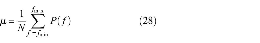
Using the full-life cycle dataset, Test3 as an analysis sample, a segment of its vibration signal is extracted for visual analysis, as shown in Figure 6(a). The time-domain waveform shows the signal is contaminated by noise, making it impossible to directly identify the fault characteristics of the harmonic drive. Therefore, the fault type is defined based on actual damage observed in the harmonic drive. The damage in Test3 primarily manifests as wear. The tooth surface of the test piece flexspline was observed under a microscope. The result is shown in Figure 5. Degradation phenomena such as wear on the flexspline, circular spline, and the contact surface between the wave generator and flexspline lead to a reduction in meshing stiffness and an increase in clearance between components. 44 This change has two main effects: first, an offset of the instantaneous centre, and second, a bi-periodic fluctuation in meshing stiffness. In the demodulated spectrum, this modulation phenomenon is evidenced by an increase in the amplitude at twice the rotational frequency and its harmonics. Correspondingly, the spectral correlation map also shows high energy concentration at twice the rotational frequency. Therefore, twice the rotational frequency is identified as the cyclic frequency for the harmonic drive.
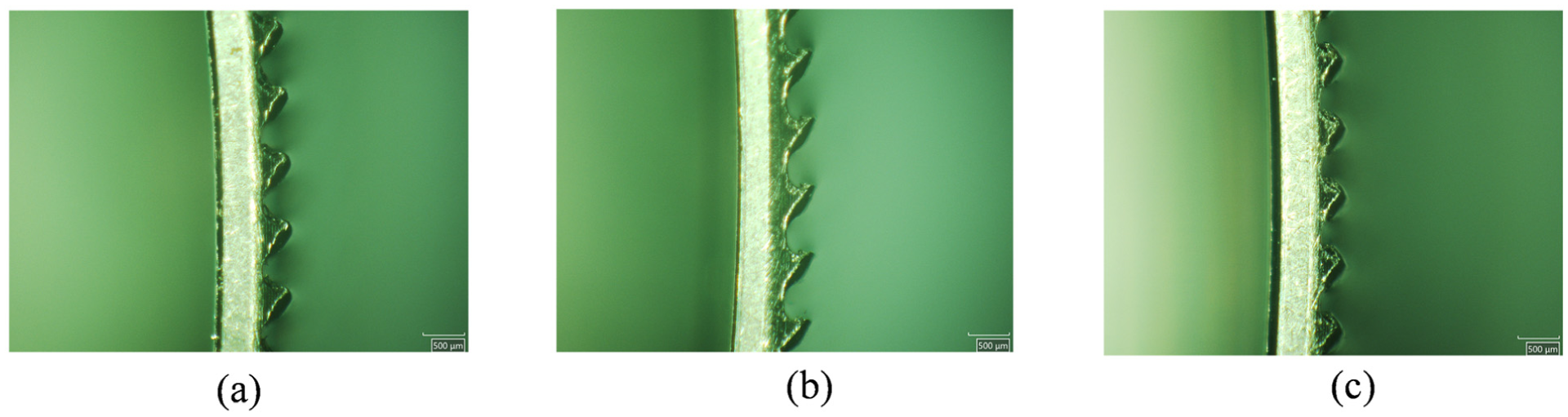
Tooth surface wear: (a) Test2, (b) Test3, and (c) Test7.
To further screen for sensitive fault frequency bands, the MFP is employed to analyse the energy distribution across frequency bands. The result is shown in Figure 6(c). The statistical characteristics of the MFP curve across the entire frequency range are calculated, using the mean plus two standard deviations as the high-energy threshold for screening. Continuous frequency points exceeding this threshold are then selected as the fault frequency band. The screening formula is as follows:

where
Test3 vibration analysis: (a) time domain signal, (b) spectral correlation, and (c) frequency band selection.
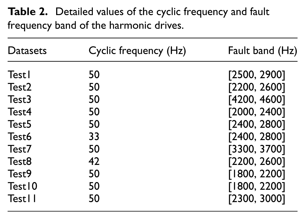
Consequently, the range [4200, 4600] Hz is chosen as the integration interval for the fault frequency band, which will be used for the subsequent energy calculation of the TCEI. Based on the above analysis, cyclic frequency and fault frequency band screening were conducted for all 11 groups of harmonic drive datasets. Finally, the fault frequency bands required for TCEI calculation for each dataset were determined, with appropriate rounding applied. The screening results of fault frequency bands for all equipment are shown in Table 2.
Detailed values of the cyclic frequency and fault frequency band of the harmonic drives.
TCEI
To capture the degradation trajectory of the harmonic drives and reflect its degradation characteristics, the optimal parameters screened were substituted into TCEI calculation formula for feature extraction from each acquired vibration signal segment. Taking datasets Test3 and Test4 as examples, the extracted TCEI curves are shown in Figure 7, respectively. As illustrated, the TCEI curves for both datasets exhibit clear multi-stage degradation characteristics. During the first half of the service cycle, TCEI values remain low, indicating stable and healthy equipment operation. In the latter half, TCEI values show a continuous upward trend, reflecting gradual performance deterioration that ultimately leads to failure. These results validate the effectiveness of TCEI in characterizing the degradation process of the harmonic drive.
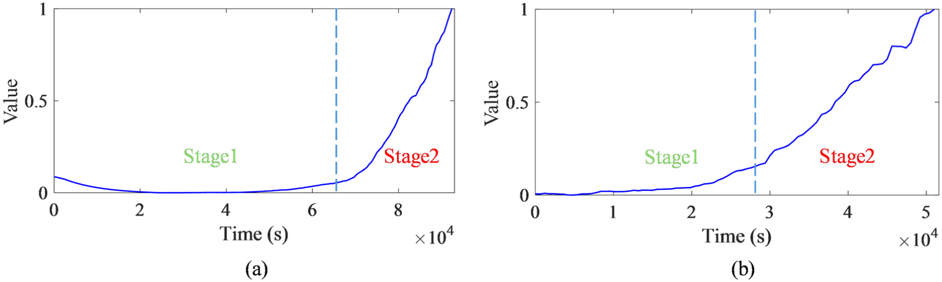
TCEIs: (a) Test3 and (b) Test4.
This article conducts a quantitative analysis from three dimensions, monotonicity, correlation, and robustness, and compares it with traditional HIs to evaluate the performance of TCEI systematically. 45 The definitions of each evaluation indicator are as follows 46 : Monotonicity measures the degree to which a mechanical equipment’s HI changes monotonically over time, reflecting the irreversibility of the degradation process. Robustness represents the ability of a HI to resist noise interference and random fluctuations during equipment degradation. A higher value indicates that the indicator is less affected by interference and has stronger stability. It is usually quantified using the smoothness or signal-to-noise ratio of the HI sequence. Correlation measures the degree of linear correlation between a HI and a time series, calculated using the Pearson correlation coefficient. The closer the absolute value is to 1, the more significant the correlation. The mathematical expressions of each indicator are as follows 23 :
➢ Monotonicity:
where
➢ Robustness:
where
➢ Correlation:
where
➢ Composite indicator:

To further verify the superiority of TCEI, four widely used HIs for RUL prediction were selected for comparative experiments. The physical significance of each benchmark indicator is as follows: RMS reflects the overall energy fluctuation intensity of vibration signals; kurtosis indicates the prominence of impact components in vibration signals and is sensitive to incipient faults; cyclic energy indicator is a traditional energy metric based on second-order cyclostationary properties; fuzzy entropy characterizes the complexity and disorder of vibration signals, reflecting the degree of system state irregularity. The composite evaluation metrics of the four benchmark indicators and the TCEI were calculated, with the results shown in Figure 8.
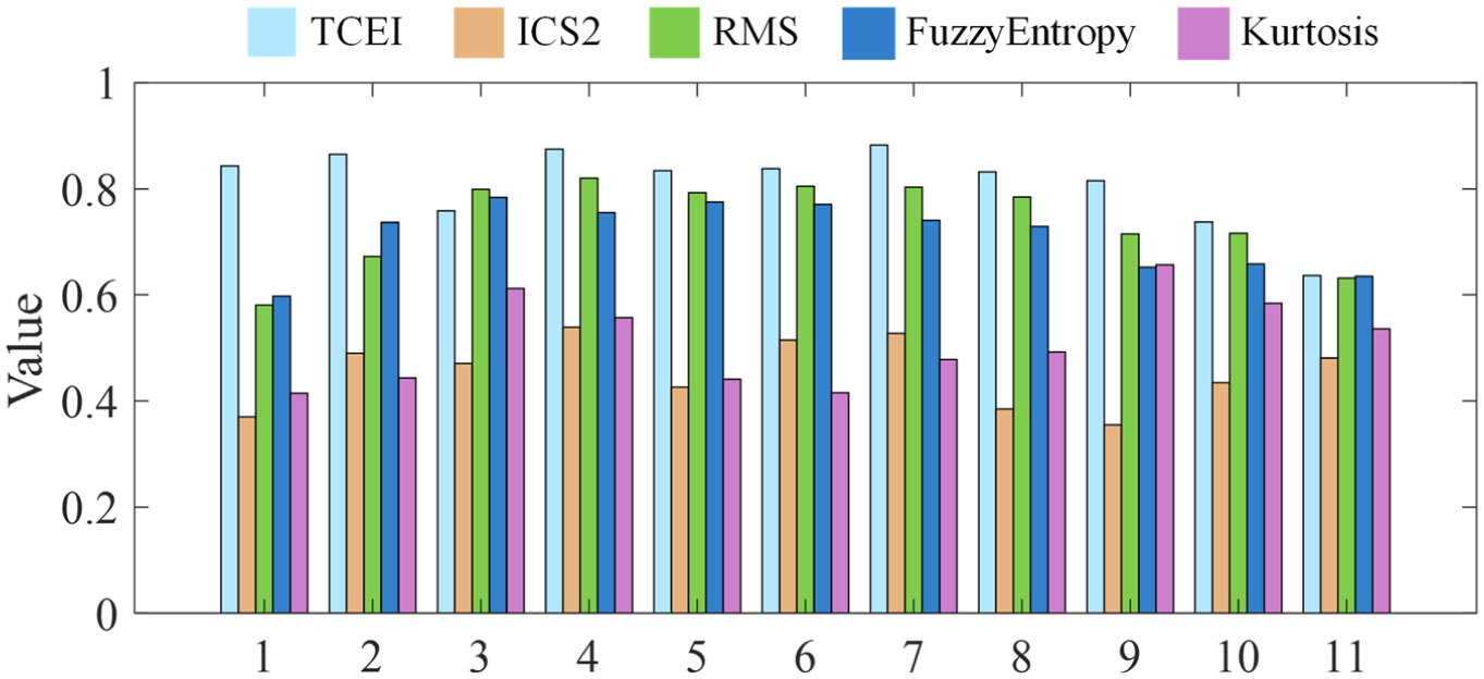
Comprehensive indicators.
For an intuitive comparison of degradation trends, datasets Test3 and Test4 were selected to visually compare the health curves of the TCEI against the benchmark indicators, as illustrated in Figure 9. Integrating both quantitative and qualitative analyses, it is evident that the TCEI achieves a higher composite metric than the four benchmark indicators. Furthermore, its degradation curve clearly reveals the multi-stage characteristics of the equipment, demonstrating superior correlation and degradation discernibility compared to the benchmark indicators.
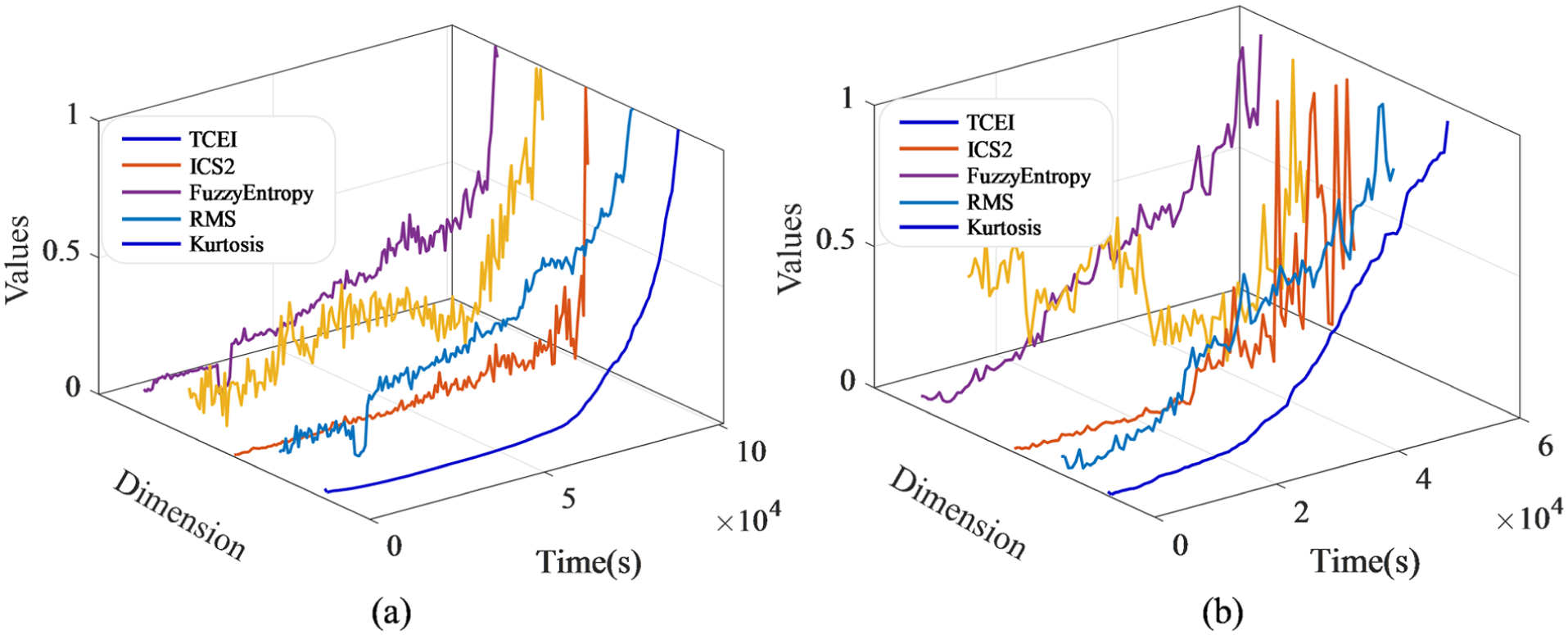
Indicator comparison: (a) Test3 and (b) Test4.
RUL prediction and comparative experiment
TCEI and four types of mainstream HIs were used as input features, respectively, and fed into SALNN for RUL prediction comparison experiments to verify TCEI application performance in practical engineering scenarios. The prediction results are shown in Table 3.
Comparison of HI prediction results.
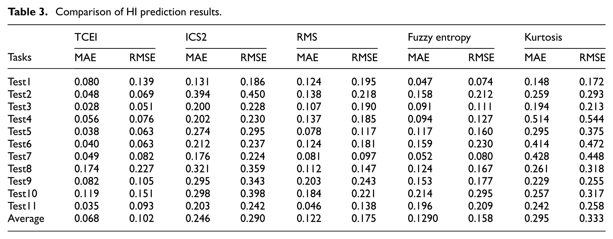
In prediction tasks involving 11 groups of harmonic drives, the model with TCEI as input achieved the highest average prediction accuracy and the optimal individual score in 8 of the groups. To visually demonstrate the predictive effect of TCEI, two units were selected, and their trajectories of RUL prediction are shown in Figure 10. The results indicate that TCEI has strong practicality in engineering applications.
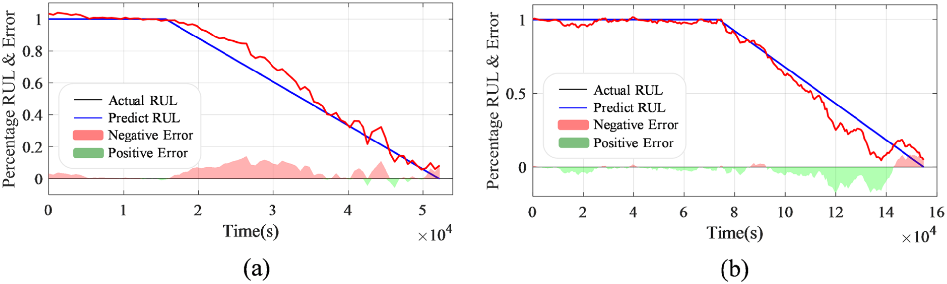
RUL prediction results: (a) Test4 and (b) Test6. RUL: remaining useful life.
In this section, a variety of representative models are selected for comparative experiments to verify SALNN’s performance. The comparative models fall into two categories: first, classical baseline models such as Bidirectional-Gated Recurrent Unit (Bi-GRU); second, state-of-the-art models that have performed well in RUL prediction in recent years, including MSTformer, 33 Dual Attention-Long Short-Term Memory (DA-LSTM), 30 Closed-form Continuous-depth neural-based hybrid difference Features Re-representation Network (CFC-F2RN), 47 Multilevel Focal Self-Attention (MLFSA), 37 and Slow Feature Analysis-Bidirectional-Long Short-Term Memory (SFA-Bi-LSTM). 20
The experimental results show that, across 11 groups of harmonic drives, SALNN achieves optimal prediction performance in most units. The average scores of the prediction results are shown in Table 4, and the average error of the proposed method is lower than that of all comparative models. The complete average experimental results are shown in Tables 5.
Prediction results of comparative methods.
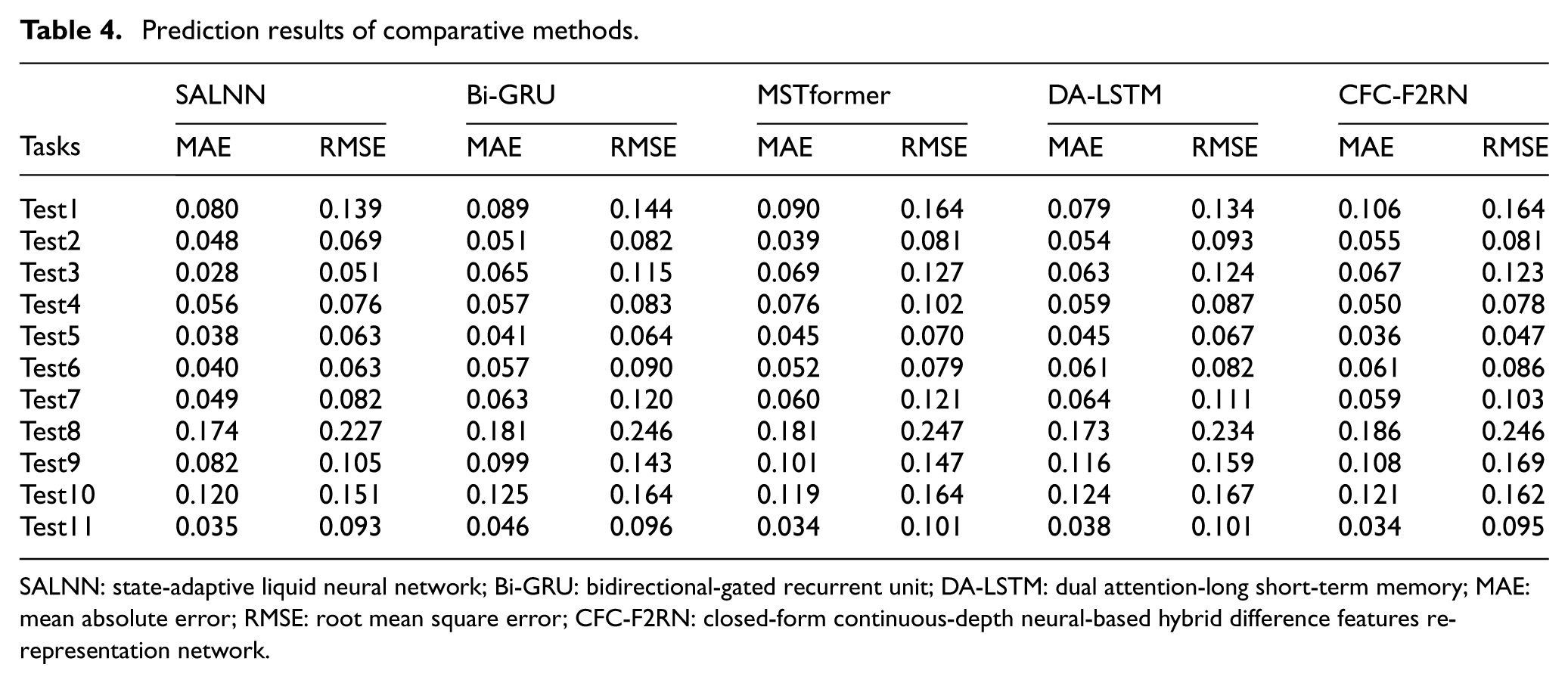
SALNN: state-adaptive liquid neural network; Bi-GRU: bidirectional-gated recurrent unit; DA-LSTM: dual attention-long short-term memory; MAE: mean absolute error; RMSE: root mean square error; CFC-F2RN: closed-form continuous-depth neural-based hybrid difference features re-representation network.
Average prediction results of comparative experiments.
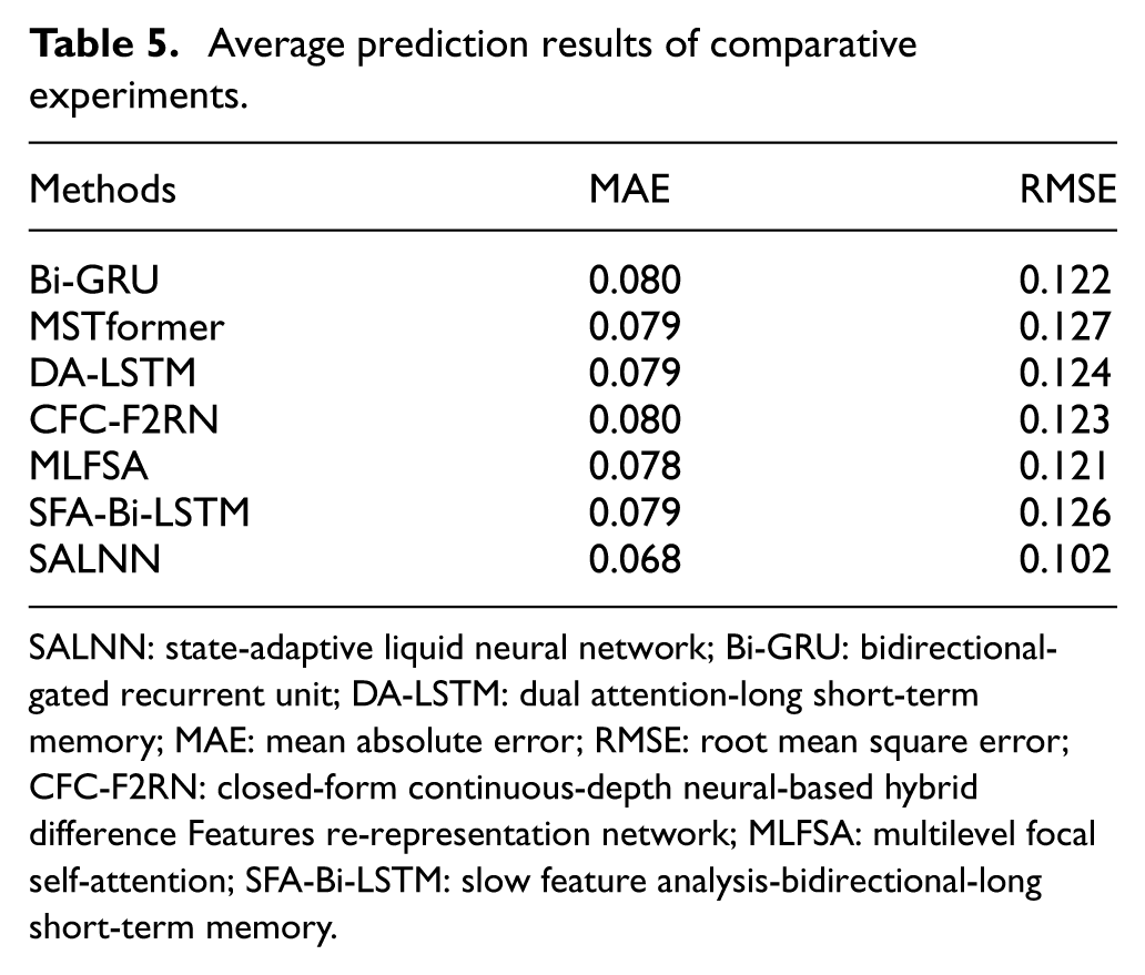
SALNN: state-adaptive liquid neural network; Bi-GRU: bidirectional-gated recurrent unit; DA-LSTM: dual attention-long short-term memory; MAE: mean absolute error; RMSE: root mean square error; CFC-F2RN: closed-form continuous-depth neural-based hybrid difference Features re-representation network; MLFSA: multilevel focal self-attention; SFA-Bi-LSTM: slow feature analysis-bidirectional-long short-term memory.
To intuitively demonstrate differences in prediction accuracy among models, four groups of units were selected, and three representative comparative models (MSTformer, DA-LSTM, and Bi-GRU) were selected. The RUL prediction trajectories under different network frameworks were visually compared with the actual degradation trajectories, and the results are shown in Figure 11. According to the results, the SALNN prediction trajectory closely matches the actual degradation curve of the harmonic drives.
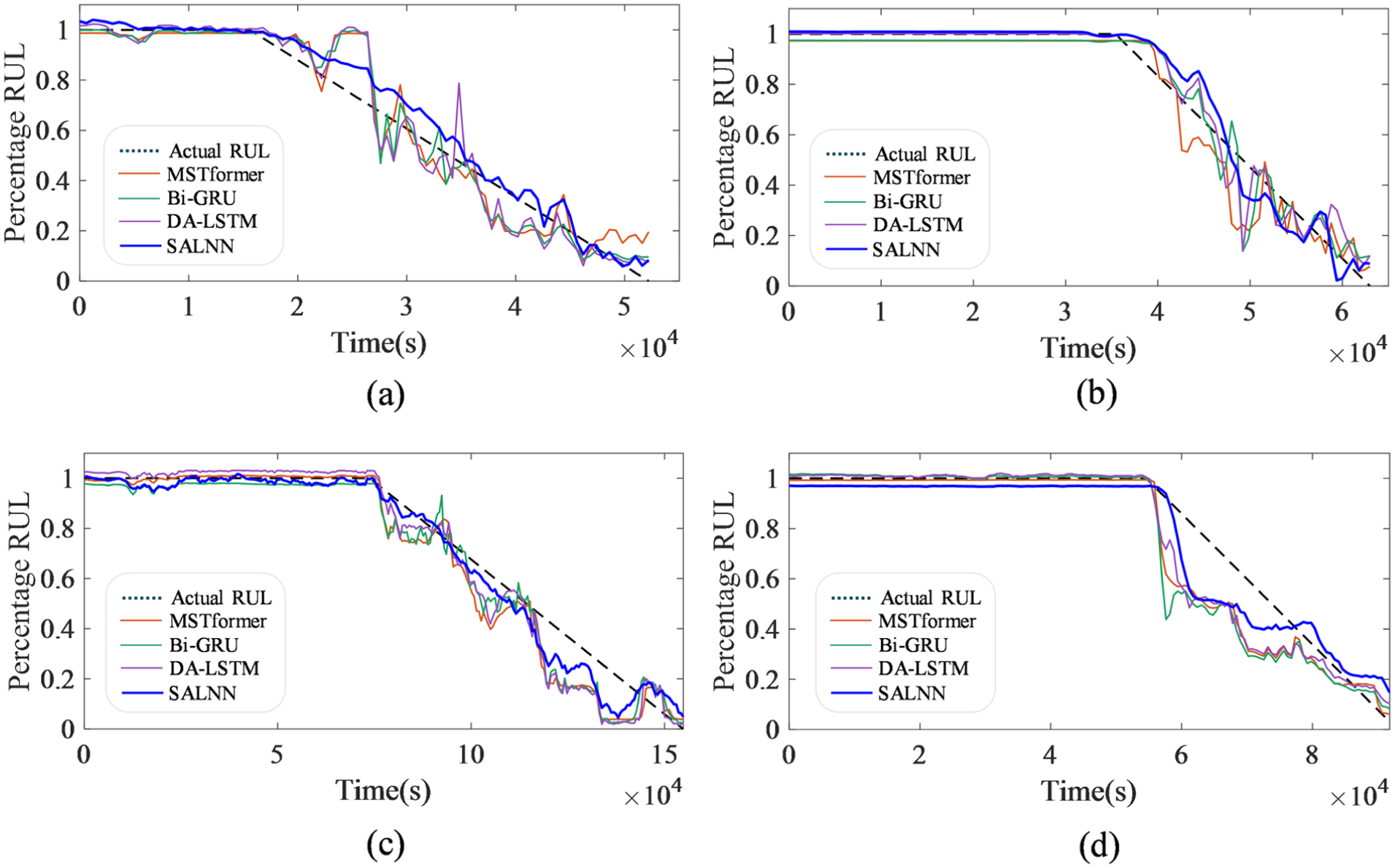
Comparative experiments: (a) Test4, (b) Test5, (c) Test6, and (d) Test7.
Ablation experiment
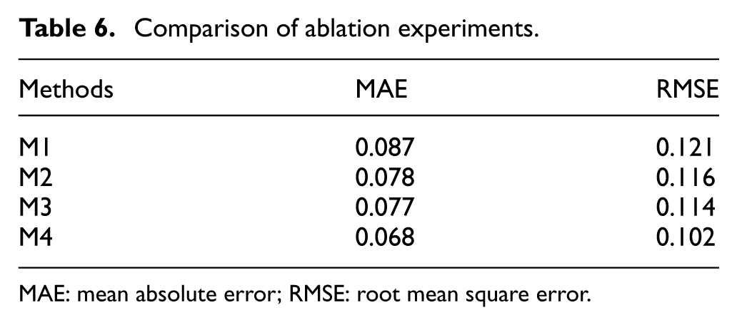
This section involved designing and conducting a series of ablation experiments to examine the impact of each module in the proposed method. In the model proposed above, a LayerNorm layer from the Transformer module was introduced at the end of the output hidden unit of each LTCs cell to stabilize the cell; for this reason, in the ablation experiments, a comparative model with this LayerNorm layer removed was first constructed and named M1. Regarding the adaptive time- constant module in the model, two sets of comparative experiments were designed to explore its impact: the first set directly removed the time-constant module and simplified the entire network into an ODE network, named M2, while the second set used a traditional liquid time-constant network, called M3. The complete model proposed in this article was designated M4 and served as the performance benchmark.
The RUL prediction results of the four methods (M1–M4) are shown in Table 6. A comparative analysis reveals that M4 achieves better predictive performance than the others. M1 experienced multiple gradient explosions during training, leading to extremely unstable final predictions, fully verifying the key role of LayerNorm in maintaining model stability. As M2 removes the adaptive time-constant module, its structure is overly simplified, failing to capture the equipment’s nonlinear degradation process accurately. In contrast, M3 adopts a complex liquid time constant, leading to large fluctuations in prediction results. This indicates that the complexity of the time constant is not positively correlated with performance; overly complex designs may, in fact, make the model more susceptible to short-term signal fluctuations.
Comparison of ablation experiments.
MAE: mean absolute error; RMSE: root mean square error.
Parameter discussion
This section designs controlled experiments to investigate the impact of model key parameters, focusing on three types: the hidden layer dimension of ODE cells, the batch size, and the sequence length. For each parameter, an average was calculated from 10 independent experiments to obtain the final result. For the remaining parameters, the liquid neural network is constructed with three layers and employs the Rectified Linear Unit (ReLU) function as the activation function.
The hidden layer dimension directly determines the model feature expression and memory capabilities, and its value is crucial to prediction accuracy. When the dimension is small, the model fitting ability is insufficient, making it challenging to extract deep features. When the dimension is large, the model complexity and computational cost increase, and overfitting may also occur. For this reason, four different hidden layer dimensions were selected for comparative experiments, and the prediction results are shown in Figure 12. Analysis shows that when the hidden layer dimension is set to 64, the model achieves the smallest prediction error. Batch size is the number of samples used to update parameters in each iteration, and it must balance computational efficiency with model stability. As shown in Figure 12, when the batch size is set to 32, it ensures stable parameter updates. The sequence length is the size of the input to the model during a single training session. Its size affects the ODE iteration process on the data, thereby influencing the extraction of degradation features. Four different sequence lengths were selected for comparative experiments in this article, and the results are shown in Figure 12. Research suggests that setting the sequence length to three results in the model’s best prediction performance.
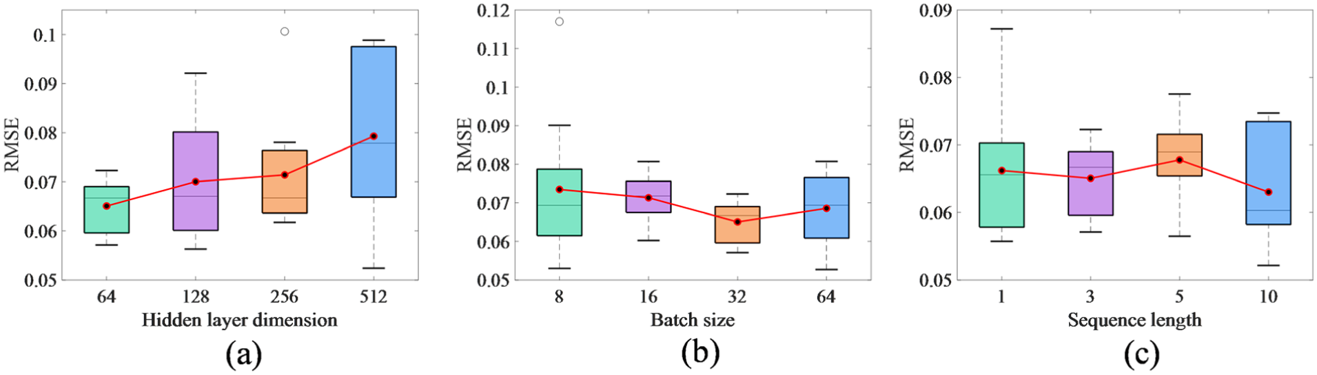
Parameter controlled experiments: (a) hidden layer dimension, (b) batch size, and (c) sequence length.
State detection and time-constant analysis
As a basis for adaptive time-constant allocation, accurate condition monitoring affects time constant regulation. The network architecture parameters of state discriminator and the RUL prediction layer are shown in Table 7.
Network architecture parameters.
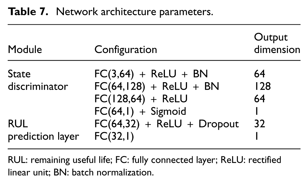
RUL: remaining useful life; FC: fully connected layer; ReLU: rectified linear unit; BN: batch normalization.
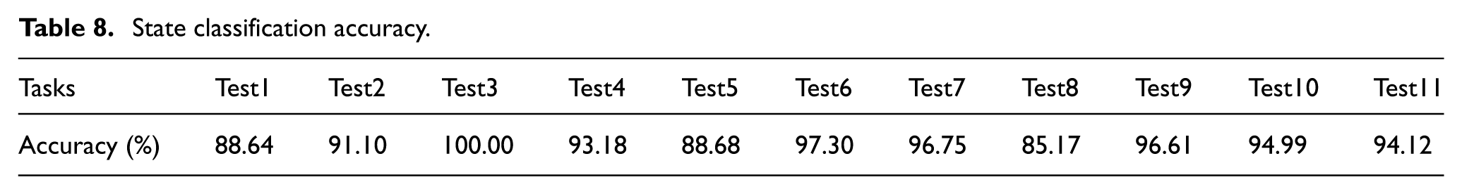
To verify the condition discriminator performance, the discriminator health probability output was compared with the actual degradation trajectory. The classification results for each dataset are shown in Table 8.
State classification accuracy.
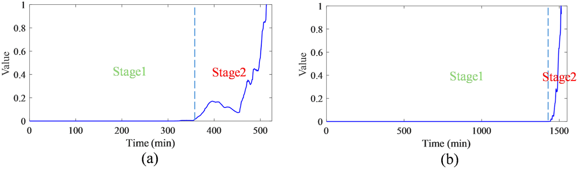
Using the Test3 and Test6 datasets as cases, the results are shown in Figure 13: the red curve represents the equipment health-state probability predicted by the model, the blue curve represents the actual RUL degradation trajectory, and the background colour indicates the model’s state classification results via binarization. The result shows that the condition discriminator accurately identifies the health state transition points, and the output health probability is consistent with the actual degradation trend, ensuring accurate regulation of the time constant.
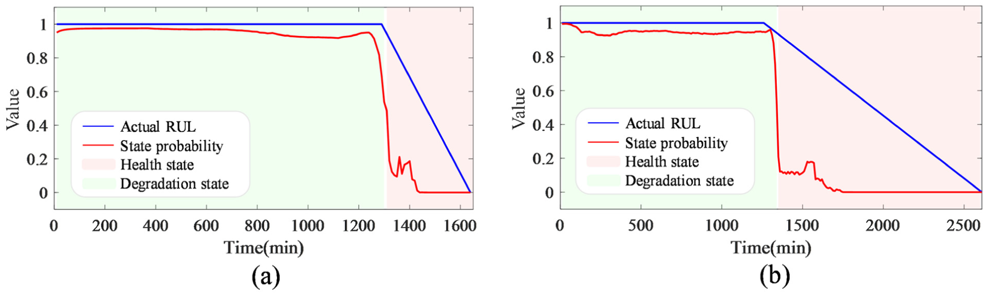
State classifications: (a) Test3 and (b) Test6.
Case 2: XJTU-SY dataset
Dataset description
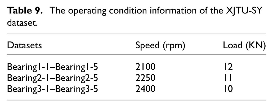
The second case study utilizes the rolling bearing dataset from Xi’an Jiaotong University. 48 This dataset was collected through accelerated degradation experiments on 15 bearing test units under three different operating conditions, comprehensively recording vibration signals from initial healthy operation to complete failure. For each operating condition, five parallel bearing test units were arranged to ensure data reliability. Detailed parameters for each operating condition and the corresponding bearings are presented in Table 9. The experimental platform structure, shown in Figure 14, consists of test bearings, a rotating shaft, an AC motor, a speed controller, support bearings, and a hydraulic system, simulating real-world bearing operation scenarios. The signal acquisition parameters were set as follows: a sampling frequency of 25.6 kHz, with vibration data collected for 1.28 s/min, ensuring complete capture of state characteristic changes throughout the bearing degradation process.
The operating condition information of the XJTU-SY dataset.
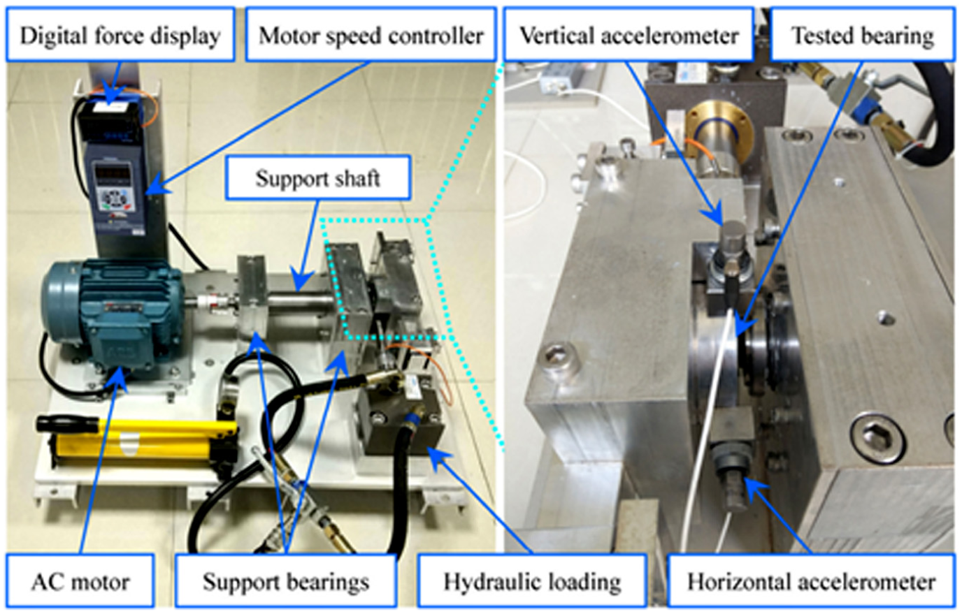
Rolling bearing test platform.
For model training and validation, the leave-one-out method was adopted. Each time, 1 of the 14 subsets was selected as the test set, while the remaining 13 served as the training set. Within the training set, an 11:2 ratio was further used to partition the data into training and validation subsets, aimed at optimizing model parameters and mitigating overfitting.
Selection of cycling frequency and fault frequency band
For the selection of parameters related to dataset, the vibration signals from the Bearing2_3 dataset Figure 15(a) were selected for analysis as an example. By substituting structural parameters into calculations, the outer race fault characteristic frequency was determined to be 107.91 Hz. From the spectral correlation diagram Figure 15(b), a significant energy concentration at the outer race fault characteristic frequency can be clearly observed; further, the MFP algorithm was applied to the cyclic frequency slices, accurately locating the target fault frequency band where energy is concentrated. For bearings under other operating conditions, the relevant fault frequencies were calculated first, and then the MFP algorithm was used to locate the target fault frequency bands Figure 15(c). Through this process, the relevant parameters can be determined.
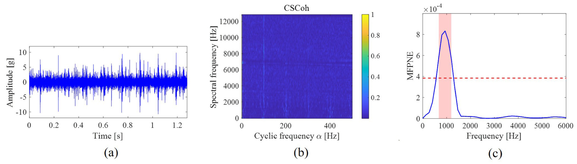
Bearing1_1 vibration analysis: (a) time domain signal, (b) spectral correlation, and (c) frequency band selection.
TCEI
To capture the degradation trend of bearings and accurately reflect degradation characteristics, the selected parameters are substituted into the formula to perform targeted energy feature extraction on each segment of the collected vibration signals. The extracted TCEI is an energy indicator that shows a sharp increase as faults become more severe. For better visualization, the HIs of the two bearing datasets (Bearing2_3 and Bearing3_4) after TCEI extraction are partially truncated, and the TCEI values for the final several time steps are not displayed initially. However, the full-life cycle data are used as input during RUL prediction, ensuring the model training process remains unaffected. As shown in Figure 16, the TCEI of both devices demonstrates clear multi-stage characteristics: the energy remains low during the first half of the service life, indicating a healthy state, while it shows an upward trend in the latter half, reflecting gradual degradation leading to failure, thus effectively representing the degradation progression.
TCEIs: (a) Bearing2_3 and (b) Bearing3_4.
RUL prediction and comparative experiment
To determine the effectiveness of the proposed indicator and model, the SALNN was compared with multiple RUL prediction methods using the dataset. The results of these methods are presented in Table 10. The proposed method achieves higher average prediction scores in terms of Mean Absolute Error (MAE) and Root Mean Square Error (RMSE) compared to other methods. Furthermore, the prediction results for the Bearing2_3 and Bearing3_4 datasets are shown in Figure 17 and the comparison results are shown in Figure 18.
Prediction results of comparative methods.
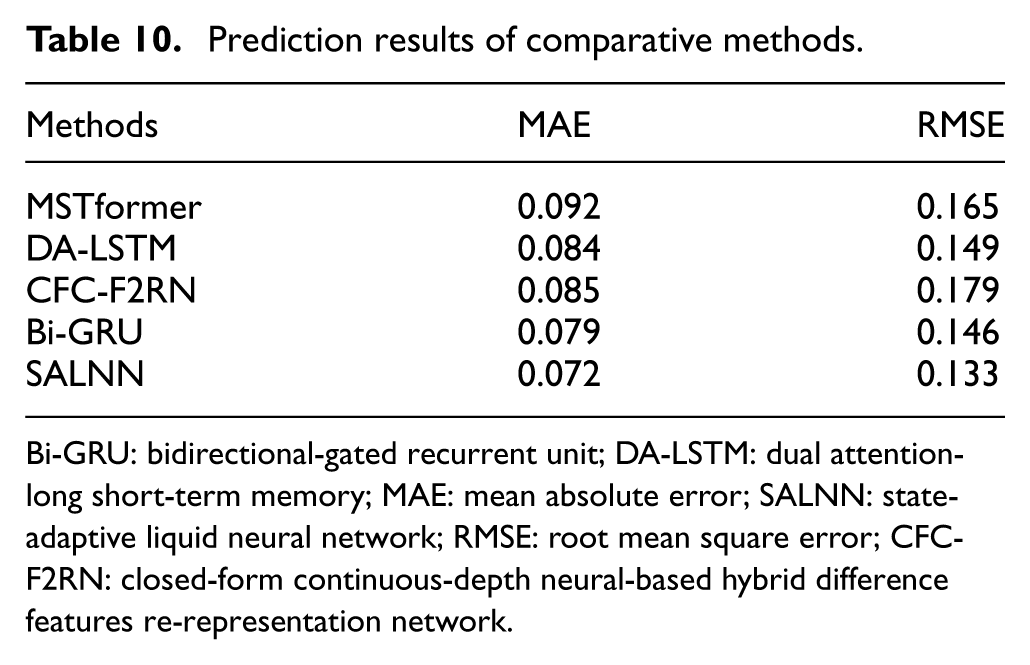
Bi-GRU: bidirectional-gated recurrent unit; DA-LSTM: dual attention-long short-term memory; MAE: mean absolute error; SALNN: state-adaptive liquid neural network; RMSE: root mean square error; CFC-F2RN: closed-form continuous-depth neural-based hybrid difference features re-representation network.
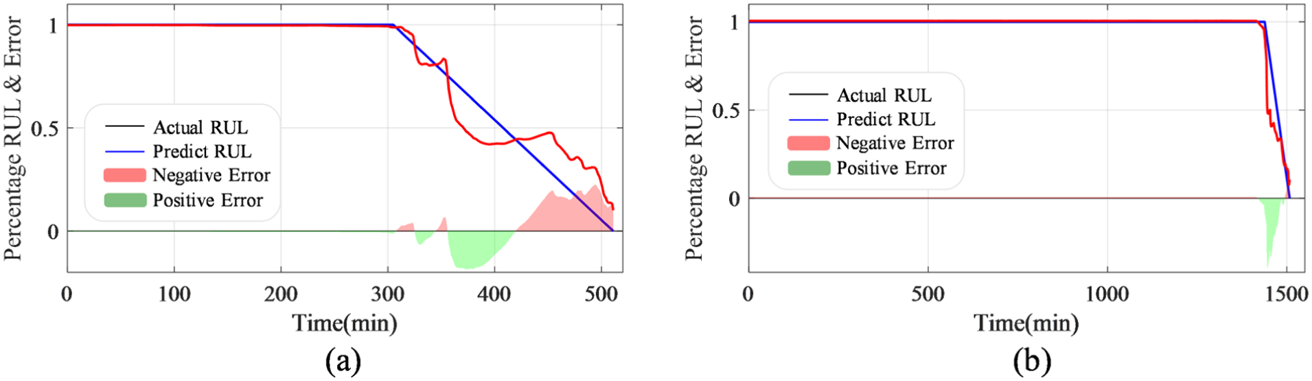
RUL prediction results: (a) Bearing2_3 and (b) Bearing3_4. RUL: remaining useful life.
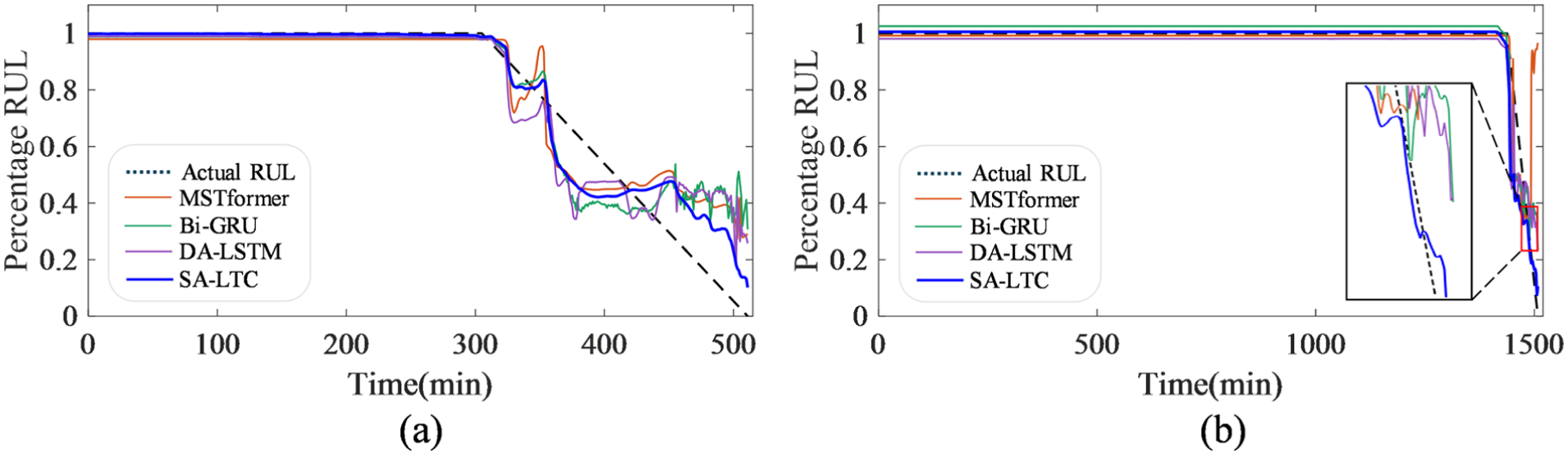
Comparative experiments: (a) Bearing2_3 and (b) Bearing3_4.
Conclusion
This article proposes a novel HI and an ODE neural network that integrates the degradation mechanism of harmonic drives. The TCEI constructed based on second-order cyclostationary characteristics exhibits multi-stage performance and anti-interference capability, allowing for efficient adaptation with the ODE neural network. The segmented time-constant in SALNN model compensates for the shortcomings of the traditional LTCs framework in RUL prediction, enabling it to accurately mine degradation trend features. A LayerNorm layer is introduced into the ODE cells to suppress gradient fluctuations, and the network is embedded in a bidirectional architecture to enhance feature extraction capability. Verification on the harmonic drive dataset confirmed the effectiveness and generalization ability of the indicator and the model. Compared with existing methods, the proposed TCEI indicator and SALNN model demonstrate significant advantages, providing support for the engineering deployment of online training and offline prediction, and laying theoretical and experimental foundations for the subsequent development of mobile detection technology.
However, the method proposed in this study is currently limited to relatively simple short-term forecasting scenarios and does not yet support transfer learning, continual learning, or forecasting for other, more complex tasks. Future work will incorporate these models into the framework and pursue more in-depth investigations on this basis.
Footnotes
Funding
The authors disclosed receipt of the following financial support for the research, authorship, and/or publication of this article: This research is supported by the National Natural Science Foundation of China under grant 52305089 and grant 52235002, and the Development Project of Beilun District under grant 2024BLG009, which is highly appreciated by the authors.
Declaration of conflicting interests
The authors declared no potential conflicts of interest with respect to the research, authorship, and/or publication of this article.