
Abstract
In actual operation, vibration signals from gearbox systems are susceptible to load fluctuations, speed variations, and environmental noise. The spectral differences between various fault states are often subtle, resulting in blurred sample boundaries and posing challenges for structural separation and state analysis. To address the aforementioned issues, this paper establishes a three-dimensional (3D) feature structure analysis framework based on frequency-domain statistical characteristics to investigate the structural distribution properties of gearbox vibration data. First, extract frequency-domain statistical features such as dominant frequency, energy, and bandwidth to construct a feature matrix. We then analyze the distribution patterns of different features in the sample space through two-dimensional projection analysis, identify key features that contribute significantly to the structure, and, by considering the correlations among features, perform structural consolidation and weighted fusion of features with similar trends to reduce the impact of redundant information on structural representation. Based on this, a 3D feature space is constructed to visualize the distribution patterns of samples under different operating conditions, and the structural separability is verified using the contour coefficient and various clustering methods. Experimental results demonstrate that, using field data and publicly available datasets that include various rotational speeds and multiple types of component failures, samples of different failure states all form distribution structures in 3D space characterized by clear boundaries and intra-class compactness, with contour coefficients all exceeding 0.92. Furthermore, the extracted feature sets exhibit a certain correspondence with fault vibration characteristics, indicating that this method is capable of effectively capturing the structural differences between various fault states under complex operating conditions. This provides a reliable feature foundation for gearbox system condition assessment, fault diagnosis, and subsequent intelligent recognition.
Keywords
Introduction
In recent years, the gearbox system, as a key power unit in industrial equipment, is widely used in the fields of transportation, aerospace, machinery manufacturing, energy equipment, and so on, and its operation status directly affects the reliability and efficiency of the whole machine.1,2 With the development of equipment in the direction of high power density, high speed, and long life, the operational safety and fault diagnosis ability of gearboxes have become an important link to ensure the stable operation of equipment.3,4 Under the action of complex load and alternating torque, the gear meshing pairs and their bearings and other components are prone to wear, pitting, tooth breakage, and other early damage. The degradation process is often subtle and progressive. If not promptly identified and addressed, it may further impair transmission performance, potentially leading to system shutdowns and resulting in economic losses or safety risks. Gearbox system failures are the focus and difficulty in the maintenance of industrial systems because of their hidden nature and fast propagation.5,6
Engineering sites are typically characterized by frequent changes in rotational speed, significant load fluctuations, and highly non-stationary signals, while the collected data often lacks clear annotation, which imposes certain limitations on fault identification methods that rely on empirical features or supervised models in practical applications. 7 Under the coupled effects of complex loads and multi-source excitation, the frequency-domain responses of different fault states often exhibit a certain degree of structural superposition. The spectral differences between multiple types of minor faults are relatively weak, and the distribution of samples in the feature space is prone to overlap. 8 The crux of this type of problem lies not in the difficulty of feature extraction, but in the fact that statistical features in the frequency domain often exhibit strong correlations and structural coupling. If dimension reduction or clustering is performed directly, it can easily lead to feature overlap, making it difficult to accurately capture the true differences between different states. In the engineering context where the spectral differences among various gearbox system failures are not pronounced and sample labeling is limited, how to clearly reveal the structural relationships among samples while maintaining the stability of the sample space distribution has become a problem that needs to be addressed in practical applications.9,10
In recent years, researchers both domestically and internationally have conducted extensive studies on vibration signal processing, feature extraction, and condition monitoring to address the challenge of fault condition analysis in gearbox systems under complex operating conditions. 11 Time-frequency analysis methods such as the fast Fourier transform (FFT), 12 Envelope Spectral Analysis, 13 and Wavelet Packet Decomposition 14 are widely used for fault feature extraction; Building upon this foundation, supervised models such as support vector machines, K-nearest neighbors, and random forests,15–17 along with related deep learning methods including convolutional neural networks, long short-term memory networks, and graph neural networks,18–21 have demonstrated strong classification performance on standard datasets. However, under real-world engineering conditions, labeled samples are often limited, and distribution shifts caused by varying operating conditions can also affect the generalization ability of supervised models. 22 In recent years, with the increasing prevalence of complex and unknown operating conditions, reliable and generalizable diagnostics have gradually emerged as key research areas in fault diagnosis. Related research has begun to focus on out-of-distribution testing, uncertainty assessment, and cross-condition generalization to improve the stability and reliability of models in practical applications. 23 In the absence of labels, unsupervised clustering methods such as K-means, density-based clustering (DBSCAN), and hierarchical clustering have been introduced for fault state classification.24–26 Concurrently, nonlinear dimensionality reduction algorithms like t-distributed stochastic neighbor embedding (t-SNE) 27 and uniform manifold approximation and projection (UMAP) 28 are employed to transform high-dimensional features into low-dimensional representations. From an engineering perspective, existing methods typically perform dimension reduction or clustering directly based on high-dimensional frequency-domain features, without fully accounting for the correlations and structural relationships among these features. Because statistical features in the frequency domain are often highly correlated, directly mapping them to a low-dimensional space can easily lead to structural aliasing; at the same time, under two-dimensional (2D) representations, samples from multiple fault classes tend to exhibit local crowding and overlap in the embedding space, making it difficult to fully capture their underlying distribution patterns. This makes it difficult to clearly distinguish between different operating states and complicates the identification of fault conditions under complex operating conditions. Therefore, how to more fully characterize the structural relationships among samples while maintaining the stability of spatial distribution has become a key challenge in fault analysis under unlabeled conditions. Based on the above analysis, in the context of high-dimensional frequency-domain features, how to preserve the complete representation of sample structural relationships in a low-dimensional space is one of the key issues determining whether effective separation can be achieved in fault state analysis under unlabeled conditions. 29 Compared to 2D representations, three-dimensional (3D) spaces have a greater capacity to capture structure; this can, to some extent, alleviate the crowding and overlap of samples during the dimensionality reduction process, allowing for a more complete representation of the distribution relationships among various fault types in the spectral space, and reducing the cross-contamination and misclassifications caused by 2D compression. In practical applications, the 3D space not only provides additional structural degrees of freedom but also facilitates the observation of sample distribution patterns from different viewpoints, providing a more intuitive basis for analyzing the patterns of state distributions. Building on this foundation, representing high-dimensional frequency-domain features as 3D structures and validating the sample distribution using simple and robust clustering methods helps yield clearer structural grouping results under unlabeled conditions, thereby providing a spatial foundation for subsequent state assessment and fault diagnosis. 30 Based on the above analysis, this paper proposes a frequency-domain feature analysis framework for 3D structural representation to address the issues of structural aliasing in gearbox systems under complex operating conditions and the significant differences in the contributions of various features to the sample space. By extracting frequency-domain statistical features such as center frequency, energy, and bandwidth, a normalized feature matrix is constructed, and, and by analyzing the distribution patterns of different features in the sample space using 2D projections, identify the key features that contribute most significantly to the structural unfolding; based on this, and taking into account the correlations among features, features with similar trends are consolidated and weighted to reduce the impact of redundant information on the structural representation. We then construct a 3D feature space to visualize the distribution patterns of samples in different operational states, thereby allowing the relationships between samples—which tend to overlap in a 2D space—to be more fully represented. Clustering methods are used solely as a means of structural validation to verify the structural separability of samples in 3D space, rather than as a final classification model, thereby providing structurally meaningful criteria for the assessment of gearbox system status and fault diagnosis.
Methodological framework and structural modeling
This method is based on the frequency-domain statistical characteristics of vibration signals and focuses on feature structure analysis, 3D structural representation, and structural validation. First, the original signal is segmented using the sliding window method, 31 and the time-domain signal is converted to the frequency domain using the FFT 32 to obtain the complete spectrum. The spectrum is composed of both the frequency axis and the amplitude distribution, where the frequency reflects the periodic characteristics of the signal and the amplitude portrays the energy magnitude of each frequency component. Extract typical statistical features such as center frequency, energy, and bandwidth to form a sample feature vector. To eliminate differences in feature dimensions and scales, the feature matrix is normalized column-wise. Building on this foundation, we further analyze the geometric distribution characteristics and structural relationships among the features to construct a weighted feature space for representing 3D fault structures and verify the separability of the sample space through 3D structural visualization and clustering results. Figure 1 illustrates the overall approach of the method described in this paper.
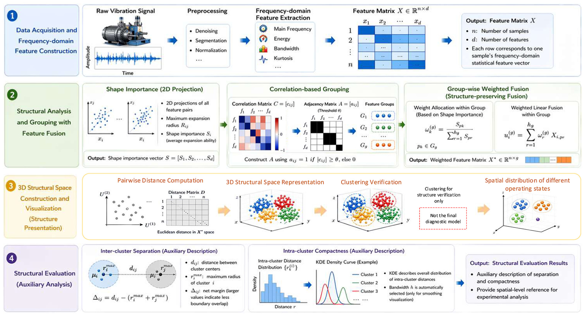
Framework for 3D fault structure analysis. 3D: three-dimensional.
Feature matrix construction
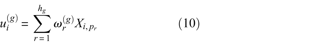
Building on the aforementioned preprocessing, we first establish a unified representation of the frequency-domain statistical characteristics of the vibration signals. For each segment of the vibration signal, we calculate typical statistical measures such as the dominant frequency, spectral energy, and bandwidth, and combine them into a d-dimensional feature vector in a fixed order. The feature matrix consisting of all the samples is denoted as X:
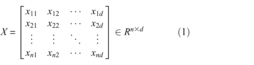
where n is the number of signal segments, d is the feature dimension, and each row corresponds to the feature vector of one sample. This matrix provides a unified description of the key statistical information of the vibration signal in the frequency-domain, laying the foundation for subsequent analyses of the geometric distribution of features, shape importance metrics, and 3D structural representation.
Inter-feature 2D projections and shape importance measures
After obtaining the normalized feature matrix
To describe this geometric contribution, in this paper, we use a two-by-two combination of features, where any two features (x i , x j ) are projected onto a 2D plane to form a point set Z ij :

where x
ki
and x
kj
denote the values of the kth sample on the ith and jth feature dimensions, respectively,
When a point cloud formed by combining a particular feature with multiple other features exhibits a large spatial extent, it indicates that this feature can increase the distance between samples in different directions, thereby fully resolving relationships between samples that would otherwise overlap easily, and thus making a greater contribution to the representation of the overall spatial structure. Therefore, the degree of geometric expansion in a 2D projection can serve as an important measure of the role of the structural features. To quantitatively characterize the shape of a 2D point set, its geometric center is first calculated:
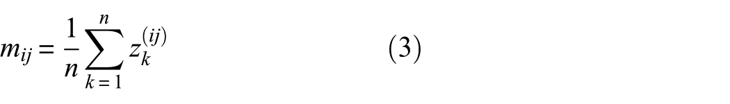
where

where
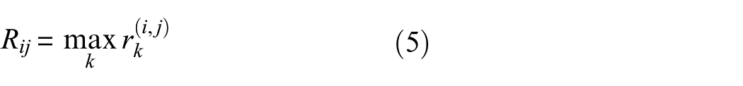
For all feature combinations, form the matrix
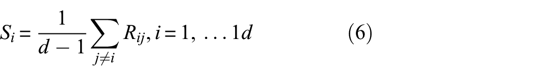
Here, S i represents the average expansion capability of the ith feature across different projection directions. This metric reflects the extent to which a feature contributes to the geometric structure of the sample space, rather than its ability to distinguish between categories in the traditional sense. Unlike statistical discriminant methods that rely on labels, shape importance is measured directly based on the distribution of samples, making it more suitable for structural analysis under unlabeled conditions. Furthermore, unlike manifold learning methods such as t-SNE and UMAP, which primarily preserve local neighborhood structures during the dimension reduction stage, the shape importance analysis proposed in this paper occurs during the high-dimensional feature construction stage. Its purpose is to identify key features that contribute significantly to the overall structure prior to dimension reduction, and to reduce structural overlap through subsequent feature fusion. These two methods operate at different levels—feature construction and spatial representation, respectively—and are not of the same type.
Inter-feature correlation structure identification and coupling relationship construction
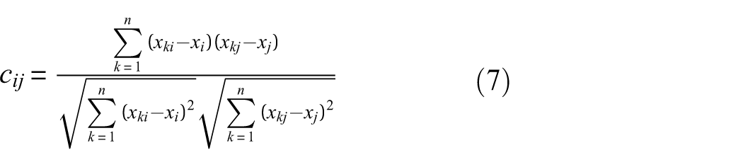
In the “Inter-feature 2D projections and shape importance measures” section, the shape importance metrics obtained from 2D projections characterize the extent to which features in each frequency domain contribute to the geometric unfolding of the sample space. Furthermore, to reduce structural redundancy among features and to preserve the main patterns of spectral variations represented by different features, it is necessary to identify which features exhibit consistent response patterns as the samples change, in order to determine whether they reflect the same or similar failure mechanisms. Frequency domain features are often not independent of each other in practical signal processing: Energy-type features often change as a whole with the degree of shock; the main frequency and its octave typically shift in phase with changes in rotational speed or load, while statistical measures related to the pulse components, such as bandwidth and kurtosis, may also show similar trends. This synchronous variation is not merely a mathematical correlation; rather, it reflects the shared response of different characteristics to the same physical process. Therefore, before representing the 3D structure, it is necessary to identify a set of features that vary in tandem in terms of statistical behavior, thereby avoiding the redundant description of similar spectral variation information by multiple features, which could otherwise affect the stable unfolding of the sample space structure. For this reason, this paper uses a linear correlation based on the overall trend of the sample to portray the synchronization between features. Let the feature matrix remain
where x
ki
and x
kj
are the values of the kth sample on the ith and jth feature dimensions, and
Based on the above calculation results, a correlation matrix
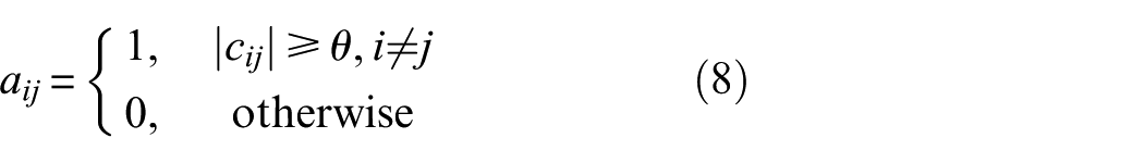
The adjacency matrix
Weighted fusion mechanism under feature coupling structure
In the “Inter-feature correlation structure identification and coupling relationship construction” section, frequency-domain features exhibiting synchronous variation patterns are grouped into several feature clusters through structural identification, such that each cluster primarily corresponds to the same type of spectral variation pattern. Although the same group of features shows similar trends in different working conditions, their contribution to the geometric structure of the sample space is not entirely consistent. Certain features are better able to distinguish between samples in a 2D projection and provide stronger support for the unfolding of spatial structures, while other features change in tandem with the features within the group; their contribution to distinguishing states is relatively limited. Therefore, further weighting within the group helps preserve the primary structural orientation and reduces the interference of redundant expressions on spatial organization.
Traditional feature weighting methods typically aim to improve classification accuracy by using label information to measure the importance of features and assigning greater weights to highly discriminative features. The weighted fusion described in this paper does not rely on class labels, and its purpose is not to improve the performance of a single classifier but rather to preserve the ability of samples to unfold their structure in a multidimensional space. In other words, weight allocation focuses on the contribution of features to the formation of geometric structures, rather than on classification ability in the traditional sense. Based on this, this paper uses the shape importance vector
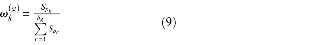
where p
k
denotes the column index of the kth feature in the gth feature cluster in the original feature matrix; p
r
denotes the column index of the rth feature in that feature cluster (for traversing all the features in the whole cluster); and
where
After fusing all g feature sets, resulting in the final weighted feature matrix X*

where
From a signal processing point of view, frequency-domain features often reflect the response process of the same failure mechanism in groups. For example, when the impact component increases, related statistical measures such as energy, bandwidth, and kurtosis typically increase in tandem; when the frequency components shift as a whole, the features near the fundamental frequency and its harmonics will also exhibit a consistent shift. By identifying key features within a group that make the primary structural contributions through shape importance analysis and assigning them higher weights during the fusion process, different failure mechanisms can be represented more independently and stably in the subsequent 3D space, thereby enhancing the separability and engineering interpretability of the sample distribution structure.
Construction of 3D structural spaces and presentation of failure modes
After completing the aforementioned feature construction, shape importance analysis, and intra-group weighted fusion, a weighted feature matrix X* with converged dimensions and reduced redundancy can be obtained. This feature space preserves the primary spectral variation patterns and their structural relationships; however, it remains difficult to directly observe the spatial distribution patterns among different samples based solely on the high-dimensional numerical form. To more intuitively analyze the structural relationships among samples from different operating states and to verify the effectiveness of the constructed feature space in mapping failure modes, this paper further conducts a 3D structural representation and visualization analysis. First, we use Euclidean distance to measure the relative differences among samples in the weighted feature space and construct a distance matrix between the samples. This matrix is used solely to describe the relative positions of samples in X* space; it does not involve any assumptions about categories. Its purpose is to provide a unified structural foundation for subsequent spatial representations. Based on this, the weighted feature space is mapped to a 3D structural space. This paper employs the t-SNE method to project high-dimensional sample relationships into a lower-dimensional space. Its purpose is not to serve as a core classification algorithm, but rather as a tool for visualizing 3D structures, enabling the observation of how samples are organized in the high-dimensional feature space. By preserving local neighborhood relationships, samples with similar spectral variation patterns remain relatively close to one another in 3D space, while samples with significant differences are gradually separated. This allows structural relationships that are difficult to observe directly in high-dimensional space to be visualized more intuitively. Compared to 2D representations, 3D space has a higher capacity for structural information, which can alleviate sample crowding and overlap during dimensionality reduction to some extent, making the boundaries between different fault states clearer. In particular, for samples with minimal spectral differences or localized overlaps, 3D structural representation offers greater spatial flexibility, enabling different failure modes to form more stable spatial distributions. After obtaining the 3D coordinates, we further employed clustering methods to validate the structure of the sample distribution. It should be noted that the clustering results are not intended to serve as the final fault identification model but are used solely to verify whether the samples form stable clusters in 3D space. By comparing the consistency of sample distributions across different clustering methods, we can determine whether the constructed feature space has achieved the structural characteristics of intra-class compactness and inter-class separation, thereby validating the effectiveness of the 3D structural representation. Through this process, the sample relationships corresponding to the frequency-domain features can be more fully represented in 3D space. This spatial distribution not only reflects the role of feature fusion in improving structural organization but also provides an intuitive structural basis for subsequent fault state analysis, thereby forming a comprehensive analytical process that spans feature construction, structural unfolding, and structural validation.
Metrics for evaluating cluster structures
To further examine the organizational patterns of sample distribution in 3D space, this paper introduces structural evaluation metrics based on geometric distribution to analyze the spatial separation between different clusters and the degree of clustering within each cluster. These metrics are primarily used to help describe structural features in 3D space and to determine whether samples from different operational states form relatively stable and distinguishable spatial distributions; they are not the sole criterion for assessing the validity of the method.
Interclass spatial separation
Inter-cluster separation is used to describe the relative distances between different clusters in 3D space. When different fault states form distinct clusters in space, there is typically a noticeable geometric distance between the clusters.
(1) Cluster center computing
For each class of sample points
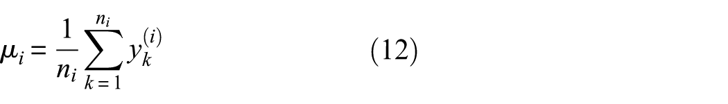
where μ
i
denotes the center coordinate vector of the ith cluster and n
i
is the number of samples in that cluster,
(2) Calculation of maximum class radius
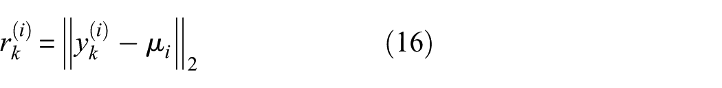
The distance from the center of a sample point within a cluster is defined in the two-norm:
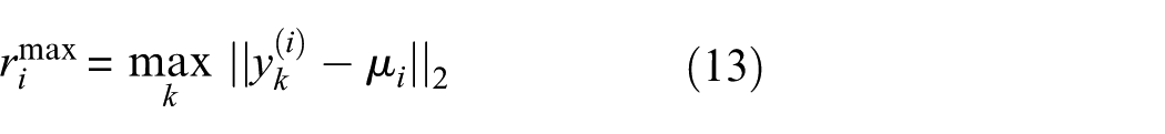
This value reflects the distance from the farthest sample in class i to the center, that is, the “maximum radius” of the cluster.
(3) Calculation of inter-cluster distance and net spacing
For any two different clusters i and j, the distance between their centers is defined as follows using two-norm:

The “net separation distance” between clusters is further defined as the distance between the centers of two clusters minus the sum of their maximum radii:
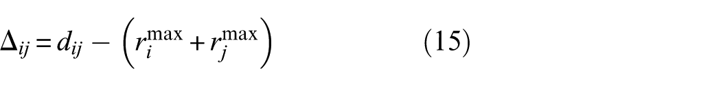
This metric is used to help visualize the boundaries between different clusters. When Δ ij is large, it indicates that the boundaries of the two clusters overlap little in space and that their distributions are relatively independent; when Δ ij is small, it indicates that the boundary distance between the two clusters is small, suggesting that the sample distributions may exhibit strong proximity and relatively weak spatial distinctiveness.
Compactness of class structures
In addition to inter-class separation, intra-class compactness is used to describe the degree to which samples within the same class cluster together in 3D space. If samples of the same type are concentrated in a specific area of space, this indicates that the fault state can form a stable structural region.
(1) Definition of distance within a class
For each class of clustered cluster C
i
, define the Euclidean distance between the kth sample point in the cluster and the center of the cluster as
where μ
i
denotes the center coordinate of the ith cluster, and
(2) Kernel density estimation methods
To characterize the overall distribution pattern of the radius within the class, this paper uses the kernel density estimation method to fit the probability density of
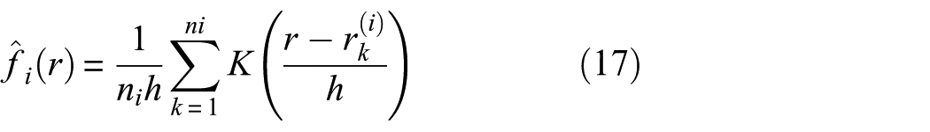
where K(⋅) is the Gaussian kernel function, h is the smoothing bandwidth (in this implementation, this parameter is automatically set to its default value by the “ksdensity” function; it is used solely to smooth the display of the intra-class radius distribution curve and does not contribute to the construction of the feature space or the generation of clustering results), r is the distance variable, and n i denotes the number of samples in the ith class. This method yields a continuous distribution curve of intra-cluster distances, allowing us to observe the degree of cluster cohesion.
If the distribution of intra-class distances is concentrated and the range of variation is small, this indicates that the samples are clustered closely together in space; conversely, if the distribution of distances is more dispersed, this indicates that the spatial structure of this class of samples is relatively loose.
This paper constructs a 3D structural space based on the geometric structure of frequency-domain features and performs a supplementary analysis of sample distribution patterns using inter-class spatial separation and intra-class structural compactness. These metrics are primarily used to observe the distribution patterns of different failure states in 3D space and to assess structural stability, thereby providing a spatial reference for the analysis of subsequent experimental results.
Fault data validation and structural analysis
The preceding section outlined the overall workflow for 3D fault structure analysis, focusing on the construction of frequency-domain statistical features, shape importance metrics, the identification of feature correlation structures, and weighted fusion methods. Building on this foundation, to verify the effectiveness of the constructed feature structure in real-world vibration signals, this paper conducts experimental analyses using both field-measured vibration data from construction sites and publicly available fault data from Southeast University.
Experimental data and feature settings
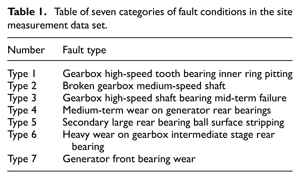
To analyze the applicability of the constructed feature structure under different signal conditions, this paper selected two representative vibration datasets as experimental subjects: the field-measured fault dataset and the Southeast University public fault dataset. The field measurement data originates from the equipment operation monitoring process at a wind power plant in Yunnan, China. Vibration signals were collected by sensors installed at critical locations. Because on-site equipment is constantly subjected to varying loads, fluctuating speeds, and ambient noise, the acquired signals exhibit distinct non-stationary characteristics, and spectral differences between various fault states are more susceptible to changes in operating conditions. This dataset includes seven types of fault conditions affecting critical components such as the high-speed shaft, medium-speed shaft, and bearings before and after the generator, and reflects changes in the vibration response of the transmission system under actual operating conditions. The various fault categories are shown in Table 1. It should be noted that type 1 through type 7 in Table 1 refer to the fault status codes corresponding to the raw data files; these are used solely to indicate the source of the samples and for cross-referencing subsequent results and are not included in the feature weighting, 3D embedding, or clustering processes.
Table of seven categories of fault conditions in the site measurement data set.
The Southeast University bearing failure dataset is a publicly available experimental dataset that includes four operational states: healthy, rolling element failure, inner ring failure, and outer ring failure. Compared to field measurement data, the acquisition environment for this dataset is relatively controlled and subject to minimal signal interference, making it suitable for validating fault diagnosis methods. This paper combines field measurement data with publicly available experimental data to evaluate the method’s performance on complex engineering data and to verify its applicability and stability across different data sources. The Southeast University fault dataset experimental platform is shown in Figure 2.
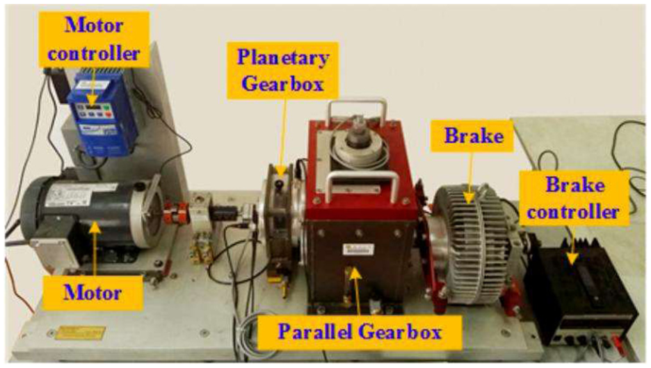
Southeast University fault dataset experimental platform.
For feature extraction, this paper employs a 12-dimensional set of frequency-domain statistical features derived from each vibration signal segment based on the previously established feature framework. These include fundamental frequency, spectral energy, bandwidth, spectral kurtosis, instantaneous frequency mean, harmonic ratio, spectral peak factor, spectral mean, spectral standard deviation, spectral skewness, spectral centroid, and spectral root mean square frequency. These characteristics describe the differences in fault signals in terms of frequency location, energy distribution, spectral shape, and impact components, providing a unified set of features for subsequent structural analysis. To minimize the impact of differing feature dimensions and numerical ranges on distance calculations, the feature matrix was standardized in the experiment to ensure comparability among features across different numerical scales.
Validation of field measurement datasets and structural analysis
Parameter settings and evaluation metrics
Based on the actual vibration data measured at the construction site, the experiment used the 12-dimensional frequency-domain statistical features described in the “Experimental data and feature settings” section as the initial input, and the feature matrix was normalized. The original signal has a sampling frequency of 1000 Hz. A sliding window method is used to divide the signal into segments, with a window length of 256 samples, an overlap length of 128 samples, and an adjacent window step size of 128 samples. After applying the sliding window method, approximately 200 sample segments are obtained for each fault state, resulting in a total of about 1400 sets of fault samples across the seven categories. After undergoing an FFT transformation, frequency-domain statistical features are extracted from each window signal for subsequent feature structure analysis and clustering validation. It should be noted that this paper does not introduce sample class labels during the clustering process; samples are grouped solely based on distance relationships in the feature space. In the experiment, the number of clusters is set based on the number of known operational states in the dataset to ensure that different methods are compared under the same number of categories; this does not imply that sample labels are used in feature construction or clustering calculations.
In the feature coupling and weighting stage, the feature correlation threshold θ and the t-SNE perplexity parameter 34 serve as the primary tunable parameters in this paper. In particular, the threshold θ is used to control the strength of the determination of synchronous relationships between features, which directly affects the number of feature groups formed after feature coupling; the perplexity parameter influences the extent to which t-SNE captures the scale of local neighborhoods during the low-dimensional embedding process. Based on the volume of data and the results of multiple experiments, this paper conducts combination tests on the aforementioned parameters within a reasonable range. The relevant threshold θ is searched for in the range [0.90, 0.98] with a step size of 0.01; the perplexity parameter is adjusted in the range [25, 75] with a step size of 5. For each set of parameter combinations, the processes of feature coupling, shape weighting, 3D structural representation, and clustering validation are performed, and the average contour coefficient of the corresponding results is calculated as an auxiliary evaluation metric. To minimize the impact of random initialization on the results, the experiment bound the random seed to the parameter combination and ran the clustering phase—which involves random initialization—20 times.
The contour coefficient is used to help evaluate the degree of intra-class clustering and inter-class separation in clustering results. It is defined as:
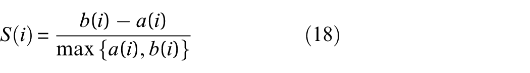
In the formula, a(i) represents the average distance between sample i and other samples in the same cluster, and b(i) represents the average distance from sample i to the nearest sample in another cluster. The shape coefficient S(i) takes values in the range [−1, 1]; the closer the value is to 1, the smaller the distance between the sample and the interior of its cluster, and the greater the distance between the sample and other clusters. In the experiments described in this paper, the contour coefficient is primarily used as an auxiliary metric for parameter combination screening and for comparing different feature representations; it is not the sole criterion for determining the validity of a 3D structure. Since t-SNE embedding results are primarily used for low-dimensional visualization, this paper does not interpret the geometric distance in the embedding space as a strict physical distance but rather as a basis for relative comparison among different feature representations under the same experimental conditions.
Comparative analysis of different feature representation methods
To verify the effectiveness of feature structure analysis and weighted fusion methods in improving the distribution of the sample space, this paper employs K-means clustering as a unified validation method to conduct a comparative analysis of the 3D structural results obtained under different feature representation methods. In this section, K-means is primarily used as a basic clustering tool to observe the distribution of samples in 3D space, rather than as a supervised fault detection model. By keeping the number of clustering categories and parameter settings constant, we can more directly compare the impact of different feature representations on spatial separation performance.
During the feature structure optimization process, the relevant thresholds and t-SNE confusion parameters have a certain influence on the final 3D structure. The experiment compiled data on representative combinations of parameters with higher profile coefficients and ranked them in descending order based on their average profile coefficients. The results are shown in Table 2.
Statistical results for combinations of high-profile coefficients based on field measurements.
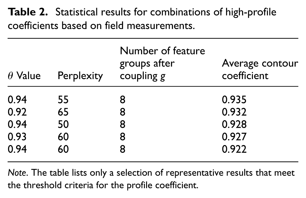
Note. The table lists only a selection of representative results that meet the threshold criteria for the profile coefficient.
As shown in Table 2, all of the representative parameter combinations listed achieved high average profile coefficients, and the differences in results between the various combinations were minimal. This indicates that the method described in this paper exhibits good stability with respect to the relevant threshold θ and the perplexity parameter. Although the parameter values differ, the number of effective feature groups after feature coupling remains at eight in all cases, indicating that the correlation structure among frequency-domain features is relatively stable and not merely a coincidence resulting from a specific set of parameters. Different combinations of parameters primarily affect the local embedding results without altering the overall structural relationships of the features. Based on the results of the overall profile coefficient and structural distribution, we subsequently selected θ = 0.94 and perplexity = 55 as the representative parameter combination for our method on the field measurement dataset.
To further illustrate the differences between the method described in this paper and traditional feature weighting approaches, Fisher weighting was introduced as a comparison in the experiments. It should be noted that Fisher weighting incorporates class information when calculating feature weights; therefore, in this paper, we use it solely as a baseline that incorporates class-based prior information for the purpose of comparing the differences between traditional discriminative weighting and the structural weighting fusion method proposed in this paper.
Based on this, 3D structural representations were generated for the original frequency-domain features, the Fisher-weighted features, and the weighted features constructed by the method proposed in this paper; the results of their spatial distributions are shown in Figure 3. It should be noted that the labels “type1” through “type7” in the figure are merely cluster IDs generated by the clustering algorithm or visualization labels and do not directly correspond to the original fault states “type 1” through “type 7” listed in Table 1. Fault names were not used as input during the clustering process; fault category information was used solely for interpreting the results after the experiment was completed.
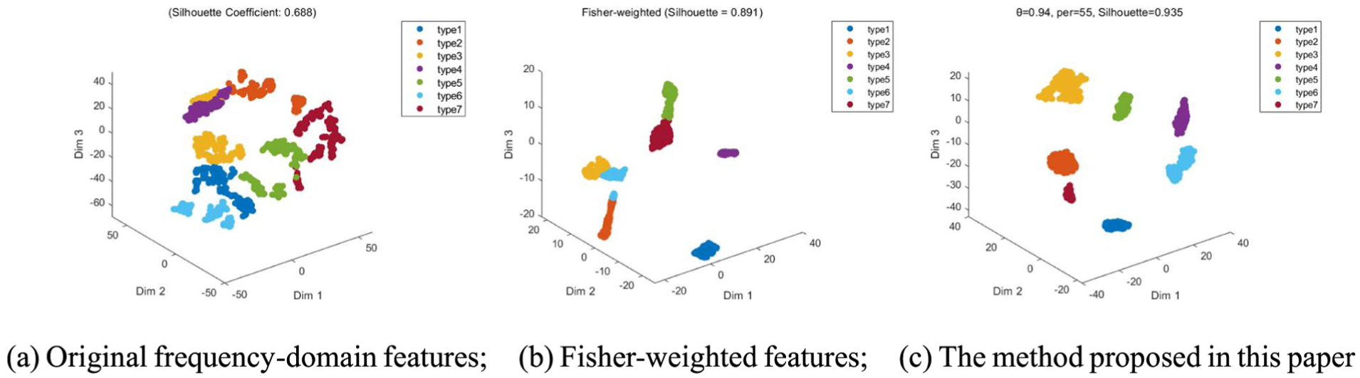
3D distribution of field measurement data using different feature representations: (a) original frequency-domain features, (b) Fisher-weighted features, and (c) the method proposed in this paper.
As shown in Figure 3(a), when the standardized original 12-dimensional frequency-domain features are used directly, the samples exhibit a certain degree of clustering, but the overall spatial structure remains relatively loose. Type 2, type 3, and type 4 are concentrated in the upper region, with relatively close spacing between clusters and localized adhesion at the boundaries; type 1 and type 6 are located in the lower region; although the two types of samples can be broadly distinguished, the spatial separation between them is insufficient; type 5 exhibits significant stretching in 3D space, with some samples extending into adjacent regions; the point cloud distribution for type 7 is also relatively dispersed. Its average contour coefficient is only 0.688, indicating that when raw frequency-domain features are directly incorporated into the 3D representation, they can reflect some differences in faults but struggle to form a stable, clear spatial structure. The primary reason for this phenomenon is that the 12-dimensional frequency-domain features contain not only useful information related to the fault state but also some redundant and weakly discriminative information. When features are treated equally during distance calculations and spatial embedding, key structural orientations are prone to distortion, leading to phenomena such as stretching, merging, and blurred boundaries in the sample point cloud. Figure 3(b) shows the results of the 3D structure after Fisher weighting. Compared to the original features, the overall distribution improved significantly after Fisher weighting. Types 1, 2, and 4 all formed relatively distinct clusters, the range of the sample point cloud narrowed compared to the results of the original features, and the average slenderness ratio increased to 0.891. This indicates that Fisher weighting can enhance features with strong discriminative power and plays a role in mitigating aliasing in the original feature space. However, as can still be seen in the figure, types 3 and 6 are relatively close in certain local areas, while types 5 and 7 are distributed adjacent to each other in the vertical direction; the boundaries remain unclear; at the same time, the point clouds for types 2 and 5 still exhibit some stretching, indicating that there is room for improvement in intra-class compactness. This is because Fisher weighting primarily assigns weights based on the inter-class differences and intra-class variability of individual features; while it can highlight certain discriminative features, it does not further address the redundant correlations among features. When multiple features exhibit similar spectral variation patterns, redundant information may still contribute to spatial embedding, causing certain categories to retain a clustered distribution or local clustering in 3D space. Figure 3(c) shows the 3D structural results obtained using the method described in this paper. It can be seen that the samples from the seven fault categories form distinct, independent clusters in 3D space, with clear separation between categories and no significant overlap. Compared with the results of the original features, the adhesion in the upper region was significantly improved for types 2, 3, and 4, while the tensile distribution for type 5 was effectively reduced; Compared to the Fisher-weighted results, the spatial boundaries between types 3 and 6, as well as between types 5 and 7, are more distinct, and the issue of clustering of certain categories has been alleviated. Although the point cloud coverage of type 3 is relatively large, it still maintains a clear spatial separation from other categories. The corresponding average profile coefficient reached 0.935, indicating that the method described in this paper achieves a better balance between inter-class separation and intra-class clustering.
The results above indicate that the improvements in the method described in this paper go beyond simply assigning different weights to features. Instead, the method first uses 2D projection to characterize the contribution of each feature to the geometric structure of the samples, then identifies sets of features that change in tandem based on these structures, and finally performs weighted fusion within each group. This process reduces the interference of redundant features on distance relationships while preserving the independent representation of key spectral patterns, such as the main frequency, energy distribution, and impact characteristics. Therefore, under complex operating conditions and in the presence of noise interference, different fault states can form a more stable spatial distribution in 3D space.
Combining the results in Figure 3 with the contour coefficient values, it can be seen that the average contour coefficients for the original features, Fisher-weighted features, and the method proposed in this paper are 0.688, 0.891, and 0.935, respectively, showing a gradual improvement. The results of the original feature analysis indicate that the direct use of multidimensional frequency-domain features is prone to being influenced by redundant and weakly correlated information; The Fisher-weighted results indicate that traditional discriminant weighting can improve the sample distribution, but it still does not adequately capture the structural relationships among features; The method described in this paper reconstructs frequency-domain features by considering both geometric contributions and relevant coupling structures, resulting in a clearer and more stable distribution of samples in 3D space. As can be seen, the structurally weighted fusion method is more effective at capturing the spatial differences between various fault states under complex operating conditions.
Comparative analysis of 2D and 3D structural representations
To further analyze the necessity of 3D structural representation, this paper maps the weighted features obtained using the proposed method to both 2D and 3D spaces via t-SNE under identical feature construction and parameter conditions and employs K-means clustering to provide supplementary validation of the sample distribution in the sample space. The corresponding results are shown in Figure 4, where Figure 4(a) shows the 2D structural results, Figure 4(b) shows the 3D structural results from the default view, and Figure 4(c) shows the 3D structural results from a rotated view.
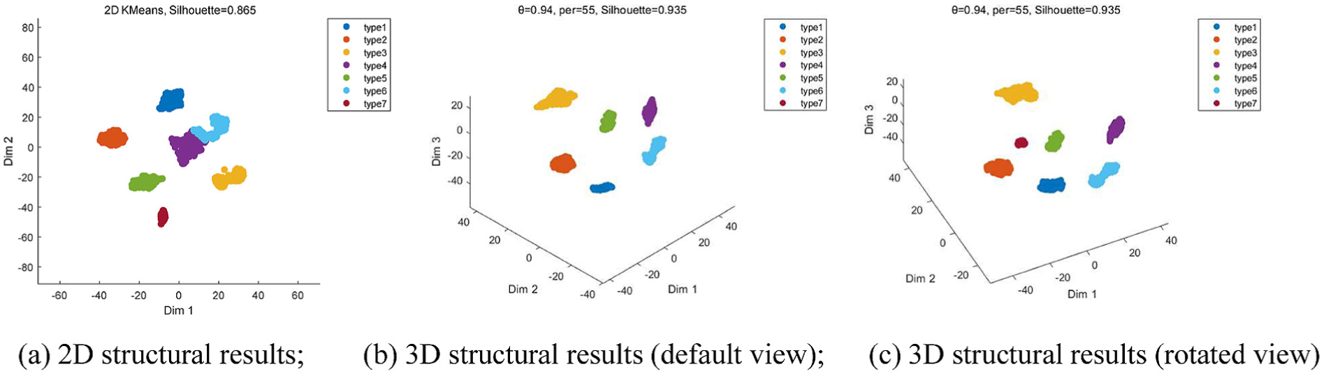
Comparison of 2D and 3D representations of field measurement data: (a) 2D structural results, (b) 3D structural results (default view), and (c) 3D structural results (rotated view). 2D: two-dimensional; 3D: three-dimensional.
As shown in Figure 4(a), most fault categories in the 2D structure have formed relatively distinct clusters; the spatial distributions of types 1, 2, 5, and 7 are relatively clear, and the samples within each category exhibit a certain degree of compactness. However, localized compression still occurs in the 2D plane. In particular, types 4 and 6 are located in the middle-right region of the figure; the two types of samples are relatively close to the boundary, and the point cloud of type 6 partially overlaps with that of type 4, which can easily create a visual overlap; although type 3 maintains a certain distance from other categories, its point cloud exhibits a locally dispersed pattern, and there is still room for improvement in terms of compactness. The average contour coefficient for these results is 0.865, indicating that the 2D structure can capture the basic distribution trends of the fault samples; however, it still struggles to fully represent the spatial hierarchy among samples in regions where categories are closely clustered. Figure 4(b) shows the results of the 3D structure obtained under the same conditions. Compared with the 2D results, the 3D space adds an additional dimension of representation, allowing sample clusters that were relatively close together in the 2D plane to spread out further along the third dimension. As can be seen, types 1, 2, 3, 4, 5, and 6 all form distinct clusters in 3D space. The local overlap between types 4 and 6 in the 2D plot has been significantly reduced, and the spatial distance between them is now more clearly defined. At the same time, the average contour coefficient of the 3D structure increased to 0.935, indicating improvements in both inter-class separation and intra-class clustering. It should be noted that, under the default viewing angle shown in Figure 4(b), type 7 is not clearly visible, which may give the impression that this class is missing or overlaps with other classes. Based on 3D spatial characteristics, it can be concluded that this phenomenon is primarily caused by front-to-back occlusion resulting from the viewing angle, rather than complete overlap of the samples in real 3D space. In other words, a 3D map created from a fixed viewpoint is still a projection; if structural distribution is assessed based solely on a single viewpoint, the actual spatial distances between certain categories may be underestimated. To further validate this, Figure 4(c) shows the 3D structure results from a rotated perspective. After rotation, it is clearly visible that the cluster of type 7 samples, which was previously obscured in the default view, has become visible and maintains a distinct spatial position relative to the surrounding categories. At this point, all seven classes of fault samples can be clearly observed in 3D space, with no significant overlap between the classes. In particular, the spatial relationship between type 7 and adjacent categories becomes clearer after rotation, indicating that it is not being confused with other categories but is simply obscured by objects in front of it from the default viewpoint. As can be seen, 3D representations allow for a more comprehensive visualization of the hierarchical relationships between samples, thereby further revealing the distribution of categories that are compressed or obscured in a 2D plane.
As can be seen from Figure 4(a) through (c), although 2D representations can illustrate the overall distribution of faulty samples, they are prone to the effects of planar compression under complex operating conditions, resulting in the boundaries of some categories becoming blurred or locally overlapping. 3D structural representation, by increasing spatial freedom, allows different fault categories to be more fully displayed in space and enables the observation of the actual distances between categories and the visual occlusion caused by projections through rotation. Therefore, the use of a 3D representation in this paper is not merely to enhance visualization but to more comprehensively illustrate the distribution of complex fault samples in the feature space.
Verification of structural stability under different clustering methods
To further validate the stability of the constructed 3D feature structure, this paper introduces hierarchical clustering and spectral clustering for comparative validation under the previously mentioned optimal parameter conditions. It should be noted that the focus of this section is not on comparing the merits of different clustering algorithms, but rather on examining whether, within the same weighted feature space, samples can maintain a relatively consistent spatial separation pattern under different clustering criteria. If a 3D structure is effective only for a specific clustering algorithm, this indicates that its stability is limited; If all clustering methods yield relatively clear distribution results, this further demonstrates that the feature space constructed in this paper possesses good intrinsic separability.
In the experiment, the parameter combinations determined in the “Comparative analysis of different feature representation methods” section were again used. Both hierarchical clustering and spectral clustering were performed on the 3D structural space obtained by the method described in this paper, and the results are shown in Figure 5.
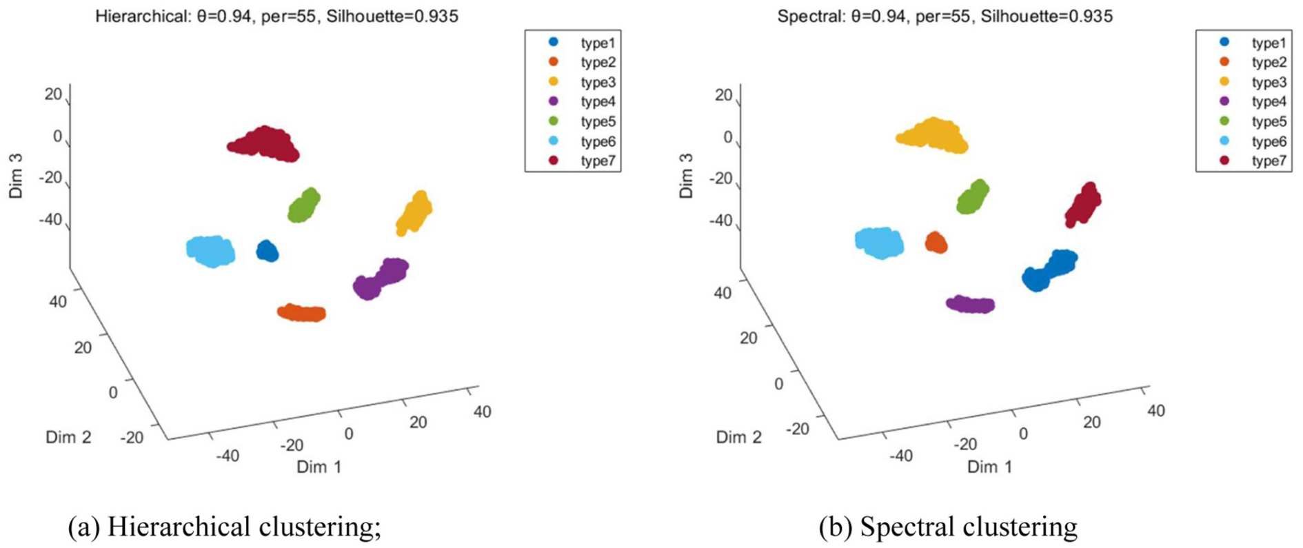
Results of 3D structure validation using different clustering methods based on field measurement data: (a) hierarchical clustering and (b) spectral clustering. 3D: three-dimensional.
As shown in Figure 5(a), after hierarchical clustering, the seven sample categories still form relatively distinct clusters, with clear spatial separation between them and no significant overlap. Some categories are relatively close to one another in spatial terms, but their boundaries remain fairly distinct, and there is no noticeable blurring within the point cloud. Hierarchical clustering primarily involves the gradual merging of clusters based on the distance relationships between samples, without relying on the assumption of centroid partitioning found in K-means. Therefore, these results indicate that the 3D feature space constructed in this study can still achieve good separation performance under a clustering method based on hierarchical distance relationships. Figure 5(b) shows the results of spectral clustering. It can be seen that, under spectral clustering, samples in each category still exhibit a relatively compact clustered distribution, with distinct gaps between clusters; the overall spatial pattern is largely consistent with the results of K-means and hierarchical clustering. Spectral clustering focuses more on the adjacency relationships and local connectivity structures among samples. These results indicate that the 3D feature space obtained by the method proposed in this paper not only exhibits good separability in terms of global distance distribution but also effectively preserves the differences between various fault states in terms of local neighborhood structures. It should be noted that both hierarchical clustering and spectral clustering are unsupervised classification processes; during clustering, only 3D coordinate information is used, without incorporating fault category information. The cluster labels generated by different clustering methods are used solely for display purposes; the order of these labels has no specific meaning. Therefore, the colors in the figure may not correspond exactly to the K-means results. This phenomenon merely reflects differences in the order in which numbers are displayed by different algorithms; it does not affect the interpretation of the spatial structure.
Overall, K-means, hierarchical clustering, and spectral clustering all yield relatively clear clustering structures in the same weighted 3D feature space. In particular, the average contour coefficient for K-means, hierarchical clustering, and spectral clustering was 0.935 in each case, indicating that the 3D structure is not dependent on any specific clustering criterion. In other words, clustering algorithms primarily serve a structural validation function in this paper; the fundamental reason why samples can be stably separated lies in the fact that the prior feature structure analysis and weighted fusion enhance the ability to express differences in the frequency domain.
3D structural analysis and explanation of failure mechanisms
To avoid relying solely on 3D scatter plots for qualitative interpretation of the results, this paper conducts a supplementary analysis of the 3D structure based on the K-means clustering results, taking into account the inter-cluster net distance, the distribution of intra-cluster radii, and the physical significance of the feature groups. It should be noted that C1∼C7 in this section refer only to the cluster IDs output by the K-means algorithm, which are used to describe the spatial distribution; they do not directly correspond to the original fault category IDs in Table 1. Figure 6 shows the results of the net inter-cluster distances between the clusters based on the field measurement data.
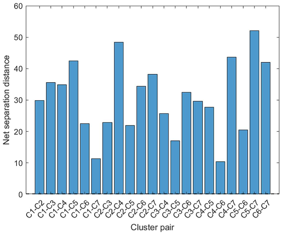
Net separation distances between clusters based on field measurement data.
As shown in Figure 6, the net inter-cluster distances are all positive, indicating that, in the current 3D structure, the clusters maintain an observable spatial separation from one another and do not overlap significantly. In particular, the distances between clusters such as C5–C7, C2–C4, C4–C7, and C6–C7 are relatively large, indicating that these states are well separated in 3D space; in contrast, the intervals between clusters such as C4–C6, C1–C7, and C3–C5 are relatively small, indicating that although these clusters are distinct, their boundaries are close together, and they still constitute a combination of states that are likely to produce similar frequency-domain responses. These results are largely consistent with the spatial distribution observed in the scatter plot presented earlier, indicating that the 3D structure obtained using the method described in this paper is not merely visually dispersed but also exhibits certain structural differences along the boundaries between clusters. Figure 7 further presents the kernel density estimates of the distances from samples within each cluster to the cluster center.
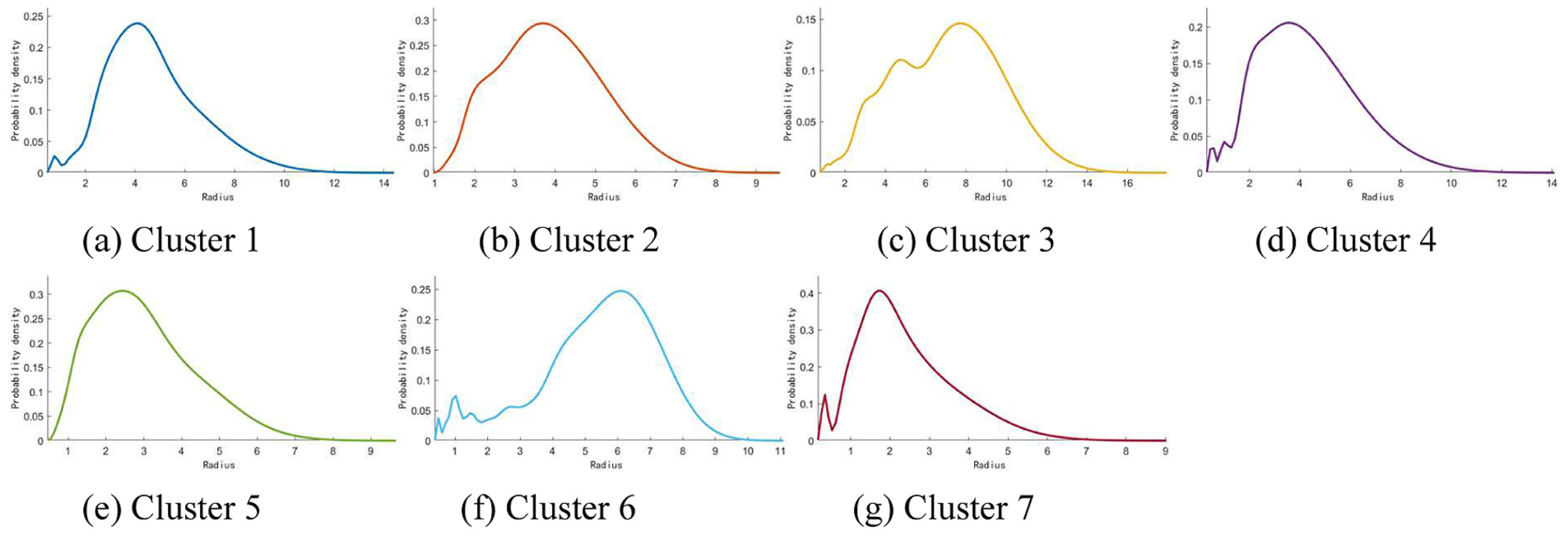
Distribution of kernel density within each cluster based on field measurement data: (a) cluster 1, (b) cluster 2, (c) cluster 3, (d) cluster 4, (e) cluster 5, (f) cluster 6, and (g) cluster 7.
As shown in Figure 7, the radius distributions of most clusters exhibit a single main peak or a cluster of main peaks, indicating that samples within the same cluster generally cluster around the central region. In particular, the peaks of the C5 and C7 curves occur relatively early and decline rapidly, indicating good compactness within their respective classes; The distributions of C2 and C4 are also relatively concentrated, with limited dispersion. In contrast, the radius distributions for C1, C3, and C6 are relatively broader, indicating that there is still some expansion within these sample categories. This phenomenon is related to the complexity of on-site measurement data: field signals are affected by fluctuations in rotational speed, changes in load, and ambient noise; even under similar operating conditions, there may be some variation in spectral amplitude, energy distribution, and impact components. Consequently, the distribution within certain categories may exhibit a relatively wide range of radii. In terms of feature structure, under optimal parameter conditions, the method described in this paper consolidates 12-dimensional frequency-domain features into eight feature groups, as shown in Table 3.
Composition and physical meaning of the characteristic groups in field measurement data.
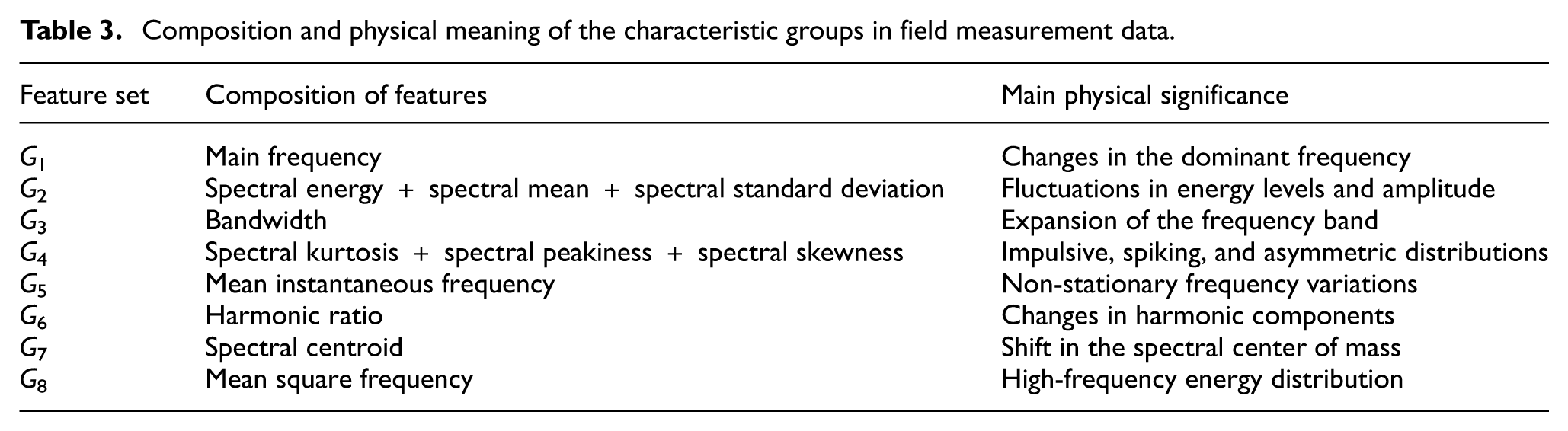
As shown in Table 3, the merged feature set is not a random combination but rather exhibits a clear correspondence with the spectral response of the fault vibration signal. G1, G6, G7, and G8 primarily reflect changes in the frequency structure, including information such as the location of the fundamental frequency, harmonic components, the center of gravity of the spectrum, and the distribution of high-frequency energy. When gear meshing abnormalities, shaft-related failures, or an increase in bearing characteristic frequency components occur, the spectrum typically exhibits changes in the fundamental frequency or harmonic components. Consequently, these features remain relatively independent in the clustering analysis, indicating that they serve as independent indicators of different operating conditions. G2 and G3 primarily describe changes in energy amplitude and bandwidth expansion. When equipment experiences faults such as wear, spalling, or fracture, the vibration energy and frequency spectrum often change; therefore, energy and bandwidth characteristics can reflect the overall increase in response caused by the fault. G4 is composed of spectral kurtosis, spectral peak factor, and spectral skewness and primarily corresponds to phenomena such as local impacts, peak enhancement, and skewed spectral distribution. It is consistent with the impact-type responses caused by bearing pitting, spalling, and localized damage in gears. G5 reflects frequency response characteristics under non-stationary conditions and is more sensitive to fluctuations in rotational speed and load variations in field data.
As can be seen from the above results, the feature sets obtained using the method described in this paper not only reflect the statistical correlations among the features but also preserve the primary response patterns of different failure mechanisms in the frequency spectrum. The frequency structure group, energy statistics group, bandwidth expansion group, and impact characteristics group describe the differences in fault signals from different perspectives, enabling the samples to form a relatively clear distribution structure in 3D space. When different faults exhibit significant differences in their impulse components, energy levels, or frequency structures, the corresponding samples are more likely to form compact and well-separated spatial clusters; when the spectral response patterns of certain faults are similar, the distance between their clusters is also relatively small. It should be emphasized that this paper does not equate the geometric distance in the t-SNE embedding space directly with actual physical distance, nor does it rely solely on 3D scatter plots as the basis for determining failure mechanisms. This paper uses 3D structural results as an auxiliary observational tool and interprets them in conjunction with the composition of feature groups and their corresponding spectral response mechanisms. This demonstrates that the separation observed in the 3D structure is not merely a result of visualization effects but is related to physical characteristics such as energy distribution, bandwidth expansion, impulse response, and changes in frequency structure under different fault conditions, thereby enhancing the engineering interpretability of the constructed 3D structure.
Validation using the Southeast University public dataset
To further evaluate the adaptability of the method described in this paper across different data sources, we selected the publicly available fault dataset from Southeast University for additional validation. This dataset includes four states: Ball fault, Healthy, Inner fault, and Outer fault, with a sampling frequency of 1000 Hz. The experiment used a sliding window method to partition the samples, with a window length of 2048 data points, an overlap length of 1536 data points, and a step size of 512 data points between adjacent windows, resulting in a total of 336 sample groups. Compared with field measurement data, this dataset was collected under relatively stable conditions with minimal noise interference; however, it differs in terms of fault types, sample size, and spectral distribution characteristics. Therefore, it can be used to evaluate the applicability of the method described in this paper under various data conditions.
The experiment continues to use the 12-dimensional frequency-domain statistical features constructed earlier as input, and the feature matrix is normalized. Given that the sample size of this dataset is smaller than that of the on-site measurement data, the parameter search range has been narrowed accordingly: The threshold θ is set to [0.94, 0.96] with a step size of 0.01; the t-SNE perplexity parameter is set to [15, 25] with a step size of 1. Under different parameter combinations, K-means, hierarchical clustering, and spectral clustering were used for validation. It should be noted that dimension reduction and clustering calculations use only the frequency-domain feature matrix; fault names are not included in the model calculations. The category names shown in the figure are used solely for labeling the results and explaining their engineering significance. Under optimal parameter settings, the method described in this paper consolidates the 12-dimensional frequency-domain features of the Southeast University dataset into nine feature groups; the specific results are shown in Table 4.
Results of feature grouping for the Southeast University dataset and their main physical meanings.
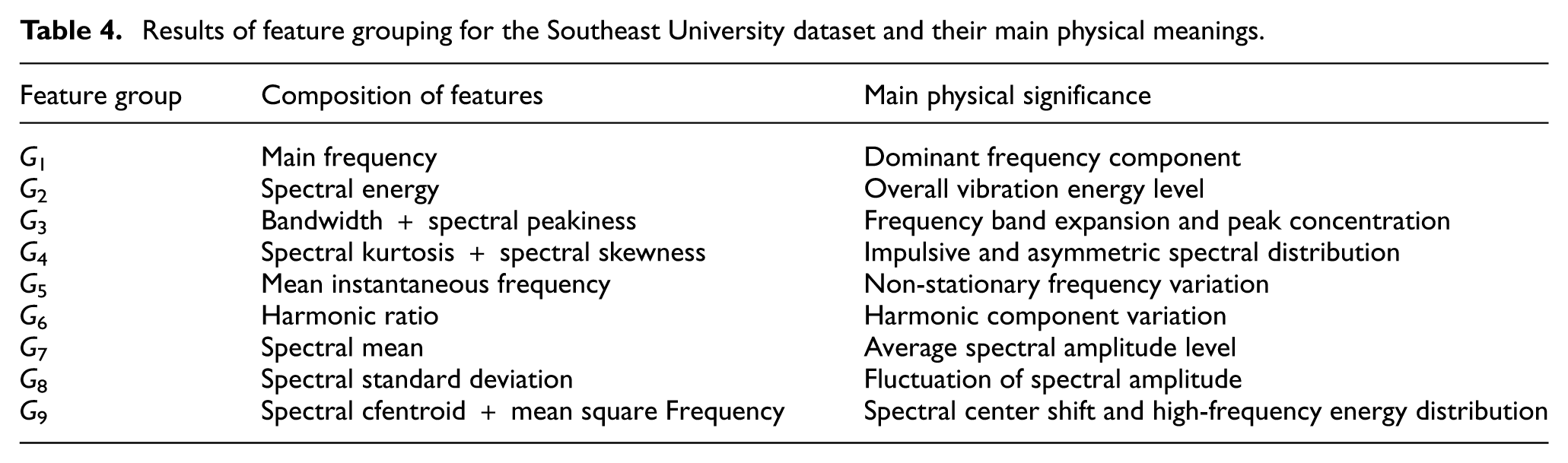
As shown in Table 4, compared with the eight feature structures identified in the field measurement data, the Southeast University dataset comprises nine feature structures. These results demonstrate that the method described in this paper does not rely on a fixed, manually defined combination of features, but rather automatically adjusts the grouping results based on the correlations among frequency-domain features across different datasets. Energy-related statistical features in the construction site data tend to exhibit stronger correlation, whereas some energy and amplitude statistical features in the Southeast University data remain independent, reflecting differences between the two datasets in terms of signal fluctuation and spectral distribution characteristics. The distribution of 3D structures under different clustering methods is shown in Figure 8.
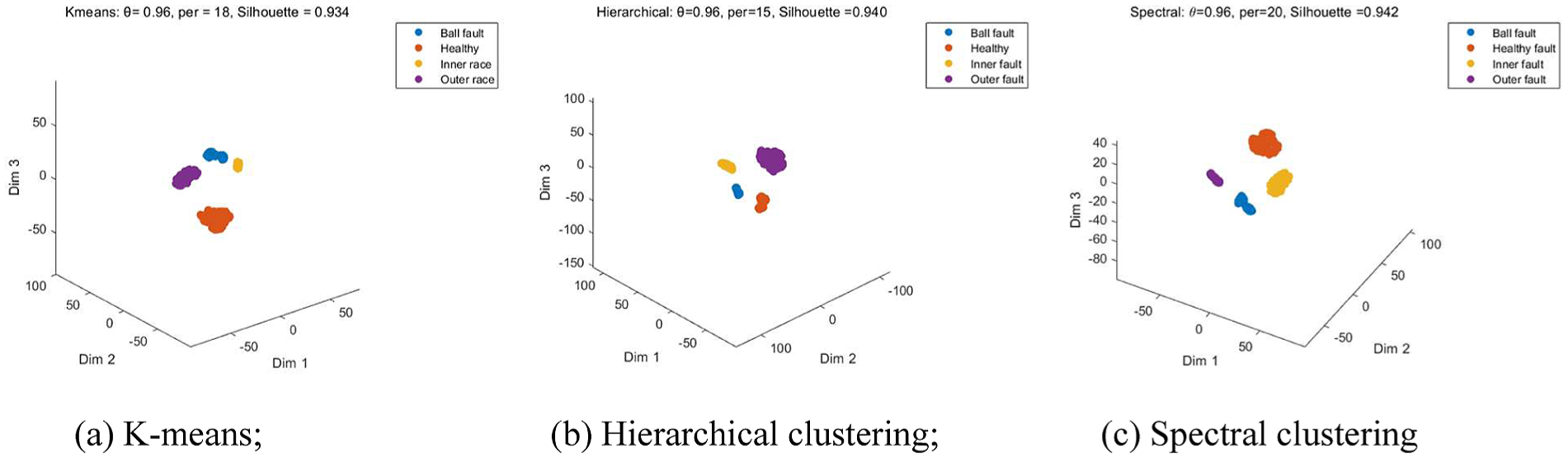
Distribution of 3D structures in the Southeast University dataset under different clustering methods: (a) K-means, (b) hierarchical clustering, and (c) spectral clustering. 3D: three-dimensional.
As shown in Figure 8, the four sample categories all form distinct clusters in 3D space. The distribution of samples in the “Healthy” class is relatively compact and clearly separated from the three failure states; there was also no significant overlap between the Ball fault, the Inner fault, and the Outer fault. Compared to field measurement data, the cluster patterns in the Southeast University dataset are more concentrated, which is attributed to the relatively stable collection environment and minimal variations in operating conditions. Under the optimal parameter conditions for each clustering method, the kurtosis values for K-means, hierarchical clustering, and spectral clustering were 0.934, 0.940, and 0.942, respectively. The results from these three methods were similar, indicating that this 3D structure maintains a relatively stable distribution pattern under different clustering criteria.
Overall, the validation results using the Southeast University dataset indicate that the method proposed in this paper can still produce a relatively clear 3D structural distribution across different data sources, fault types, and sample sizes. The number of feature groups was adjusted from eight groups based on field measurement data to nine groups based on the Southeast University dataset, further demonstrating that the method can adapt to the frequency-domain correlation structure inherent in the data. This result validates the stability and applicability of the method proposed in this paper across different datasets.
Conclusion
To address the challenges of weak spectral differences, ambiguous sample boundaries, and the difficulty in directly distinguishing fault conditions in gearbox system vibration signals under complex operating conditions, this paper proposes a 3D structural analysis method based on frequency-domain statistical features to perform structural identification and distribution analysis on vibration data under different operating conditions. Experimental analysis of field measurement data and the publicly available dataset from Southeast University reveals that different fault states form structurally stable, well-defined sample distributions in 3D feature space. Field measurement data show that the profile coefficient reaches 0.935 under optimal parameter conditions, which is significantly better than the results obtained from the original frequency-domain characteristics and the traditional Fisher weighting method; the public dataset maintains a high silhouette coefficient across different clustering methods, indicating that this method effectively enhances the spatial separability between different operational states. Further comparative analysis was conducted using K-means, hierarchical clustering, and spectral clustering. The morphological patterns of the sample space remained consistent across different clustering methods, indicating that the resulting structure is not dependent on a single clustering algorithm and exhibits good stability and applicability. The resulting feature set exhibits a certain correlation with fault vibration characteristics such as changes in the dominant frequency, energy fluctuations, bandwidth expansion, impact spikes, harmonic components, and shifts in the center of gravity; this indicates that the 3D structure developed in this paper not only achieves effective separation in the sample space but also provides an explanation based on changes in frequency-domain features and the mechanisms of mechanical vibration. From an engineering perspective, by analyzing the distribution of 3D structures, it is possible to help identify clusters of anomalous samples and trace potential sources of failure, thereby providing a basis for analyzing failure mechanisms and identifying potential failure locations. When abnormal structures that deviate significantly from the normal state appear in 3D space, targeted inspections of key components can be conducted in conjunction with corresponding changes in characteristics, providing a basis for equipment inspections, adjustments to maintenance schedules, and preventive maintenance. Furthermore, the feature structure developed in this paper can not only be used for fault state analysis under complex operating conditions but also serve as effective input for subsequent intelligent diagnostic models, providing a more stable, distinguishable, and physically meaningful feature foundation for fault identification and condition prediction.
Footnotes
Author contributions
Funding
The authors disclosed receipt of the following financial support for the research, authorship, and/or publication of this article: This research was supported by the National Natural Science Foundation of China (grant no. 62363018), the China General Nuclear Power Group Chuxiong Dayao Wind Power Co., Ltd (grant no. 020-XN10-B-2024-C45-P.N.99-00015), and the Discipline Development Project of the School of Civil Aviation and Aeronautics, Kunming University of Science and Technology.
Declaration of conflicting interests
The authors declared no potential conflicts of interest with respect to the research, authorship, and/or publication of this article.
Data availability statement
The data cannot be made publicly available upon publication because the cost of preparing, depositing and hosting the data would be prohibitive within the terms of this research project. The data that support the findings of this study are available upon reasonable request from the authors.