Residual wall thickness profile measurement of thin plates based on phased array zero-group-velocity mode

Abstract

Plate-like structures in harsh environments often experience wall thickness loss, making accurate residual thickness assessment critical for timely maintenance and failure prevention. This article presents a phased-array zero-group-velocity (PA-ZGV) method for profiling the residual thickness of thin plates by combining the material-property sensitivity of zero-group-velocity (ZGV) Lamb modes with the wave-steering capabilities of phased arrays (PAs). Two key enhancements were introduced: (1) optimized phased-array excitation to amplify the intensity of the S1-ZGV mode, and (2) time-domain summation (TDS) processing to eliminate time-truncation limitations. As a result, four ZGV-based methods for thickness profile reconstruction were developed and validated through finite element simulations. Experimental validation using a linear PA transducer on aluminum plates with grooved defects demonstrated excellent agreement with high-frequency pulse-echo and line-laser scanning methods, achieving an average root-mean-square error below 0.03 mm. All four ZGV-based methods achieve high accuracy in central-region measurements. Under reflection-prone edge-region conditions, however, the PA-assisted and TDS-assisted strategies, particularly PA-ZGV-TDS, provided more robust ZGV frequency extraction and lower reconstruction errors than the conventional single-element ZGV method. These findings establish PA-assisted ZGV approaches as a low-frequency, high-precision, and robust solution for residual thickness mapping in industrial thin-walled structures.

Keywords

lamb wave zero-group-velocity mode phased array time-domain summation residual wall thickness profile

Introduction

The application of thin-walled structures has expanded across various industries, including aerospace, wind power, and shipbuilding.^1,2 Over time, these structures can develop subtle defects, such as wall thickness loss due to surface wear or corrosion. These defects may degrade the mechanical properties and potentially lead to severe engineering failures. Therefore, periodical detection or online monitoring of residual thickness of thin-walled structures is critical. Current wall thickness measurement methods include conventional mechanical gauges (e.g., micrometer calipers), optical technique,^3,4 eddy current testing,^5,6 and X-ray.^7,8 While these conventional approaches remain prevalent, their practical implementations are constrained in some aspects. Mechanical gauges risk inducing surface deformation and demonstrate reduced efficacy in geometrically complex components; optical methods require surfaces with optimal reflectivity; eddy current techniques are restricted to conductive materials; and X-ray necessitates significant infrastructure while posing radiation exposure.

Ultrasonic testing offers various advantages,^9–11 such as nondestructive evaluation, portable devices, and high accuracy. Currently, the ultrasonic thickness measurement includes pulse-echo (PE) method, acoustic resonance (AR) method, and guided wave (GW) method. The PE method obtains thickness by measuring the time-of-flight (ToF) of adjacent echoes with the known sound velocity. Maev et al.¹² employed a broadband focused immersion transducer to measure the thickness of multilayered curved polymers (0.130–2.033 mm), achieving a minimum error of 0.6%. Kruger et al.¹³ utilized the PE method to measure thicknesses up to 100 mm at high temperatures up to 1250°C. Zhang et al.¹⁴ proposed a dual-wave correction method to simultaneously monitor steel plate thickness changes and temperature variations. Wang et al.¹⁵ developed a thickness measurement method for highly attenuating materials with quasi-static component (QSC) pulses induced by high-frequency longitudinal wave tone bursts in elastically nonlinear solids. They determined thickness by precisely measuring the ToF between two consecutive QSC pulse echoes.¹⁵ However, these PE methods rely on high-frequency ultrasound with a very short wavelength for thin plates. Meanwhile, the AR method works well when the material thickness is an integer of half-wavelength ( $λ / 2$ ), where reflected and incident waves interfere to form standing waves. The thickness is determined by adjacent resonance frequencies. Dixon et al.¹⁶ utilized shear wave resonance to measure the thickness of an 11 µm polymer coating on an aluminum substrate. Zhang et al.¹⁷ applied the spacing of parallel resonance frequencies to evaluate thickness variations in elastic plates, and the relative error for the thickness ranging from 0.1 μm to 1 mm is less than 5%. Despite widespread application and high accuracy for wall thickness measurement, PE and AR methods are limited to measuring thickness only at the point directly beneath the transducer.

Ultrasonic GW methods are preferred for quickly inspecting large areas or when accessibility to the structure is limited.^18,19 Several studies have developed GW methods based on Lamb modes or shear horizontal modes to quantify the residual wall thickness. Satyarnarayan et al.²⁰ utilized a piezoelectric transducer mounted on an angled wedge to generate a higher-order Lamb wave for axial stress corrosion cracks in pipe support regions. However, this technique relies on the amplitude-based features, leading to challenges in the reliable quantification, because the amplitude is often affected by factors such as the coupling state and external prestress. Recently, frequency-based methods based on the higher-order GW modes have attracted attentions in quantitative wall thickness measurement. Tzaferis et al.²¹ conducted a study on wall loss quantification using the cut-off frequency of SH1 mode excited by a phased array (PA) technique. Suresh et al.²² developed a broadband excitation method with linear arrays to extract the cutoff characteristics of Lamb wave A1 mode, enabling residual thickness quantification in thin-walled structures with a maximum error of 2.3%. Heinlein et al. utilized SH1 mode’s cut-off frequency for thickness measurement with uneven surfaces. The standard deviation of the thickness measurements was less than 0.05 mm.²³ Although existing research has explored higher-order GW methods with arrayed transducers for wall thickness loss, these approaches are limited to determining maximum loss and lack the capability for full residual thickness profile reconstruction.

Meanwhile, a series of special GW modes, known as zero-group-velocity (ZGV) modes, have been investigated since the 1950s, when Tolstoy et al. first demonstrated their existence and resonance properties.²⁴ Its nature of zero group velocity causes acoustic energy trapped around the excitation region,^25,26 making it highly sensitive to local variation in thickness,^27,28 material properties,²⁹ and defects.³⁰ Compared to conventional GW methods, aiming for long-distance and wide-range measurements, the ZGV method enables precise local measurements. Matsuo et al.³¹ applied the ZGV Lamb waves method to measure the thickness of multilayered structures and assessed their bonding quality. Pan et al.³² proposed a multimodal ZGV method based on laser ultrasound to measure the layer thicknesses in a thin bilayer. Li et al.³³ investigated the combined ZGV harmonics generated by guided-wave mixing and applied to evaluate local material degradation. Yuan et al.³⁴ extracted the ZGV feature in the carbon fiber-reinforced plastic (CFRP)—Nomex honeycomb structure to detect and locate debonding defects with a diameter of 20 mm. The above studies demonstrate that the ZGV modes are highly sensitive to local material variation. Furthermore, since the ZGV method is based on frequency-domain features, its accuracy is unaffected by time resolution. These inherent merits position the ZGV-based method as an attractive solution, simultaneously replacing conventional high-frequency PE method and enabling profile reconstruction across thin-walled structures.

Laser ultrasound is currently the dominant technology for excitation and reception of ZGV Lamb waves.³⁵ However, the disadvantages, such as large size, high cost, and low signal-to-noise ratio (SNR) make it unsuitable for field test. Recently some studies have focused on developing efficient and flexible methods to excite ZGV Lamb waves. Meng et al.³⁶ successfully excited ZGV feature guided waves in welded joint with air-coupled transducers. He et al.³⁷ designed a compact wedge transducer to excite the S1-ZGV Lamb waves in aluminum plates, and explored optimal excitation conditions for localized stress measurements. Guo et al.³⁵ utilized a polyvinylidene fluoride (PVDF) comb transducer to excite the ZGV modes by carefully designing the comb electrodes. They efficiently excited the ZGV Lamb waves in laminates and assessed surface corrosion damage by analyzing the amplitude of its resonance peaks. However, current methods to excite ZGV Lamb waves have certain limitations. The air-coupled ultrasonic transducer suffers from large acoustic impedance mismatch and low-energy transfer efficiency. The wedge transducer needs to determine the exact incident angle and the proper receiving distance. The comb transducer requires deliberated design of the comb electrode with the known ZGV wavelength.

On the other hand, PA ultrasonic testing enables wave steering and focusing to scan the investigated region. Recently, it has been proposed to conveniently control the longitudinal critically refracted wave through time delay optimization, replacing the conventional wedge transducer.³⁸ Besides, PA has been widely applied to control the excitation and propagation of desired GW modes, including some high-order GW modes.^21–23 Building upon these fundamental insights, an advanced ZGV technique, termed phased array zero-group-velocity (PA-ZGV), is proposed here. The PA-ZGV methodology aims to overcome four challenges of conventional ZGV implementations: (1) enhanced ZGV mode excitation and reception, (2) capability to reconstruct thickness profile, (3) field-deployable ZGV measurement system.

The subsequent sections of this article are arranged as follows. Methodology for ZGV-based thickness profiling provides theoretical background for ZGV-based thickness profiling measurement enhanced by PA excitation. Finite element simulations validate the method’s capability to quantify thickness variations via S1-ZGV using linear PAs. Experimental validation details experiment studies, including the S1-ZGV mode excitation and reception with optimized parameters, thickness profile reconstruction, and accuracy quantification validated against 3D line-laser scanning and high-frequency PE methods. Concluding remarks are presented in Conclusion.

Methodology for ZGV-based thickness profiling

TDS-based ZGV frequency extraction

Lamb waves are dispersive, meaning that their velocities depend on the excitation frequency. The relationship between velocity and frequency is described by the well-known Rayleigh–Lamb equation³⁹:

\frac{\tan (qh)}{\tan (ph)} + \frac{4 k^{2} pq}{(q^{2} - k^{2})^{2}} = 0 for symmetric modes,

(1)

\frac{\tan (qh)}{\tan (ph)} + \frac{(q^{2} - k^{2})^{2}}{4 k^{2} pq} = 0 for antisymmetric modes,

(2)

where $k$ denotes the wavenumber and $h$ is the half-thickness of the plate. $p^{2} + k^{2} = {(\frac{ω^{2}}{C_{L}})}^{2}$ , $q^{2} + k^{2} = {(\frac{ω^{2}}{C_{S}})}^{2}$ , where $ω$ is the angular frequency, while $C_{L}$ and $C_{S}$ are the longitudinal and shear wave velocities, respectively. By substituting $C_{L}$ = 6370 m/s, $C_{S}$ = 3189 m/s, and $h$ = 0.75 mm into the above equations, the dispersion curves of a 6061-aluminum plate with a thickness of 1.5 mm are obtained. This study focuses on the S1-ZGV mode, which arises from the interaction between the forward-propagating S1 mode and the backward-propagating S2 mode.³⁷ Its energy is highly localized near the excitation region, that is, the group velocity vanishes as⁴⁰:

C_{g} = \frac{d ω}{d k} = 0,

(3)

corresponding to a zero slope on the frequency-wavenumber curve.⁴¹ In this case, the frequency of the S1-ZGV mode is determined to be 1.918 MHz.

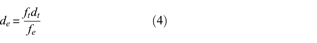
For a given material, the frequency-thickness product of the S1-ZGV mode remains constant, thus, any variation in plate thickness results in a corresponding frequency shift. Specifically, an increase in thickness leads to a shift of the S1-ZGV frequency toward lower values, as illustrated in Figure 1(a). The quantitative relationship between the S1-ZGV frequency and thickness is shown in Figure 1(b). Consequently, once the theoretical frequency-thickness product is known, the thickness $d_{e}$ can be inversely determined from the measured resonant frequency $f_{e}$ ⁴²:

d_{e} = \frac{f_{t} d_{t}}{f_{e}}

(4)

Here, $f_{t} d_{t}$ denotes the theoretical frequency-thickness product of the S1-ZGV mode, which is 2.877 MHz mm for the 1.5-mm-thick aluminum plate used in this study.

Figure 1.

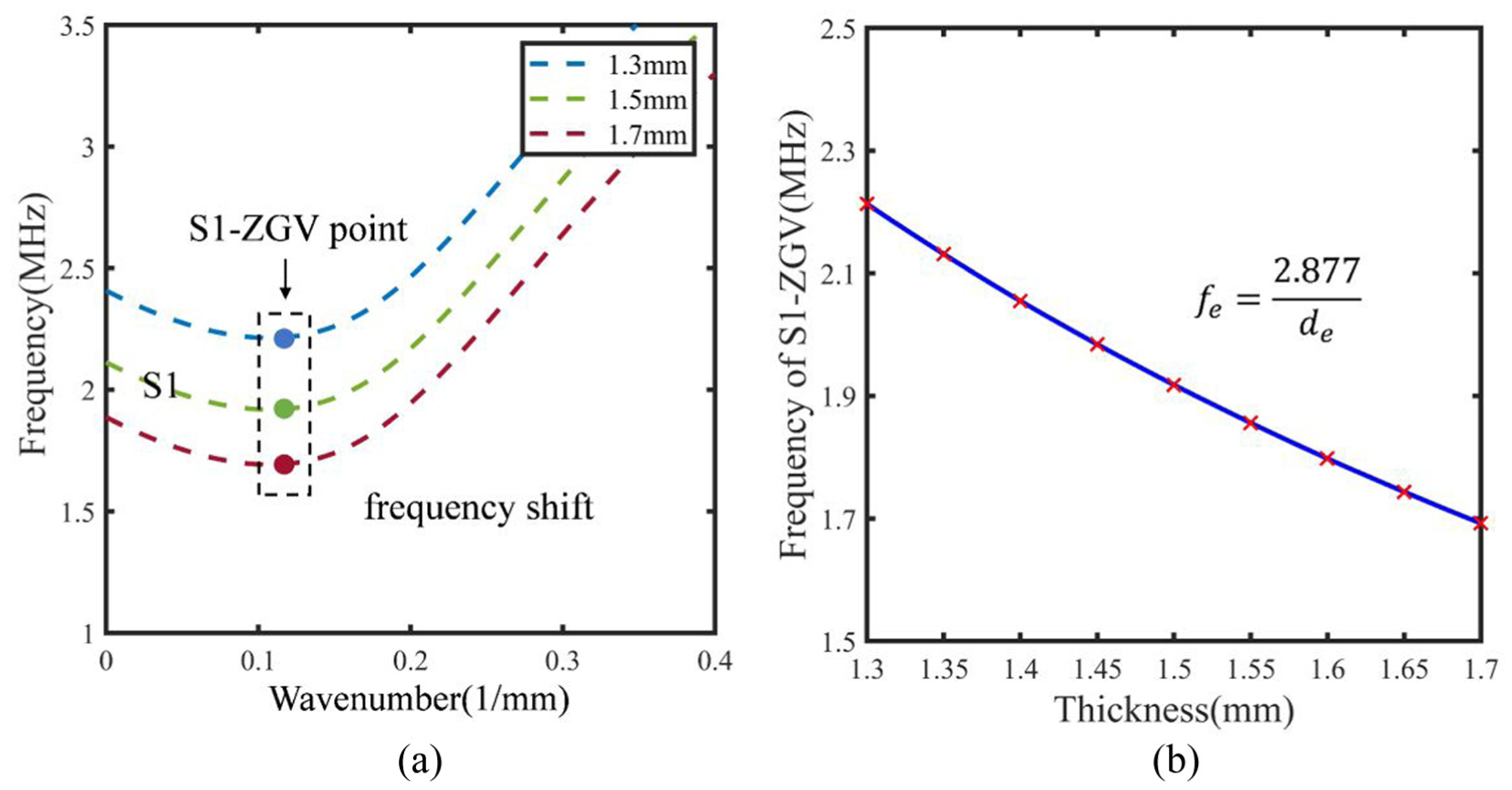
Dispersion curve of a 1.5 mm 6061 aluminum plate: (a) frequency shift of S1-ZGV mode and (b) the function of thickness.

Thus, the thickness profile can be reconstructed using an array transducer, which is referred to here as the conventional ZGV method. As shown in Figure 2(a), a pulse–echo configuration is employed, in which each element of the linear array sequentially acts as both transmitter and receiver to excite and capture the S1-ZGV response. The resonance portion of the received signal is truncated in the time domain and then processed by Fast Fourier Transform (FFT) to extract the S1-ZGV frequency. The local thickness at each element position is subsequently estimated using Equation (4). This procedure is repeated across all array elements to reconstruct the thickness profile over the array coverage area.

Figure 2.

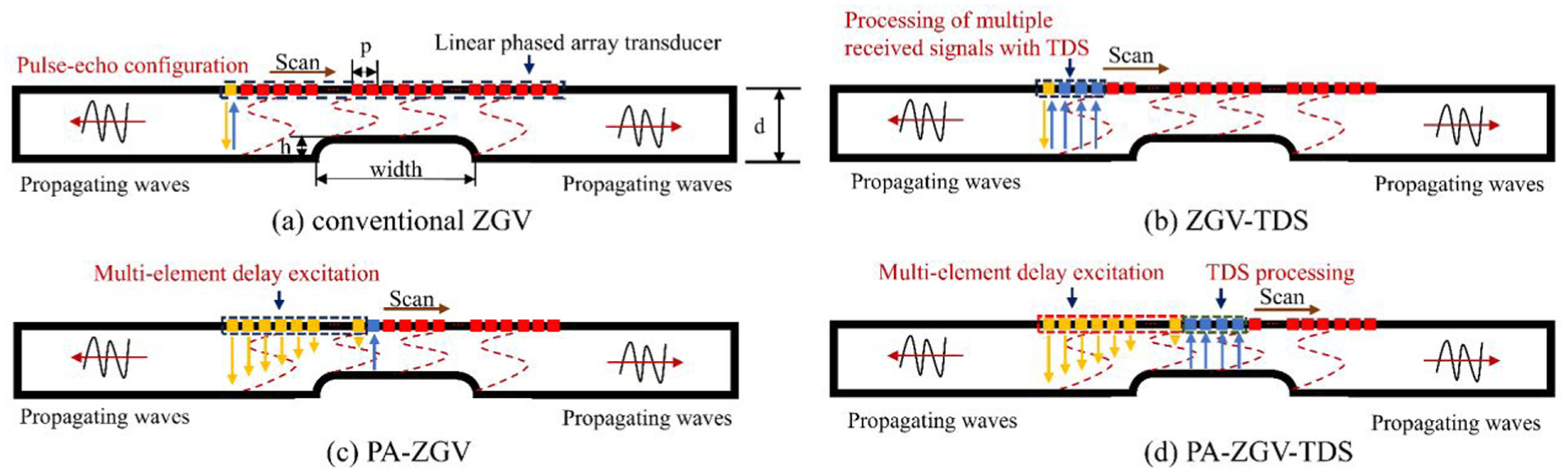
ZGV-based methods for thickness profiling. (a) conventional ZGV, (b) ZGV-TDS (c) PA-ZGV and (d) PA-ZGV-TDS.

However, conventional ZGV method relies on time-domain truncation of the resonance signal, and the extracted spectrum can become unstable in the presence of direct waves or reflection-induced interference. To improve the robustness of resonance-frequency extraction, a time-domain summation (TDS) strategy is introduced, referred to as the ZGV-TDS method, as shown in Figure 2(b). This method enhances S1-ZGV resonance and improves measurement accuracy by coherently summing signals from receivers at different propagation distances.⁴³ This strategy leverages the extended lateral influence region of the S1-ZGV mode, while exploiting the distance-dependent phase variation of propagating modes. As a result, TDS simultaneously amplifies the resonance peaks and suppresses unwanted propagation wave components.

The summed signal $y_{n} (t)$ from $n$ array elements is given by:

y_{n} (t) = \sum_{i = 1}^{n} x_{i} (t)

(5)

The resulting signal $y_{n} (t)$ is then transformed into the frequency domain via FFT to obtain $Y (f)$ , followed by normalization to yield $Y_{norm} (f)$ as such:

Y_{norm} (f) = \frac{Y (f)}{\max (Y (f))}

(6)

The S1-ZGV resonance frequency is identified as the dominant peak in $Y_{norm} (f)$ . The ZGV-TDS approach improves frequency extraction through strategically signal combination from multiple array elements within a predefined spatial range.⁴⁴ This method offers two main advantages: (1) elimination of time-domain truncation of the resonance signal, and (2) improved accuracy and robustness of frequency estimation without case-specific parameter tuning.

Phased array enhanced ZGV excitation

Although ZGV-TDS method improves thickness profiling through frequency extraction, it still relies on single-element excitation, which limits both the amplitude and spectral purity of the generated S1-ZGV mode. To overcome this limitation, PA control is further introduced to selectively enhance the target ZGV response.

Common methods for Lamb-wave excitation include angular excitation and multielement excitation. Angular excitation is widely used in air-coupled and wedge-based transducers based on Snell’s law, whereas comb transducers represent a typical multielement approach for exciting specific wavelengths. More recently, Veit et al.⁴⁵ employed a phased-array transducer with controlled bandwidth and beam angle to selectively excite a single Lamb mode in a narrow region with high frequency-thickness products. Verma et al.^46,47 further extended this concept to Rayleigh wave, achieving enhanced SNR and beam directivity. Building on these developments, a phased-array strategy is adopted here to enhance the excitation of S1-ZGV mode.

For a linear phased-array transducer as shown in Figure 3(a), the amplitude of the S1-ZGV mode is maximized when the condition $e / λ \pm t_{0} f = m$ is satisfied, where $e$ is the element pitch, $λ$ is the wavelength, $t_{0}$ is the time-delay gradient, and $m$ is an arbitrary integer. When the pitch is much smaller than the wavelength, $m$ approaches 0. In this study, the element pitch is significantly smaller than the S1-ZGV wavelength ( $λ_{ZGV}$ =5.66 mm), leading to a simplified phase-matching condition as

C_{ph, ZGV} = λ_{ZGV} \cdot f = \frac{e}{t_{0}}

(7)

where $C_{ph, ZGV}$ = 10.86 km/s is the phase velocity of the S1-ZGV mode. To enhance the excitation of the S1-ZGV mode, the time delay applied to the ith element $t_{i}$ is defined as follows:

t_{i} = (i - 1) t_{0}, t_{0} = \frac{e}{C_{ph, ZGV}}

(8)

Figure 3.

(a) Schematic diagram of linear PA transducer for S1-ZGV excitation and (b) the time delay for the first 20 exciting elements.

The calculated time delays for the first 20 elements are presented in Figure 3(b). Through constructive interference among array elements, the S1-ZGV mode is reinforced while other modes are effectively suppressed.

Based on the PA-enhanced excitation scheme, two implementations are developed for thickness profiling. The first, referred to as PA-ZGV, enhances the excitation of the S1-ZGV mode while retaining single-element reception for frequency extraction. The second, referred to as PA-ZGV-TDS, combines PA-enhanced excitation with the TDS-based reception strategy. As shown in Figure 2(c), the PA-ZGV method employs a phased-array subaperture to selectively enhance the S1-ZGV mode via constructive interference. A neighboring element is used for signal reception, and the local thickness is estimated using Equation (4). The thickness profile is reconstructed through spatial scanning, following the same procedure as in the conventional ZGV method. As shown in Figure 2(d), the PA-ZGV-TDS method integrates PA-enhanced excitation with TDS-based reception. The subaperture improves the excitation efficiency of the S1-ZGV mode, while signals from multiple adjacent elements are coherently summed prior to frequency extraction. The local thickness is then calculated using Equation (4), and the final thickness distribution is obtained via spatial scanning.

Finite element simulations

Effect of coupling on ZGV frequency

This section examines the influence mechanism of the coupling agent layer on the ZGV mode frequency. A fully coupled, transient two-dimension finite-element (FE) model was established on the COMSOL Multiphysics, integrating electromechanical conversion, acoustic-wave propagation, and acoustic-structure interaction. The model aims to replicate the pitch-catch operation of a single piezoelectric transducer element through a multilayer medium (piezoelectric crystal—coupling layer—test plate), and reception. Along the wave-propagation direction, the model comprises three physical domains: the piezoelectric crystal domain, the coupling-layer domain, and an infinite solid-plate domain. The two-dimensional model schematic is shown in Figure 4(a).

Figure 4.

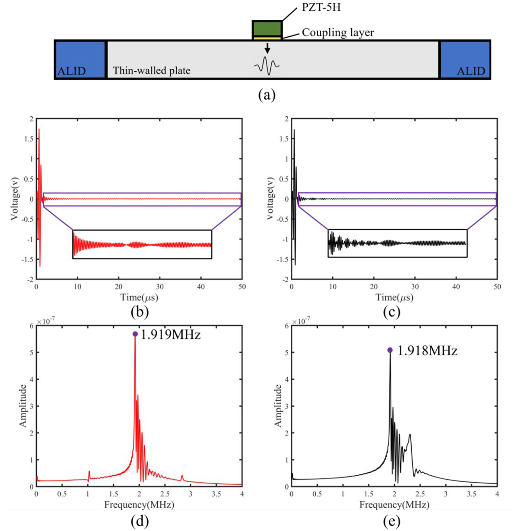
(a) A two-dimension FE model with and the corresponding waveform and spectra for different coupling-layer thickness: (b) and (d) for 0.001 mm, and (c) and (e) for 0.01 mm.

The material properties are assigned as follows: PZT-5H for the piezoelectric crystal; a Newtonian fluid with a density of 1100 kg/m³ and a longitudinal-wave velocity of 1700 m·s⁻¹ (representative of typical water-based industrial gels) for the coupling layer; and Al6061 with a density $ρ$ = 2704 kg/m³, Young’s modulus $E$ = 72 GPa, and Poisson’s ratio $υ$ = 0.331 for the plate. The piezoelectric crystal has dimensions of 0.5 mm (length) × 1 mm (height). Two coupling-layer thicknesses, 0.01 mm and 0.001 mm, were used. The plate was modeled with a length of 100 mm and a thickness of 1.5 mm. To approximate an infinite plate and eliminate boundary reflections, the absorbing layers with increasing damping (ALID) were applied at both ends of the solid domain. A three-cycle Hann-windowed sinusoidal signal centered at 2 MHz, matching the experimental pulse bandwidth, was applied as the excitation. The resulting frequency-thickness product of 3 MHz mm closely approached the theoretical S1-ZGV value of 2.877 MHz mm.

The time-domain signals received by the PZT-5H element were first extracted for coupling-layer thicknesses of 0.01 and 0.001 mm. These signals were then processed using FFT within a time window from 1.5 to 50 μs to reduce the influence of the direct excitation signal on the spectral content. Zero-padding and windowing were applied during the FFT to improve spectral resolution. As shown in Figure 4, the resulting spectrum displays a sharp resonance peak. For the 0.001 mm coupling layer, the resonance peak occurs at 1.919 MHz; for the 0.01 mm layer, it appears at 1.918 MHz. Both values align closely with the theoretical S1-ZGV frequency of 1.918 MHz, confirming that this peak corresponds to the ZGV mode. Furthermore, varying the coupling-layer thickness has only a minor effect on the ZGV frequency: a 10-fold increase in thickness shifts the frequency by merely about 1 kHz, which remains within an acceptable margin of error for ZGV-based measurements. Several smaller-amplitude high-frequency peaks are also visible to the right of the main ZGV peak. These are likely attributable to higher-order plate-wave modes, inherent resonances of the piezoelectric crystal, or resonances within the coupling layer itself. Since these secondary peaks do not interfere with the identification and extraction of the ZGV mode, they are not analyzed further in this study.

Physically, this weak frequency shift can be attributed to the fact that the S1-ZGV resonance is governed primarily by the plate’s local dispersion relation, that is, it is mainly determined by the plate thickness and bulk elastic properties. In the present configuration, the couplant layer is much thinner and possesses a significantly lower acoustic impedance. Previous studies on ZGV resonances in layered systems have shown that the resonance-frequency shift induced by an additional surface layer is approximately proportional to its mass loading.⁴⁸ In the present case, however, the couplant is a fluid-like medium rather than a solid bonded layer, and the effective loaded region beneath each transducer element is spatially localized rather than continuous. As a result, its mass-loading effect is expected to be substantially weaker than that of a deposited metallic layer. Furthermore, because the fluid-like couplant does not sustain shear traction, its loading effect acts primarily as a weak normal perturbation, rather than a strong mechanical constraint on the ZGV standing-wave field.⁴⁹ Therefore, the couplant mainly affects the transmission efficiency and attenuation, leading to variations in signal amplitude and spectral SNR, whereas its perturbation to the intrinsic resonance frequency remains negligible.

S1-ZGV mode identification and enhancement

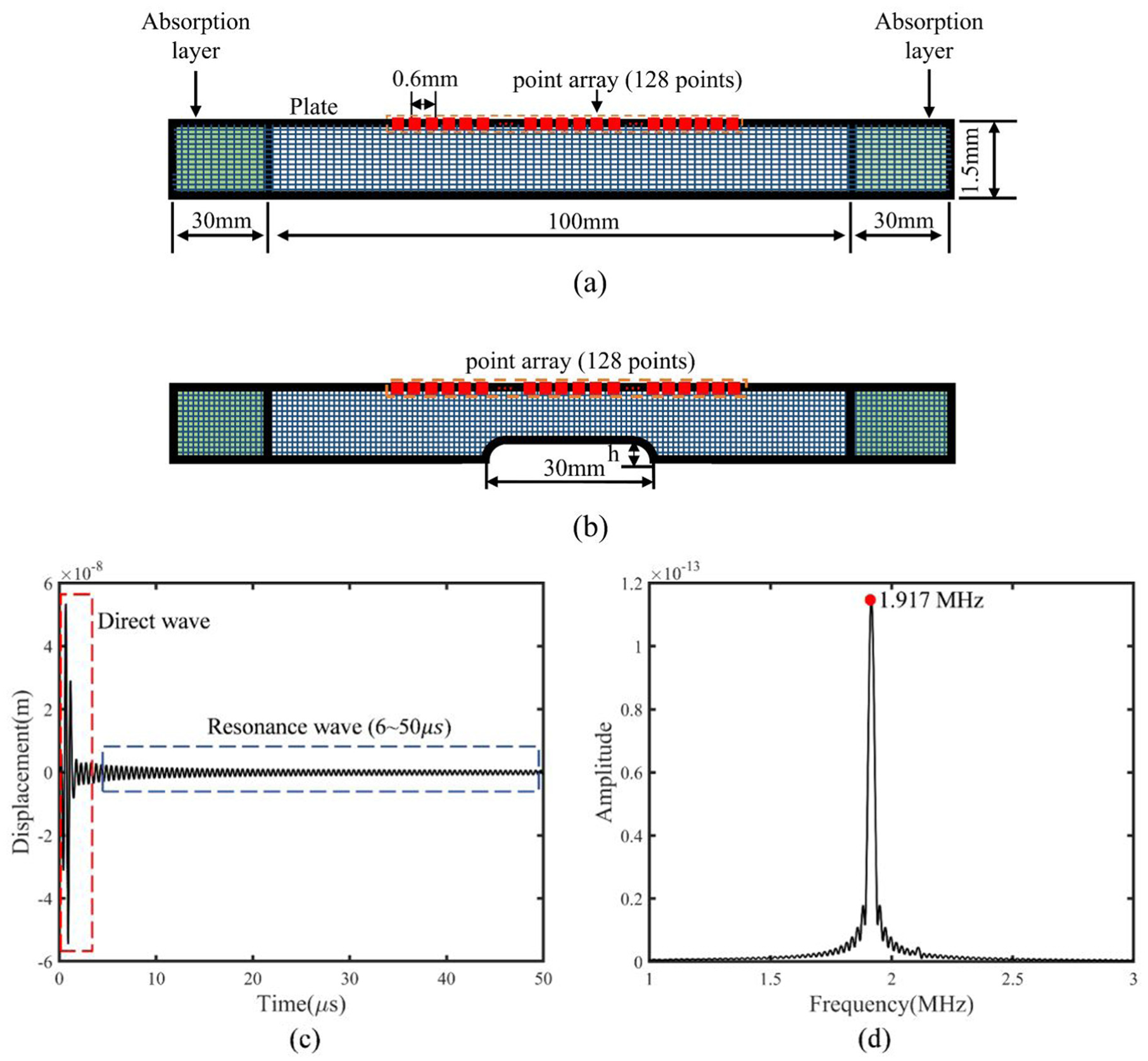
Considering the little influence and substantial computational cost associated with multiphysics modeling of piezoelectric crystals and coupling layers, subsequent simulations employed a simplified point-source model. The simulated Al6061 plate ( $ρ$ = 2704 kg/m³, $E$ = 72 GPa, $υ$ = 0.331) featured a 100 mm length and uniform 1.5 mm thickness. Boundary reflections were minimized using absorption layers at both ends. A 128-element linear array with a pitch of 0.6 mm matching subsequent experiment setup was implemented. The intact plate and thickness-loss plate are shown in Figure 5(a) and (b). The thickness loss plates were set as a 30-mm-long defects with depths of 0.1, 0.15, and 0.2 mm, featuring rounded edges to minimize scattering and mode conversion.

Figure 5.

2D finite element models for (a) intact plate and (b) thickness-loss plate along with (c) typical received A-scan signal and (d) the spectra of resonance wave.

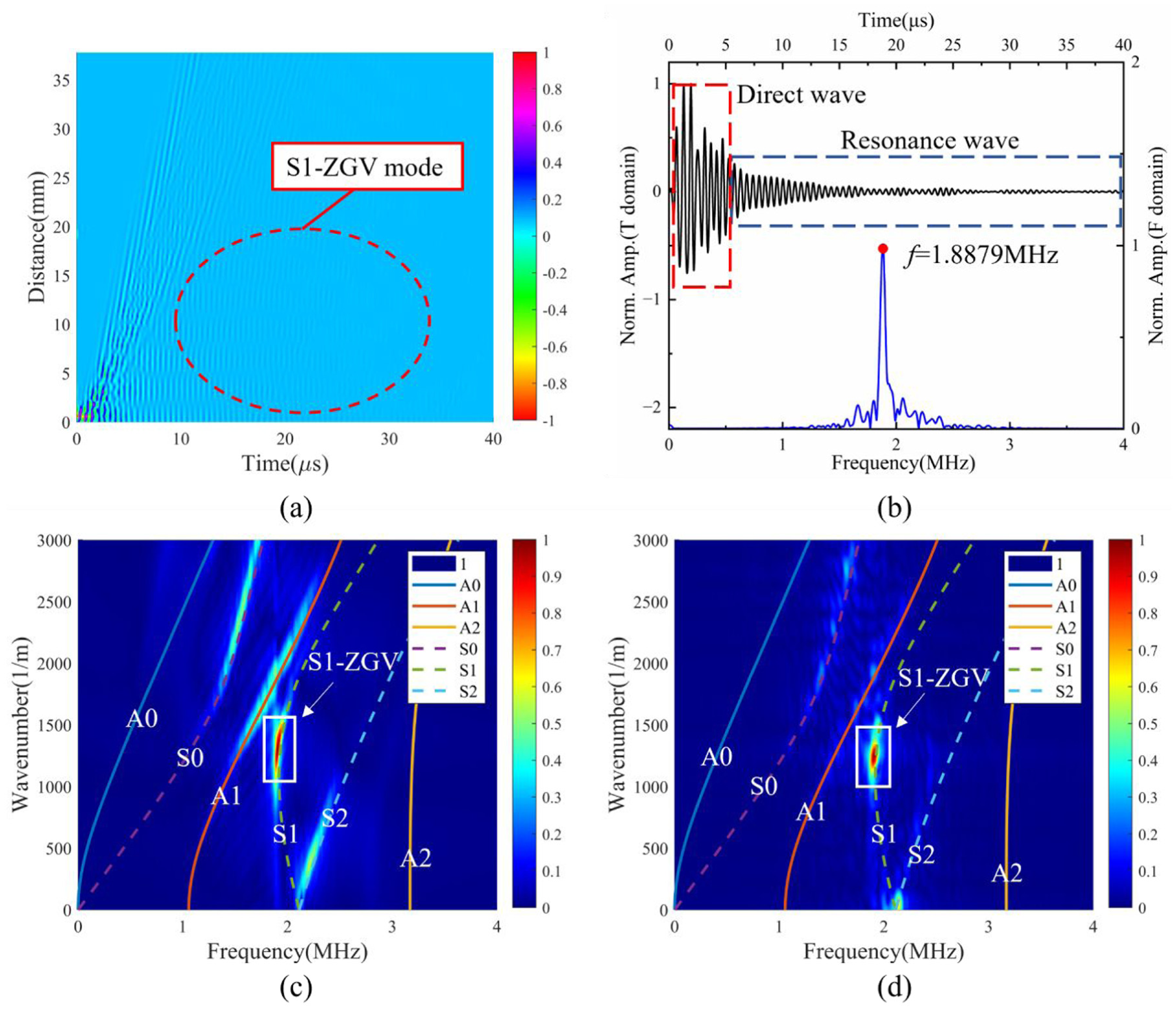
Figure 5(c) shows a typical pulse-echo waveform from the point source simulation, consisted of both the direct wave and resonance wave component. Figure 5(d) displays the corresponding amplitude spectrum of the resonance signal (6–50 $μ s$ ), processed with Hanning windowing and zero-padding. This spectrum reveals a sharp resonance peak at 1.917 MHz. Given the plate thickness of 1.5 mm and the theoretical S1-ZGV frequency-thickness product of 2.877 MHz mm, the expected resonance frequency is 1.918 MHz. The simulated center frequency (1.917 MHz) showed excellent agreement (0.05% deviation) with the theoretical prediction.

To characterize the S1-ZGV mode, normal displacement signals were acquired along a 38.4 mm with a pitch of 0.6 mm. The B-scan in Figure 6(a) displays several high-energy direct waves, followed by continuous low-amplitude resonance signals. Wavenumber-frequency analysis^50,51 of time-windowed signals (0–50 $μ s$ ) in Figure 6(b) identify dominant modes (A0, S0, A1, S1, S1-ZGV, and S2), exhibiting good agreement with theoretical dispersion curves. The prominent A0/S0 energy is attributed to the high excitability of fundamental modes, while higher-order S1 and S2 modes display lower amplitudes. Spatial FFT of resonant signals (Figure 6(c)) reveals the energy distribution of S1-ZGV mode, exhibiting periodic patterns centered at the excitation source. Measured spatial periodicity (2.912 mm) in Figure 6(d) aligns closely with the theoretical S1-ZGV half-wavelength: $\frac{λ}{2} = \frac{C_{ph, S 1 - ZGV}}{2 f} = 2.831 mm$ . This standing wave pattern results from counter-propagating waves with comparable amplitude. It can be observed that the resonance frequency slightly increases, while amplitude decays with the distance from the source. This occurs because that Lamb S1/S2 modes below $f_{S 1 - ZGV}$ are evanescent, whereas only propagating S1/S2 mode above $f_{ZGV}$ contribute to response at distances beyond $λ_{ZGV}$ from the source.⁵²

Figure 6.

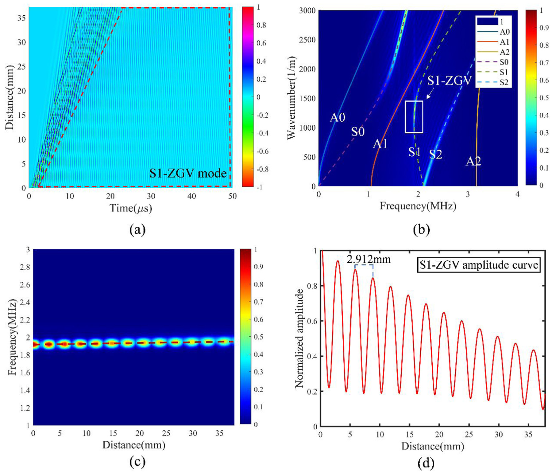
Wavefield in FE simulations: (a) B-scan signal (the resonance signal within the red box is the S1-ZGV mode), (b) wavenumber-frequency analysis, (c) spatial spectra (the red dashed line traces the peak amplitude), and (d) amplitude variation with distance.

Then, the TDS technique was numerically validated, with receiver elements constrained within a half-wavelength (2.831 mm) of the S1-ZGV mode. Considering the 0.6 mm pitch of the linear array, five spatially distributed signals were summed. Figure 7 compares temporal waveforms and amplitude spectra before and after TDS processing. Results demonstrate limited improvement under simulation conditions. The temporal waveforms show negligible modifications (Figure 7(a)). The spectral analysis indicates suppression of propagating wave components in both low-frequency (<1.9 MHz) and high-frequency (>2.25 MHz) ranges adjacent to the resonance, as illustrated in Figure 7(b). In contrast, spectral amplification observed at 2.05 ± 0.1 MHz confirms the activation of the S1 thickness resonance mode, whose frequency is higher than that of the S1-ZGV mode and likewise corresponds to a resonant wave component. It should be noted that the FFT in this case was performed without applying any time window; instead, the complete acquired time-domain signal was transformed directly. Under this processing condition, the spectrum of a single array element exhibited a resonance frequency of 1.9150 MHz, which differs by 2 kHz from the frequency obtained in Figure 5(d)—a discrepancy attributable to the absence of time windowing. Following the application of TDS processing, the resonance frequency shifted from 1.9150 to 1.9153 MHz, thereby aligning more closely with the baseline reference signal (1.917 MHz). Based on these observations, employing the TDS method to enhance the unwindowed FFT results in only a marginal improvement for ideal-flat plates with well-designed absorbing boundary condition.

Figure 7.

Comparison of before and after TDS process: (a) A-scan signal, and (b) spectra.

For the S1-ZGV mode at 1.918 MHz ( $C_{ph, ZGV} = 10, 860 m / s$ ), a delay gradient of $t_{0}$ = 55.25 ns is yielded using Equation (8). The excitation length was set as one ZGV wavelength, with 10 elements activated based on array pitch. Normal displacements at 64 points downstream were recorded (Figure 8(a)) and wavenumber-frequency analysis with a 0–50 μs time window (Figure 8(b)). Compared to conventional ZGV excitation (Figure 6(a) and (b)), B-scan results show a prolonged resonance duration. Wavenumber-frequency result reveals significant suppression of A0, S0, A1, and S2 modes, along with 79.6% increase in S1-ZGV amplitude. The time-domain signal (Figure 8(c)) with a 6–50 μs window demonstrates enhanced resonance quality. Spectral analysis reveals a slight resonance frequency shift from 1.917 to 1.918 MHz, accompanied by an over four-time amplitude increase from 1.1535 $\times$ 10⁻¹³ to 5.4582 $\times$ 10⁻¹³. This analysis confirms that the PA-ZGV method achieves a superior spectral purity in S1-ZGV mode with resonance frequency converging to theoretical prediction.

Figure 8.

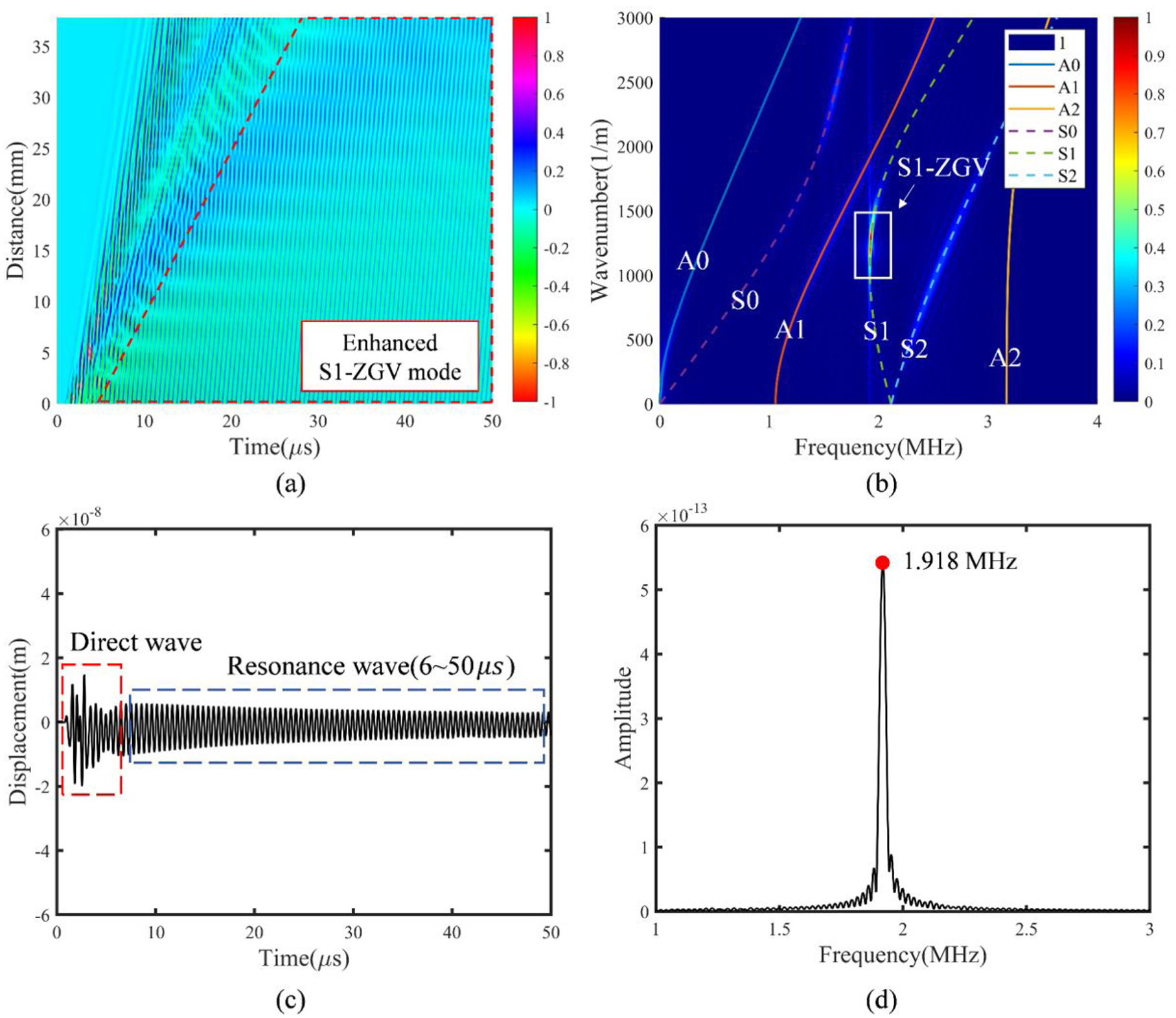
The wavefield of PA-ZGV in FE simulations: (a) B-scan wavefield, (b) wavenumber-frequency analysis from 0–50 μs, (c) received A-scan signal for a point adjacent to the excitation, and (d) the spectra of resonance wave.

Residual thickness profile reconstruction

Building on these findings, the feasibility for measuring wall thickness loss using the proposed methods was evaluated. First, the residual thickness profiles were measured using the conventional ZGV method. Time-domain signals from the linear array in Figure 5(b) were collected, truncated, and processed vis FFT. Thickness values were calculated followed by spatial smoothing and curve fitting to reconstruct profiles. Figure 9(a) to (c) demonstrates good agreement between reconstructed and actual profiles for three thickness-loss cases, validating the feasibility of conventional ZGV method. However, larger error emerges at thickness-loss edges probably due to wave scattering and mode interference. Despite rounded corners were implemented in the model to reduce the reflection, scattering persists at geometric discontinuities. Moreover, edge signals contain mixed S1-ZGV and thickness-resonance modes for the initial and residual thicknesses. This spectral superposition generates multiple resonance peaks, making it difficult to extract the correct S1-ZGV frequency.

Figure 9.

Reconstructed thickness profiles with different depths in FE simulation: (a) 0.1 mm, (b) 0.15 mm, and (c) 0.2 mm, and (d) RMSE comparison between reconstructed and actual thickness.

To quantify measurement accuracy, the root mean square error (RMSE) between reconstructed and actual thickness value was calculated as follows:

RMSE = \sqrt{[\sum_{i = 1}^{n} {(d_{meas, i} - d_{model, i})}^{2}] / n},

(9)

where $n$ is the number of measurement points, $d_{meas, i}$ is the measured thickness, and $d_{model, i}$ is the simulated actual thickness. Figure 9(d) presents RMSE values for three defect depths (0.1, 0.15, and 0.2 mm) across entire profile, intact regions (no thickness loss), and defect regions (with thickness loss). Defect regions show higher RMSE (up to 0.035 mm) than intact regions (smaller than 0.007 mm). It is due to edge scattering effect that complicate resonance frequency extraction. Despite these localized errors, global RMSE values are smaller than 0.025 mm within acceptable limits. These results confirm that conventional ZGV method agree well with simulated ground truth, validating the overall accuracy for thickness profiling.

Subsequently, the three enhancement methods were applied. Given the relatively larger error at 0.2 mm thickness loss via the conventional ZGV method, here we focused specifically on this defect. Figure 10 compares reconstructed profiles across all four methods. While all methods generally match the actual profiles, three enhancement methods achieve significant lower RMSE than the conventional ZGV method. The ZGV-TDS method exhibits localized distortion due to untruncated resonance signals. Both PA-ZGV and PA-ZGV-TDS methods deliver superior accuracy (RMSE smaller than 0.01 mm), demonstrating effective residual thickness reconstruction.

Figure 10.

Reconstructed thickness profiles via different ZGV Lamb waves methods in FE simulation: (a) ZGV, (b) ZGV-TDS, (c) PA-ZGV, and (d) PA-ZGV-TDS; and (e) RMSE values between reconstructed and actual thickness.

Experimental validation

Experimental excitation of S1-ZGV mode

A linear PA transducer, designed to match FE simulation was employed as shown in Figure 11. The transducer parameters include a center frequency of $f_{c} = 2 MHz$ , −6 dB relative bandwidth of $B = 63.78 %$ , 128 elements, a 0.6 mm pitch, a 0.5 mm element width and a 10 mm element length. Two 6061 aluminum samples were prepared for the experiment: (a) an intact thin-walled plate (300 × 50 × 1.52 mm) and (b) a defective plate (300 × 200 × 1.46 mm) featuring a central 30 mm grooved defect to simulate wall thickness loss. Due to limited machining precision, the actual thickness of both plates deviated slightly from the expected 1.5 mm. Additionally, the grooved defect exhibits high surface roughness and a nonuniform depth. The experimental setup utilized a 2L128-0.6 × 10 transducer for S1-ZGV excitation and profile reconstruction, coupled to a Robust Pro 256/256 ultrasound system (Doppler Robust N1), which features 256 parallel excitation/reception channels and 2.5 ns time-delay resolution. Industrial-grade ultrasonic gel was applied at transducer-plate interface to ensure optimal coupling. The filtering bandwidth was set as 1.5–4.8 MHz, with 16-sample average and 100 MHz sampling rate. The acquired time-domain signals were subsequently stored and further processed on a computer.

Figure 11.

Samples and experimental setup: (a) intact thin-walled plate, (b) defective plate with a grooved defect, and (c) PA-ZGV experimental system.

To investigate the propagation characteristics of the S1-ZGV mode, the intact plate was first analyzed. Signals were acquired sequentially from the 1st to the 64th elements, with excitation applied at the 1st element. The B-scan in Figure 12(a) shows that the experimental resonance signals are significantly weaker than those observed in FE simulations, primarily due to rapid acoustic energy decay with distance caused by substantial attenuation in the experiment setup. Figure 12(b) shows a representative signal excited and received by a single element. These resonance wave signals are shorter in duration, owing to increased attenuation, resulting in an FFT processing of 6–40 $μ s$ . Given the plate thickness of 1.52 mm, the theoretical frequency of the S1-ZGV mode was calculated as 1.8928 MHz. The resonance peak frequency in Figure 12(b) was 1.8879 MHz, demonstrating tiny deviation (0.0049 MHz) from the theoretical value.

Figure 12.

(a) B-scan, (b) typical received signals, and wavenumber-frequency analysis in the time windows of (c) 3–40 $μ s$ and (d) 22–40 $μ s$ .

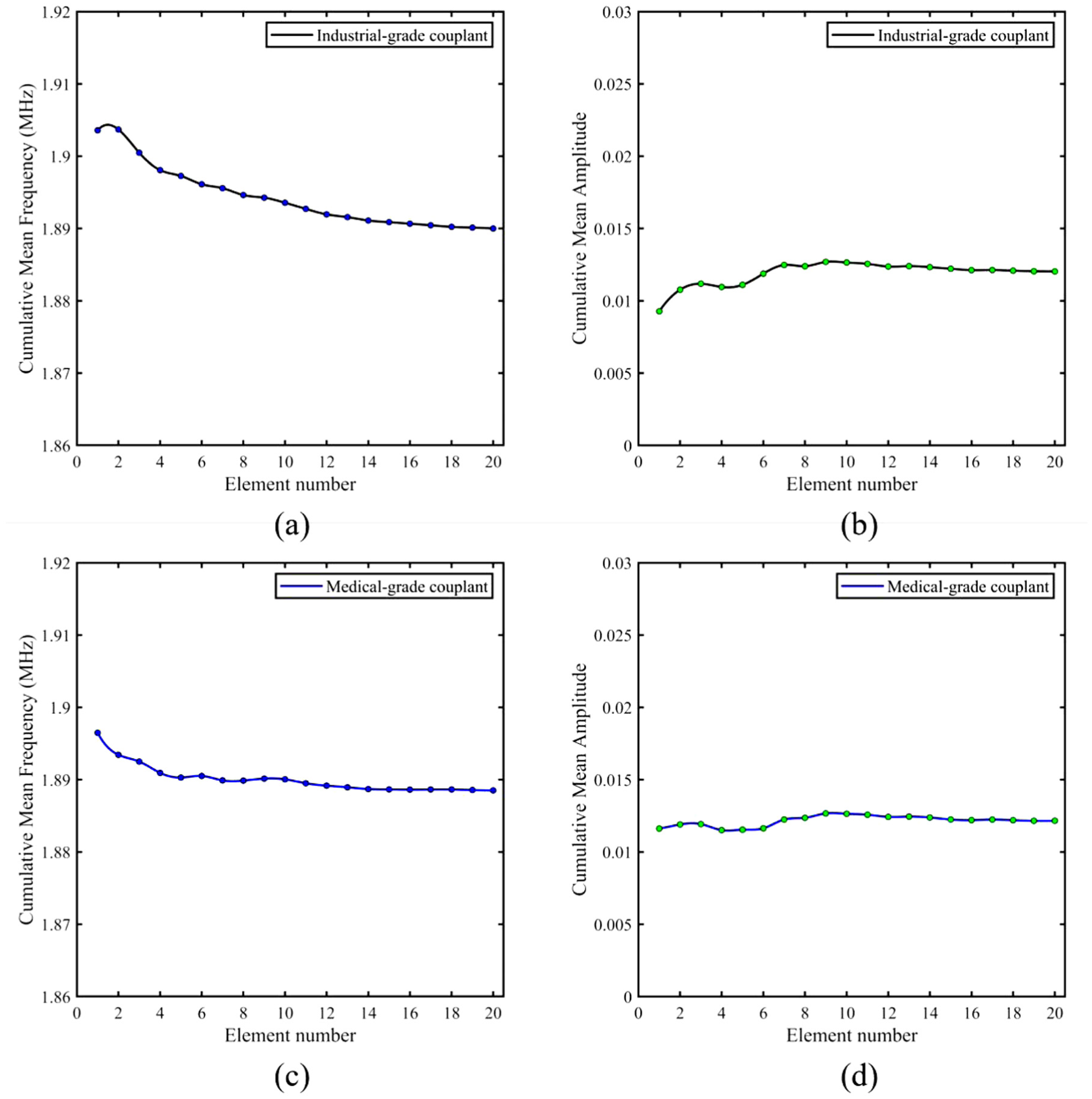
To further identify the excited Lamb modes, signals from the 1st to the 64th elements were subjected to wavenumber-frequency analysis. The results were compared with the theoretical wavenumber-frequency dispersion curves, as shown in Figure 12(c). To mitigate the interference of the initial pulse wave, the analysis was performed over a 3–40 $μ s$ time window. Multiple modes were observed, including A0, S0, A1, S1-ZGV, and S2, with S1-ZGV mode exhibiting the highest amplitude. Figure 12(d) present the wavenumber-frequency analysis conducted within the time range of 22–40 $μ s$ to exclude interference from other Lamb wave modes. The analysis confirms the exclusive presence of S1-ZGV and thickness resonance modes, with the S1-ZGV mode showing better energy concentration. Although these results validate single-element excitation of the S1-ZGV mode, two key limitations remain: interelement inconsistency and short resonance duration. These challenges will be addressed by the proposed TDS and PA excitation techniques.

Prior to investigating the TDS method and PA technique, it is essential to examine how the variation patterns of ZGV modes and differences in coupling characteristics affect the ZGV response. A linear transducer with 128 elements was placed on an intact thin plate, with all elements separately exciting and receiving signals. To further study the influence of acoustic coupling, two types of ultrasonic couplants were applied: a medical-grade couplant and an industrial-grade couplant. Figure 13 presents the ZGV frequency and amplitude variation curves obtained by performing FFT on the signals from all 128 elements using a time window of 6–40 μs. The black solid line corresponds to the industrial couplant, and the blue solid line represents the medical couplant.

Figure 13.

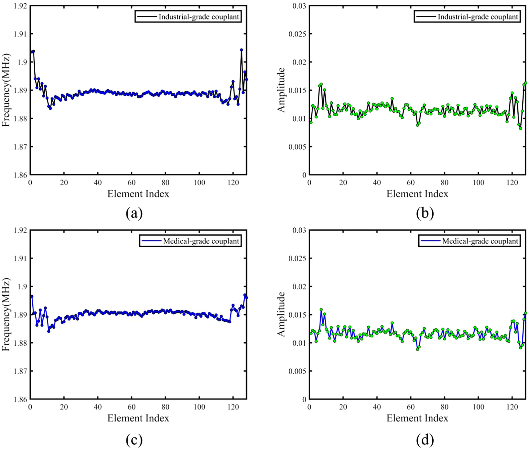
ZGV frequency and amplitude for all elements under separate excitation and reception with two different coupling agents; Industrial couplant: (a) ZGV frequency and (c) ZGV amplitude; Medical couplant: (b) ZGV frequency and (d) ZGV amplitude.

The results indicate that both the ZGV frequency and amplitude follow highly consistent variation trends regardless of the couplant used. In both scenarios, the edge elements of the array exhibit greater fluctuation, whereas the central elements remain relatively stable—a pattern likely attributable to inherent inconsistencies among the transducer elements themselves. Further examination of the ZGV frequency magnitudes shows that, after excluding outliers with significant deviations, nearly all frequencies converge around 1.89 MHz. Similarly, ZGV amplitude variations are minor, with all values lying within the range of 0.005–0.02 MHz. Nevertheless, amplitude is not a primary concern in this study, as it was not employed for actual thickness measurement. In summary, differences in coupling characteristics between the transducer and the plate do not lead to substantial fluctuations in ZGV values; rather, variations appear to arise mainly from inconsistencies in specific transducer components. Building on these findings, the subsequent sections will focus on enhancing and optimizing the ZGV measurement through the application of the TDS method and PA technology.

S1-ZGV frequency extraction by TDS

Acoustic attenuation over propagation distance during experimentation hindered the identification of distinct resonance frequency of S1-ZGV mode,⁴³ accompanied by inconsistencies across individual elements of the linear PA transducer. Moreover, the finite width of transducer elements, unlike idealized point source in simulations, introduces difference in S1-ZGV mode excitation and reception. The TDS method can effectively address these challenges by utilizing signals from multiple receivers to extract resonance frequencies. However, the parameter $n$ (element number) should be optimized prior to TDS implementing.

Signals were acquired sequentially from the 1st to the 64th element with excitation at the 1st element. Spatial Fourier transform analysis, as shown in Figure 14(a), reveals that S1-ZGV Lamb waves exhibit a source-centered energy distribution and periodic with the half-wavelength of the S1-ZGV mode. Consequently, elements within the half-wavelength range were selected for TDS processing. Periodicity analysis incorporating transducer pitch and element width determined four elements as optimal.

Figure 14.

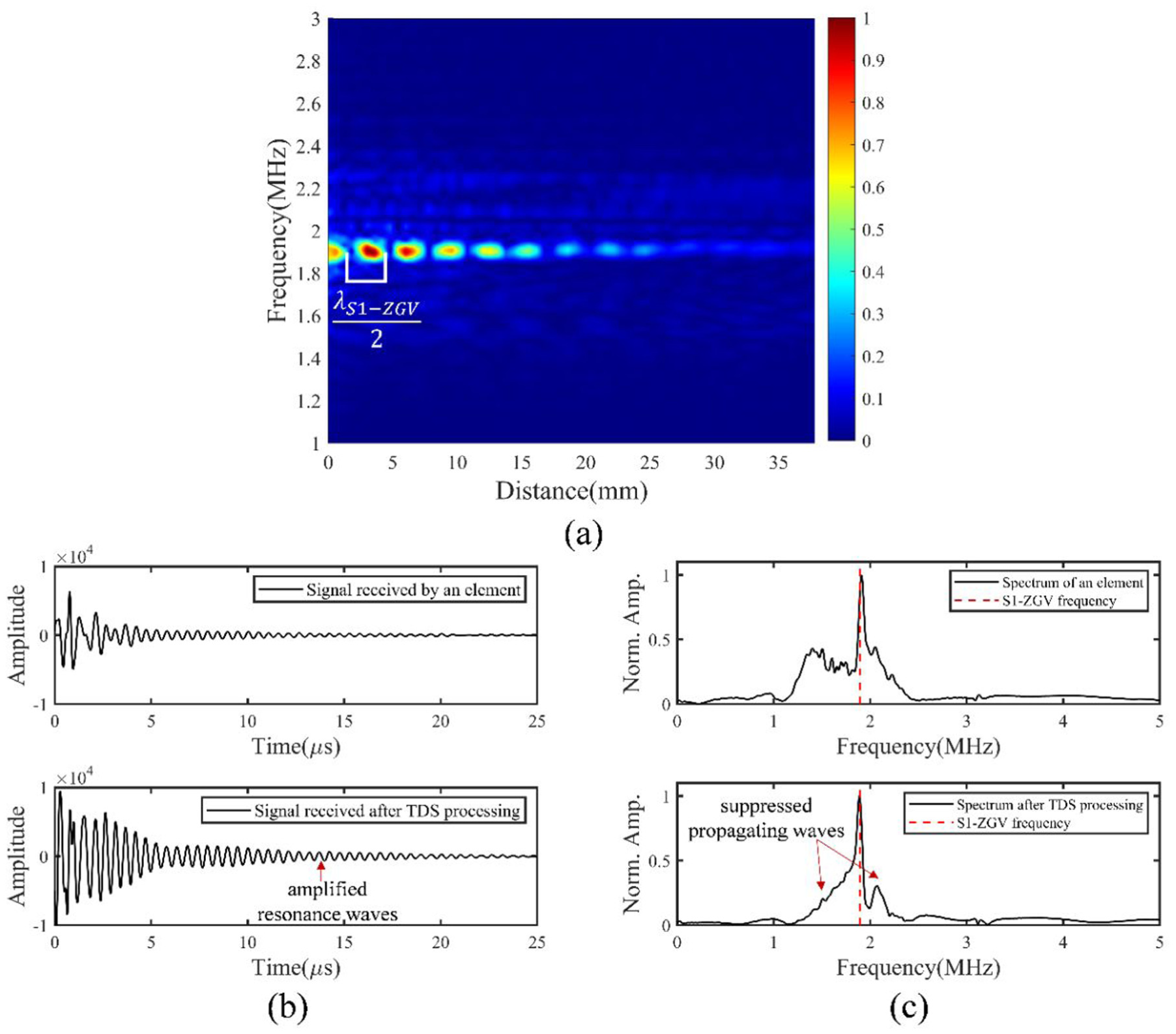
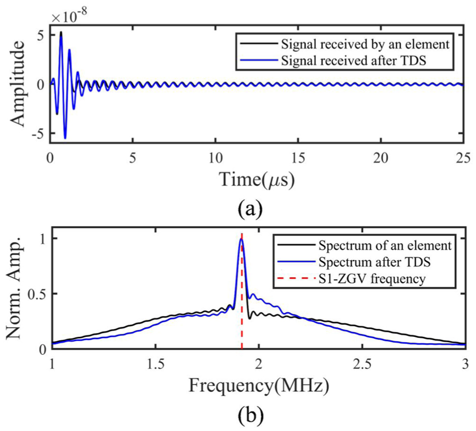
(a) Experimental spatial spectra of S1-ZGV mode and (b) A-scan signal and (c) spectra comparison before and after TDS process.

Figure 14(b) and (c) compares single-element and TDS-processed signals. For the spectral analysis, a time window covering the full duration of the acquired signal (0–25 μs) was applied to the FFT. Time- and frequency-domain results demonstrate that inherent suppression of propagating waves and enhanced alignment of resonance peak with the theoretical S1-ZGV frequency (1.8928 MHz, red dashed line). TDS processing reduced the peak frequency from 1.9097 to 1.8884 MHz, lowering relative error from 0.89% to 0.23%. Thus, TDS can enhance the efficiency of frequency extraction.

PA-ZGV optimization

To enhance the S1-ZGV mode while suppressing other extra Lamb wave modes, a time delay was introduced as defined by Equation (8). The delay gradient $t_{0} = 55.25 ns$ was determined based on the phase velocity $C_{ph, S 1 - ZGV} = 10, 860 m / s$ . Experimentally, a delay of 55 $ns$ was used due to 1 ns resolution limit of PA ultrasound system. The parameters of the linear PA transducer should be optimized accordingly.

The number of excitation elements was investigated by analyzing the resonance frequency and amplitude of the S1-ZGV mode. Excitation was performed with different numbers of elements (ranging from 1 to 20), and signal was received by the adjacent element (e.g., excitation on elements 1–3, reception on element 4). Resonance waveforms were captured, truncated with 6–40 $μ s$ window, and analyzed using FFT. Two couplants were used in this part of the study. Figure 15 presents the resonance frequencies and amplitudes for different excitation element configurations. The black and blue solid lines show the results using the industrial and medical couplants, respectively. The resonance frequency stabilizes progressively as the number of excitation units exceeds ten, fluctuating within ±0.1 % of the theoretical S1-ZGV frequency (marked by the red dashed band). Although a limited number of measured points fall slightly outside this range, their deviation does not significantly affect the subsequent selection of the excitation array size. While the industrial couplant exhibits slightly larger fluctuations than the medical couplant, both follow nearly identical trends in resonance frequency variation. For both couplants, the ZGV peak amplitude is maximized when 12 excitation elements are employed, corresponding to the highest spectral SNR observed. Accordingly, an excitation array size of 12 elements was selected for all subsequent measurements. It is important to note that the selection of excitation elements is material-dependent and should be re-optimized if material or transducer is changed.

Figure 15.

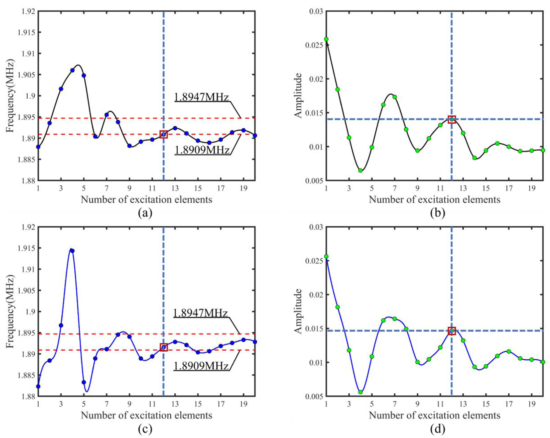
Variation of resonance frequency and amplitude of S1-ZGV mode as a function of the excitation element number; Industrial couplant: (a) frequency and (b) amplitude; Medical couplant: (a) frequency and (b) amplitude.

Further, we examined whether cumulative averaging of ZGV frequency and amplitude across multiple signals could produce comparable frequency characteristics. Each of the first 20 elements was used in turn for excitation and reception, and the corresponding signals within the 6–40 μs time window were processed using the FFT. For the first element, the ZGV frequency and amplitude were taken directly from its own signal. For the second element, the reported values were the average of the first two elements, and so on—thus generating a cumulative moving average over successively included elements. The results in Figure 16 indicate that cumulative averaging promotes rapid convergence of both ZGV frequency and amplitude to stable values. This method, however, remains highly sensitive to inconsistencies across array elements. As shown in Figure 16(a), convergence requires a relatively large number of measurements, primarily because ZGV signals acquired by several of the earlier elements exhibit substantial fluctuations. While the averaging process smooths the resonance frequency and amplitude over multiple measurement positions, it operates differently from the PA approach. The PA technique enhances ZGV mode excitation mainly through controlled time-delay steering of the wavefront, which yields stronger and more stable ZGV signals even in regions with significant reflections or scattering. Consequently, the cumulative averaging method cannot achieve comparable frequency characteristics obtained with the approach proposed in this study.

Figure 16.

S1-ZGV frequency and amplitude cumulative average variation patterns; Industrial couplant: (a) frequency and (b) amplitude; Medical couplant: (a) frequency and (b) amplitude.

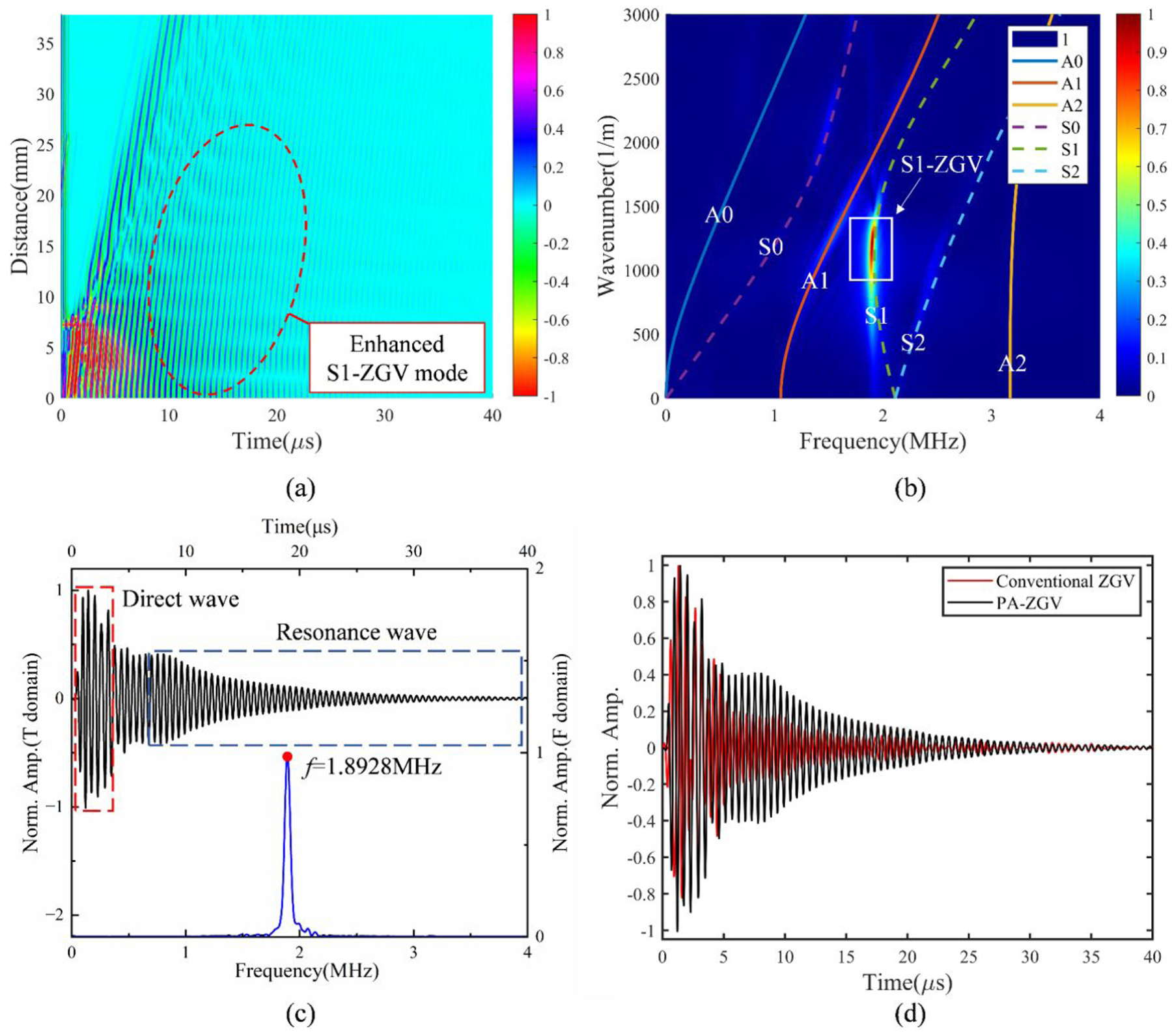
PA excitation with 12 elements significantly enhanced the energy of S1-ZGV mode, as demonstrated in the B-scan shown in Figure 17(a). Clear resonance signals were observed after direct waves, which was also enhanced. Wavenumber-frequency analysis was performed on the received signals within a 3–40 $μ s$ time window (Figure 17(b)), confirming the suppression of A0, S0, and A1 modes with an enhanced S1-ZGV mode, thereby validating the theoretical prediction and the simulations in S1-ZGV mode identification and enhancement. Figure 17(c) shows the signal received by element 13, truncated with 6–40 μs window, and analyzed using FFT, with the corresponding spectrum being nearly free of sidelobes. A comparison of waveforms with the single-element excitation, shown in Figure 17(d), demonstrates an extended resonance duration.

Figure 17.

Results of PA excitation by 12 elements with a delay of 55 ns: (a) B-Scan, (b) wavenumber-frequency analysis, (c) time-domain signal and resonance spectra received by element 13, and (d) resonance waveform comparison with conventional ZGV method.

Optimization of edge signals by TDS and PA

In practical inspection scenarios, transducers are frequently positioned near the edges of test specimens to detect defects. Under such conditions, the extraction of ZGV Lamb waves is significantly complicated by the presence of strong edge-reflected waves. During spectral analysis via the FFT, these boundary-induced wave components are also captured and are difficult to isolate or eliminate through conventional time-window sampling. The two strategies proposed in this study—the TDS method and the PA method—effectively mitigate this issue, thereby facilitating the subsequent isolation of ZGV modes in the frequency domain. To validate their efficacy under realistic edge-reflection conditions, experiments were conducted with the transducer located at the specimen edge. Detailed comparative analyses were then performed on the A-scan signals and corresponding frequency spectra obtained from single-element excitation, TDS processing, and PA processing scenarios.

In the experimental setup, the 13th element of the transducer was used for single-element excitation and reception. For the TDS method, the same element served as the exciting element, while signals were received from elements 13 through 16. In the PA configuration, elements 1 to 12 were excited, with element 13 acting as the receiver. All receiving elements were positioned near element 13 to ensure experimental consistency. As shown in Figure 18(a), the A-scan signal from single-element excitation clearly exhibits multiple wave packets arising from edge reflections. For spectral processing, a time window of 6–40 μs was applied in the FFT for both the single-element and PA methods, whereas the TDS method used a window of 0–40 μs. The corresponding spectrum in Figure 18(b) displays several peaks, including two sharp resonance peaks of nearly equal amplitude near the ZGV frequency, which complicates the unambiguous identification of the ZGV mode. In contrast, the A-scan signals for the TDS method (Figure 18(c)) show a clear suppression of boundary-reflected wave packets. The associated spectrum in Figure 18(d) reveals reduced contributions from both propagating and edge-reflection components, leaving only one resonance peak. This enables rapid and accurate identification of the ZGV mode through spectral analysis, representing an improvement over the single-element approach. Figure 18(e) presents the A-scan signal obtained with the PA method, which exhibits a resonant signal with uniform amplitude variation and virtually no edge reflection signal. The optimization is further evident in its spectrum (Figure 18(f)), where only a single sharp resonance peak remains and spectral components near the ZGV frequency are minimal. This result indicates that the signal acquired with PA at the specimen edge is close to that free from boundary interference, demonstrating the most effective optimization among these methods. In summary, both the TDS and PA methods enhance the robustness of ZGV-mode detection in the presence of edge reflections, thereby improving measurement accuracy for thickness-loss assessment in thin plates.

Figure 18.

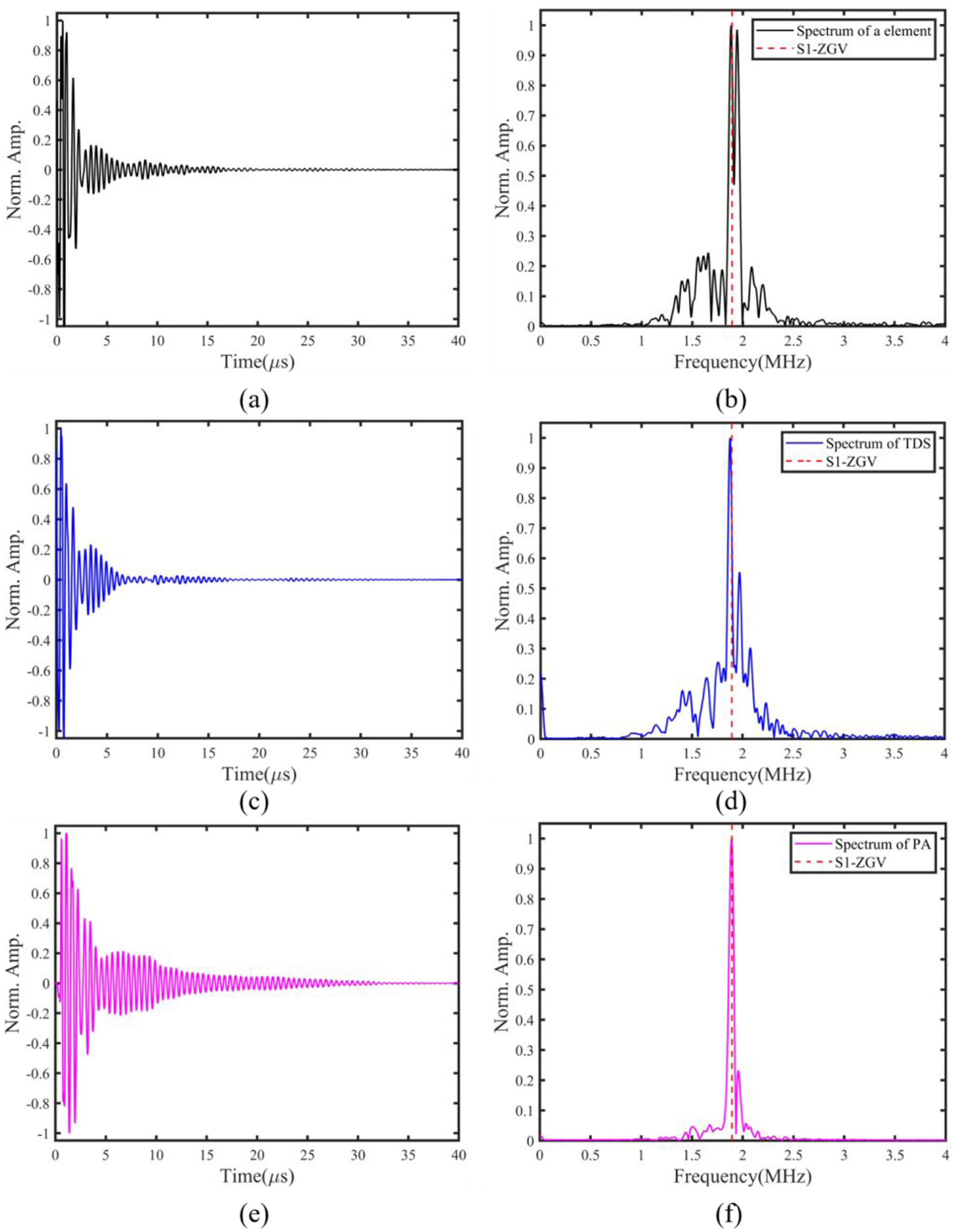
A-scan signals acquired at the specimen edge for (a) single-element ZGV, (c) the ZGV-TDS method, and (e) the PA-ZGV method, with their corresponding spectra shown in (b), (d), and (f), respectively.

Comparative validation experiments

To validate thickness profiles derived from the proposed four ZGV based method, high-frequency PE and line-laser scanning^53,54 were employed as reference methods. These techniques provide high-precision thickness measurement essential for experimental verification. Given machining-induced thickness variations across the workpiece, measurements were taken at five positions (Position 1–5) along the groove.

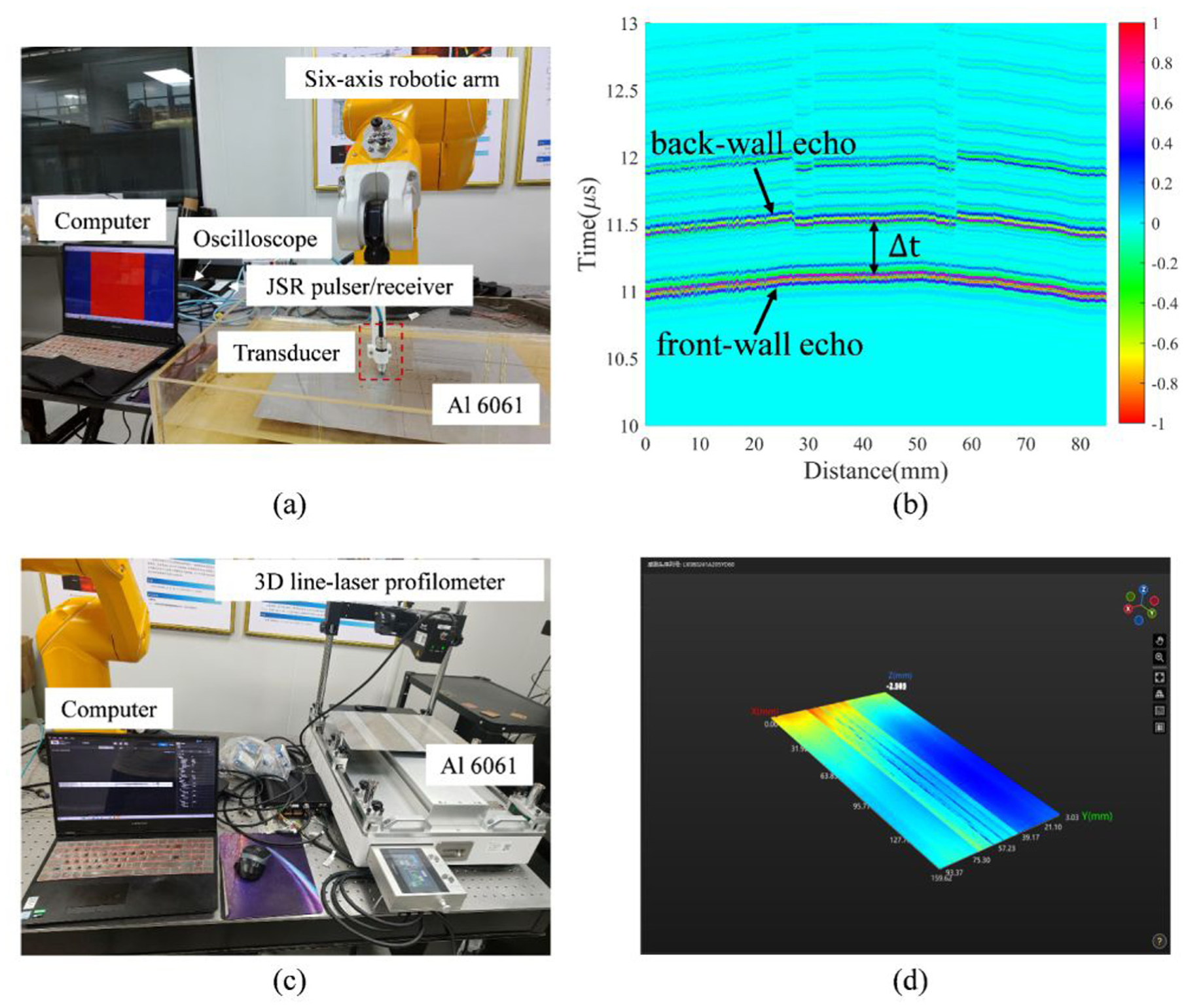
Figure 19(a) shows the PE experimental setup. A 20 MHz immersion transducer was mounted on a Stäubli TX2-60robotic arm transmitted/received signals via a JSR PureView Pulser/Receiver (JPV-PR-USB-Ua1). The corresponding wavelength $λ \approx 0.318 mm$ , is much smaller than the plate thickness, ensuring the pure bulk-wave behavior. The robotic arm scanned linearly over an 84 mm length with a step size of 0.1 mm, while signals were amplified (20 dB) with a sampling rate of 500 MHz. Figure 19(b) shows a representative B-scan, exhibiting distortion from manufacturing-induced flexural deformation of the thin-walled plate. The time difference $Δ t$ of the front-wall and back-wall echoes was calculated to determine the thickness.

Figure 19.

Setup for validation experiments: (a) high-frequency ultrasonic PE method and (b) its typical B-scan signal, (c) line-laser scanning method, and (d) the scanned result.

Figure 19(c) shows the experimental setup for line-laser scanning with Figure 19(d) illustrating the scanning interface. The 3D line-laser profilometer (MECH MIND, Mech-Eye LNX-8080) achieves resolution of 23.5 $μ m$ (x-axis), 23.5 $μ m$ (y-axis), and 0.5 $μ m$ (z-axis). Surface profiles at five locations were scanned. Point cloud data were exported by software Mech-Eye Viewer, and processed in CloudCompare with pass-through filtering to eliminate background noise and external disturbance. Finally, the filtered data were used to generate the thickness profile.

Four ZGV profiling methods were employed. The conventional ZGV sequentially excited and received at each element in the PA transducer. The ZGV-TDS excited the ith element and received from the ith to (i + 3)th element, followed by TDS. The PA-ZGV excited 12 elements (from i to i + 11) with a delay of 55 ns and received the (i + 12)th element. The PA-ZGV-TDS excited 12 elements (from i to i + 11) with a delay of 55 ns and received from the (i + 12)th to (i + 15)th elements, followed by TDS. All the four ZGV methods preform electronic scanning across the whole PA transducer to reconstruct thickness profiles. At each position, thickness was calculated using the ZGV frequency-thickness product relation.

Results and discussion

Figure 20 compares measured thickness profiles at third groove position obtained via the four ZGV methods, PE, and line-laser scanning. The results indicate that the groove defects were accurately reconstructed by all four ZGV methods. However, relatively larger deviations occur near the groove edges due to tip scattering. In addition, the inaccuracies in these localized thickness transition measurements do not affect the overall reconstruction of the groove.

Figure 20.

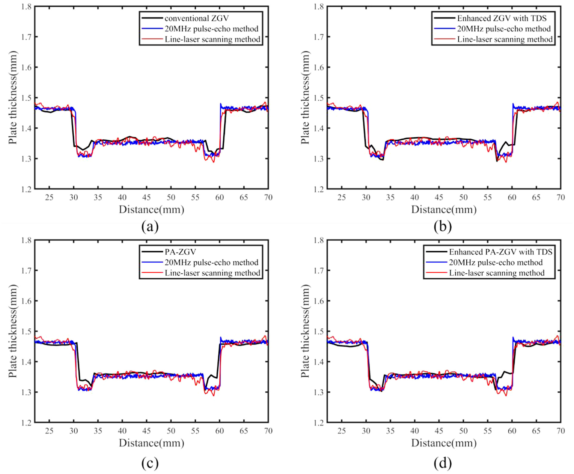
Results comparison between four ZGV Lamb waves methods with high-frequency PE and line-laser methods: (a) conventional ZGV, (b) ZGV-TDS, (c) PA-ZGV, and (d) PA-ZGV-TDS.

Building on the findings from Optimization of edge signals by TDS and PA, which demonstrated that the TDS method and PA technique facilitate the identification and extraction of ZGV modes in strong reflection zones, the transducer was placed 1 cm from the upper edge of the test block to reconstruct a groove profile. This setup allows a further evaluation of the advantages and limitations of the four ZGV methods under such challenging conditions. Figure 21 displays the groove-reconstruction curves obtained at the edge position using the four ZGV methods, the PE method, and the line laser scanning method. For the single-point ZGV method, the reconstructed thickness profile exhibits pronounced oscillations within the groove region, likely due to the adverse influence of boundary reflections on the formation and extraction of the ZGV mode. The ZGV-TDS method, while still showing some fluctuations at specific points, demonstrates clear improvement over the single-point approach. In contrast, the PA-ZGV and PA-TDS methods yield reconstructed thickness curves with significantly fewer fluctuations, indicating substantially enhanced robustness in ZGV extraction under strong reflection interference. These observed differences align consistently with the analysis of ZGV signals in edge regions presented in Optimization of edge signals by TDS and PA.

Figure 21.

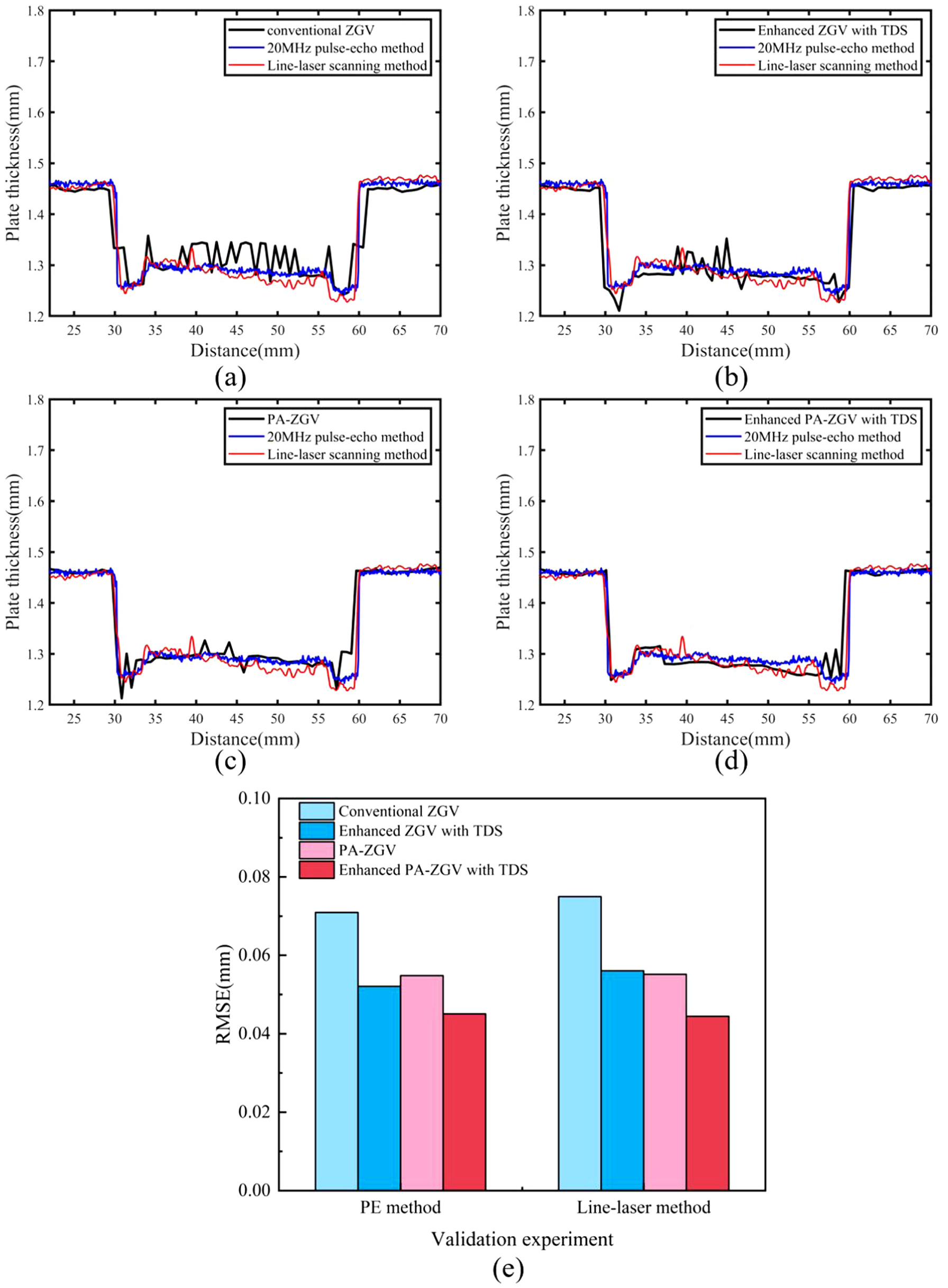
Comparison of four ZGV methods versus high-frequency PE and line-laser techniques at the specimen edge: (a) conventional ZGV, (b) ZGV-TDS, (c) PA-ZGV, (d) PA-ZGV-TDS, along with (e) RMSE analysis.

To further quantify the measurement accuracy, RMSE between these four methods and two reference methods were calculated. As illustrated in Figure 21(e), the RMSE values for groove-profile reconstruction obtained with PA and TDS techniques are consistently lower than those achieved using the single-point ZGV method. Specifically, the single-point ZGV method yields RMSE values exceeding 0.07–0.0709 mm relative to the PE method and 0.0750 mm relative to line-laser scanning. In comparison, both the ZGV-TDS and PA-ZGV methods produce comparable RMSEs, which remain within the range of 0.05–0.06 mm. The PA-ZGV-TDS method further reduces the RMSE below 0.05 mm, with values of 0.0451 and 0.0445 mm against the two reference techniques, respectively. This quantitative RMSE analysis clearly demonstrates that incorporating either PA technology or the TDS method enhances measurement accuracy at specimen edges. Moreover, it confirms that the combined PA-ZGV-TDS approach enables high-precision reconstruction of residual-thickness profiles even in regions dominated by strong reflections.

The applicability of the method was further assessed through systematic measurements at five representative locations on the thin plate, followed by a quantitative comparative analysis. Figure 22(a) and (b) shows that RMSE values between each ZGV method and the reference methods across the five positions. Line-laser results represent ground truth, confirming the accuracy of the ZGV methods. All RMSE values remains below 0.035 mm, demonstrating that low-frequency (around 2 MHz) ZGV measurements achieve comparable results with high-frequency (20 MHz) PE method. Figure 22(c) summarizes the mean RMSE for each ZGV method. All means are below 0.03 mm, confirming high accuracy relative to actual residual thickness. Compared to the high-frequency PE method, the mean RMSE values for the four ZGV methods are 0.02556, 0.02649, 0.02475, and 0.02190 mm, respectively. Compared to line-laser scanning, the corresponding values are 0.02880, 0.02796, 0.02170 and 0.02362 mm, respectively.

Figure 22.

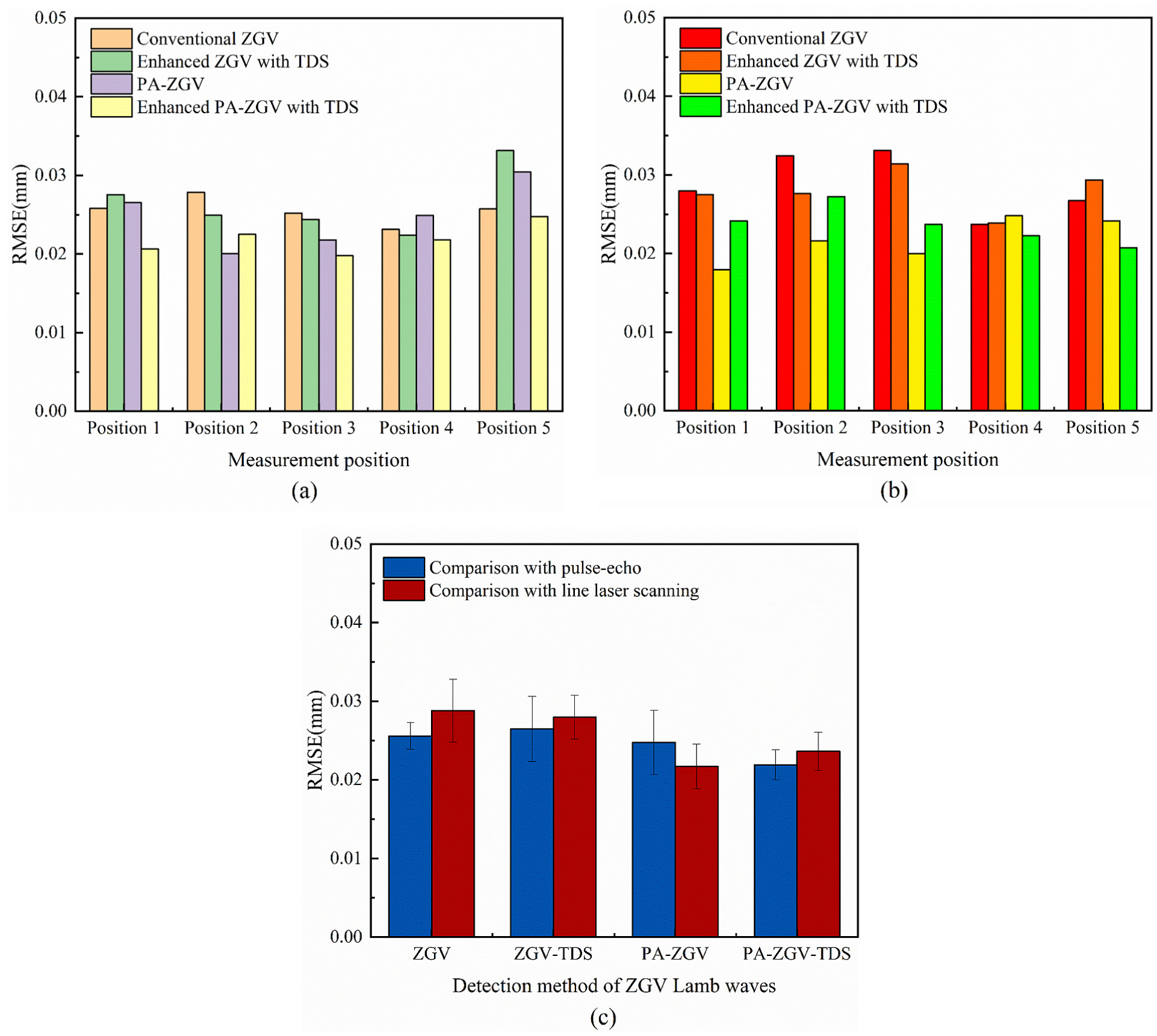
RMSE of ZGV lamb waves methods compared to (a) conventional PE method and (b) line-laser method; along with (c) mean values.

Overall, all four ZGV-based methods achieved reliable reconstruction at the five representative positions, with mean RMSE values below 0.03 mm. Under benign central-region conditions, the differences among the four methods are limited. Nevertheless, the PA- and TDS-enhanced strategies improve measurement robustness under more challenging conditions. Specifically, ZGV-TDS eliminates the need for time-domain truncation of resonance signals and stabilizes frequency extraction through multireceiver summation. PA-ZGV improves spectral purity by selectively enhancing the S1-ZGV mode, while PA-ZGV-TDS combines both advantages, exhibiting the smallest RMSE variation (±0.0024 mm) and improved performance in reflection-prone regions. Consequently, PA-assisted ZGV methods provide accurate and operationally efficient solution for thin-plate thickness mapping.

While the above results demonstrate the effectiveness of the proposed methods under the present experimental conditions, the practical applicability of the approach should also be interpreted within a clearly defined scope. The experimental validation was conducted only on thin isotropic aluminum plates with machined groove defects. Therefore, the current results should be regarded as a proof-of-concept demonstration for robust local residual-thickness profiling in such structures. The proposed thickness reconstruction relies on the S1-ZGV frequency–thickness relationship for a given material system. Consequently, uncertainties in elastic wave velocities or material property may introduce systematic bias in the absolute thickness estimation. Although moderate couplant variations were shown to have only a weak influence on the extracted ZGV frequency in the present configuration, more severe coupling variations, nonideal surface conditions (e.g., roughness or oxidation), and degraded local contact conditions may still reduce spectral SNR and affect the robustness of frequency peak extraction. Furthermore, more complex scenarios, including curved geometries, multilayer plates, and anisotropic materials, may alter the local dispersion characteristics and mode-conversion behavior. In such cases, the frequency–thickness mapping must be recalibrated, and the phased-array excitation as well as TDS parameters may require case-dependent re-optimization.

Conclusion

This study introduces a method for quantifying thickness loss in thin plates using ZGV Lamb waves generated by PA technology. The principles of thickness measurement were established based on the sensitivity of the S1-ZGV mode to variations in wall thickness, as evidenced by shifts in resonance frequencies. A mathematical derivation of the PA excitation technique showed that optimized time-delay laws significantly enhance the intensity of the S1-ZGV mode. Additionally, a TDS method was proposed to eliminate the need for time-domain truncation, thereby improving data processing efficiency. Four ZGV-based methods for thickness profile reconstruction were developed and validated through simulations. Experimental investigations using a linear PA transducer confirmed effective excitation of the S1-ZGV mode. PA excitation with 12 elements and a delay of 55 ns prolonged resonance durations, resulting in enhanced excitation of the S1-ZGV mode. Validation against high-frequency pulse-echo (PE) and line-laser scanning methods demonstrated an average RMSE of less than 0.03 mm. The PA-ZGV-TDS method demonstrates the most stable performance under reflection-prone conditions, while differences among the four ZGV-based methods remain relatively small in benign central-region measurements. Moreover, they achieved accuracy comparable to traditional 20 MHz high-frequency PE technology, despite operating at a much lower frequency of 2 MHz. Thus, the proposed method provides a sensitive and efficient solution for assessing structural thickness loss. Future work will focus on adaptive element selection strategies, robust performance in reflection-prone regions (e.g., specimen edges), and extending the methodology beyond thin isotropic plates to more complex and practically relevant scenarios, including multilayer and anisotropic materials, variable surface and coupling conditions, and complex geometries.

Footnotes

ORCID iD

Maodan Yuan

Funding

The authors disclosed receipt of the following financial support for the research, authorship, and/or publication of this article: This work was supported by Guangdong Basic and Applied Basic Research Foundation [No. 2026A1515011691, 2022A1515240040, 2024A1515030112]; Guangzhou Basic and Applied Basic Research [No. 2024A04J4295]; National Science Foundation of China [No. 52405583], and the China Postdoctoral Science Foundation [No. 2023M740755].

Declaration of conflicting interests

The authors declared no potential conflicts of interest with respect to the research, authorship, and/or publication of this article.

References

Willberg

Koch

Mook

, et al. Continuous mode conversion of lamb waves in CFRP plates. Smart Mater Struct 2012; 21: 9.

Huang

Zeng

Zhang

, et al. Hidden corrosion monitoring via phase shift evaluation of lamb wave modes. Smart Mater Struct 2024; 33: 085022.

Zhang

Huang

Palek

, et al. Glass fiber–reinforced polymer–packaged fiber Bragg grating sensors for ultra-thin unbonded concrete overlay monitoring. Struct Health Monit 2015; 14: 110–123.

Jeong

Kim

Park

, et al. Long-term monitoring method for tunnel structure transformation using a 3d light detection and ranging equipped in a mobile robot. Struct Health Monit 2023; 22: 3742–3760.

Xia

Huang

, et al. Thickness and permeability estimation of metallic plates by triple-frequency eddy-current testing with probe lift-off. IEEE Trans Instrum Meas 2024; 73: 1–8.

Sodano

. Development of an automated eddy current structural health monitoring technique with an extended sensing region for corrosion detection. Struct Health Monit 2007; 6: 111–119.

Linh

NTT

Khang

NHD

Trang

Le Thi Ngoc

, et al. Determining the thickness of a thin aluminum sheet using the transmission measurement of X-rays with varying energies: a comparative analysis between calibration curve fitting and artificial neural network approaches. Nucl Instrum Methods Phys Res A 2024; 1068: 169740.

Mengue

Hage-Ali

Zhgoon

, et al. Direct integration of SAW resonators on industrial metal for structural health monitoring applications. Smart Mater Struct 2021; 30: 125009.

Ahmed

Lee

. Development of autonomous target recognition and scanning technology for pulse-echo ultrasonic propagation imager. Struct Health Monit 2020; 19: 1064–1074.

10.

Lee

Park

. Damage visualization of pipeline structures using laser-induced ultrasonic waves. Struct Health Monit 2015; 14: 475–488.

11.

Livadiotis

Ebrahimkhanlou

Salamone

. Monitoring internal corrosion in steel pipelines: a two-step helical guided wave approach for localization and quantification. Struct Health Monit 2021; 20: 2694–2707.

12.

Maev

Shao

Maeva

. Thickness measurement of a curved multilayered polymer system by using an ultrasonic pulse-echo method. Mater Charact 1998; 41: 97–105.

13.

Kruger

Lord

Monchalin

. Laser ultrasonic thickness measurements of very thick walls at high temperatures. In Thompson

Donald O.

Chimenti

Dale E.

,(Eds.), Review of progress in quantitative nondestructive evaluation. American Institute of Physics, Vols 25a and 25b, 2006, Vol. 820, pp. 240–247.

14.

Zhang

Cegla

. Co-located dual-wave ultrasonics for component thickness and temperature distribution monitoring. Struct Health Monit 2023; 22: 1090–1104.

15.

Wang

Lai

, et al. High-frequency ultrasound-based thickness measurement of highly attenuating materials. Meas Sci Technol 2023; 34: 035004.

16.

Dixon

Lanyon

Rowlands

. Coating thickness and elastic modulus measurement using ultrasonic bulk wave resonance. Appl Phys Lett 2006; 88: 141907.

17.

Zhang

Wang

Zhang

, et al. Nondestructive evaluation of thickness variations for elastic plates by high-overtone bulk acoustic resonance. IEEE Trans Ultrason Ferroelectr Freq Control 2012; 59: 2709–2715.

18.

Lee

Kim

. Elastic metamaterials for guided waves: from fundamentals to applications. Smart Mater Struct 2023; 32: 123001.

19.

Chai

Wang

Liu

, et al. Structural health dynamic monitoring for gear transmission based on guided waves. Smart Mater Struct 2023; 32: 035025.

20.

Satyarnarayan

Chandrasekaran

Maxfield

, et al. Circumferential higher order guided wave modes for the detection and sizing of cracks and pinholes in pipe support regions. NDT E Int 2008; 41: 32–43.

21.

Tzaferis

Tabatabaeipour

Mcmillan

, et al. A shear horizontal phased array steering excitation technique for remnant wall thickness quantification. Ultrasonics 2024; 136: 107142.

22.

Suresh

Balasubramaniam

. Remnant thickness quantification in small thickness structures utilising the cut-off property of a1 lamb wave mode employing linear array elements. J Appl Phys 2022; 131: 174502.

23.

Heinlein

Mariani

Milewczyk

, et al. Improved thickness measurement on rough surfaces by using guided wave cut-off frequency. NDT E Int 2022; 132: 102713.

24.

Tolstoy

Usdin

. Wave propagation in elastic plates–low and high mode dispersion. J Acoust Soc Am 1956; 28: 794–795.

25.

Prada

Balogun

Murray

. Laser-based ultrasonic generation and detection of zero-group velocity lamb waves in thin plates. Appl Phys Lett 2005; 87: 194109.

26.

Prada

Clorennec

Royer

. Local vibration of an elastic plate and zero-group velocity lamb modes. J Acoust Soc Am 2008; 124: 203–212.

27.

Gruensteidl

Berer

Hettich

, et al. Determination of thickness and bulk sound velocities of isotropic plates using zero-group-velocity lamb waves. Appl Phys Lett 2019: 251905.

28.

Sun

. Measurement on a thin plate of stepped thickness using zero-group velocity effect of an s1 mode lamb wave induced by a moving laser source. Appl Opt 2023; 62: 7571–7576.

29.

Ren

Meng

Deng

. Evaluating impact damage on carbon fiber-reinforced polymer plates utilizing zero-group-velocity lamb waves. Smart Mater Struct 2024; 33: 95013.

30.

Liu

Guan

, et al. Advancing measurement of zero-group-velocity lamb waves using PVDF-TrFE transducers: first data and application to in situ health monitoring of multilayer bonded structures. Struct Health Monit 2023; 22: 2641–2650.

31.

Cho

Hara

Matsuo

. Evaluation of the thickness and bond quality of three-layered media using zero-group-velocity lamb waves. J Phys Conf Ser 2014; 520: 012023.

32.

Pan

Shen

Kan

, et al. Determination of each layer thickness of thin bilayer using laser-based multiple zero-group velocity lamb waves. Opt Laser Technol 2023; 165: 109580.

33.

Zhang

Deng

. Modeling and simulation of zero-group velocity combined harmonic generated by guided waves mixing. Ultrasonics 2023; 132: 106996.

34.

Yuan

Liu

Sha

, et al. Zero group velocity feature in CFRP-nomex honeycomb structure and its use for debonding detection. Mech Syst Signal Process 2024; 216: 111479.

35.

Guo

Yin

Deng

. Evaluation of surface corrosion damage in thin plates by zero-group velocity lamb waves based on PVDF comb transducers. Thin-Walled Struct 2024: 112345: 204: 112345.

36.

Meng

Deng

. Experimental validation of zero-group-velocity feature guided waves in a welded joint utilizing the pitch-catch measurement technique with air-coupled ultrasonic transducers. Ultrasonics 2024: 142: 107362.

37.

Yuan

Chen

, et al. Excitation of s1-ZGV lamb wave with a compact wedged transducer and its application in local stress measurement. NDT E Int 2023; 139: 102944.

38.

Luo

Wang

Zhang

, et al. A phased array ultrasonic-based enhanced strategy of critically refracted longitudinal (LCR) wave technique. NDT E Int 2022; 133: 102765.

39.

Xuan

Yuan

, et al. Local stress measurement in thin aluminum plates based on zero-group-velocity lamb mode. Chin J Mech Eng 2023; 36: 31.

40.

Guo

, et al. Simultaneous measurement of thickness and bulk wave velocities of thin plates using laser-excited local ultrasonic resonances. Mech Syst Signal Process 2025; 228: 20.

41.

Xie

Mezil

Otsuka

, et al. Imaging gigahertz zero-group-velocity lamb waves. Nat Commun 2019; 10: 2228.

42.

Sun

. Measurement on a thin plate of stepped thickness using zero-group velocity effect of an s1 mode lamb wave induced by a moving laser source. Appl Opt 2023; 62: 7571–7576.

43.

Ryden

. Enhanced impact echo frequency peak by time domain summation of signals with different source receiver spacing. Smart Struct Syst 2016; 17: 59–72.

44.

Balogun

Murray

Prada

. Simulation and measurement of the optical excitation of the s 1 zero group velocity lamb wave resonance in plates. J Appl Phys 2007; 102: 064914.

45.

Veit

Belanger

. An ultrasonic guided wave excitation method at constant phase velocity using ultrasonic phased array probes. Ultrasonics 2019; 102: 106039.

46.

Verma

Belanger

. Surface breaking crack sizing method using pulse-echo Rayleigh waves. Ultrasonics 2023; 138: 107232.

47.

Verma

Belanger

. An alternative Rayleigh wave excitation method using an ultrasonic phased array. Ultrasonics 2023; 135: 107121.

48.

Cès

Clorennec

Royer

, et al. Thin layer thickness measurements by zero group velocity lamb mode resonances. Rev Sci Instrum 2011; 82: 114902.

49.

De Chimenti Rokhlin

. Relationship between leaky lamb modes and reflection coefficient zeroes for a fluid-coupled elastic layer. J Acoust Soc Am 1990; 88: 1603–1611.

50.

Huang

Zhou

Tian

, et al. Linear thermal-acoustic responses of a composite panel in progressive wave tube based on wavenumber-frequency analysis. J Sound Vib 2018; 443: 1–24.

51.

Ren

Cho

Lissenden

. A guided wave sensor enabling simultaneous wavenumber-frequency analysis for both lamb and shear-horizontal waves. Sensors (Basel) 2017; 17: 488.

52.

Prada

Clorennec

Royer

. Local vibration of an elastic plate and zero-group velocity lamb modes. J Acoust Soc Am 2008; 124: 203–212.

53.

Perez

Matuda

Buiochi

, et al. Self-compensation methodology for ultrasonic thickness gauges. Ultrasonics 2023; 135: 107105.

54.

Hwang

Kim

Lim

, et al. Automated visualization of steel structure coating thickness using line laser scanning thermography. Autom Constr 2022; 139: 104267.