
Abstract
In recent decades, various techniques have been developed to support structural health monitoring (SHM). These approaches have benefited significantly from advances in artificial intelligence and big data, which have enabled the detection of structural damage with increasing accuracy. Although such methods allow for automated and real-time assessment of structural integrity, their deployment is often constrained by hardware requirements because of the high computational demands of machine learning (ML) models. These limitations may hinder the practical implementation of automated SHM systems in real-world scenarios. Although pruning techniques aimed at reducing model size by removing specific components of the neural network have been proposed to address this issue, they often suffer from limitations that may be mitigated through alternative approaches, which remain underexplored. In this study, we propose a novel pruning method that integrates metaheuristic optimization techniques to identify the optimal set of neurons to prune. The proposed approach is evaluated using a real-world case study in which the size of an ML model trained to detect structural damage is reduced. The results show that the proposed technique can reduce the model size by 45%, with only a 0.16 and 0.43% decrease in damage detection performance, measured in terms of F1 score and Area Under Curve (AUC) score, respectively.
Keywords
Introduction
Bridge structural health monitoring (SHM) is a critical activity to ensure public safety, optimize maintenance strategies, and extend the service life of these vital infrastructures. Bridges are subjected to dynamic loads, adverse weather conditions, continuous vibrations, and natural degradation processes over time, all of which can compromise their structural integrity. Early damage detection—even of defects imperceptible to the naked eye—allows informed decision-making regarding preventive or corrective interventions, thereby significantly reducing the costs associated with major repairs or catastrophic failures that could lead to serious human and economic consequences. Furthermore, an efficient monitoring system supports a more sustainable and cost-effective asset management of infrastructure by prioritizing interventions based on the structures’ actual condition.
The ability to obtain automated, real-time information on a bridge’s structural health would not be possible without the advanced instrumentation systems that have been developed over the years. These systems collect as much information as possible from the bridge to feed the algorithms tasked with detecting structural damage signs. Among the collected data are, for example, the dynamic response of the bridge, which is used to assess its behavior under different loading conditions 1 ; environmental variables, such as temperature, humidity, and atmospheric pressure 2 ; and traffic-related information, including vehicle counts and vehicle characteristics. 3 All of these data are measured by the instruments’ sensors and must be transmitted to a server for subsequent processing.
Notably, given the immense amount of data generated when instrumenting a bridge with sensors installed directly on the structure, transmitting this large volume of data can be both challenging and costly. Therefore, in some cases, the instrumentation system may consist of processing nodes rather than simple sensors, where each node includes one or more sensors connected to a processing unit. For example, in the study by Alamdari et al., 4 800 jack arches are equipped with three acceleration sensors and a processing node. This setup allows the direct execution of data analysis algorithms directly at the node, thus facilitating data transmission. However, a key limitation of this approach is that the processing nodes generally have limited hardware capabilities, which can restrict the applicability of certain machine learning (ML) algorithms due to their high computational demands. Consequently, there is a pressing need to reduce these hardware requirements to make ML models lighter and faster.
Although techniques focused on reducing the components of ML models, commonly known as pruning techniques, have been developed to lower hardware requirements, classical pruning methods present several limitations. First, they often rely on fixed heuristics based on pre-established thresholds or local metrics (such as weight magnitude) to determine which neurons or connections to remove. These criteria evaluate the importance of individual components in isolation, without considering how their removal affects the network’s overall behavior across subsequent layers. Furthermore, intensive retraining processes are typically required to recover the precision lost after pruning. 5 In addition, they may struggle with generalization, meaning that a technique effective for a particular architecture or domain may not easily transfer to others.
Despite these well-known limitations, the application of alternative pruning strategies to SHM models remains largely unexplored. As noted in the study by Santos-Vila et al., 6 the scientific community has primarily concentrated on core challenges such as damage detection, modal feature identification, and anomalous data detection—problems that must be solved first to build an effective monitoring system. More recent challenges, including model compression and the deployment of ML algorithms on edge devices with significant hardware constraints, have only recently gained attention as sensor network architectures have evolved toward distributed processing nodes. Consequently, the intersection of metaheuristic optimization and neural network pruning (particularly for autoencoder (AE) architectures commonly used in SHM) remains an open and underexplored research direction.
Considering these limitations, this study proposes a novel pruning technique based on the application of metaheuristic optimization methods, which specialize in solving combinatorial problems while optimizing a given objective function. 7 The objective of employing metaheuristic techniques is to identify the optimal set of neurons to deactivate to minimize precision loss. This new approach seeks to provide an alternative to current pruning methods while establishing a foundation for future research in this field.
The proposed method is compared with classical pruning techniques and evaluated using a real-world case study based on a widely recognized benchmark dataset that is frequently used by the scientific community due to its high-quality vibration data and the diverse range of damage types it includes. 8 Using this dataset, different neural network topologies and various pruning ratios were tested, allowing the ML model to reduce in size while maintaining a high level of structural damage detection performance.
The size of the model was reduced by 45% while preserving the structural damage detection performance, with a precision loss of less than 1%. These results demonstrate that the proposed technique can compete with classical pruning methods and achieve comparable results. Depending on the proportion of pruned neurons, the new technique may not require a subsequent fine-tuning process, which is an almost mandatory step for contemporary pruning methods. This suggests that the proposed method can find a better neuron deactivation configuration than other approaches under certain test conditions.
Contributions of the article
Implementation of a pruning technique using optimization methods: This study proposes a novel pruning technique that uses metaheuristic optimization algorithms and a hybrid approach when using ML models.
A solid empirical analysis using a real-world case study: The proposed technique is validated using data collected from a real-world case study, highlighting the method’s applicability and lending credibility to the research.
A comparative analysis of current techniques: A comparative analysis is conducted, emphasizing the differences between the proposed method and the state-of-the-art pruning techniques and quantitatively evaluating the performance of the proposed method and conventional pruning approaches.
Formulation of the pruning problem as an explicit combinatorial optimization task: The pruning problem is formulated as a combinatorial optimization problem, allowing the application of various methods to search for solutions that satisfy a set of constraints while optimizing an objective function.
Potential for future applications and associated research directions: By identifying different research avenues stemming from the problem addressed and the proposed solution, this work establishes a foundation for further investigations.
The remainder of this paper is organized as follows: the section “Related work” presents and discusses previous works that have explored the application of metaheuristic techniques to prune artificial neural networks (ANNs), highlighting the specific particularities of this study compared to existing approaches. The section “Background” provides a general overview of the techniques used in this study, including AE-type neural networks, a classical pruning method, and the metaheuristic optimization technique. The section “Methodology” offers a detailed description of the proposed pruning technique and explains how it integrates with the experimental baseline damage detection model. The section “Experiments” presents and discusses various quantitative experiments aimed at demonstrating the pruning capabilities of the proposed method. Finally, the section “Conclusion” outlines potential future research directions, highlights the article’s contributions, and summarizes the key conclusions.
Related work
This section provides a detailed analysis of related works, highlighting the strengths and weaknesses of each and highlighting the specific features of the present study compared to previously proposed techniques. This section contextualizes the various contributions of this research and underscores its novelty.
ML models have been well established and constitute a cornerstone of many recent technological advancements. These algorithms have enabled significant progress across a wide range of domains, such as computer vision through convolutional neural networks (CNNs), anomaly detection (through AE architectures), and natural language processing (using transformer-based models). However, the application of such techniques often involves extensive configuration processes that require domain experts to select the best combination of parameters from a large set of possibilities. These processes may include tuning hyperparameters to maximize model performance, selecting filters to remove in a convolutional network to improve classification and generalization capabilities, or determining which weights to prune in a neural network to reduce memory usage. Although such decisions could, in theory, be made through exhaustive trial and error, the time required for such an approach can become prohibitive. Here, metaheuristic optimization techniques come into play. These methods efficiently explore large and complex search spaces to find near-optimal solutions (though not necessarily the global optimum) within a bounded time frame. Metaheuristics operate by intelligently navigating the search space to optimize an objective function, depending on the problem at hand, whether the goal is to maximize performance or minimize resource consumption.
Beyond pruning, metaheuristic techniques have been applied to other aspects of ML pipelines. A prominent example is feature selection, where optimization algorithms are used to identify minimal subsets of features that preserve classification accuracy. Several metaheuristics have been explored for this purpose, including Harris Hawk Optimization, 9 the Grasshopper Optimization Algorithm, 10 and the Whale Optimization Algorithm, 11 with a broader review available in the study by Agrawal et al. 12 Similarly, hyperparameter optimization has benefited from metaheuristic approaches, with studies applying algorithms such as Gray Wolf Optimization, Whale Optimization, Moth Flame Optimization, and Genetic Algorithms to tune ML models across diverse domains.13–15 It is also worth noting that the term “pruning” appears in the literature in contexts unrelated to neural network compression, such as search space reduction in scheduling problems 16 and rule pruning in classification systems,17,18 which further fragments the body of work directly relevant to this study.
Focusing specifically on works that apply metaheuristics to reduce the size of ML models based on neural networks, most existing research primarily targets CNNs. The study by Liu et al. 19 is one of the pioneering works that addresses this issue using optimization techniques. This study introduces a novel meta-learning approach for automatic channel pruning in deep neural networks, employing an evolutionary algorithm (EA). MetaSelection is proposed by Zhang et al. 20 to automatically select convolutional substructures that should be preserved using an EA. Similarly, Tsai et al. 21 presented a method for selecting both the filters to be removed and the pruning ratio (i.e., the network percentage to be eliminated) employing a search economics metaheuristic. A previous study 22 used an EA to consider the specific hardware target for deploying the pruned CNN. Finally, Palakonda et al. 23 presented a comprehensive comparative study of various metaheuristic algorithms proposed in the scientific literature to prune CNNs. This study highlights the significant body of work dedicated to optimization-based pruning techniques while also pointing out the bias toward CNNs, as all the reviewed methods exclusively focus on this type of neural network.
It is important to highlight that the pruning strategies developed for CNNs do not directly translate to AE architectures, as the two differ in several fundamental aspects. In CNNs, parameters are organized into convolutional filters and feature maps, and pruning typically operates at the level of entire filters or channels. Removing a filter eliminates a complete activation map, which structurally alters the tensor dimensions in subsequent layers and may require significant architectural adjustments. In contrast, feedforward AEs are composed of fully connected layers, where pruning targets individual weights or entire neurons, with a comparatively more localized impact on the network. Furthermore, the objectives being optimized differ substantially: CNN pruning aims to preserve classification or detection accuracy, whereas AE pruning must maintain reconstruction quality, meaning that excessive pruning can directly degrade the learned latent representation. This distinction also affects sensitivity, while CNNs exhibit considerable redundancy across filters, making them generally amenable to structured pruning, AEs are more sensitive to the loss of individual neurons, particularly in the bottleneck layer, where each unit plays a more critical role in encoding the input signal. These architectural and functional differences underscore the need for pruning methods specifically designed for AE, rather than relying on techniques originally conceived for convolutional architectures.
In summary, considering all the works discussed in this section, there is clear evidence of the recent limited research activity related to this study’s specific line of inquiry. Although some studies have applied metaheuristic techniques in hybrid approaches combined with ML algorithms, most of the scientific community has focused on other areas, such as feature selection and hyperparameter optimization. Furthermore, when reviewing the concepts of pruning and metaheuristics, the term “pruning” was found to be shared across different problems (such as search space pruning, rule pruning, and pruning principles), further segmenting the body of related work. Additionally, the use of pruning techniques applied to neural networks has not been generalized across different neural network architectures, as most efforts have focused primarily on CNNs. One of the main contributions of this work is the application of such pruning techniques to feed-forward AE networks. Similarly, the proposed techniques were not validated by a generalized use of real-world cases, which often limits previous studies’ practical relevance. In contrast, the use of a real-world case study involving bridge structures to validate the proposed pruning method adds a serious and realistic dimension to the research, strengthening the practical value of this work’s contribution.
Background
The following subsections provide a general description of the SHM process to establish the context necessary for understanding the study’s use case. In addition, an overview of the techniques used in this study is presented, explaining their operational principles and highlighting their key characteristics.
General overview of SHM
The SHM process involves a system designed to assess the condition of a bridge in real time, aiming to detect and classify different types of structural damage. This system primarily comprises the following components:
Instrumentation system: A set of sensors is installed in the structure to collect real-time data regarding the bridge’s response to various stimuli. This system may include different types of sensors, such as vibration sensors that measure the dynamic response of the bridge and temperature and humidity sensors that monitor the environmental conditions of the bridge.
Data transmission system: This system collects the data measured by the installed sensors and transmits them to a central processing unit (possibly cloud-based), where they are stored for further analysis. Notably, in certain monitoring systems, part of the data transmission load is reduced by implementing local processing units. In such cases, the full volume of raw data is not transmitted; instead, data are processed on site, and only structural health metrics are sent to the central system.
Data analysis system: This may be a subsystem of the data transmission system (when local processing nodes are installed in the structure) or a standalone system hosted on separate servers. This system is tasked with processing structural data and computing indicators that describe the bridge’s structural health using various computational techniques.
Visualization system: This system compiles and presents all metrics and indicators calculated by the implemented algorithms in a human-readable format. Its main goal is to support decision-making processes related to the structure’s maintenance and management.
Machine learning techniques
Advances in ML techniques have significantly enhanced the SHM process of bridges. A wide variety of ML methods have been employed to support the automatic damage detection process; some examples include support vector machines, ensemble algorithms, ANNs, and deep learning techniques. The latter two are particularly notable for their application in unsupervised damage detection tasks.
Autoencoders
An AE is a type of neural network that encodes an input of length


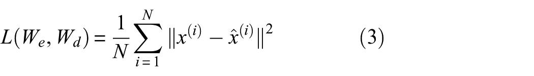
Here,
Topology of an AE. AE: autoencoder.
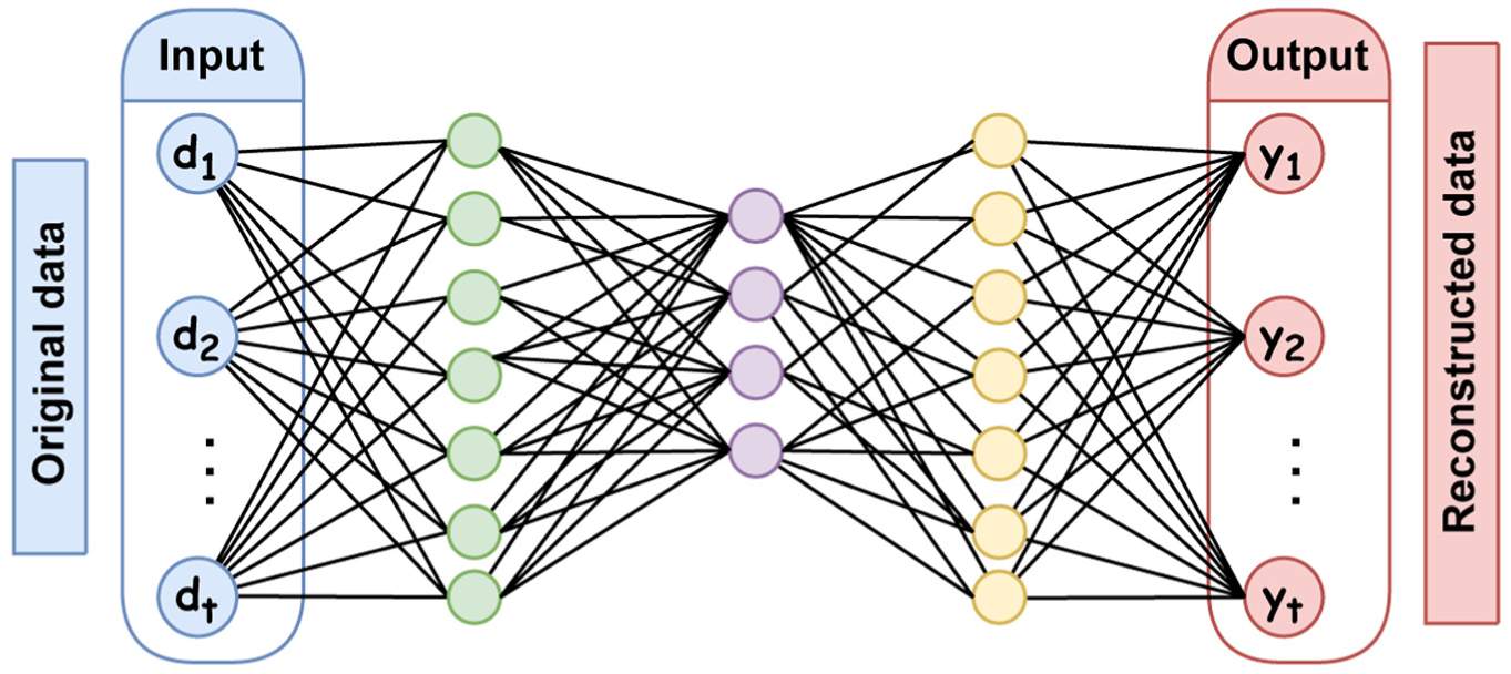
Pruning techniques
Pruning techniques primarily focus on selecting a subset of connections or entire components (e.g., full filters in convolutions, channels, neurons, or even layers). Structured local pruning is a well-known method widely used in the scientific community. 24 This approach reduces model size by eliminating entire structures within the network architecture (Figure 2) rather than removing individual connections, as in unstructured pruning. Unlike other structured approaches that apply pruning decisions at a global level (e.g., evaluating the relative importance of all filters across the entire network and then removing a global percentage), structured local pruning makes local decisions, that is, it evaluates and prunes elements within each layer independently.
Example of pruning a neural network: (a) base model and (b) pruned model.
In this approach, the importance of structured elements (such as filters or channels) within each layer is assessed, and those considered less relevant according to a given metric are removed. The L1 or L2 filter norm, gradient sensitivity, or contribution to the loss function are some common metrics used for this evaluation. The main advantages of this approach are its simplicity and ease of implementation, as it eliminates the need to compute relative importance across the entire network. Furthermore, it produces models that maintain a dense structure, allowing the use of hardware acceleration and optimized libraries for efficient inference. However, making purely local decisions may lead to global suboptimality: that is, it may remove locally insignificant structures that play a critical role in the model’s overall performance along with others.
Combinatorial optimization techniques
Combinatorial optimization is concerned with finding the best solution within a finite but potentially huge set of possible configurations. These problems are often Non-deterministic Polynomial-time hard (NP-hard), meaning that solving them exactly through deterministic algorithms becomes practically infeasible as the problem size grows. Owing to the high computational cost of exactly solving these problems, a set of techniques known as metaheuristics has been developed. Metaheuristics are general-purpose search algorithms (hence the prefix meta) that are designed to efficiently explore the search space and find solutions close to the optimum. Unlike exact methods, metaheuristics do not guarantee the global optimum, but they are particularly useful when the search space is large, nonlinear, discontinuous, or poorly understood, allowing for good solutions to be found within reasonable computational time.
Among the most widely known metaheuristics are:
Genetic algorithms (GA): Simulate the natural evolution process through operators such as selection, crossover, and mutation. 25
Particle swarm optimization (PSO): Inspired by the collective behavior of systems such as bird flocks or fish schools, PSO solutions are dynamically adjusted based on individual and group experiences. 26
Simulated annealing: Mimics the physical annealing process of materials, allowing the search to probabilistically escape local optima.27,28
Ant colony optimization: Based on the behavior of ants searching for optimal paths, it is particularly useful in routing and graph-related problems. 29
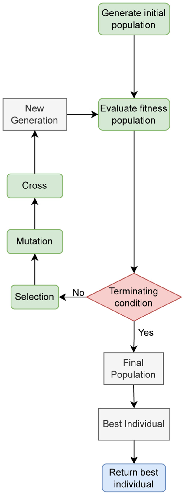
The search process typically comprises two phases: exploration and exploitation. The technique focuses on examining different search space regions in the exploration phase to identify promising areas. During the exploitation phase, promising regions are intensively examined to refine the solutions. Each metaheuristic generates the initial solution, determines stopping criteria, creates new individuals or populations, and balances exploration and exploitation. These characteristics enable the algorithm to adapt its search behavior to the problem landscape.
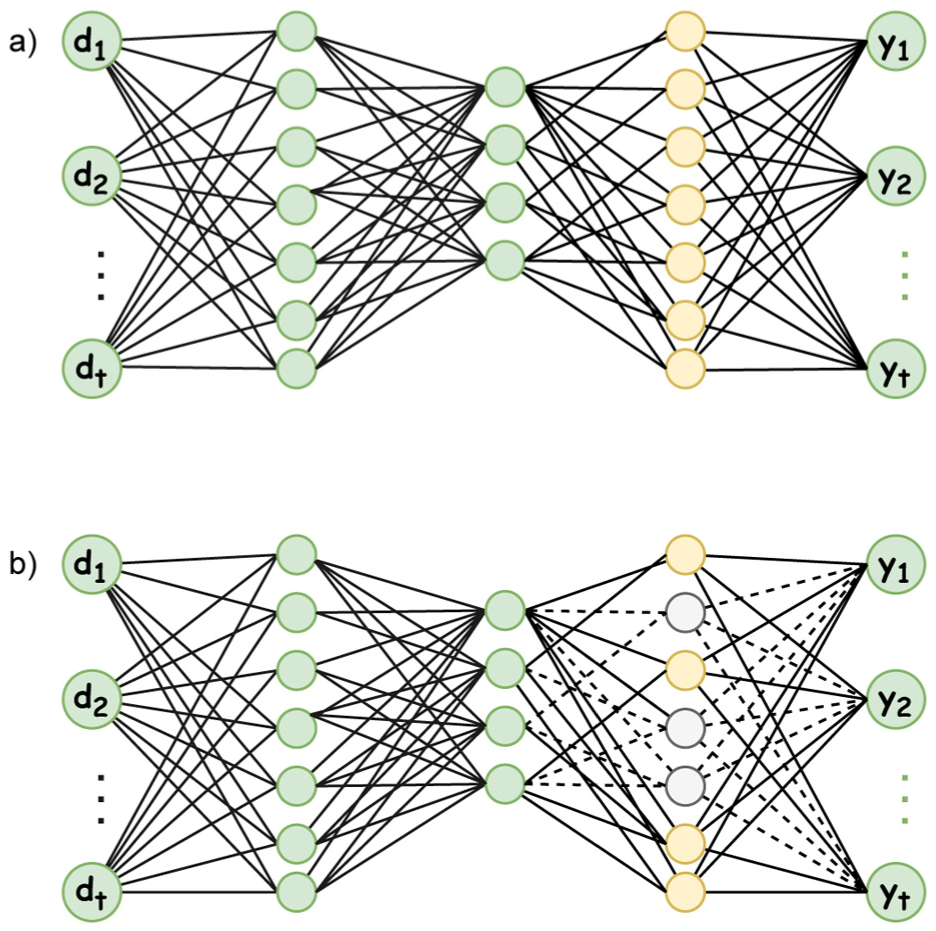
Genetic algorithm
These types of techniques have been successfully applied in a wide range of applications, including circuit design, 30 scheduling, 31 bioinformatics, 14 and, more recently, in ML problems such as feature selection, 32 hyperparameter optimization, 33 and neural network structuring. GA is characterized by its basis in the natural selection process, mimicking biological evolution to find optimal solutions within the search space. Figure 3 presents a schematic explaining the general process followed by the metaheuristic to select the best configuration. Some notable features of this metaheuristic include the following:
It belongs to a class of metaheuristics known as population-based algorithms, meaning that each iteration maintains a set of solutions (referred to as the population) that evolves throughout the search process.
It iteratively improves the solutions (referred to as individuals within the GA context), generating successive generations of increasing quality.
It comprises three fundamental operations: selection, crossover, and mutation.
Selection operator: A subset of individuals is selected to be passed on to the next generation.
Crossover operator: Responsible for mixing the genetic information of two parent individuals to form a successor.
Mutation operator: Responsible for slightly altering the genetic information of a solution to generate new lines of individuals.
Genetic algorithm scheme.
Metaheuristic parameters
Metaheuristic algorithms are used to solve complex optimization problems and are based on a set of parameters that significantly influence their performance. These parameters, often referred to as control or hyperparameters, must be carefully tuned to achieve optimal results for a given problem. Different parameter configurations can lead to solutions of varying quality; therefore, they must be carefully selected. Notably, there is no universally optimal parameter configuration, as the best values typically depend on the specific characteristics of the problem being addressed. Each metaheuristic algorithm considers different parameters.
GA generally involves the following parameters:
Population size: The number of individuals in the population. This parameter affects the creation and selection processes. A larger population not only increases the diversity of the solutions but also the computational cost of solution modification and fitness evaluation.
Number of generations: The number of iterations that the algorithm will execute. This parameter impacts the termination criterion; a value that is too low may prevent proper convergence, while a value that is too high may lead to excessively long optimization times.
Number of genes: The number of elements that constitute a single solution. This parameter is determined exclusively by the solved problem.
Mutation probability: The probability of an individual being mutated. Low values are typically chosen to avoid excessively altering the solutions.
Crossover probability: The probability of crossing two individuals. High values are generally selected to retain the best genetic information within the solutions.
Methodology
The general scheme of the proposed pruning technique is presented in the following section. A detailed description of each step of the method is also provided, along with an explanation of how this new technique is integrated into a damage detection model. The proposed pruning method comprises four main phases (Figure 4), each of which is briefly described below.
Training the initial model: A neural network architecture is trained using a designated training dataset. In this way, the model learns to differentiate between signals from a healthy bridge and signals from a bridge exhibiting structural damage.
Execution of the optimization process: The metaheuristic is used to execute the optimization process based on the previously trained model. This process seeks the best neuron deactivation configuration that maintains the signal reconstruction capability of the AE model to some extent. The output of this process is a binary vector that indicates which neurons in a given layer should be deactivated and which should remain active.
Re-implementation of the pruned model: Although a mask can be applied to the AE to indicate which neurons should be turned on or off, a reimplementation of the model is required to achieve an actual memory usage improvement. This produces a new version of the network without deactivated neurons.
Fine-tuning the re-implemented model: A final fine-tuning phase is performed for the network to adapt to its new architecture. This involves retraining the model using a significantly smaller number of epochs (i.e., fewer updates to the model weights).
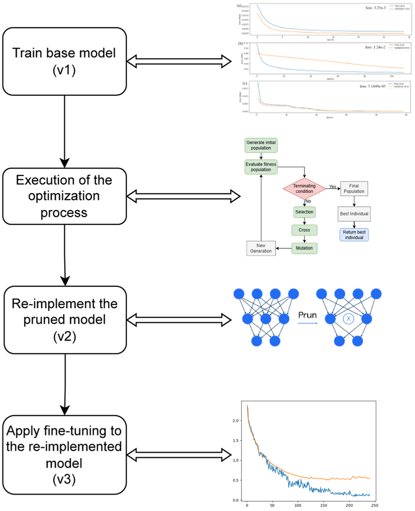
General scheme of the proposed technique.
Pruning using metaheuristics
Selecting the optimal subset of weights, filters, or neurons to eliminate in the context of neural network pruning can be described as a combinatorial optimization problem. The proposed technique is described as a local structured pruning method, which means that it targets the pruning of entire neurons from a particular layer (rather than considering the entire network). Therefore, the selection of the pruned input network layer is an important parameter for this new technique. When working with AE neural networks, the choice of which layer to prune is critical, as it can significantly affect the reconstruction capability of the model.
Metaheuristic parameters introduced
A set of additional parameters is introduced in addition to the classical metaheuristic parameters to ensure that the proposed method has a parameterized design and can be easily adapted to different situations and problems (as explained in the section “Metaheuristic parameters”). The parameters are as follows:
Maximum percentage of equivalent fitness: The maximum allowed percentage of the population that can share an equivalent fitness value. This parameter influences the stopping criterion, allowing the metaheuristic to terminate early if it becomes stuck in a local optimum and predominantly generates solutions with the same fitness.
Layer to prune: This specifies which input network layer will be pruned. The pruned layer size determines the individual size (i.e., the number of genes).
Proportion: In the context of pruning a neural network, the goal is to lose as little performance (or the relevant performance metric) as possible. Theoretically, the best performance could be achieved by keeping all neurons active. The maximum proportion of neurons that can remain active to prevent convergence toward trivial solutions is defined by this parameter.
Initial population generation
To generate the initial population,
Fitness evaluation
The definition of the optimal fitness function is one of the most delicate steps in implementing a metaheuristic for a specific problem. This is because the quality of the solutions in the population will be measured based on the selected fitness function, making defining a fitness function that reliably represents the quality of the solution crucial. In this particular case, the quality of an individual is determined by the ability of the network (after pruning the neurons indicated by the individual) to reconstruct a set of vibration signals (Figure 5). Specifically, the genetic information of the individual is used to determine which neurons in the “layer_to_mask” are deactivated. A set of vibration signals is then fed into the network for reconstruction, and the reconstruction loss is measured. This loss value is used as the fitness value: the objective is to minimize it (lower loss values indicate better reconstruction performance).
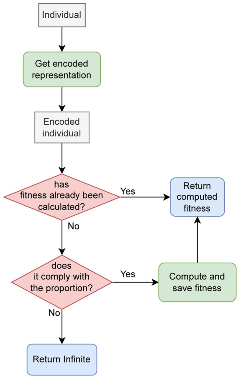
Fitness computation process with a memoization component.
The choice of reconstruction loss as the fitness function is motivated by the fact that it directly measures the property that must be preserved after pruning: the network’s ability to accurately reconstruct vibration signals from healthy structural conditions. Alternative criteria, such as weight magnitude or activation-based metrics, would provide only indirect approximations of post-pruning performance and might not reliably reflect the actual impact of neuron removal on reconstruction quality. By contrast, computing the reconstruction loss over a representative validation set ensures that each candidate solution is assessed based on the network’s end-to-end behavior, providing a more faithful measure of the pruning configuration’s quality.
Before proceeding with signal reconstruction, the current proportion of active neurons for the individual is evaluated to ensure that the restriction on the maximum number of active neurons is respected. If this proportion exceeds the “proportion” parameter, the individual is assigned a fitness value that indicates poor quality. Since the objective is minimization, a higher fitness value implies a worse solution, making it less likely that that solution will survive to the next generation. It is important to assign a sufficiently high penalty value to almost completely avoid considering solutions that violate the active neuron constraint.
An important point to highlight is that the selected fitness function is computationally expensive. Therefore, it is desirable to avoid the evaluation of the fitness function for identical individuals (the search process to generate previously encountered individuals). A resource optimization technique known as Memoization is used. This technique consists of caching the output of a function for a given input, allowing the cached output to be returned instead of recalculating it if the same input appears again. Thus, the method maintains a mapping between each individual and its corresponding fitness value, and the map is consulted before proceeding with the reconstruction and loss computation. If the fitness for the individual is already available, it is immediately returned; otherwise, it is computed and stored for future use.
Finally, to save computational resources related to memory usage, each individual (represented as a binary vector of length n_genes) is encoded into its integer decimal representation. This is done because storing a list in memory is generally more expensive (as it occupies more space) than storing a single integer. Figure 6 illustrates the difference between these two approaches: in the left table, fitness values are stored for a set of individuals using the binary list representation. The same information is stored in the right table, but the integer encoded version of the individuals is used.
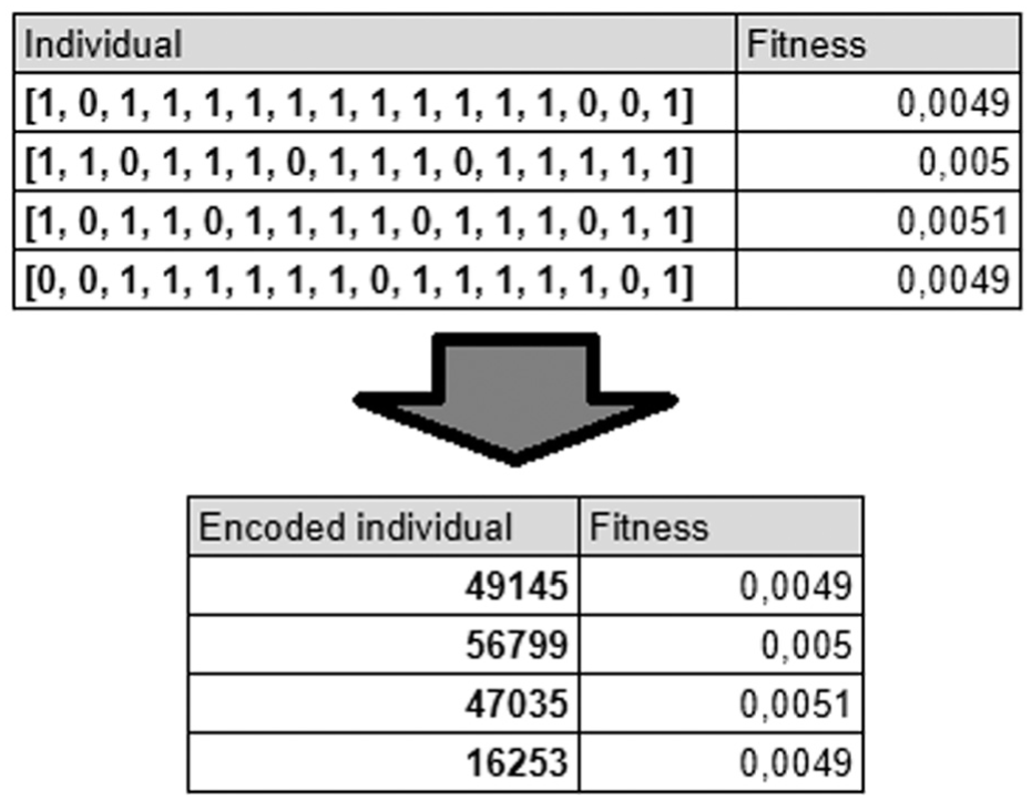
Process of encoding individuals to save memory.
Terminating criteria
The stopping criterion determines when the algorithm should stop generating new populations. In this particular technique, it depends on two main parameters. The number of generations created so far is compared with the parameter n_generations. If the current generation count is greater than or equal to this maximum, the algorithm terminates and returns the best solution found. An additional strategy known as early stopping is considered, which allows the algorithm to stop when it is detected to have converged. In this case, the number of individuals in the population with equivalent fitness is counted (different individuals may have the same fitness value), and the percentage of individuals sharing the most common fitness value is calculated over the entire population. If this percentage exceeds the value set by the Maximum percentage of the equivalent fitness parameter, the best solution is returned.
Genetic algorithm operators
The selection of operators in a metaheuristic depends heavily on the problem’s context and the way a solution vector is encoded. Choosing the right operators plays a key role in the ability of the technique to converge to high-quality solutions. Regarding the three main operators of a GA, the following were selected to select which individuals move to the next generation and how they are modified:
Selection operator: The tournament was selected. This operator involves running several “tournaments” between randomly selected individuals. In each tournament, the winners are chosen based on their quality, and these individuals advance to the next generation.
Crossover operator: A one-point crossover was used. This involves the selection of a random index in the parents to split them into two segments (head and tail). Then, two offspring are created by combining the segments of both parents (child 1: head of parent 1 and tail of parent 2; child 2: head of parent 2 and tail of parent 1).
Mutation operator: Bit-flip mutation is commonly used for binary encoded solutions. This operator randomly selects certain genes within an individual and transforms their value (a 1 becomes 0 and a 0 becomes 1).
An important consideration regarding the scope of the proposed method is that, while the proposed technique is formulated as a local structured pruning method (targeting neurons within a specific layer) the fitness evaluation inherently captures the global interactions among the network’s weights. Specifically, when a candidate solution deactivates a set of neurons in the pruned layer, the fitness function performs a complete forward pass through the entire network and measures the reconstruction error at the output. Consequently, any downstream effect caused by removing neurons in one layer is reflected in the overall reconstruction loss, allowing the metaheuristic to implicitly account for inter-layer dependencies when selecting which neurons to prune. Extending this approach to a fully global pruning strategy, in which the metaheuristic simultaneously decides which neurons to prune across all layers, is an interesting research direction discussed in the section “Future Work.” Such an extension would substantially increase the dimensionality of the search space, as the number of possible pruning configurations grows combinatorially with the number of layers and neurons, requiring more advanced search strategies or decomposition techniques to remain computationally feasible.
Post-pruning steps
After the optimization process is completed, the best configuration found by the metaheuristic is represented by a binary mask that indicates which neurons should be turned off. However, applying a mask simply sets the output of selected neurons to zero during inference, effectively ignoring them but not truly removing them from the network structure. Consequently, no real memory savings are achieved. The model must be reimplemented to realize actual memory usage reductions to remove the deactivated structures. If the optimized layer originally had
It is worth noting that the necessity and impact of fine-tuning are closely related to the proportion of neurons pruned. When the pruning proportion is moderate (i.e., a relatively small percentage of neurons are removed), the network retains sufficient capacity to maintain its reconstruction performance, and the metaheuristic is more likely to find a deactivation configuration that preserves the model’s behavior without requiring further adjustment. In such cases, fine-tuning may have a negligible effect or may even be unnecessary. Conversely, as the pruning proportion becomes more aggressive (i.e., a larger percentage of neurons are removed), the network’s capacity is more severely reduced, and the remaining architecture may need to redistribute its learned representations to compensate for the removed components. In these scenarios, fine-tuning becomes essential to allow the network to adapt its weights to the new, more constrained topology. This relationship between pruning aggressiveness and fine-tuning necessity is empirically validated in the following section, where the performance of the re-implemented models is analyzed both before and after the fine-tuning process across different pruning proportions.
Experiments
The following section presents the case study used to validate the proposed pruning technique. Additionally, the structural damage detection model used for the pruning tests is described. Finally, the different experiments performed are detailed, and the results obtained from pruning neural networks using the proposed technique are analyzed and compared with the structured local pruning method.
Case study description
For this study, data were obtained from a real bridge in Switzerland, connecting Utzenstorf and Koppigen, which was in service from the early 1960s until the late 1980s. A comprehensive instrumentation system was installed 1 year before demolition to study the influence of different environmental variables on the vibration behavior and dynamics of the bridge under various structural health conditions. This was possible because the bridge was subjected to different structural damage patterns over a full month, providing data from both the undamaged and damaged states. This dataset is currently one of the most widely used datasets in the literature, mainly because of its high-quality vibration data and variety of damage types.
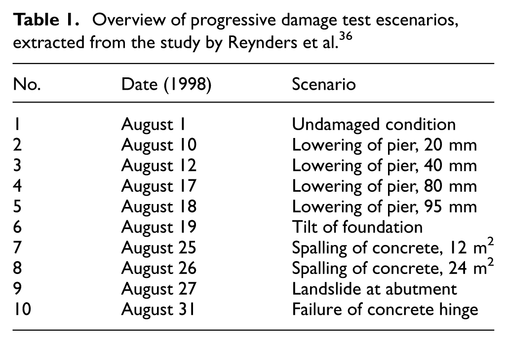
A complete instrumentation system, including sensors that measure atmospheric conditions and 16 sensors that record the bridge’s dynamic response (vibrations) was installed. Figure 7 shows some modifications made to the bridge to simulate different damage states, along with a side view of the bridge. Table 1 summarizes the complete history of all induced damage states and application dates. The dataset used in this study is publicly available and was originally introduced by Roeck et al. 8 It has been widely used as a benchmark in SHM research.
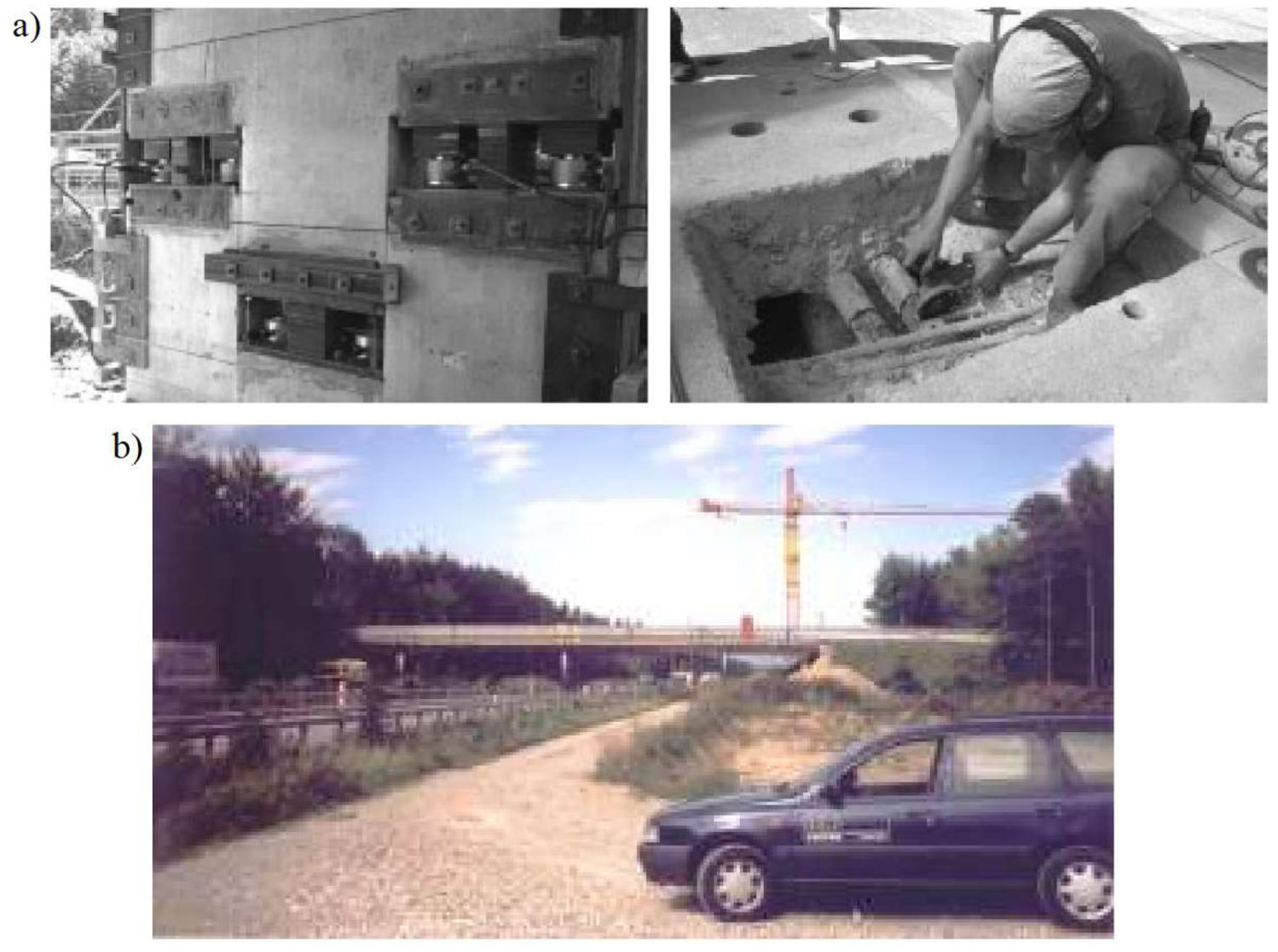
Overview of progressive damage test escenarios, extracted from the study by Reynders et al. 36
Damage detection model
As mentioned earlier, a damage detection model previously presented in the literature was used to validate this new technique, and its main components will be briefly described in this subsection. Figure 8 shows the complete damage detection framework comprising three main phases. A preprocessing step is applied to the vibration signals collected by the instrumentation system in the first phase. During preprocessing, the signals are divided into micro-sequences, and various techniques are applied to the ML model to condition the signals and facilitate their processing. The second phase involves training a neural network to learn to reconstruct only the signals corresponding to the bridge’s healthy state. In the third phase, a damage detection strategy based on thresholds is applied to determine whether a signal corresponds to a damaged or undamaged bridge state. This decision mainly relies on how difficult it is for the network to reconstruct the given signal. For a more detailed description of the damage detection framework used in this study, refer to the study by Santos-Vila et al. 37
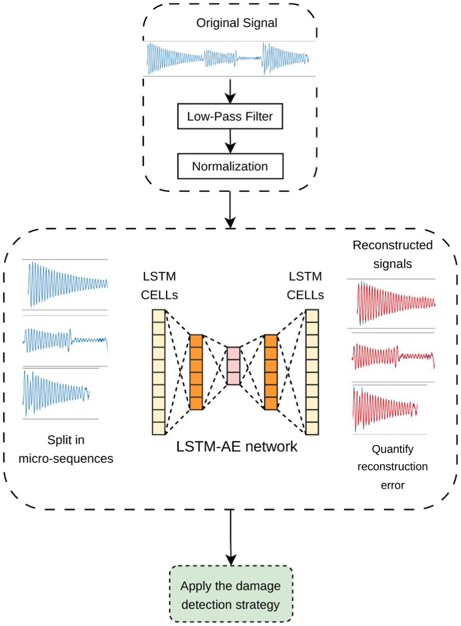
Damage detector model used in this study (extracted from the study by Santos-Vila et al. 37 ).
Although the original reconstruction model proposed in the referenced work was based on a long short-term memory (LSTM) network using an AE topology, the model in this study was simplified using only a feedforward AE (Figure 1). This simplification was made because LSTM networks have more complex internal connections, making deactivating certain components more challenging. Future research plans include extending this work to apply pruning techniques to the LSTM-AE network.
Defining the base models
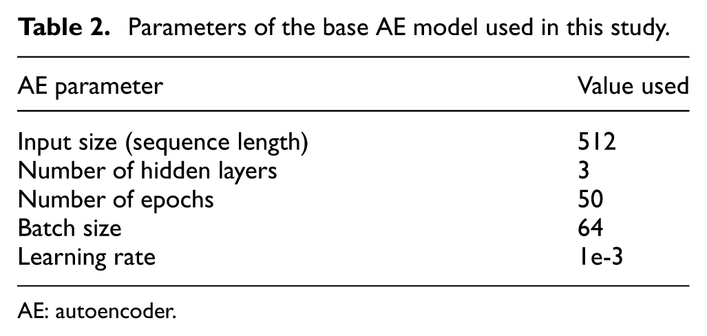
Before investigating the proposed technique’s pruning capabilities, a baseline must be established for comparison after pruning. This subsection presents the baseline model results (without pruning) used to verify that the model maintains good damage detection capabilities after pruning. Different neural network topologies were considered in this study to further enrich the experimental analysis. Table 2 lists some common parameters used across all models, and Table 3 summarizes all model variants considered for the experiments. This set of models mainly includes three models with the same number of layers but differing in the number of neurons per layer, ranging from 256 × 128 × 256 to 64 × 32 × 64. Additionally, each model was trained using a different training dataset, either monthly (covering all of March 1998) or weekly (covering the first week of March 1998), resulting in a total of six models (in all cases, the first week of April was used as the validation set). Furthermore, the table presents the main metrics used to evaluate the damage detection capability of the model, along with the minimum memory requirements to run each model, which will be used to highlight the memory reduction achieved after pruning.
Parameters of the base AE model used in this study.
AE: autoencoder.
Base models trained.
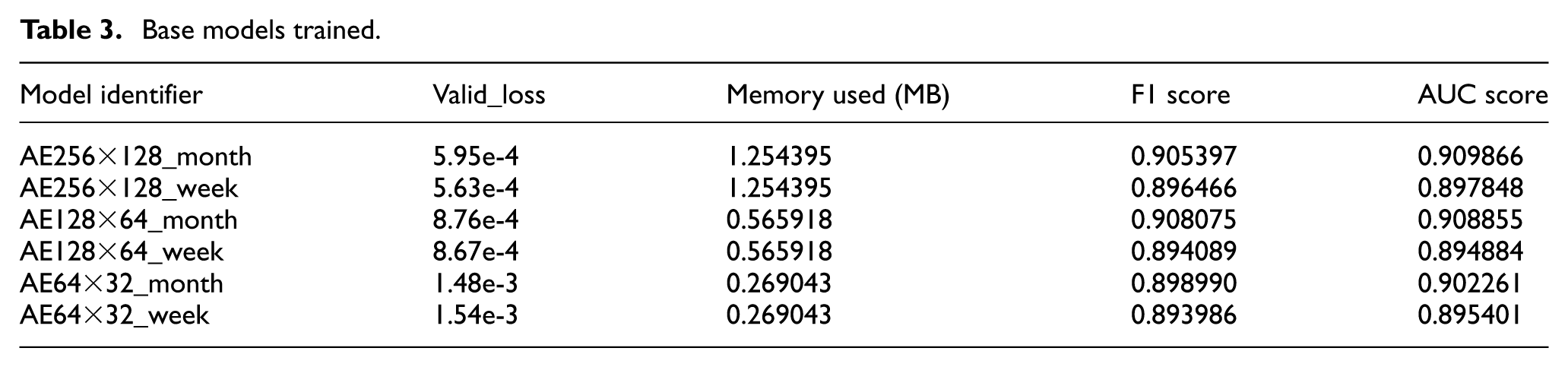
A set of signals from the bridge in both healthy and damaged states is used to test the model’s detection capabilities (which should ideally be preserved to some extent after the pruning process) to compute the F1 score 38 and AUC score 39 metrics. The signals measured between June 10 and June 25, 1998 were selected for the healthy bridge signal set. For the set of damaged bridge signals (with some type of structural damage), the signals measured between August 10 and August 25, 1998 were used.
Exploring pruning in different layers
The following subsection presents a set of experiments conducted to analyze how the performance of the AE model changes depending on which layer is pruned. As mentioned in the section “Autoencoders,” an AE is mainly composed of three layers: the encoder, bottleneck, and decoder. The parameters used to run the GA are shown in Table 4. The
Genetic algorithm parameters used in this study.
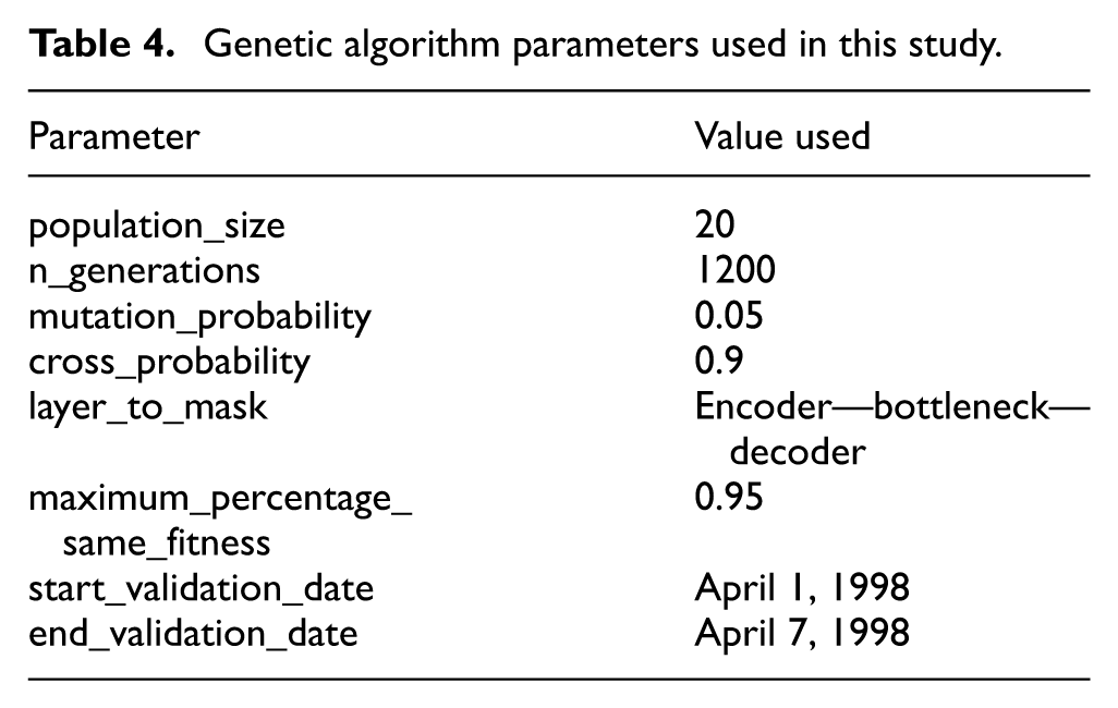
Figure 9 shows the results of pruning different layers of the network using both the classical structured local pruning technique and the proposed metaheuristic-based method, with the proportion parameter fixed at 0.7. For each technique, pruning was applied independently to the encoder, bottleneck, and decoder layers, yielding six experimental sets evaluated across the six model variants. Both techniques exhibit a consistent trend: pruning the decoder layer results in the lowest reconstruction error, closely followed by the encoder layer, whereas pruning the bottleneck layer leads to the worst performance across all configurations. This is expected, as the bottleneck layer has the lowest dimensionality, and removing neurons from it directly reduces the network’s representational capacity.
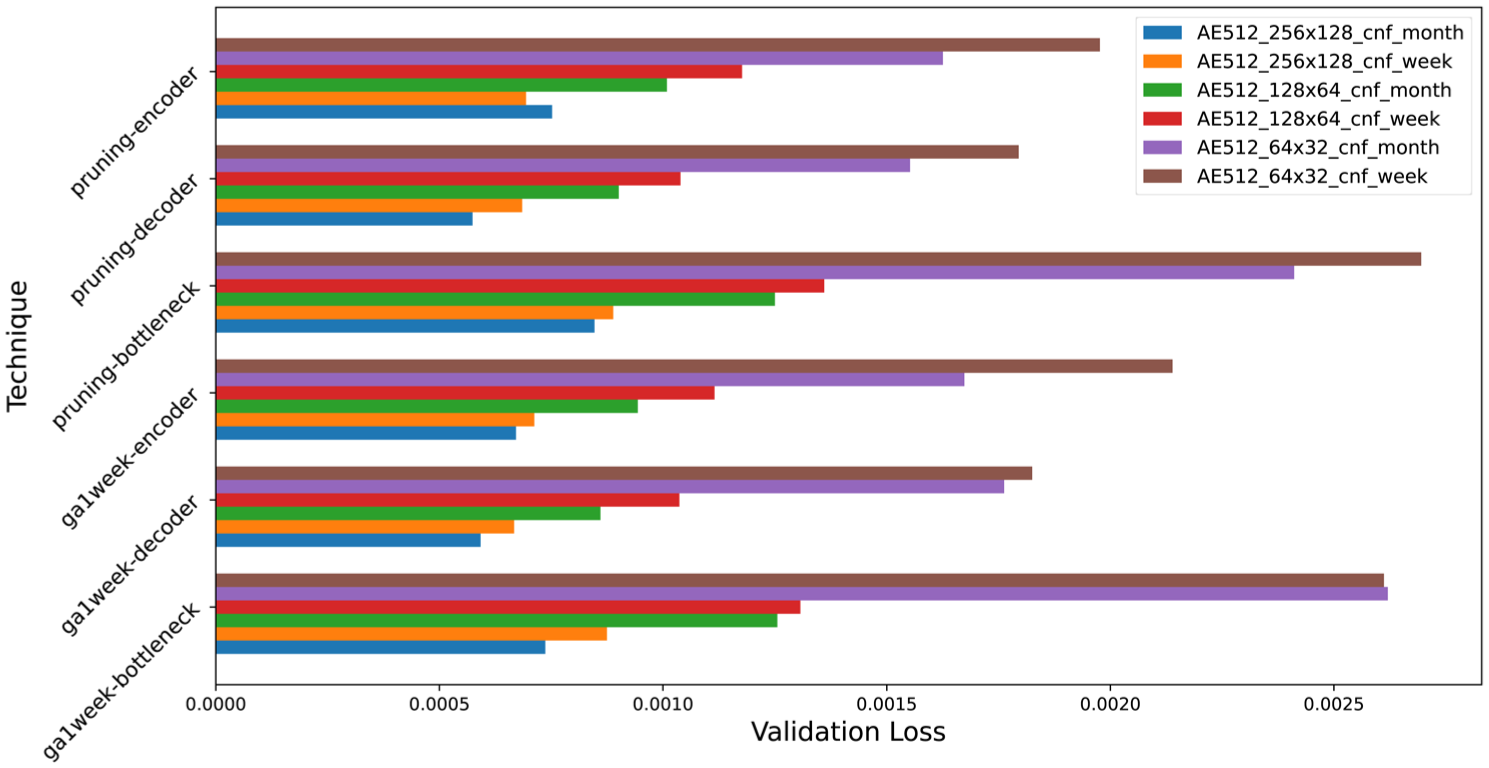
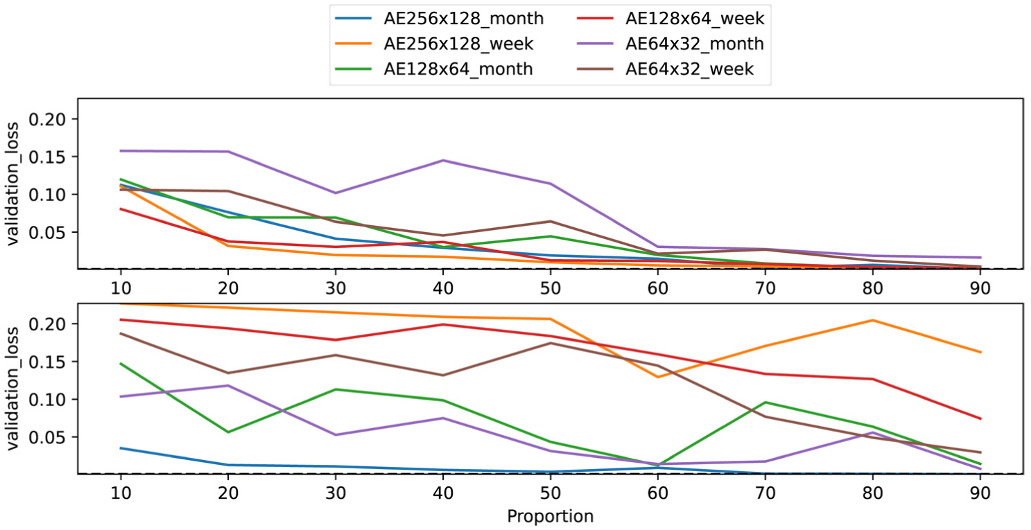
Validation loss for each model variation (after fine-tuning) considering different techniques and proportions.
Reducing the size of models
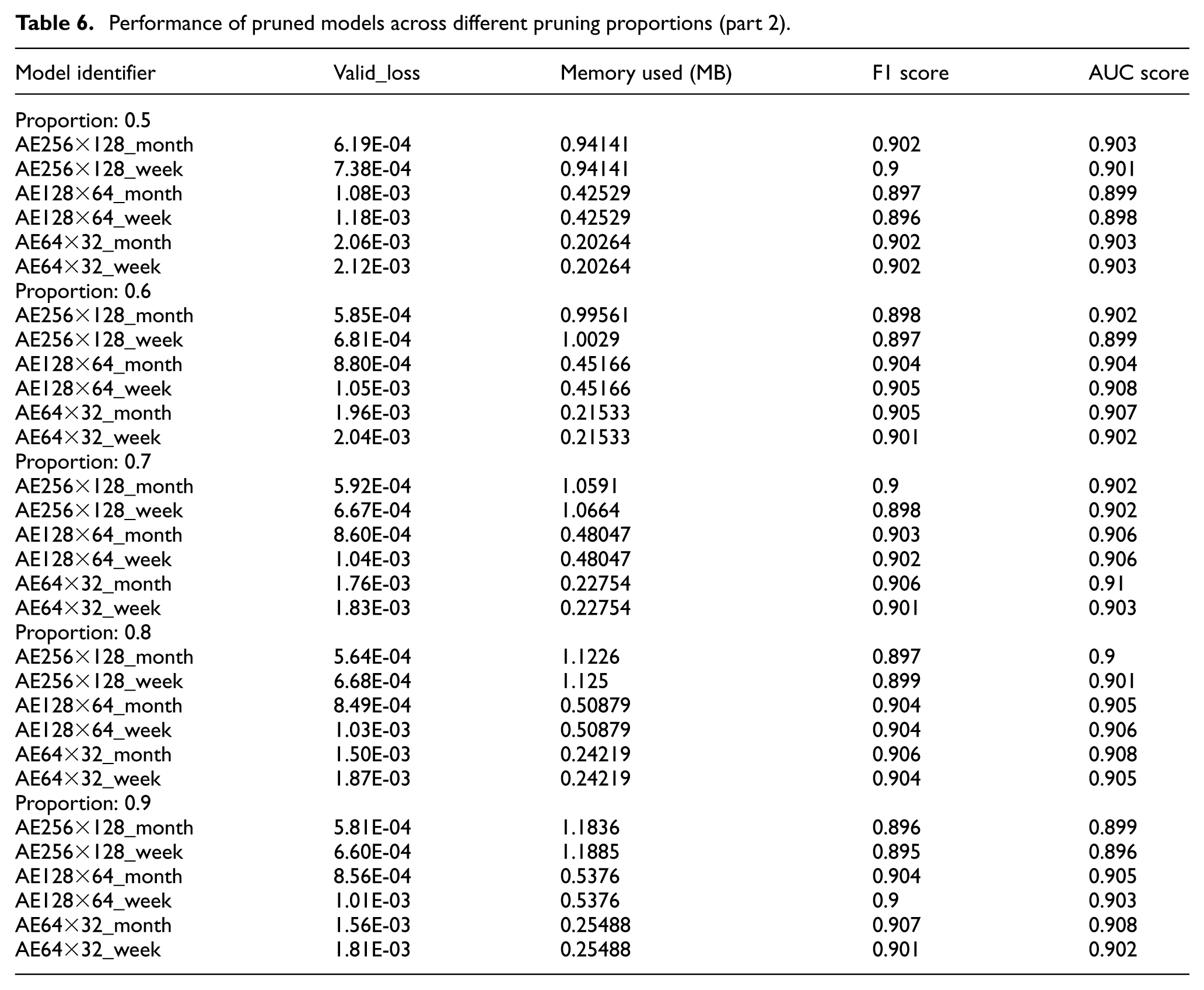
The following subsection analyzes how the model’s performance changes depending on the pruned number of neurons. Additionally, the proposed technique is compared with a classical pruning method to highlight the strengths and weaknesses of the approach. Structured local pruning was selected as the primary baseline because it is the most widely used approach for removing entire neurons from fully connected layers, making it the most directly comparable technique to the proposed method. For these experiments, the pruned layer was fixed as the decoder layer because the experiments in the section “Exploring pruning in different layers” showed that pruning this layer yielded the best results in terms of maintaining the network reconstruction performance after pruning. Furthermore, the parameter
Tables 5 and 6 present the experimental results, specifically the results obtained after the fine-tuning step was applied. These results show that the smaller the model, the greater the loss of accuracy as the parameter
Performance of pruned models across different pruning proportions (part 1).
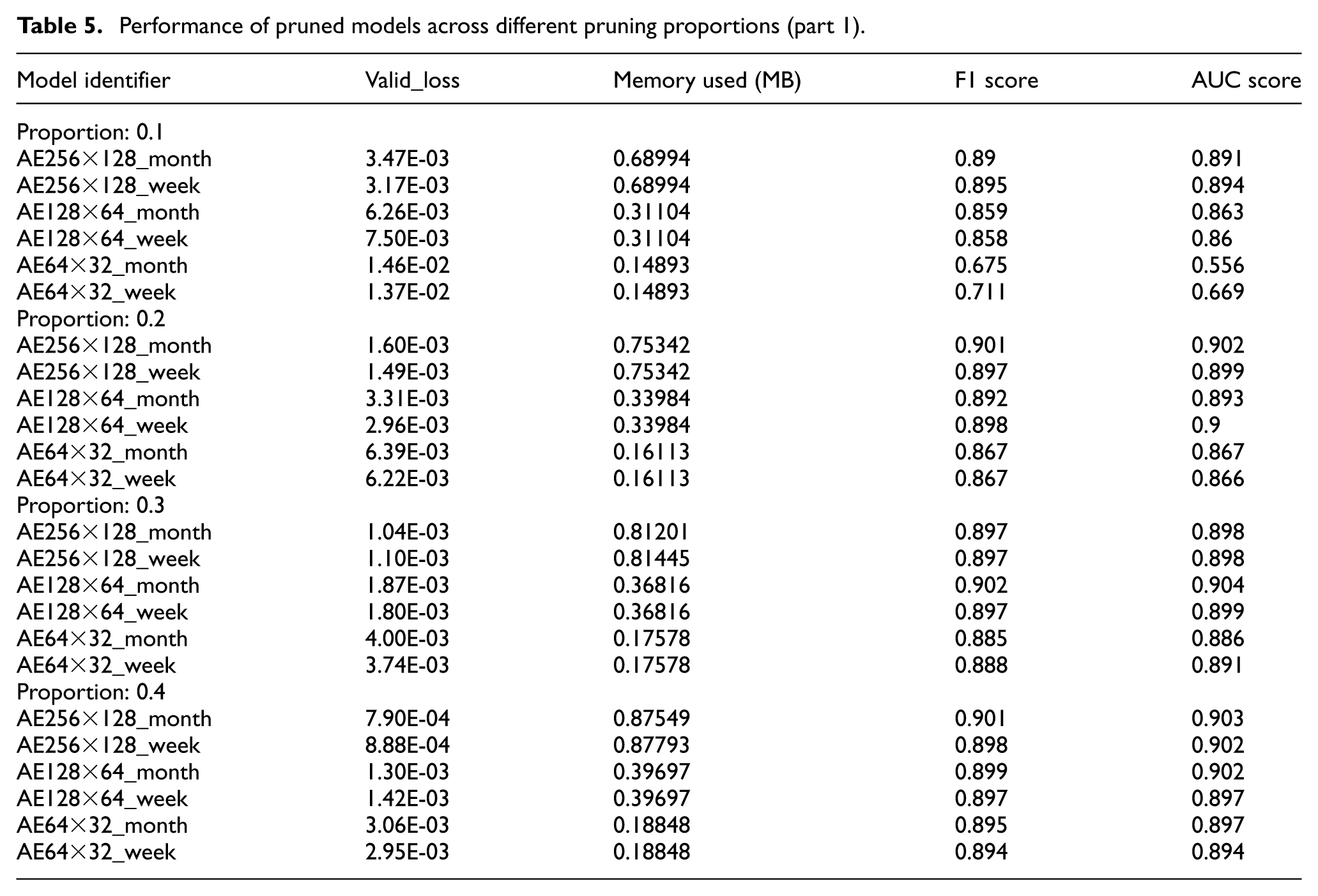
Performance of pruned models across different pruning proportions (part 2).
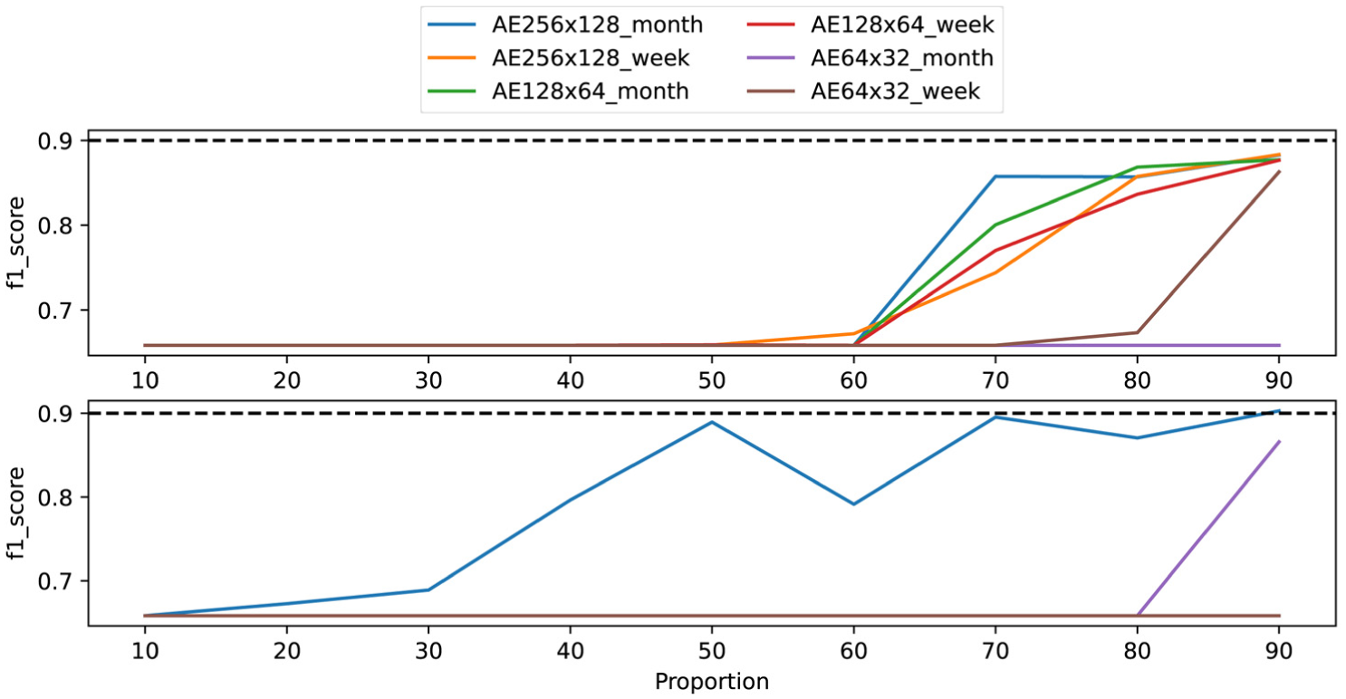
Figures 10 and 11 present a direct comparison between the proposed metaheuristic-based technique and the structured local pruning method, evaluating the re-implemented models before fine-tuning. This comparison is particularly informative, as it isolates the quality of the pruning decision itself, without allowing the model to recover through retraining. In terms of reconstruction quality (Figure 10), the proposed technique maintains a validation loss below 0.05 for most models down to a proportion of 40%, whereas structured local pruning exceeds this threshold from a proportion of 80%. This indicates that the metaheuristic identifies pruning configurations that preserve the network’s reconstruction capability under substantially more aggressive compression ratios. The contrast is even more pronounced for damage detection performance (Figure 11). Models pruned with structured local pruning lose nearly all ability to detect structural damage across most proportion values, with the majority of models collapsing to an F1 score around 0.65. In contrast, models pruned with the proposed technique retain meaningful detection capability down to a proportion of 70%. These results demonstrate that the metaheuristic-based approach produces fundamentally better pruning masks than the magnitude-based criterion used in structured local pruning, as the selected neuron configurations preserve both reconstruction accuracy and downstream damage detection performance even without fine-tuning.
Validation loss considering different values for
F1 score considering different values for
One of the strengths of this approach is that the model pruning phase using the metaheuristic technique can be performed on a different device than the one that will run the final, pruned model, which will be installed directly on the bridge. This way, the initial pruning phase is not subject to the same hardware limitations, and it is possible to leverage more powerful computational resources to execute the optimization process. The primary cost driver is the fitness evaluation, which requires a full forward pass of the validation set for each candidate solution in every generation. Although this represents a non-negligible one-time computational investment, it is important to note that the pruning process is performed offline and only once per model configuration. In contrast, the resulting pruned model (reduced by up to 45% in size) yields faster inference on every subsequent evaluation, an advantage that accumulates over the entire operational lifetime of the monitoring system, where continuous real-time assessments are performed. Therefore, the one-time optimization cost is largely offset by the long-term efficiency gains during deployment.
Statistical robustness
The following subsection briefly analyzes the performance of the proposed new method through 31 runs, focusing on verifying the consistency with which the model converges toward good solutions.
Figure 12 presents the convergence behavior of the proposed metaheuristic across multiple independent runs executed under identical parameter settings, aiming to assess the robustness and consistency of the optimization process. For visualization purposes, only 6 representative runs (out of a total of 31) are shown in the figure to improve readability and allow a clearer observation of individual convergence patterns. Each curve corresponds to a different run. As observed, the method progressively finds better solutions as generations evolve, consistently reaching fitness values in the range of 0.015–0.01 across all runs. Furthermore, the graph shows that the algorithm did not reach generation 1200 in some executions (e.g., green and orange curves), indicating that the stopping condition was triggered by the “Maximum percentage of equivalent fitness” criterion rather than the maximum number of generations.
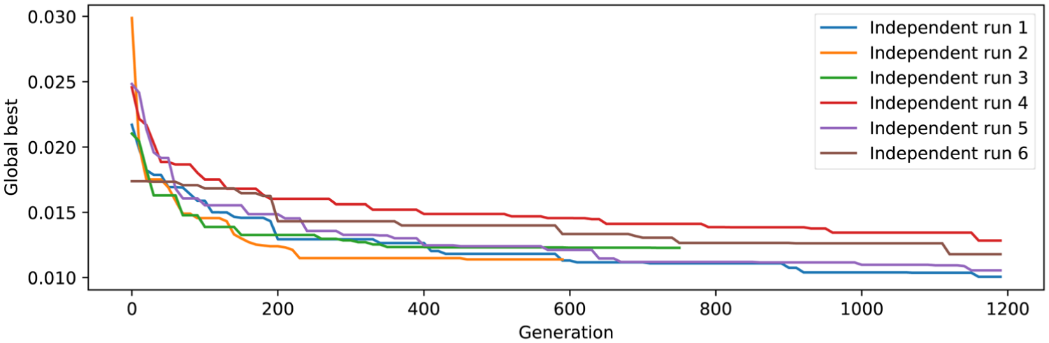
Convergence of metaheuristics considering different executions.
To assess the robustness of the proposed metaheuristic optimization process, an aggregated convergence analysis was conducted over 31 independent runs executed under identical parameter settings. For each generation, the mean and standard deviation of the validation error were computed across all runs. Figure 13 presents the resulting convergence curve, where the solid line represents the mean validation error and the shaded region indicates ±1 standard deviation. This visualization shows that the algorithm consistently converges toward similar solutions regardless of the initial random population. Moreover, the relatively narrow dispersion band observed throughout the optimization process indicates low variability between runs, supporting the stability and robustness of the proposed pruning strategy.
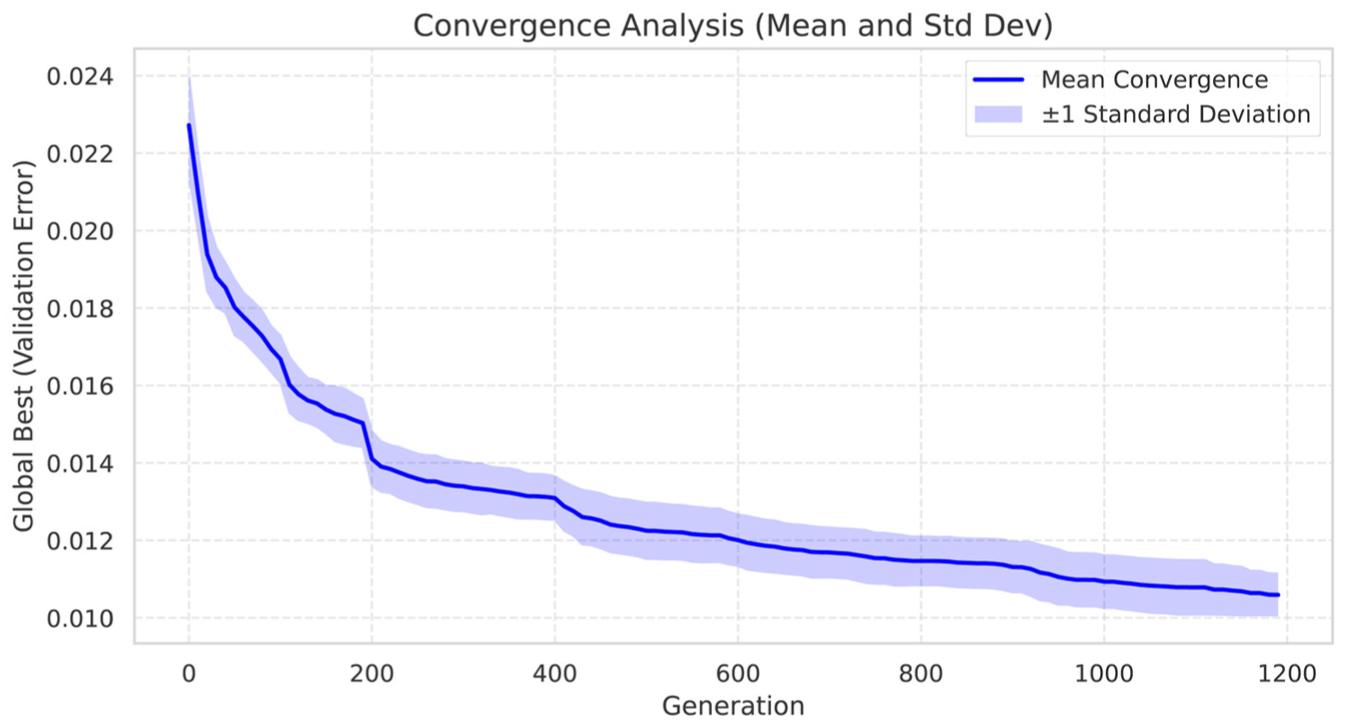
Aggregated convergence behavior of the proposed metaheuristic over 31 independent runs. The solid line represents the mean validation error across generations, while the shaded region indicates ± 1 standard deviation.
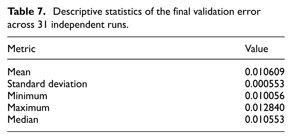
In addition to the convergence behavior, the final solutions obtained from the 31 runs were analyzed using descriptive statistics. Table 7 summarizes the distribution of the final validation error, including the mean, standard deviation, minimum, maximum, and median values. The results show a mean validation error of approximately 0.0106 with a very low standard deviation (0.00055), indicating that the optimization process consistently identifies solutions of similar quality. The small gap between the minimum and maximum values further reinforces the reliability of the approach. These results provide quantitative evidence that the proposed method yields stable and reproducible outcomes across multiple executions.
Descriptive statistics of the final validation error across 31 independent runs.
Beyond the quality of the final solutions, the consistency of convergence speed was also analyzed. Across the 31 independent runs, the metaheuristic algorithm was observed to reach a near-optimal solution within a relatively small number of generations. In particular, most runs achieved approximately 90% of their final fitness value within the early stages of the optimization process, indicating a rapid convergence behavior. This characteristic is particularly relevant from a practical perspective, as it suggests that the computational cost of the optimization phase can be controlled without significantly affecting the quality of the obtained solutions. This observation complements the discussion on the trade-off between optimization cost and deployment efficiency presented in the previous subsection.
The influence of the key parameters on the convergence and robustness of the proposed method was analyzed based on the experimental results. Regarding the pruning proportion, Figures 10 and 11 demonstrate that this parameter directly controls the trade-off between model compression and performance: the proposed technique maintains acceptable reconstruction quality down to a proportion of 40%, beyond which performance degradation becomes more pronounced. This provides practitioners with a clear guideline for selecting an appropriate compression level based on their specific performance requirements. Concerning the number of generations, an analysis of the 31 independent convergence runs reveals that the GA reached 90% of its final fitness value within a median of 710 generations, with most runs exhibiting minimal improvement beyond generation 310. This suggests that the budget of 1200 generations is sufficient to ensure convergence, while also indicating that fewer generations could be used in scenarios where computational resources are more constrained, with a modest impact on solution quality. The population size of 20 was selected to balance exploration capacity and computational cost. Each individual in the population requires a complete forward pass through the network over the validation set for fitness evaluation, making the per-generation cost proportional to the population size. A larger population would improve the diversity of candidate solutions and reduce the risk of premature convergence to local optima, but at a proportionally higher computational expense. The chosen value of 20 proved effective across all tested configurations, as evidenced by the low variance observed across the 31 independent runs (Figure 13), suggesting that the search space is adequately explored at this population size.
Conclusion
As previously discussed, certain instrumentation systems deploy processing nodes (small computational units) to reduce the data transmission cost. One of the challenges of this approach is that these devices often have limited hardware capabilities. Therefore, applying pruning techniques to ML models designed for structural damage detection could enable the direct deployment of such models directly on these nodes, enabling the implementation of more advanced solutions in resource-constrained environments.
A novel pruning technique based on optimization methods was proposed and validated in this study using a real-world case study. The results demonstrate the capability of the method to identify effective neuron configurations to prune, significantly reducing the size of the model while maintaining its performance. One of the key contributions of this study is that the proposed technique outperforms a well-known pruning method, structured local pruning, in several scenarios. The experimental results show that the proposed approach can reduce the size of the model by up to 45% while incurring only minimal performance losses. Moreover, the technique serves as a promising alternative to current pruning methods, offering greater flexibility and parameterization potential than some traditional approaches.
Regarding generalizability to different structures, the proposed pruning technique operates on the trained ML model independently of the specific structure being monitored. Since the metaheuristic optimizes which neurons to deactivate based on the network’s reconstruction performance, the method is in principle applicable to AE models trained on data from other bridges or civil structures, provided that a suitable baseline model has been trained. Certain aspects, such as the AE topology, input dimensionality (which depends on the number of sensors and signal characteristics), and GA parameters, may require minor adjustment depending on the specific monitoring scenario. With respect to generalizability across different neural network architectures, more significant modifications would likely be necessary. For example, applying this technique to recurrent architectures (such as LSTM-based networks) would require rethinking how neurons are deactivated, since these networks involve temporal dependencies and shared weight structures across time steps, making the effect of removing a single unit more complex to evaluate. Exploring the applicability of the proposed method to other architectures constitutes a promising direction for future research.
Future work
Owing to the limited attention that the scientific community has given to this type of technique, various research lines need to be explored. This subsection enumerates some of the most interesting ones that could help address some of the proposed technique’s underlying issues.
Selection of the validation set: The objective function used in this study can be considered costly in terms of execution time because the masked network must reconstruct the entire selected validation set to obtain the reconstruction error metric (which is used as the fitness value). If the validation set is relatively large, finding the best pruning mask will take more time. One way to address this problem is to use a smaller validation set. However, the evaluation of the network’s reconstruction ability after pruning certain neurons might lose significance because it would be assessed on a potentially non-representative subset of signals. Therefore, a potential research line would be to develop an intelligent selection method for a highly representative validation set while keeping its size reduced to avoid slowing down the pruning process.
Dynamic validation set: Another interesting research direction, also related to the validation set selection, would be to initially choose a subset for the early stages of the search process (where the metaheuristic is mainly exploring the search space). Then, the validation subset could be changed as stagnation in a local optimum is detected (requiring a recalculation of the fitness value for the current generation). This strategy could help escape local optima and allow the metaheuristic to explore the search space more extensively, potentially leading to better solutions.
Use of different types of metaheuristics: In this study, a genetic algorithm was used to search for neuron configurations that preserve the reconstruction performance of the network while allowing the deactivation of a minimal number of neurons. However, various metaheuristic techniques have been proposed, with new variants and algorithms being proposed each year. Selecting a subset of popular metaheuristics and conducting a comparative study to evaluate their performance would be very interesting. Such a study could provide deeper insight into why some techniques achieve better results than others.
Dynamic parameter adjustment: A fixed set of parameters was used across all experiments. Metaheuristics generally have an initial exploration phase (where diverse regions of the search space are examined) and an exploitation phase (where promising regions are intensively explored). The metaheuristic parameters (among other functions) determine when the technique is explored or exploited. Implementing a strategy that dynamically adjusts some metaheuristic parameters during the search process could be a potential improvement, thereby better guiding the search toward high-quality solutions.
Implementation of a global pruning technique: The proposed technique was designed to prune a specific network layer (thus falling into the local pruning category). However, modifying the technique to prune the entire network (transforming it into a global pruning technique) would be very promising. This would allow the metaheuristic to decide in which layers more neurons should be pruned and in which fewer neurons should be pruned, potentially achieving better results when the overall network size is reduced.
Footnotes
Funding
The authors disclosed receipt of the following financial support for the research, authorship, and/or publication of this article: This work was funded by the ANID/CONICYT + FONDEF Regular + Folio (ID24—10332) and partially supported by HPC OCÉANO (FONDEQUIP NoEQM170214).
Declaration of conflicting interests
The authors declared no potential conflicts of interest with respect to the research, authorship, and/or publication of this article.