






Abstract
Dam deformation prediction is a vital indicator for structural safety assessment. Although existing prediction models effectively extract temporal features from environmental variable sensor data, they inadequately capture the critical spatiotemporal coupling effects among hydraulic, thermal, and aging variables, which are primary influences on dam deformation behavior. To address this limitation, this study proposes a novel deep learning network named SAO-STformer, which integrates the Spatiotemporal-Transformer with the snow ablation optimizer. Specifically, the Spatiotemporal-Transformer model incorporates three significant enhancements over the traditional Transformer architecture. First, a multivariate patch embedding method is introduced to segment the sensor data of each variable into fixed-length temporal patches with positional encoding, forming a two-dimensional vector array that effectively preserves essential spatiotemporal information. Second, a spatiotemporal attention mechanism is implemented, consisting of: (1) a temporal attention layer that employs multihead self-attention to extract intravariable temporal dependencies and (2) a spatial attention layer incorporating a routing mechanism with dual multihead self-attention layers to establish comprehensive intervariable spatial connectivity. Third, a hierarchical scale fusion mechanism is introduced, whereby each encoder layer integrates adjacent variable patch representations to generate multiscale representations. Furthermore, the snow ablation optimizer is used for hyperparameter tuning of the Spatiotemporal-Transformer, and its dual-population mechanism helps balance global exploration and local exploitation, thereby reducing the risk of premature convergence and improving the reliability of the optimized model configuration. Upon validation using sensor data from a high arch dam, the proposed model outperforms traditional machine learning methods and existing Transformer variants across all evaluated metrics. The observed residuals, which are near zero and uniformly distributed, indicate an excellent model fit. Notably, the visualized spatiotemporal attention weights provide quantitative insights into the primary environmental variables and their dynamic coupling mechanisms that influence dam deformation. These findings offer significant theoretical contributions and practical guidance for dam safety monitoring and reinforcement strategies.
Keywords
Introduction
China has the largest number of high arch dams in the world. Since the completion of the 240-m-high Ertan Arch Dam in 2000, China has constructed several major high arch dams, including the Laxiwa, Xiaowan, Xiluodu, and Jinping I dams, which have significantly contributed to national strategies such as the Western Development and West-to-East Power Transmission projects. 1 Over its service life, a high arch dam is subjected to the combined effects of various internal and external factors, including construction conditions, environmental loads, and material properties. Consequently, the dam’s structural performance deteriorates over time, leading to frequent engineering defects and an increased risk of failure, thereby severely impacting the dam’s safe operation.2,3 High arch dams exceeding 200 m in height are subject to significant loads, posing greater challenges in areas such as crack prevention in large volumes of concrete, construction temperature control, and seismic safety.4,5 Furthermore, the large number and widespread distribution of safety monitoring sensors on high arch dams generate vast amounts of data on deformation, stress, and seepage, thereby making the timely and accurate analysis and evaluation of dam safety more challenging.6,7 Consequently, the focus in the field of dam engineering has shifted toward structural health monitoring. 8 Deformation serves as a comprehensive reflection of the structural state of concrete dams. 9 Developing robust models for analyzing and predicting deformation behavior is crucial for the real-time assessment of dam health and forecasting future operational behavior.
Deformations in concrete dams consist of reversible deformations induced by hydrostatic pressure and temperature changes, as well as irreversible deformations resulting from the nonlinear evolution of material and structural properties. 10 Consequently, dam deformation monitoring data are multivariate time series, comprising reservoir water level, temperature, and aging variables,11–13 which exhibit temporal, spatial, and spatiotemporal correlations. 14 To capture these time-varying characteristics, machine learning methods such as neural networks, 15 random forest (RF), 16 support vector machines (SVMs), 17 and extreme learning machines 18 have emerged as powerful tools for predicting dam deformation. While demonstrating strong generalization capabilities and prediction accuracy, 19 these models often struggle to accurately predict monitoring data with substantial fluctuations or complex lagged relationships, owing to their lack of recurrent connections.
To address these limitations, deep learning models such as long short-term memory (LSTM) networks 20 and gated recurrent units 21 have been applied to dam safety monitoring. These recurrent neural networks effectively capture nonlinear temporal patterns, thereby significantly improving deformation prediction accuracy. However, two critical limitations persist. One limitation is that the architecture requires strictly equal-length input and output sequences, which constrains variable-length prediction tasks for high arch dams. The other limitation is that vanishing and exploding gradient problems hinder the effective modeling of long-term dependencies beyond 100 time steps. 22 Correspondingly, two key innovations have been introduced. The encoder–decoder structure compresses the input sequence into a fixed-length vector, which the decoder subsequently uses to generate an output sequence of arbitrary length. 23 Attention mechanisms directly model dependencies across arbitrary time steps, thereby significantly enhancing the ability to capture long-range dependencies in time series.24–26 Vaswani et al. 27 proposed the Transformer model in 2017, which innovatively integrated these two approaches and completely eliminated the need for recurrence. Its core advantages are reflected in: (1) feature interaction: multihead self-attention (MSA) can automatically identify critical time points, such as sudden changes in reservoir water level and temperature, and assign higher attention weights to those points; (2) parallel processing: the self-attention mechanism allows the simultaneous processing of all time steps, improving training efficiency by five to eight times compared to that of LSTM; and (3) long-range dependency modeling: the theoretical receptive field covers entire sequences, reducing prediction error by 37% in precipitation forecasting tasks with more than 1000 time steps. However, the Transformer model exhibits significant shortcomings in predicting dam deformation, as it neglects the spatial correlation among adjacent monitoring sensors, thereby limiting its ability to accurately describe the overall deformation mode of the dam. 28
Furthermore, the prediction accuracy of deep learning models is heavily dependent on hyperparameter selection, which requires optimization algorithms to identify optimal configurations. In comparison to traditional mathematical optimization, metaheuristic algorithms offer distinct advantages, 29 such as gradient-free operation and structural simplicity. Metaheuristic algorithms are broadly categorized into two types: evolutionary algorithms 30 and swarm intelligence algorithms.31,32 Despite their diverse biological inspirations, all metaheuristic algorithms incorporate two essential phases: exploration and exploitation. The exploration phase globally searches the parameter space to identify promising regions for further investigation. The exploitation phase then locally refines solutions near the current optima. 33 However, most metaheuristic algorithms suffer from an exploration–exploitation imbalance, which significantly constrains their performance. The snow ablation optimizer (SAO) progresses through the snow-sublimation simulated exploration phase and the snow-melting simulated exploitation phase. Its dual-population mechanism dynamically balances the exploration–exploitation trade-off while preventing premature convergence. 34
In summary, the key to multivariate time-series prediction of dam deformation lies in combining historical information with the complex temporal, spatial, and spatiotemporal correlations among multiple environmental variables. Current research primarily focuses on temporal correlations, while neglecting spatial and spatiotemporal relationships, which limits improvements in prediction accuracy. Moreover, conventional hyperparameter optimization methods, such as particle swarm optimization (PSO), genetic algorithm (GA), and whale optimization algorithm, often fail to maintain an appropriate balance between exploration and exploitation in the solution space, leading to suboptimal parameter configurations. To address these limitations, the SAO-STformer network is proposed for predicting multivariate time series of dam deformation. The key contributions of this research are as follows:
The Transformer model is limited to extracting temporal features from environmental variable monitoring data. In contrast, the Spatiotemporal-Transformer model is capable of effectively retaining and extracting critical spatiotemporal features through the innovative use of multivariate patch embedding and the spatial–temporal attention mechanism, thereby enhancing the accuracy of dam deformation prediction.
The Spatiotemporal-Transformer introduces a scale fusion mechanism into the Transformer encoder–decoder structure. Each encoder layer combines adjacent environmental-variable patch representations to obtain representations at a coarser temporal scale, thereby improving the capture of both short-term fluctuations and long-term dependencies in the monitoring data and enhancing the accuracy of dam deformation prediction.
The SAO algorithm optimizes the Spatiotemporal-Transformer model’s hyperparameters by employing a dual-population mechanism. This mechanism balances global exploration with local exploitation, thereby avoiding premature convergence and enhancing the model’s performance and generalization.
The SAO-STformer demonstrates superior performance in dam deformation prediction compared with fourteen benchmark models. The visualized attention weights not only identify dominant environmental variables but also elucidate their dynamic coupling mechanisms that influence dam deformation, effectively addressing the interpretability challenges of black-box deep learning models.
The remainder of this paper is structured as follows. The second section presents the mathematical formulation for the multivariate time-series prediction of dam deformation. The third section provides a detailed description of the architecture of the proposed SAO-STformer network. The fourth section systematically evaluates SAO-STformer against fourteen benchmark models using monitoring data from a high arch dam. Ablation studies quantitatively demonstrate the contribution of each model component, while the visualized temporal and spatial attention weights provide physically interpretable insights into deformation mechanisms. The fifth section summarizes the main conclusions, discusses the limitations of SAO-STformer, and outlines future research directions.
Multipoint deformation prediction model of high arch dams
Concrete dam deformation consists of reversible deformations resulting from the cyclical effects of hydrostatic and thermal loads, as well as irreversible deformations due to time-varying effects, such as alkali-aggregate reactions, freeze-thaw cycles, and the development of joints and fissures, which may reduce the dam’s safety margin,
35
as shown in Figure 1. The hydrostatic-thermal-time (HTT) model is one of the most commonly used statistical models in the field of dam deformation monitoring. The theoretical basis of this model posits that the deformation of arch dams is primarily composed of three components: the water-pressure component

where
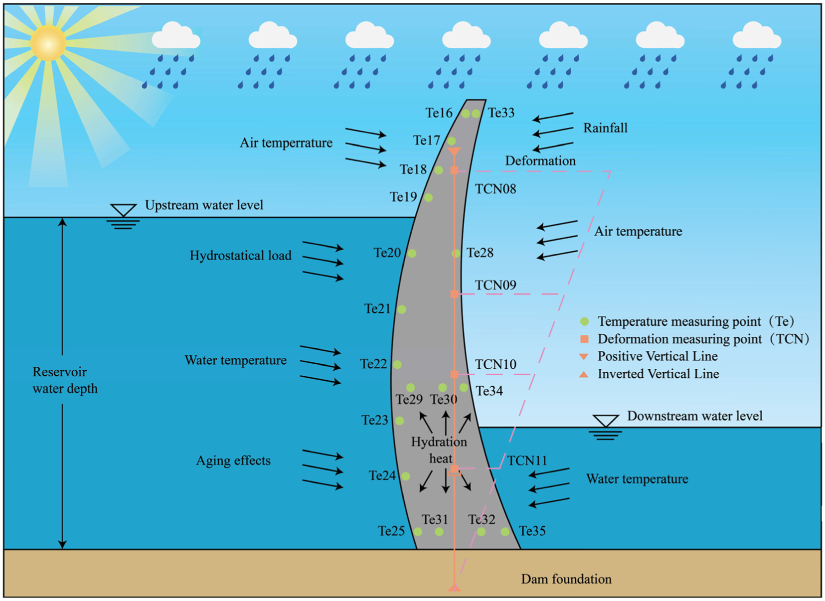
Mechanism of dam deformation.
Given the total number of time steps
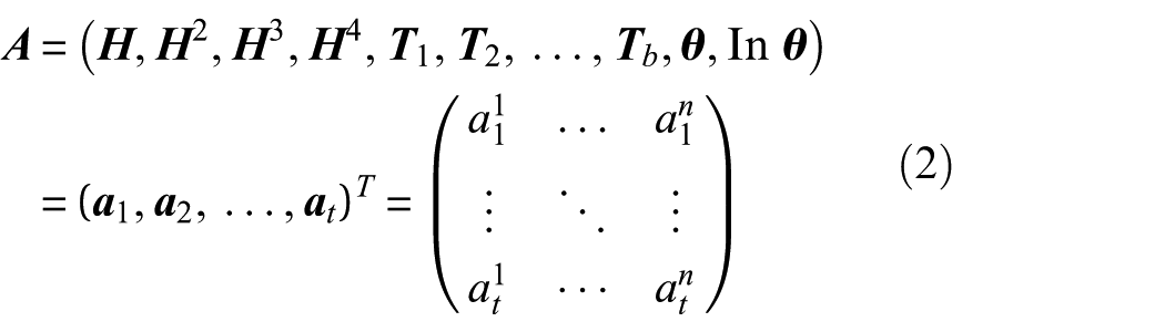
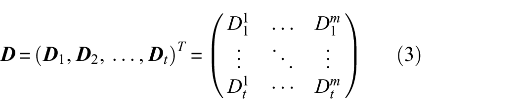
where
Similar to traditional HTT models, the proposed multipoint deformation prediction model first learns the mapping relationship between environmental variables and deformation responses from historical monitoring data. After this mapping is learned, the environmental-variable sequence in the target prediction period is used to predict the corresponding future deformation response. The main difference is that HTT models adopt a predefined statistical mapping function, whereas SAO-STformer learns a data-driven nonlinear spatiotemporal mapping

where
Methodology
Architecture of the SAO-STformer network
Figure 2 illustrates the overall architecture of the proposed SAO-STformer. The proposed architecture is designed to predict multipoint dam deformation by extracting spatiotemporal features and capturing both short- and long-term dependencies from multisource sensor monitoring data. The SAO-STformer consists of two main components: the Spatiotemporal-Transformer predictor and the SAO-based hyperparameter optimization module. In the Spatiotemporal-Transformer, multivariate patch embedding first segments the time series of each environmental variable into fixed-length temporal patches. Positional encoding is then incorporated to construct a two-dimensional vector array, thereby preserving key spatiotemporal information in the monitoring data before subsequent spatial–temporal attention modeling. The temporal attention layer captures intravariable temporal dependencies, whereas the routing-based spatial attention layer models intervariable spatial connectivity among environmental variables. The resulting spatiotemporal representations are then processed within a progressive encoder–decoder structure, where adjacent patch representations are progressively merged layer by layer in the encoder to construct multiscale temporal features. This design enables the model to integrate short-term fluctuations with long-term trends. Finally, SAO is used to optimize key hyperparameters of the Spatiotemporal-Transformer, thereby improving the stability and predictive accuracy of the model.
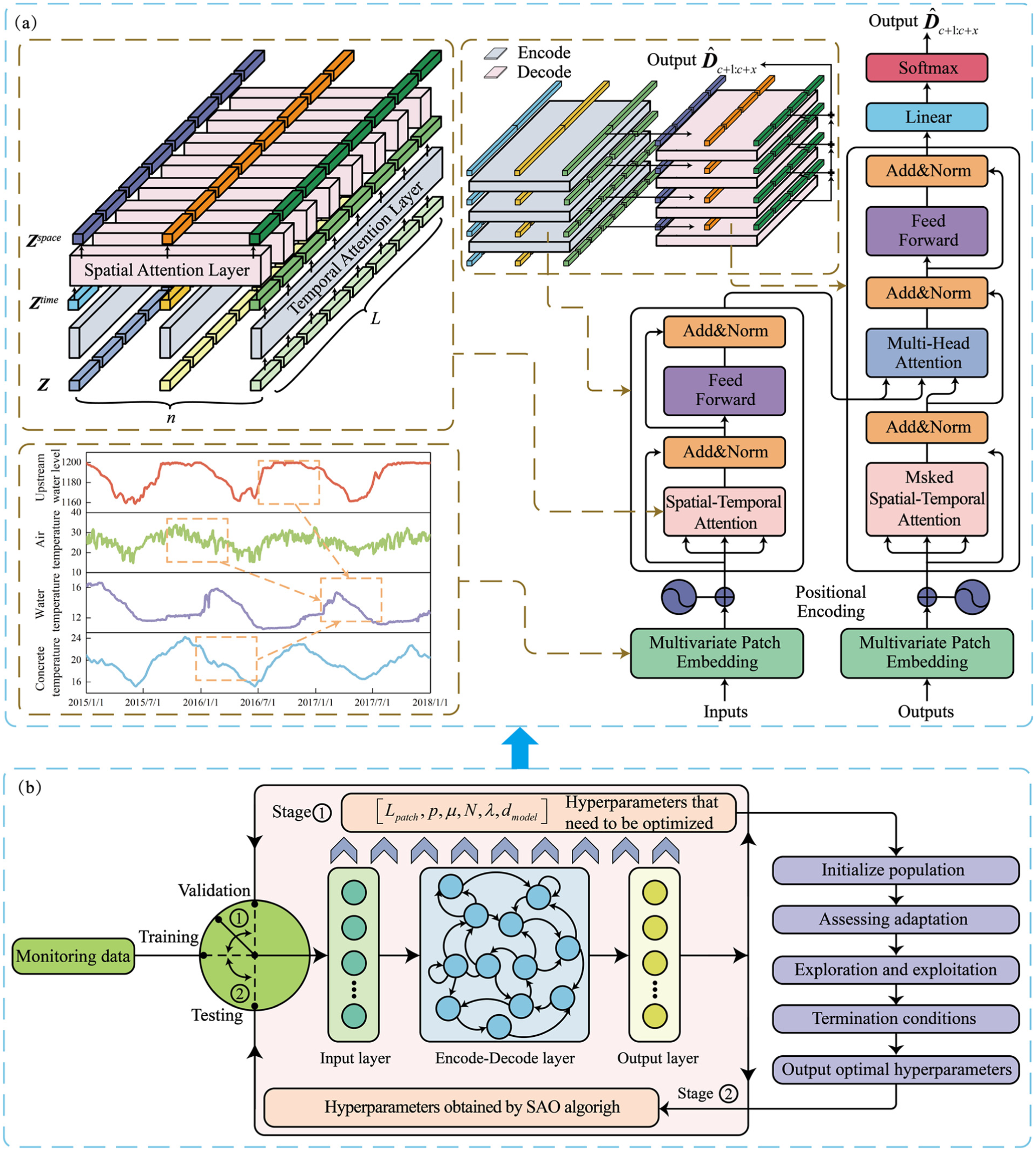
The framework of the SAO-STformer network: (a) Spatiotemporal-Transformer and (b) snow ablation optimizer. SAO: snow ablation optimizer.
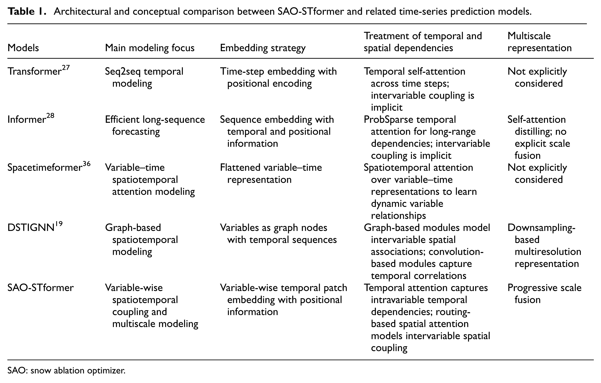
Table 1 further compares SAO-STformer with representative spatiotemporal time-series prediction models at the architectural and conceptual levels. Transformer 27 and Informer 28 mainly emphasize temporal dependency modeling, and intervariable spatial interactions are only implicitly represented. Spacetimeformer 36 explicitly considers variable–time relationships through spatiotemporal attention, while DSTIGNN 19 models spatiotemporal dependencies using graph-based spatial propagation and convolution-based temporal extraction. In contrast, SAO-STformer combines variable-wise patch representation, decoupled temporal attention and routing-based spatial attention, and progressive scale fusion. These differences clarify that the proposed model is not merely an application of existing spatiotemporal prediction architectures, but a task-oriented architectural extension for variable-wise spatiotemporal coupling and multiscale dependency modeling in dam monitoring data.
Architectural and conceptual comparison between SAO-STformer and related time-series prediction models.
SAO: snow ablation optimizer.
Spatiotemporal-Transformer
This section provides an overview of the architecture of the Transformer model, including key components such as input embedding, MSA, and the encoder–decoder structure. Building upon this foundation, three innovative improvements of the Spatiotemporal-Transformer model are introduced: the multivariate patch embedding, the spatial–temporal attention mechanism, and the progressive encoder–decoder structure.
Transformer
The Transformer is a deep learning model designed for sequence-to-sequence tasks. Its primary innovation is the introduction of the self-attention mechanism, which allocates varying attention weights to different sections of the input sequence to capture complex long-range dependencies within the data. Figure 3 illustrates the internal structure of the Transformer.
(1) Input embedding
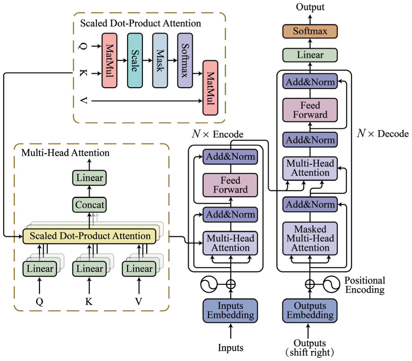
The internal structure of the Transformer.
The Transformer embeds the data of the

Positional encoding is achieved using sine and cosine functions of varying frequencies, which combine the vector

where
(2) MSA
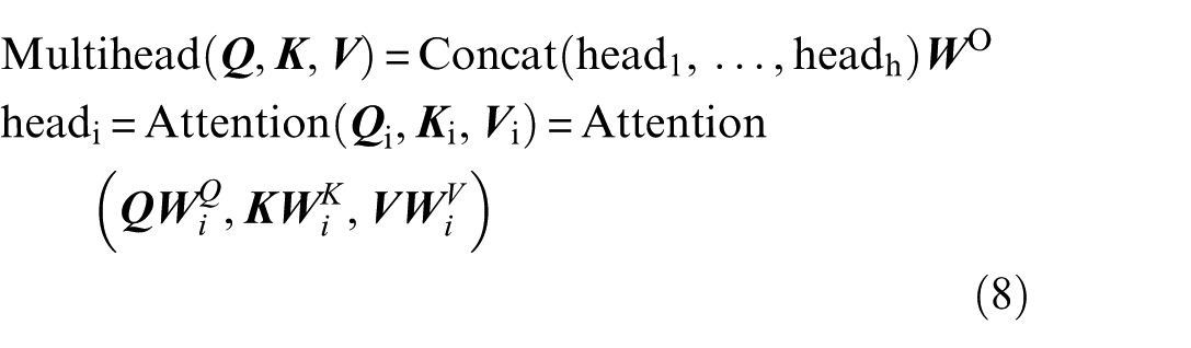
The MSA module comprises multiple scaled dot-product attention modules. Each scaled dot-product attention module generates three parameter matrices for learning: the query weights

where
The MSA module combines the outputs of each scaled dot-product attention module and applies a linear transformation to obtain the multihead attention values, as defined by the following formula:
where
(3) Encode–decode structure
As shown in Figure 3, the Transformer adopts an encoder–decoder structure. The encoder consists of N stacked layers, each containing an MSA sublayer and a feedforward sublayer, both followed by residual connections and normalization. The decoder also contains N stacked layers, with each layer comprising a masked MSA sublayer, an MSA sublayer connected to the encoder output, and a feedforward sublayer. The masked MSA prevents the decoder from attending to future positions, while the second MSA sublayer uses the decoder states as queries and the encoder outputs as keys and values, enabling the decoder to generate future deformation sequences based on the encoded environmental-variable monitoring information.
Multivariate patch embedding
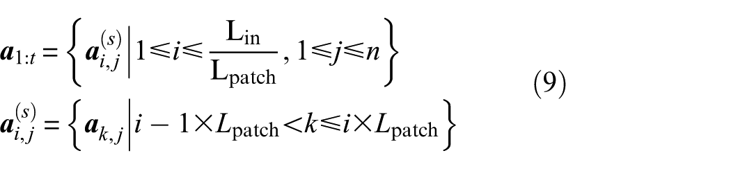
For dam monitoring data, different environmental variables, such as reservoir water level, temperature, and aging, have distinct temporal evolution patterns and physical meanings. As shown in Figure 4(a), the standard Transformer embeds data from different variables at the same time step into a single vector, which may obscure variable-specific temporal patterns. In addition, data from a single time step provide limited local temporal context. To address this limitation, multivariate patch embedding segments the time series of each environmental variable with length
where
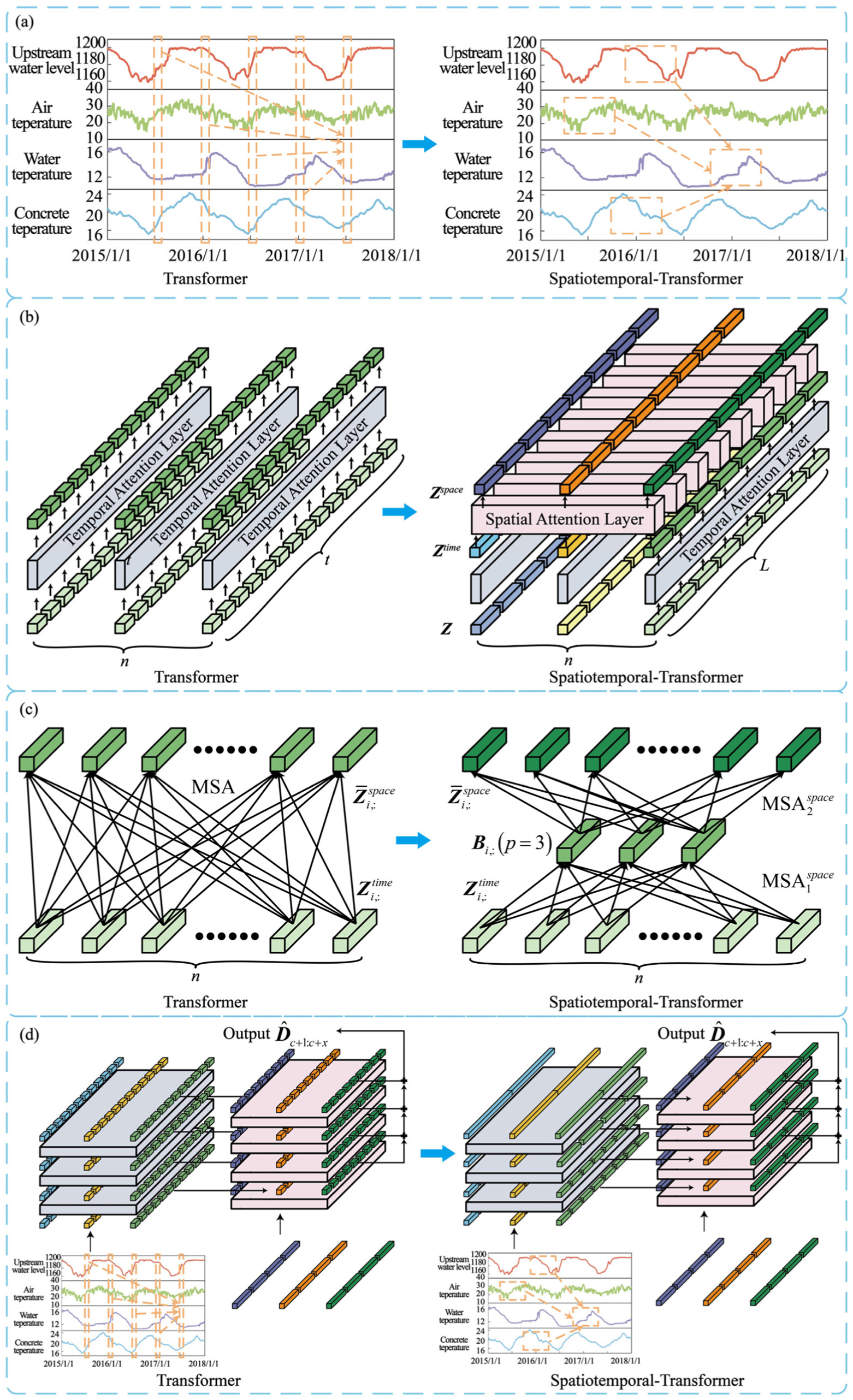
Comparison between Spatiotemporal-Transformer and Transformer architectures: (a) multivariate patch embedding, (b) spatial-temporal attention mechanism, (c) routing-based spatial attention, and (d) progressive encoder – decoder structure with scale fusion.
Each temporal patch is then linearly projected and combined with positional information

where
Spatial–temporal attention mechanism
As shown in Figure 4(b), the standard Transformer mainly relies on temporal self-attention and only implicitly captures the spatial dependencies among environmental variables. However, dam deformation is governed by the coupled effects of environmental variables, and neglecting these intervariable interactions may weaken the representation of deformation-driving mechanisms. To address this limitation, the Spatiotemporal-Transformer introduces a spatial–temporal attention mechanism with two layers: a temporal attention layer for capturing intravariable temporal dependencies and a routing-based spatial attention layer for modeling intervariable spatial dependencies.
(1) Temporal attention layer
Let the input to the temporal attention layer be


where
(2) Spatial attention layer
As shown in Figure 4(c), directly applying MSA to all variable pairs at each temporal patch would lead to a computational complexity of




where
The spatial–temporal attention module connects any two vectors from the input (i.e.,
Progressive encoder–decoder structure
Dam deformation is affected by both short-term environmental fluctuations and long-term operational trends. Short-term fluctuations may be caused by rapid changes in water level or temperature, whereas long-term trends are associated with seasonal variation and aging effects. To capture these different temporal scales, a progressive scale fusion mechanism is introduced in the encoder–decoder structure. By merging adjacent patch representations layer by layer, the model gradually constructs coarser temporal representations, enabling it to integrate local fluctuations and long-term trends.
As shown in Figure 4(d), in the encoder, each encoder layer except the first combines two adjacent patch representations to generate a representation at a coarser temporal scale:
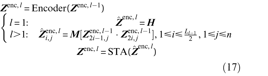
where
Let

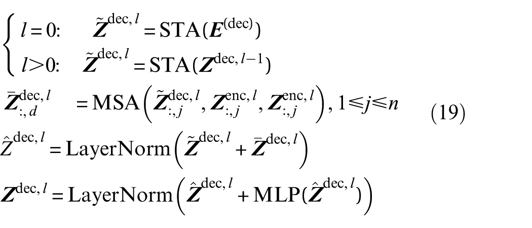
where
A linear projection is applied to the output of each layer to obtain the deformation prediction
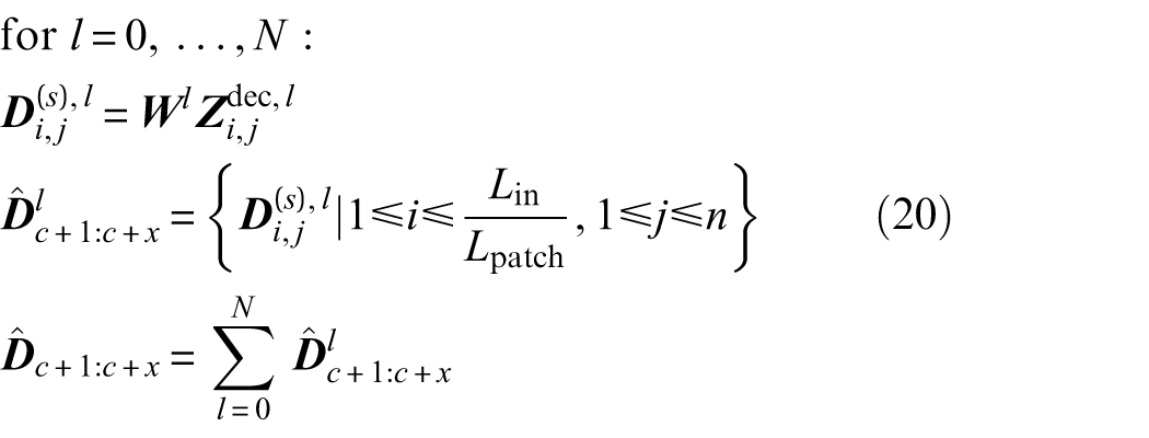
where
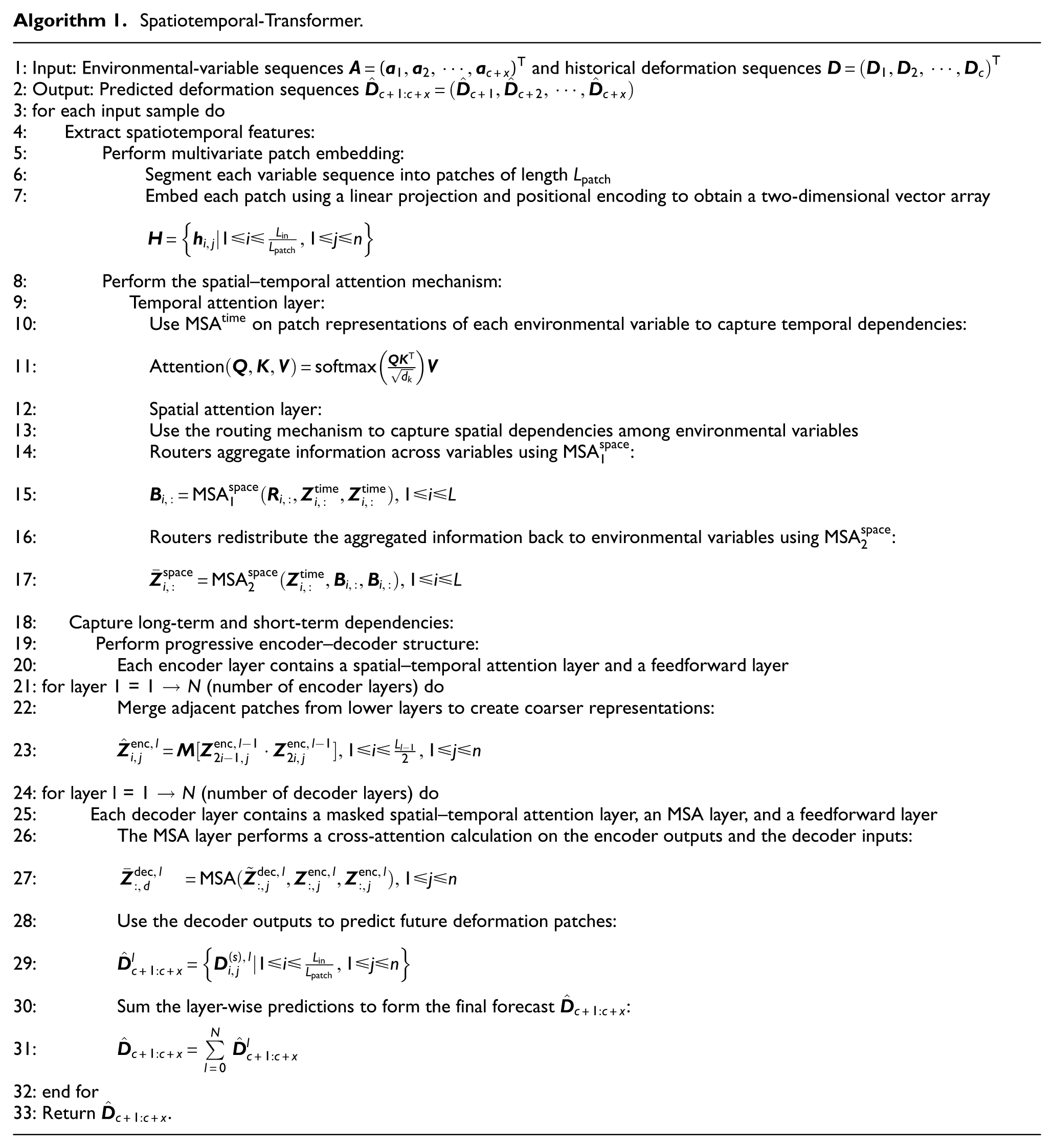
The algorithmic process of the Spatiotemporal-Transformer model is outlined in Algorithm 1.
Spatiotemporal-Transformer.
Snow ablation optimizer
To further enhance the performance of the Spatiotemporal-Transformer model in dam deformation prediction, it is crucial to optimize its hyperparameters. Traditional metaheuristic algorithms, such as GA and PSO, often suffer from premature convergence and struggle to maintain a balance between exploration and exploitation in the hyperparameter search space. The SAO simulates the processes of snow sublimation and melting, as illustrated in Figure 5(a). During sublimation, snow transitions into water vapor and disperses stochastically, promoting effective exploration of the search space. In contrast, the melting process converts snow into liquid water, representing an exploitation phase. By adopting a dual-population mechanism, the SAO algorithm effectively balances exploration and exploitation, enabling efficient optimization. 37 The flow of the SAO algorithm is depicted in Figure 5(c)–(f). The detailed processes are as follows:
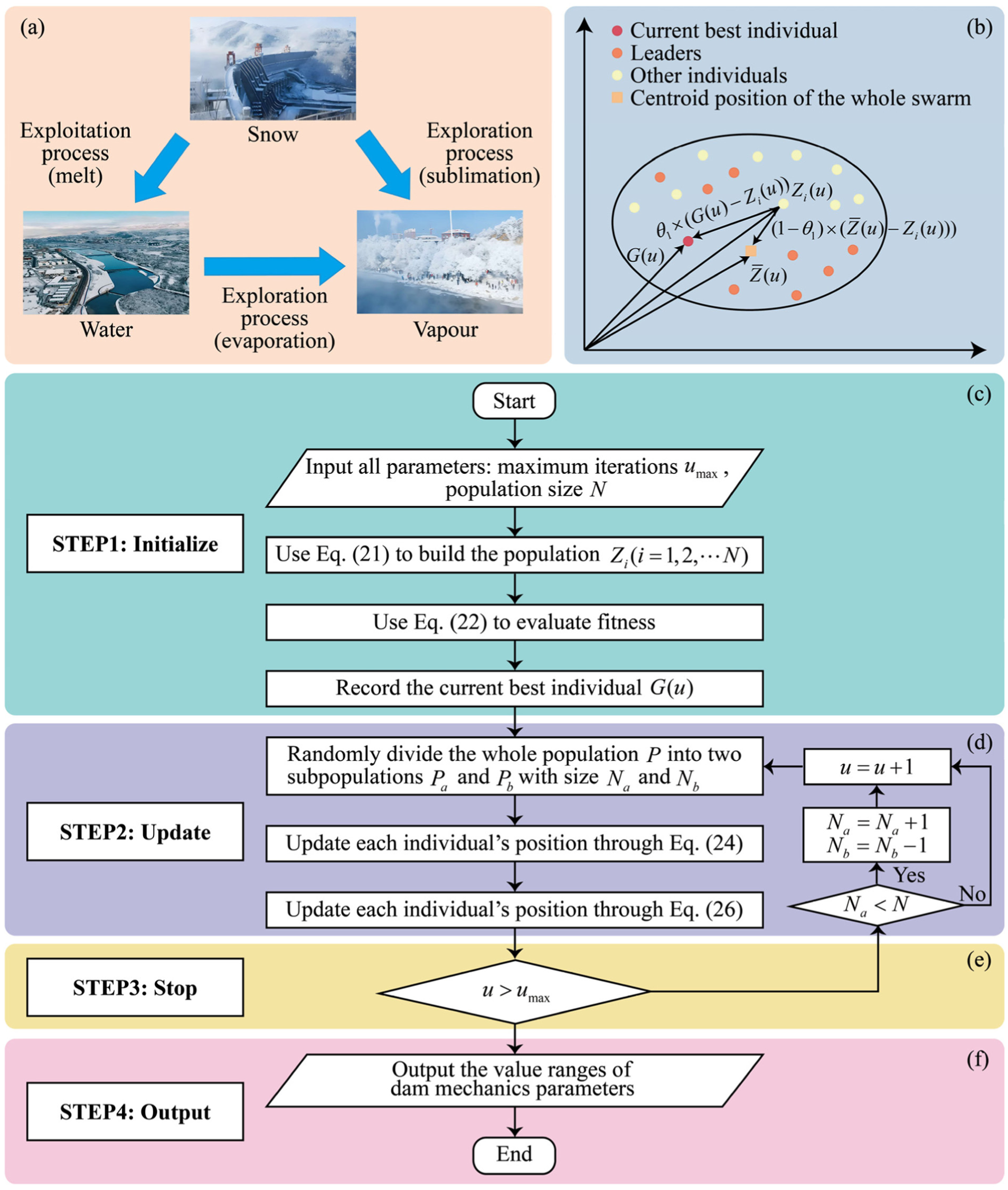
Flowchart of SAO. SAO: snow ablation optimizer: (a) snow-ablation-inspired exploration – exploitation mechanism, (b) position-update mechanism, (c) initialization and fitness evaluation, (d) dual-population update, (e) stopping criterion, and (f) output of the optimized hyperparameters.
In the initial phase, a set of randomly generated hyperparameter samples is modeled as a matrix
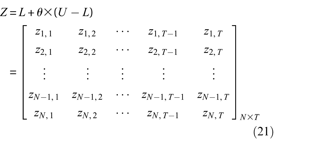
where
The overall coefficient of determination
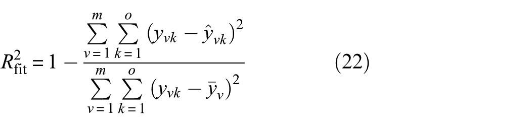
where
Exploration phase
During the exploration phase, Brownian motion is employed to model the stochastic behavior of water vapor within the parameter space

Figure 5(b) illustrates the position update using the following expression:
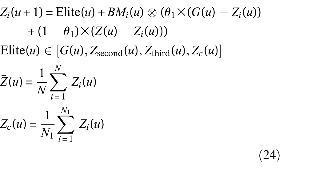
where
Exploitation phase
In the exploitation phase, the degree-day method 38 is employed to simulate the snowmelt process, with the following expression:

where
The position update equation is as follows:

where
Dual-population mechanism
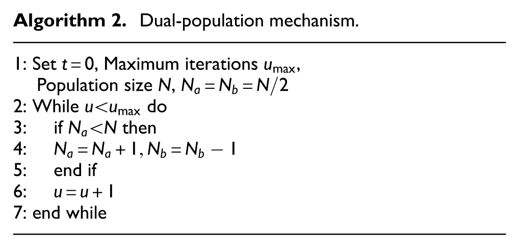
The dual-population mechanism is employed to balance exploration and exploitation, as shown in Algorithm 2. In the initial stages of the iteration, the entire population
Dual-population mechanism.
Case study
Description of the dam and monitoring data
The dam of a hydropower station is located on the mainstream of the Yalong River in Panzhihua City, Sichuan Province, China. The dam is a concrete parabolic double-curvature arch dam with a maximum height of 240 m and a top arc length of 774.69 m. It is divided into 39 dam segments. The dam primarily consists of flood discharge structures, energy dissipation structures, water conveyance structures, and underground powerhouses. The dam’s normal water level is 1200 m, with a total storage capacity of 5.8 billion cubic meters and an adjustable storage capacity of 3.37 billion cubic meters, allowing for seasonal regulation.
The dam’s safety monitoring system primarily includes temperature monitoring, reservoir water level monitoring, deformation monitoring, seepage monitoring, and stress–strain measurements. To monitor horizontal displacements at locations such as the crown, arch shoulders, and the 1/4 arch ring, eight inverted vertical lines and ten positive vertical lines were arranged within the dam, forming five sets of vertical lines, with a total of 20 deformation-monitoring points coded as TCN measurement points. The radial horizontal displacement is automatically observed and recorded once daily, facilitating the modeling and prediction of dam deformation. This study selects data from six typical measurement points (TCN03, TCN05, TCN08, TCN09, TCN15, and TCN16) in dam segments 11, 21, and 33 for analysis. Dam segments 11 and 33 are located on the riverbank, while dam segment 21 is situated in the middle of the river valley. Deformation at these three different locations exhibits distinct evolutionary patterns, providing a comprehensive reflection of the overall deformation characteristics of the dam. The arch dam shape and deformation-monitoring-point layout are shown in Figure 6.
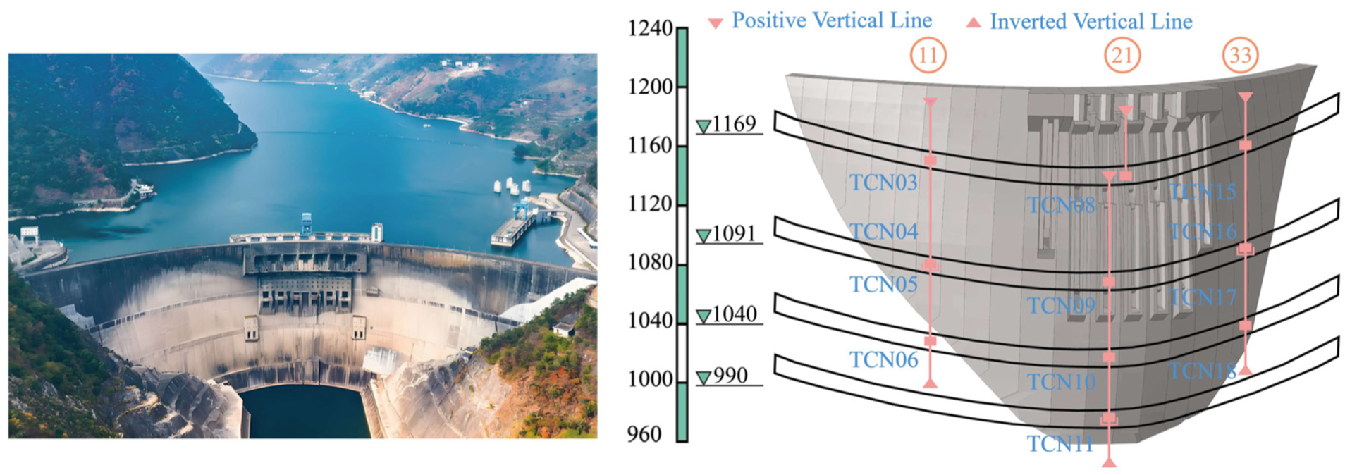
Arch dam shape and deformation-measurement-point layout.
Figure 7 illustrates the monitoring layout and time histories of dam deformation and environmental variables for sections 11, 21, and 33. As shown in Figure 7, temperature sensors were installed on the upstream face, downstream face, and inside the dam body of sections 11, 21, and 33 to measure water temperature, air temperature, and internal concrete temperature, respectively. These thermometers consist of vibrating-wire and semiconductor sensors, with a total of 44 units deployed. The figure also presents the radial horizontal displacement records of multiple monitoring points, together with reservoir water level, temperature, and rainfall data. The dataset for each monitoring point contains 2762 daily observations collected from January 1, 2008, to December 31, 2016, and was divided into training, validation, and test sets at a ratio of 6:2:2. To reduce the influence of different measurement scales, the data from all monitoring points were normalized before model training. The deformation responses of different dam sections exhibit clear periodic variations and show strong consistency with changes in reservoir water level and temperature. In general, larger deformation values occur during the cold season, particularly from October to January, when reservoir water levels are relatively high and the thermal contraction effect becomes more pronounced. By contrast, smaller deformation values are observed from April to June, when the reservoir water level is relatively low and the temperature field gradually increases. The maximum deformation values of sections 11, 21, and 33 are 64.23, 139.70, and 48.24 mm, respectively, and their corresponding maximum annual variation amplitudes are 39.73, 69.02, and 28.24 mm. These results indicate that the deformation response of the riverbed section is more sensitive to environmental changes than that of the bank sections. For Section 21, the maximum deformation values at TCN08, TCN09, TCN10, and TCN11, located at elevations of 1169.05, 1093.05, 1043.05, and 980.05 m, are 139.70, 125.25, 76.11, and 39.78 mm, respectively. The corresponding maximum annual variation amplitudes are 69.02, 78.87, 54.13, and 32.94 mm, respectively. Similar distribution patterns can also be observed in the other sections, suggesting that monitoring points at higher elevations generally exhibit stronger deformation responses to environmental variables. Overall, Figure 7 demonstrates a clear spatiotemporal correlation between dam deformation and environmental variables, which provides the physical basis for extracting spatiotemporal features in the proposed Spatiotemporal-Transformer model. In this study, 49 environmental variables, including reservoir water level, temperature, rainfall, and aging factors, were selected as model inputs

where
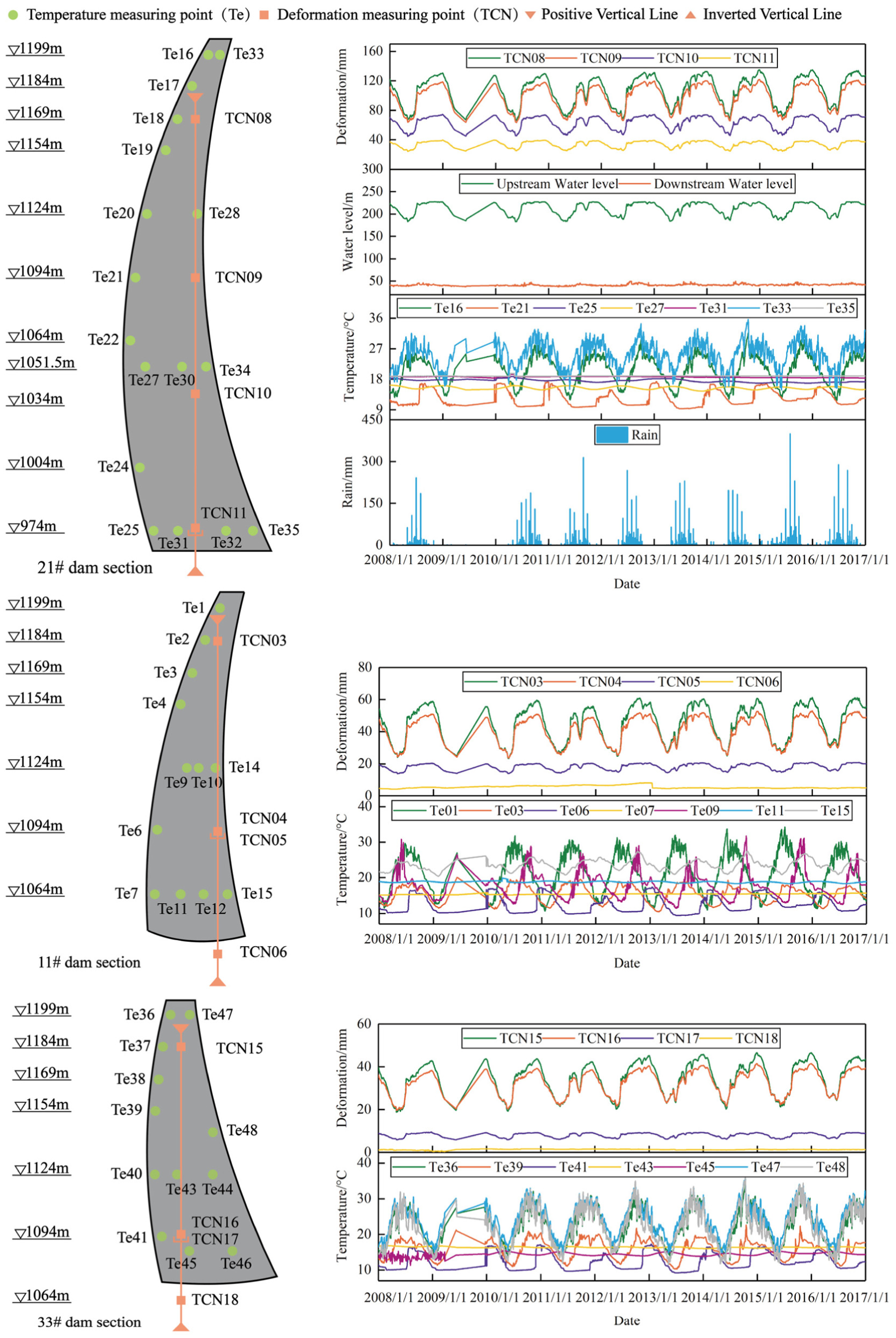
Monitoring layout and time histories of dam deformation and environmental variables.
Model parameter settings and optimizer comparison
Hyperparameter search space
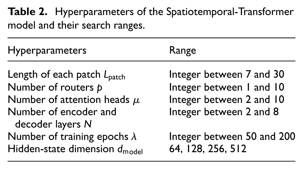
Table 2 summarizes the hyperparameters of the Spatiotemporal-Transformer model and their search ranges. These hyperparameters control the temporal resolution, spatial information exchange, model capacity, and training process of the proposed model. Specifically, the patch length
Hyperparameters of the Spatiotemporal-Transformer model and their search ranges.
Comparison of hyperparameter optimizers
To provide an independent assessment of the contribution of SAO to hyperparameter optimization, SAO was compared with three widely used optimization methods, namely, Bayesian optimization (BO), PSO, and GA. For a fair comparison, all optimizers used the same hyperparameter search space, training/validation/test split, fitness function, and maximum number of function evaluations.
Figure 8 shows the convergence curves of different optimizers during hyperparameter search. The curves represent the best-so-far validation
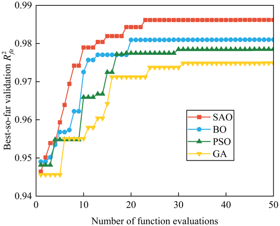
Convergence curves of different hyperparameter optimizers during hyperparameter search.
Based on the above optimizer comparison, SAO was selected to determine the final hyperparameter configuration of the Spatiotemporal-Transformer model. The hyperparameter set
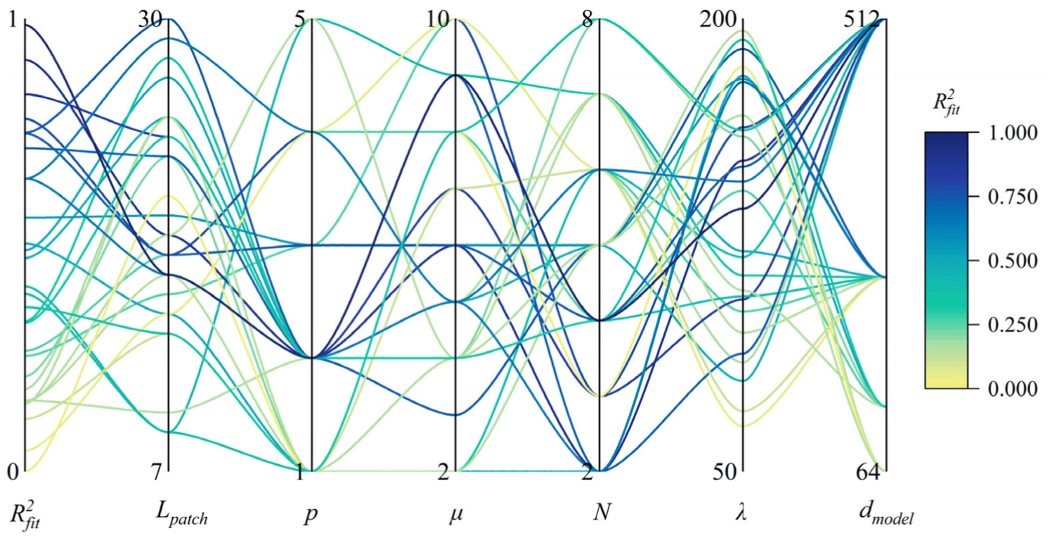
Correspondence between hyperparameter sets and validation
Visual analysis of model predictions
Evaluation metrics
Before presenting the prediction results, four evaluation metrics were used to quantify the prediction performance at each deformation monitoring point, including the coefficient of determination (R2), mean absolute error (MAE), mean squared error (MSE), and root-mean-squared error (RMSE). It should be noted that
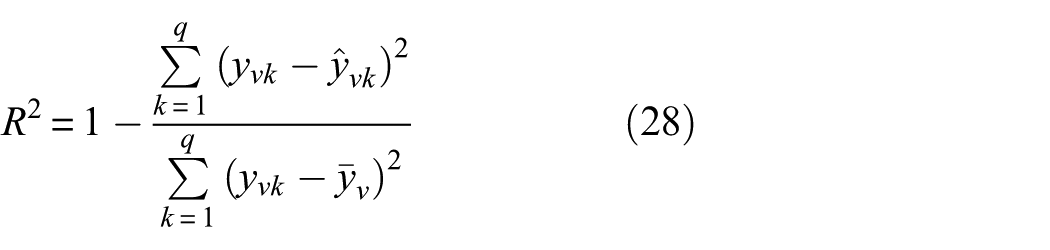



where
Ablation experiment
A systematic ablation study was conducted to quantify the individual contribution of each key component in the proposed SAO-STformer framework. Table 3 summarizes the model variants used in the ablation experiments. The full proposed model contains five key components: multivariate patch embedding, temporal attention, routing-based spatial attention, scale fusion, and SAO-based hyperparameter optimization. The variants denoted as “w/o multivariate patch embedding,”“w/o spatial attention,”“w/o scale fusion,” and “w/o SAO” were designed by removing the corresponding module while keeping the remaining components unchanged. In addition, PSO+Spatiotemporal-Transformer, Transformer, PSO+Transformer, and SAO + Transformer are included to further distinguish the effects of the proposed Spatiotemporal-Transformer architecture and the optimization strategy.
Definitions of ablation configurations.
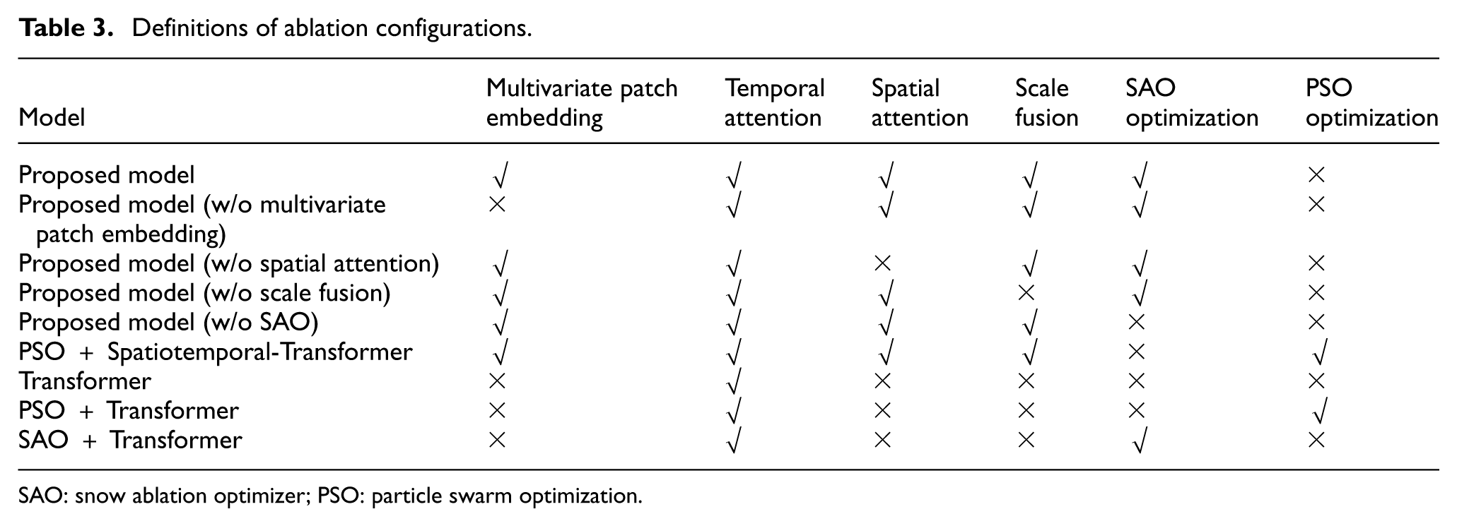
SAO: snow ablation optimizer; PSO: particle swarm optimization.
Figure 10 and Table 4 summarize the predictive performance of the proposed model and eight ablation models across multiple monitoring points. The evaluation considers both model accuracy, represented by R2, and error metrics, including MAE, MSE, and RMSE. The experimental results indicate that the proposed model achieves the best overall performance across all monitoring points. Regarding model accuracy, its R2 value consistently remains within the high range of 0.978 to 0.986, with absolute improvements ranging from 0.006 to 0.071 over the ablation models. Notably, the performance at the TCN03 monitoring point is particularly remarkable, exhibiting improvements of 0.034 and 0.071 over the proposed model (w/o SAO) and Transformer, respectively. This result indicates that the proposed framework can better capture complex nonlinear deformation features. Regarding error control, the proposed model also demonstrates clear advantages. At the TCN05 monitoring point, the MAE is 0.201, reflecting a 21.2% reduction compared with the second-best model, that is, the proposed model (w/o scale fusion) with an MAE of 0.255. The RMSE is 0.237, representing a 22.3% reduction compared with the proposed model (w/o scale fusion) and a 53.6% reduction compared with PSO + Transformer. At the more challenging TCN08 monitoring point, the MSE of the proposed model is only 29.2% that of the Transformer, providing strong evidence of the model’s advantage in suppressing large prediction errors.
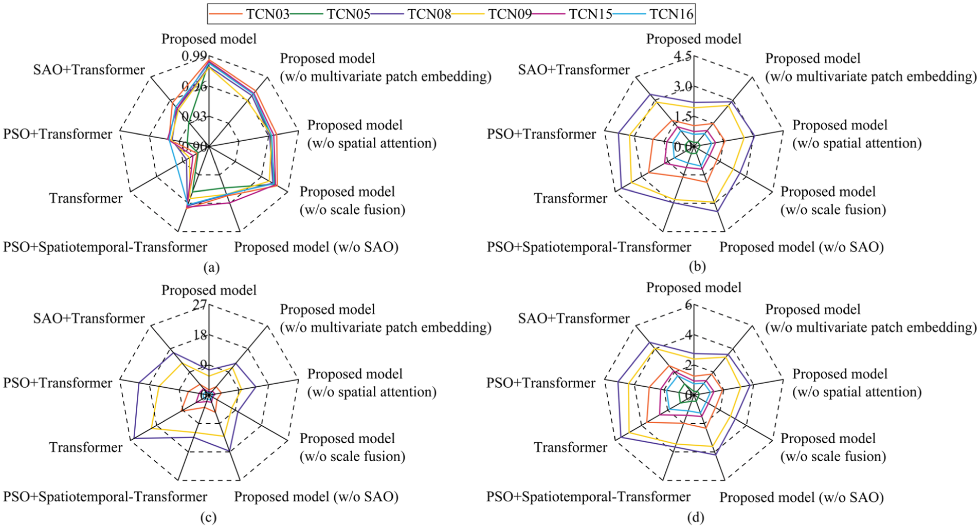
Comparison of evaluation indices in the ablation experiments: (a) R2, (b) MAE, (c) MSE, and (d) RMSE. MAE: mean absolute error; MSE: mean squared error; RMSE; root-mean-squared error.
Summary of evaluation indicators for the ablation experiments.
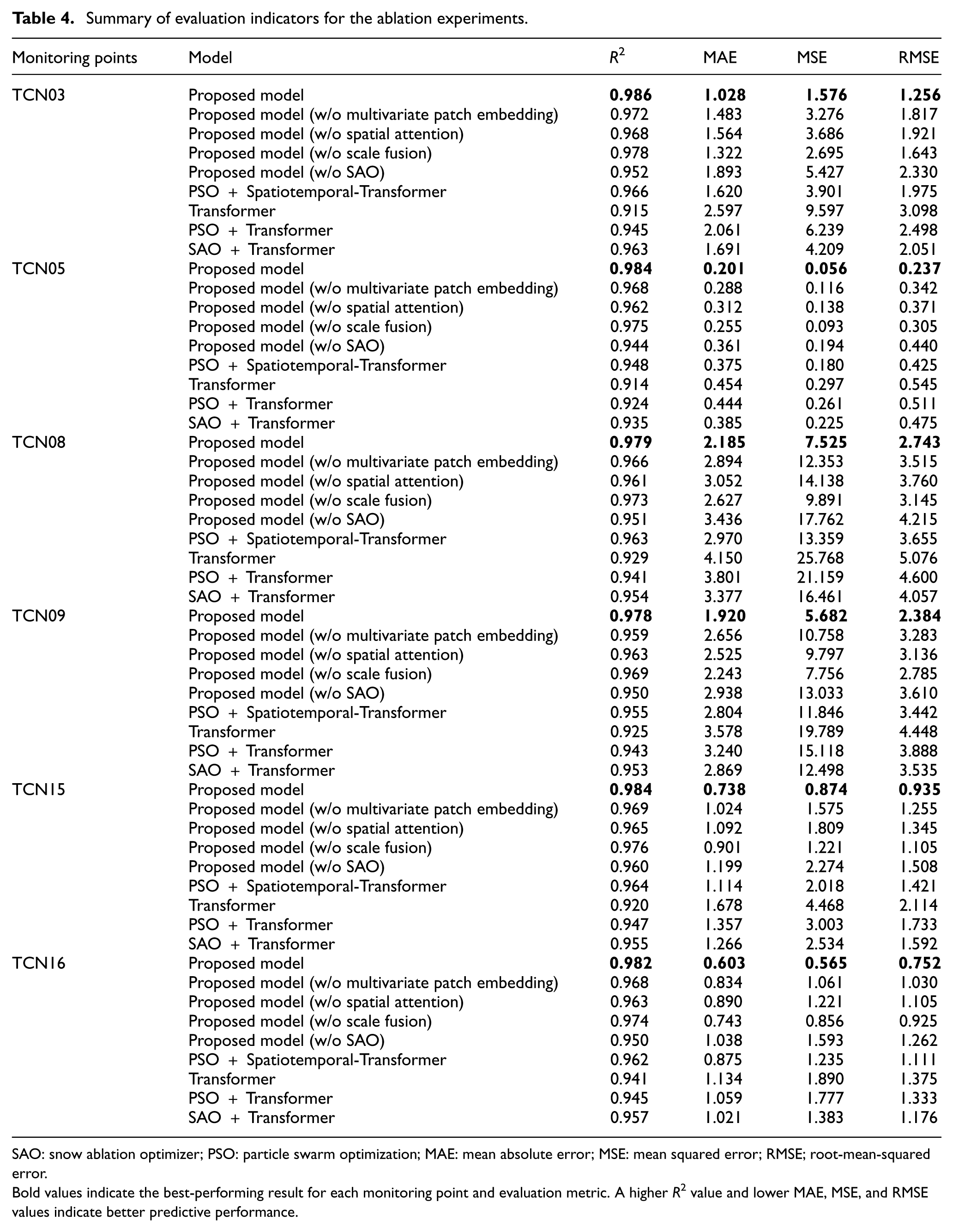
SAO: snow ablation optimizer; PSO: particle swarm optimization; MAE: mean absolute error; MSE: mean squared error; RMSE; root-mean-squared error.
Bold values indicate the best-performing result for each monitoring point and evaluation metric. A higher R2 value and lower MAE, MSE, and RMSE values indicate better predictive performance.
The component-level ablation results further reveal the contribution of each module. Removing multivariate patch embedding, spatial attention, scale fusion, or SAO leads to different degrees of performance degradation, confirming that these components jointly contribute to spatiotemporal feature extraction and multiscale dependency modeling. Among the three structural components, removing spatial attention generally causes a more pronounced performance decline at most monitoring points, indicating that the modeling of intervariable spatial dependencies is important for multipoint dam deformation prediction. The removal of scale fusion results in a relatively smaller but still consistent performance degradation, suggesting that multiscale representation further enhances the model’s ability to capture both short-term fluctuations and long-term deformation trends.
In addition, the comparison among the proposed model, proposed model (w/o SAO), PSO + Spatiotemporal-Transformer, Transformer, PSO + Transformer, and SAO + Transformer demonstrates the importance of hyperparameter optimization. The proposed model (w/o SAO) shows a clear performance decrease compared with the full model, indicating that an appropriate hyperparameter configuration is essential for fully exploiting the representation capacity of the Spatiotemporal-Transformer architecture. Moreover, the proposed model consistently outperforms PSO + Spatiotemporal-Transformer, confirming that SAO provides a more effective hyperparameter search strategy than PSO under the same model architecture. These results further demonstrate that the performance gain of SAO-STformer is derived from both the proposed spatiotemporal architecture and the SAO-based optimization strategy.
Performance comparison with the baseline models
To rigorously validate the model’s superior performance, comprehensive comparative experiments are conducted against six benchmark methods: Informer, Reformer, RF, support vector regression (SVR), MLP, and CatBoost.
The left section of Figure 11 illustrates the deformation prediction process lines at various monitoring points from June 2015 to January 2017. As shown in the figure, the prediction curve of the proposed model closely aligns with the trend of the monitoring data, demonstrating its robust prediction capability at various monitoring points. In comparison to the benchmark models, the proposed model better captures the deformation dynamics over time, achieving a higher overall fit. This suggests that the proposed model performs more effectively in capturing deformation trends and periodic fluctuations. The scatter plot on the right-hand side of Figure 11 further demonstrates the superior performance of the proposed model. As shown in the figure, a strong linear correlation exists between the model’s predicted values and the monitored values, with data points closely clustered around the reference line y = x, suggesting negligible prediction errors. Furthermore, the maximum residual serves as a crucial indicator for model evaluation. In practical engineering applications, large residuals may suggest that the model struggles to predict extreme environmental changes or irregular fluctuations. The maximum residual of the proposed model shows limited variation across different measurement points, with a minimum value of 0.600 mm occurring at the TCN05 monitoring point, indicating that the model demonstrates strong predictive capability.
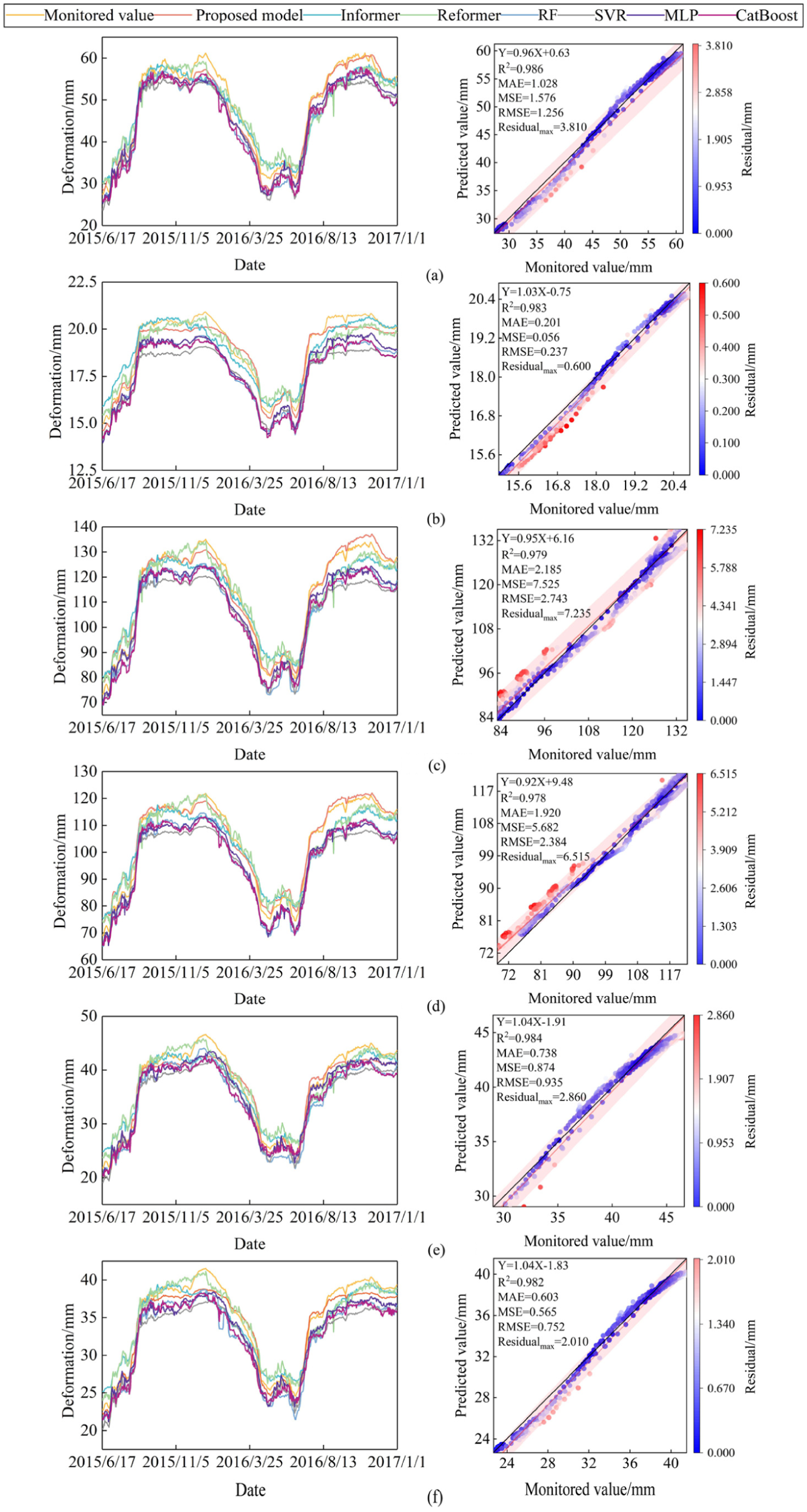
Prediction process lines and maximum residuals: (a) TCN03, (b) TCN05, (c) TCN08, (d) TCN09, (e) TCN15, and (f) TCN16.
Figure 12 and Table 5 illustrate the radial bar charts of evaluation metrics for various models. The radial bar chart is a polar-coordinate visualization, with the origin at the center and the circumference divided into angular segments. Compared to Cartesian coordinates, it offers an improved visualization of the differences and trends across various models for different evaluation metrics. As depicted in the figure, the proposed model demonstrates substantial advantages across all monitoring points. Specifically, at the TCN03, TCN05, TCN15, and TCN16 monitoring points, the RMSE, MAE, and MSE values for the proposed model are notably lower than those of other benchmark models, with R2 values approaching or exceeding 0.98, indicating high precision and strong model fit. In contrast, the prediction accuracy of SVR and RF is generally lower, particularly at the TCN05 monitoring point, where SVR’s R2 is only 0.417, significantly lower than that of the proposed model. At the TCN08 and TCN09 monitoring points, the proposed model exhibits relatively higher errors, with RMSE values of 2.743 and 2.384, respectively. However, it still significantly outperforms other benchmark models, with RMSE values exceeding 4.0 for Informer and Reformer, and surpassing 6.0 for SVR, RF, MLP, and CatBoost. In conclusion, the proposed model achieves superior performance compared to both conventional machine learning methods and Transformer variants.
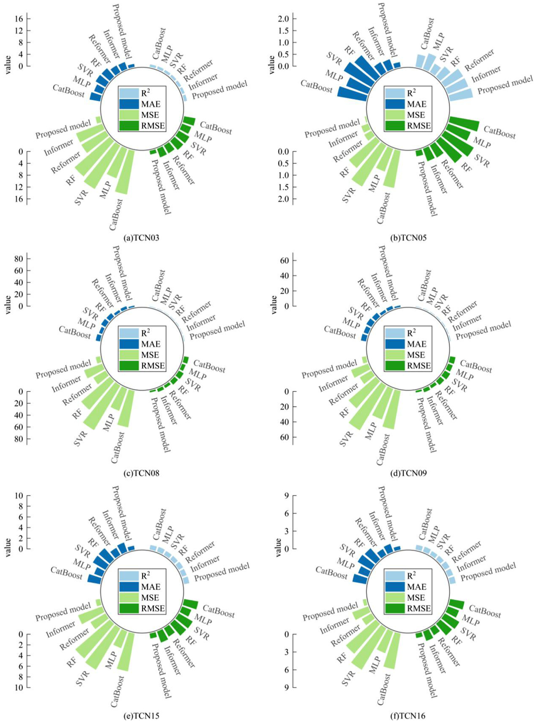
Radial bar charts of evaluation metrics for various models: (a) TCN03, (b) TCN05, (c) TCN08, (d) TCN09, (e) TCN15, and (f) TCN16.
Summary of evaluation indices for comparison models.
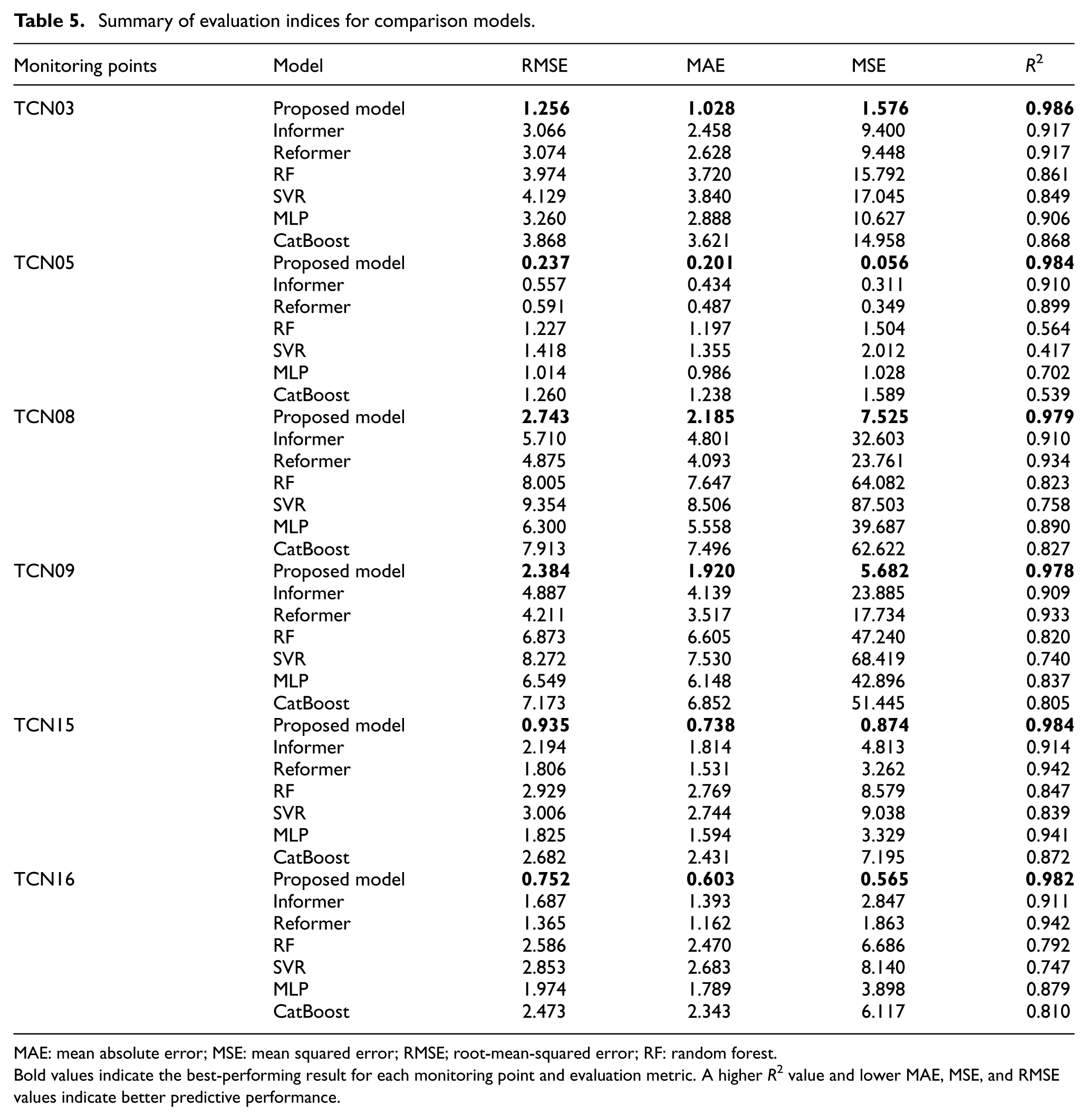
MAE: mean absolute error; MSE: mean squared error; RMSE; root-mean-squared error; RF: random forest.
Bold values indicate the best-performing result for each monitoring point and evaluation metric. A higher R2 value and lower MAE, MSE, and RMSE values indicate better predictive performance.
Figure 13 presents the residual raincloud plots for various models. Each subplot comprises three components: a kernel density plot, a box plot, and a bee swarm plot. The upper layer of the raincloud plot represents the kernel density plot, which forms a smooth probability density curve by placing Gaussian kernel functions around each data point and superimposing them, visually illustrating the density distribution of the data. The middle box plot reveals the median and quartiles of the data, aiding in understanding data dispersion and abnormal fluctuations. The lower bee swarm plot shows the distribution of residual values through dispersed, ordered scatter points, avoiding overlap and offering a clearer view of local density. From the figure, it is evident that the residuals of the proposed model are evenly distributed and close to zero, demonstrating strong fitting performance. This indicates that the proposed model effectively captures the spatiotemporal variation trends of deformation data, with predictions closely matching the monitored values and exhibiting minimal deviation. In contrast, the residuals of benchmark models exhibit significant irregular fluctuations, particularly at the TCN03, TCN08, and TCN16 monitoring points, where the residual distributions are more dispersed and exhibit greater fluctuation, indicating large fitting errors. These models fail to capture the overall trend of the data effectively, leading to a substantial gap between predicted and monitored values.
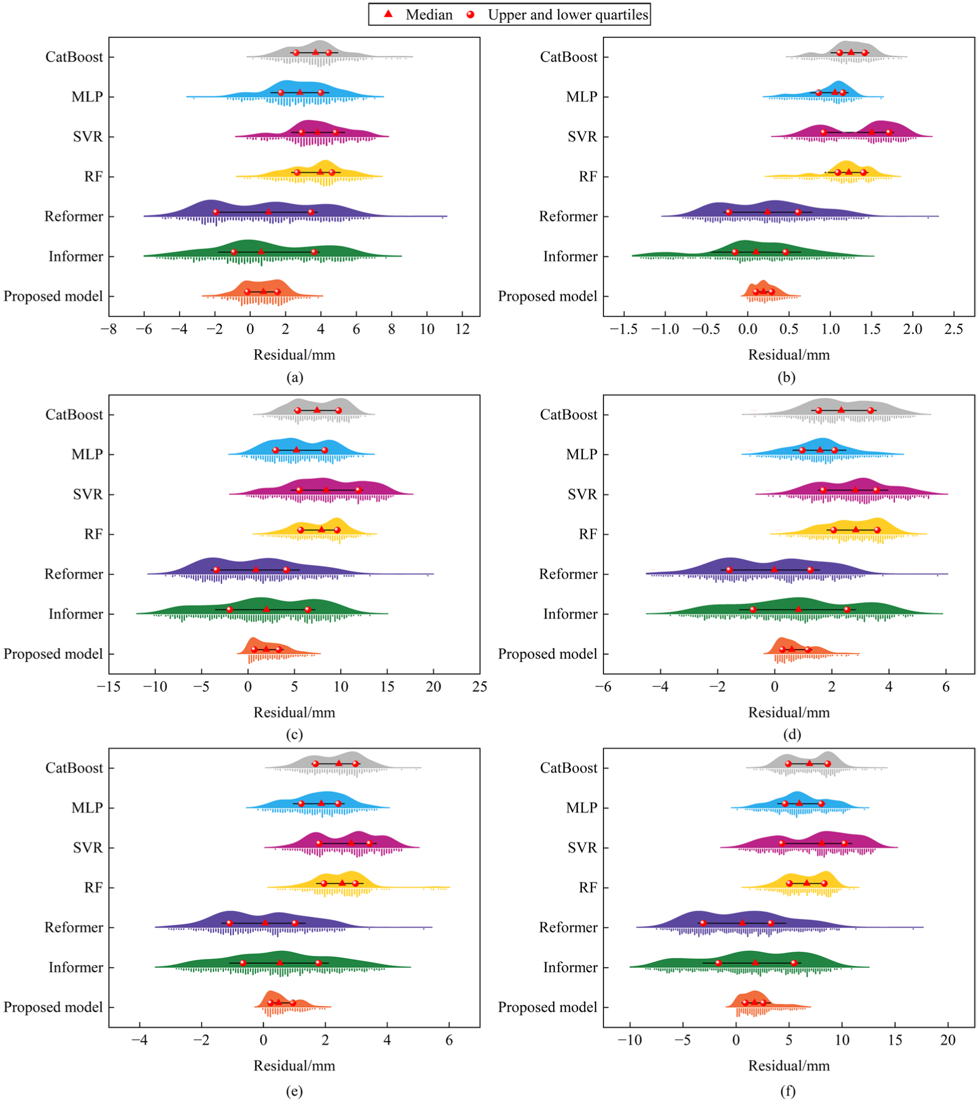
Residual raincloud plots: (a) TCN03, (b) TCN05, (c) TCN08, (d) TCN09, (e) TCN15, and (f) TCN16.
Cross-validation for generalization analysis
To further evaluate the generalization ability of the proposed model, a rolling-origin time-series cross-validation experiment was conducted. Unlike random k-fold cross-validation, the chronological order of the monitoring data was strictly preserved to avoid information leakage. As shown in Table 6, four folds were constructed using an expanding training window. In each fold, the model was trained using historical monitoring data, tuned on the subsequent validation year, and evaluated on the following test year.
Settings of rolling-origin time-series cross-validation.

Table 7 presents the cross-validation results of the proposed model and the benchmark models. The reported R2 value of each fold represents the average prediction accuracy over the six deformation monitoring points. The proposed model achieves the highest R2 values in all four folds, with R2 values of 0.971, 0.976, 0.974, and 0.981, respectively. Its mean R2 reaches 0.976, which is higher than that of the benchmark models. In addition, the proposed model obtains a low standard deviation of 0.003 across the four folds, indicating that its prediction performance remains stable under different testing periods. The cross-validation results further demonstrate that the proposed model is not only effective under a fixed training–test split but also maintains robust predictive performance across different operation periods.
Results of the time-series cross-validation.
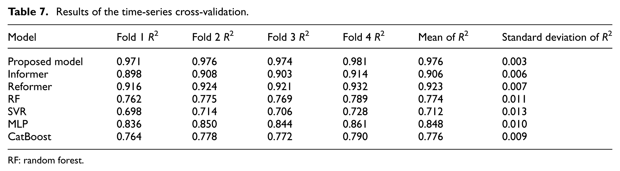
RF: random forest.
Visual analysis of the spatiotemporal attention mechanism
In the previous subsections, the predictive performance of multiple models was evaluated on identical datasets, and differences in their outcomes were examined. The results indicate that, among the models tested, attention-based architectures achieved the highest performance. To further investigate the proposed SAO-STformer model, the environmental variables and spatiotemporal attention weights are visualized in this section, followed by an analysis of their trends and overall distributions.
Figure 14 illustrates the distribution of temporal attention weights for deformation measurement points at various locations on the dam. The x-axis represents the time steps within the input window, while the values from 1 to 49 on the y-axis correspond to the 49 environmental variables defined in Equation (27). As shown in the figure, the proposed model dynamically adjusts the attention weights for different environmental variables at each time step, effectively capturing the relative importance of each variable in deformation prediction.
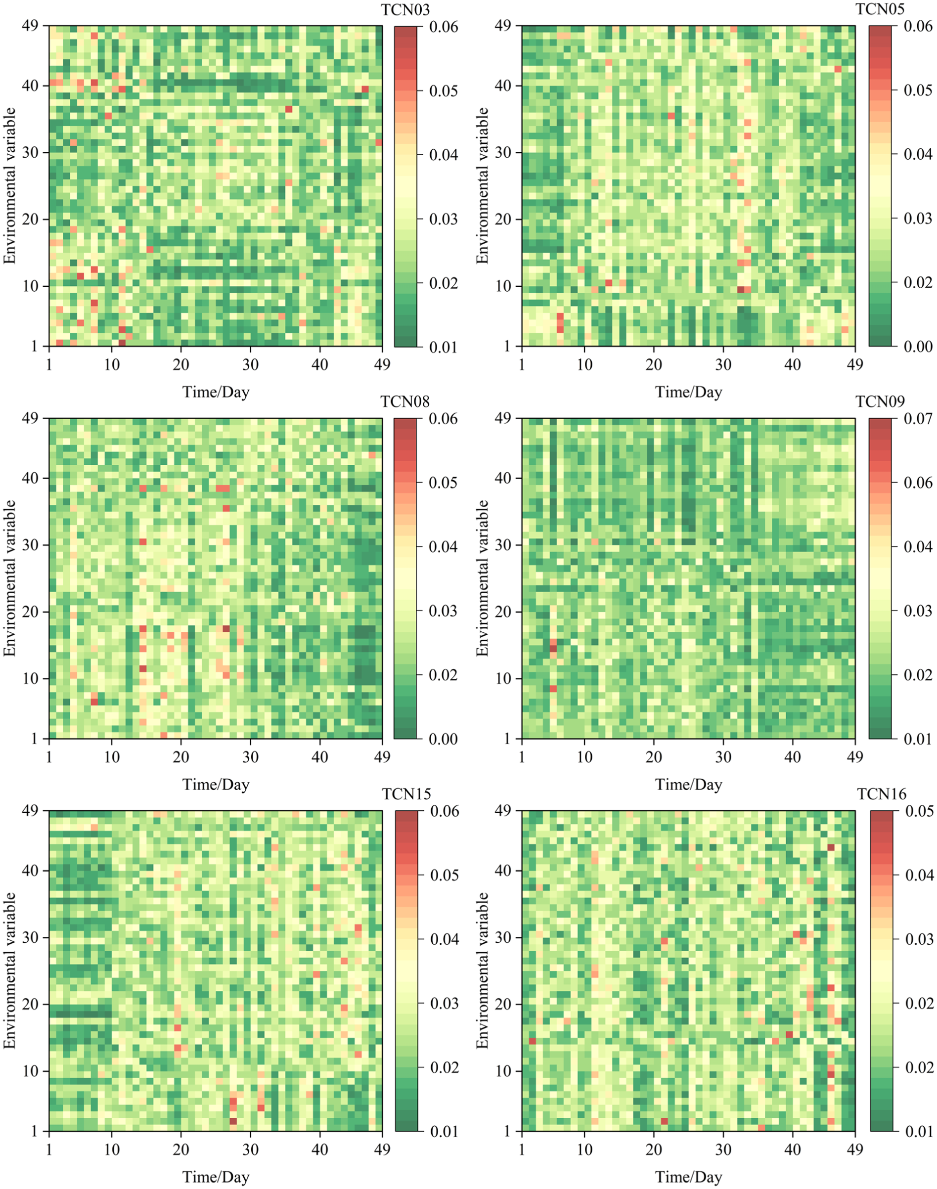
Visualization of temporal attention weights.
To further provide a quantitative interpretation, the 49 input variables were grouped according to their physical correspondence with the three HTT-related deformation components. Specifically,
Table 8 summarizes the normalized group-averaged temporal attention weights for the water-pressure, temperature, and aging components. The results show that the temperature component generally receives relatively high attention weights, such as 0.388, 0.371, 0.383, 0.370, and 0.349 at TCN03, TCN05, TCN08, TCN15, and TCN16, respectively. This is physically consistent with dam deformation mechanisms, because temperature variations can induce thermal expansion and contraction of concrete. More importantly, the temperature field usually exhibits a pronounced seasonal pattern that is highly consistent with the periodic fluctuation of dam deformation. Therefore, temperature-related variables provide important information for identifying the long-term cyclic deformation trend and delayed thermal response of the dam body. During periods when reservoir water level changes are relatively gradual but seasonal temperature fluctuations are significant, the temperature component may, therefore, receive higher attention than the water-pressure component. These results suggest that the temporal attention mechanism substantially enhances the model’s predictive accuracy by dynamically identifying key environmental variables during periods of significant deformation changes.
Quantitative interpretation of normalized temporal attention weights by HTT-related components.
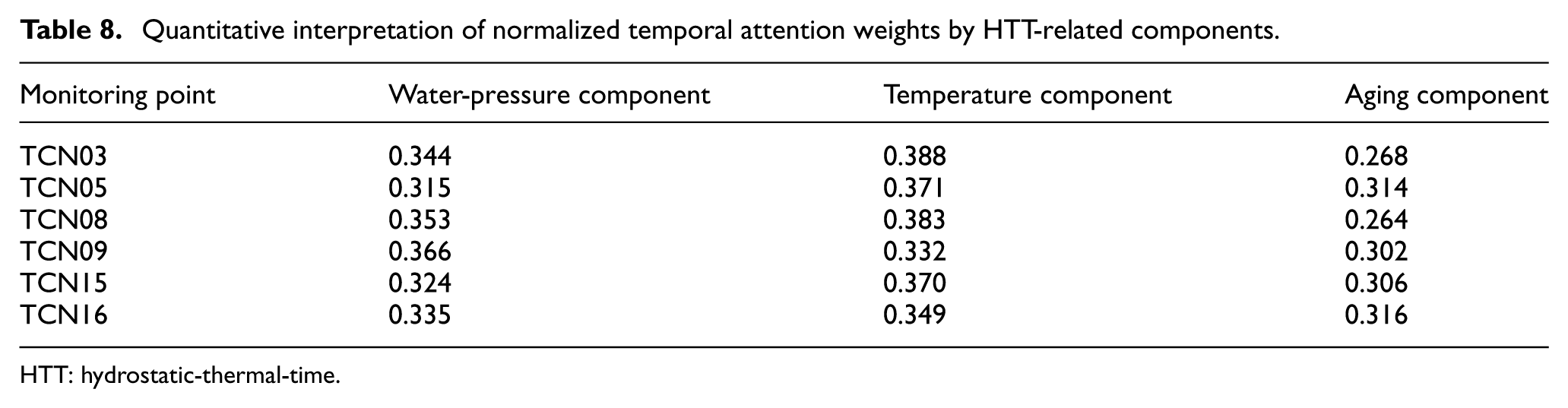
HTT: hydrostatic-thermal-time.
Figure 15 presents the visualization of spatial attention weights for deformation measurement points at various locations on the dam. The x and y coordinates, ranging from 1 to 49, correspond to the 49 environmental variables defined in Equation (27). Unlike temporal attention, which describes the importance of each variable at different time steps, spatial attention reflects the interaction strength between different environmental variables. Therefore, higher values in Figure 15 indicate that the model assigns stronger attention to the coupling relationship between two variables when predicting deformation at a given monitoring point.
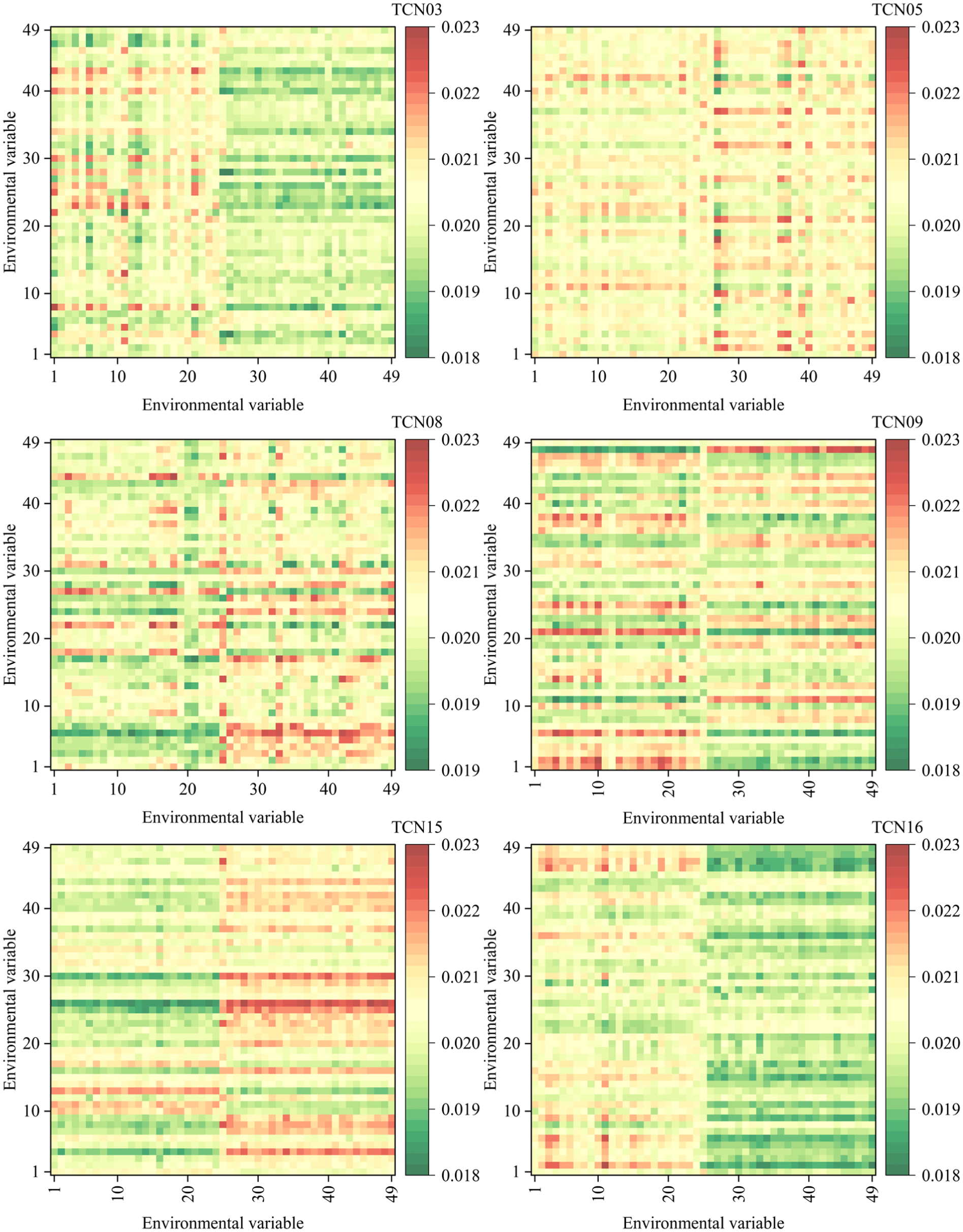
Visualization of spatial attention weights.
As illustrated in Figure 15, the spatial attention maps show clear block-like patterns rather than uniformly distributed weights, indicating that the model captures structured interactions among the water-pressure, temperature, and aging components. In particular, the monitoring points located near the riverbed section, such as TCN08 and TCN09, exhibit relatively stronger spatial attention associated with water-pressure–temperature interactions. This pattern is physically reasonable because the riverbed section is subjected to stronger hydrostatic pressure and more pronounced constraint effects from the dam foundation and surrounding concrete, making its deformation more sensitive to the coupled effects of reservoir water level and temperature. For the bank-section monitoring points, such as TCN03, TCN05, TCN15, and TCN16, the spatial attention distribution is relatively more dispersed, suggesting that their deformation responses are jointly affected by temperature variation, local structural constraints, and long-term trend components rather than being dominated by water pressure alone.
The analysis of the spatiotemporal attention weights not only identifies the key environmental factors influencing dam deformation but also uncovers the dynamic coupling mechanism among these variables in greater detail. Nevertheless, attention weights should be interpreted as model-based indicators of relative importance and intervariable association, rather than as direct causal effects or exact mechanical contribution ratios. Overall, the temporal attention results are consistent with the HTT-related deformation components and seasonal effects, while the spatial attention results further reflect the structural-zone differences and cross-variable coupling characteristics of dam deformation. These findings provide essential theoretical foundations and practical support for decision-making in dam safety monitoring and hazard mitigation.
Conclusions and future work
This study introduces SAO-STformer, an innovative architecture for dam deformation prediction. Its superior predictive performance was demonstrated through systematic ablation studies, comparative evaluations, and a cross-validation experiment, which further verified the model’s generalization ability across different operation periods. The model integrates the Spatiotemporal-Transformer and the SAO algorithm to improve the extraction of spatiotemporal features. The Spatiotemporal-Transformer systematically optimizes three key Transformer components: the multivariate patch embedding, the spatiotemporal attention mechanism, and the progressive encoder–decoder structure. These enhancements enable the model to capture spatiotemporal features and long-term dependencies simultaneously, thereby achieving superior prediction accuracy. Additionally, the SAO algorithm employs a dual-population mechanism, which facilitates the optimization of the Spatiotemporal-Transformer’s hyperparameters.
Experimental results indicate that the proposed model significantly outperforms conventional machine learning methods in prediction accuracy across all monitoring points and comprehensively surpasses existing Transformer variants in various evaluation metrics. The R2 value of the proposed model consistently remains within the high range of 0.978–0.986. The residuals are close to zero and uniformly distributed. The cross-validation results further confirm its stable generalization ability, with the highest R2 values in all four folds, a mean R2 of 0.976, and a low standard deviation of 0.003. In addition, a physical interpretation based on the spatiotemporal attention mechanism is presented. Analysis of the attention weights reveals that temperature variables exhibit high attention values, indicating the substantial impact of temperature variations on dam displacement. A pronounced spatial attention weight between the reservoir water level and temperature variables highlights their strong spatial coupling effect on dam deformation. This study presents a novel theoretical foundation and intelligent decision-making tools for enhancing the safety monitoring and reinforcement of high arch dams.
Although the proposed SAO-STformer shows promising performance, several limitations should be further addressed. First, although the risk of overfitting was mitigated in this study through hyperparameter optimization, ablation analysis, and independent testing, deep learning models may still be sensitive to limited monitoring samples and noise contamination. Future work will further evaluate the robustness of the proposed model under noisy and incomplete monitoring data. Second, although SAO improves prediction accuracy, its dual-population search mechanism requires repeated fitness evaluation and individual ranking, increasing computational cost. Future work should explore lightweight SAO variants for large-scale monitoring systems. Third, the model performance may be sensitive to key hyperparameters, especially the patch length
Footnotes

Funding
The authors disclosed receipt of the following financial support for the research, authorship, and/or publication of this article: This research was supported by the National Natural Science Foundation of China (nos. 52579119, 52379122, and 52508277), the National Key Research and Development Program (no. 2024YFC3210700), the Jiangsu Provincial Natural Science Foundation Youth Project (no. BK20250697), and the Xizang Autonomous Region Science and Technology Funding (no. XZ202501ZY0009).
Declaration of conflicting interests
The authors declared no potential conflicts of interest with respect to the research, authorship, and/or publication of this article.