A modal decomposition method of adaptively constructing empirical wavelet filter banks and its application in rotating machinery fault diagnosis

Abstract

The empirical wavelet transform (EWT) method has shown a broad application prospect in the fault diagnosis of rotating machinery. However, it has the problem that the number of modes needs to be preset, and the spectrum segmentation is unreasonable under strong noise. To this end, this paper proposes a modal decomposition method of adaptively constructing empirical wavelet filter banks, which is named adaptive empirical wavelet filter banks (AEWFMD). Firstly, the spectrum trend line is constructed by calculating the energy mean of the Stockwell Transform spectrum along the frequency slice. Secondly, the proposed optimized fault feature energy ratio (OFCER) is used as the objective function, and the smoothing window of the order-statistic filtering is optimized to obtain the optimal spectral line. Then, taking the position of the minimum point of the optimal spectral line as the boundary, it divides the spectrum scientifically and adaptively constructs the empirical wavelet filter bank to reconstruct the modal components. Finally, the optimal modal component is selected based on the OFCER index, and its normalized envelope spectrum analysis is performed. Simulation and experimental results show that AEWFMD can adaptively determine the segmentation boundary and the number of modes. Compared with EWT, empirical Fourier decomposition (EFD), and Feature Mode decomposition (FMD) methods, AEWFMD performs better in single and compound fault feature extraction, which provides a new path for bearing fault diagnosis in engineering practice.

Keywords

rolling bearings fault diagnosis empirical wavelet filter Stockwell Transform spectrum spectrum trend line

Introduction

Rolling bearings are core components of rotating machinery and are widely utilized across modern industrial sectors.^1–4 However, due to prolonged operation under harsh environments, varying operating conditions, and alternating loads, rolling bearings inevitably suffer from various types of failures.^5,6 Such abrupt faults not only lead to equipment downtime and damage but may also result in severe economic losses or even catastrophic consequences.⁷ Consequently, investigating high-precision fault diagnosis methods for rolling bearings has become an urgent priority. In engineering practice, early local damage in bearings typically manifests as a series of weak impulsive features.⁸ Nevertheless, these characteristic signals are often masked by intense background noise and complex interference, making fault extraction extremely challenging. In summary, conducting in-depth research into rolling bearing fault diagnosis is of significant theoretical importance and engineering value for ensuring the safe operation of equipment.⁹

In recent years, intelligent fault diagnosis technology has flourished. Within this field, deep learning has demonstrated significant advantages in industrial equipment monitoring due to the superior feature extraction capabilities of convolutional neural networks (CNNs).^10,11 At the signal processing level, time-frequency analysis methods based on the Stockwell Transform (ST) have attracted considerable attention due to their unique merits. By introducing a frequency-dependent Gaussian window, ST effectively overcomes the limitations of the fixed window length in the short-time Fourier transform and the lack of phase information in the wavelet transform (WT), achieving a multi-resolution time-frequency representation.^12–14 ST can transform a one-dimensional vibration signal into a two-dimensional energy time-frequency spectrum, where the energy distribution precisely characterizes the evolutionary features of different frequency components over time. Exploiting this property, Ying et al.¹⁵ proposed an ST spectral amplitude modulation method, experimentally confirming the comprehensiveness and accuracy of ST spectral energy values in characterizing fault information. Building on this, Liu et al.¹⁶ further introduced a second-order transient extraction S-transform, significantly enhancing the sensitivity of health status monitoring for critical components. Interdisciplinary research has also validated the robustness of ST: Xie et al.¹⁷ and Xiao et al.¹⁸ achieved high-precision identification in EEG signal classification and power grid fault diagnosis, respectively, by combining CNNs with attention-enhanced ST frameworks and multi-resolution ST spectra. Furthermore, Shi et al.¹⁹ utilized ST spectra as inputs for a multi-task deep learning network in near-infrared spectroscopy, successfully predicting complex components. Collectively, these studies indicate that the ST spectrum can highly restore the time-frequency distribution characteristics of signals through energy mapping, reflecting the fault information distribution level along each frequency over time in the form of energy values.

Due to the high sensitivity and accessibility of vibration signals regarding mechanical faults, vibration analysis has become a core technique in rotating machinery fault diagnosis.^20,21 However, in practical industrial scenarios, rolling bearings often operate under complex conditions, causing weak fault features to be easily submerged by strong background noise, which increases the difficulty of information extraction.²² To decouple fault features from non-stationary interference, signal decomposition techniques have advanced significantly. Among them, empirical mode decomposition (EMD) is a representative method capable of adaptively decomposing a signal into a series of intrinsic mode functions (IMFs) based on the signal’s local characteristics.²³ Although EMD exhibits excellent time-frequency aggregation when processing non-stationary signals, the envelope interpolation method used in its theoretical framework inevitably introduces end effects and mode mixing. To address these deficiencies, Wu et al.²⁴ proposed ensemble EMD (EEMD), which suppresses mode mixing by injecting white noise into the original signal to assist the decomposition. While EEMD improves the mixing phenomenon, it suffers from residual noise in the modal components because the noise cannot be completely canceled. Consequently, Yeh et al.²⁵ proposed Complementary EEMD (CEEMD), using a strategy of adding pairs of noise with opposite polarities to reduce residual noise. Subsequently, Torres et al.²⁶ developed CEEMD with adaptive noise, which achieves quasi-lossless signal reconstruction by adding specific noise to the residues of each decomposition stage and taking the average. Additionally, regarding sine-assisted decomposition, Ying et al.²⁷ proposed Permutation Entropy-based Uniform Phase EMD, utilizing uniform phase sinusoidal signals to resolve mixing and applying the permutation entropy criterion to precisely screen characteristic components. Despite the progress made by these improved algorithms, there remains room for enhancement in decomposition accuracy and computational stability.

To overcome the inherent mode mixing and end effects of EMD, Dragomiretskiy and Zosso²⁸ proposed variational mode decomposition (VMD). By solving a constrained variational model, this method adaptively decouples complex signals into a series of quasi-orthogonal band-limited IMFs with specific center frequencies. Although VMD performs excellently in suppressing mixing, its effectiveness is highly dependent on the preset number of decomposition levels, and the process of screening specific fault components in multi-modal scenarios remains cumbersome. To address this limitation, Nazari et al.²⁹ proposed variational mode extraction (VME), which partitions a signal directly into a target mode and a residual component based on a minimum energy overlap criterion. Compared to VMD, VME offers advantages in computational overhead and targeted feature extraction, though it remains sensitive to the initial center frequency settings. Furthermore, to capture non-linear features more comprehensively while maintaining structural stability, Pan et al.³⁰ introduced symplectic geometry mode decomposition (SGMD), demonstrating superior separation capabilities in compound fault diagnosis. To tackle the bottleneck of extracting periodic impulses under strong noise, Pan et al.³¹ proposed a Periodic Segmental Symplectic Geometry Transform, adaptively optimizing parameters via a neighborhood peak method to enhance the extraction accuracy of bearing fault pulses. Hybrid approaches have further bolstered SGMD: Cheng et al.³² combined symplectic similarity transforms with Ramanujan subspace theory to achieve precise compound fault separation using hierarchical clustering, while Guo et al.³³ introduced cyclic kurtosis entropy to construct an adaptive SGMD framework for weak feature extraction. To further reinforce de-noising, Li et al.³⁴ combined enhanced maximum entropy deconvolution with adaptive SGMD, achieving robust diagnosis of complex rolling bearing fault states.

Diverging from the aforementioned philosophies, Gilles³⁵ combined spectral segmentation with an empirical wavelet filter bank to propose the empirical WT (EWT). This method is supported by a rigorous mathematical framework and largely overcomes mode mixing. However, the performance of standard EWT is highly dependent on the preset number of modes and is susceptible to spectral noise, which often leads to overly dense boundary segmentation. To address these limitations, researchers have explored various improvements. Wang et al.³⁶ introduced a sparsity-guided mechanism for boundary partitioning, though parameter optimization remains challenging. To enhance adaptivity, Pan et al.³⁷ proposed modified EWT, identifying local minima through the inner product of the Fourier spectrum and Gaussian functions, albeit at an increased computational cost. To suppress spectral noise, Luo et al.³⁸ used the Burg algorithm to extract an auto-regressive power spectrum to replace the original spectrum, improving partitioning accuracy. Subsequently, Hu et al.³⁹ proposed Enhanced EWT by applying order filtering to the spectral upper envelope, though an optimal criterion for envelope selection was not established. Additionally, Xu et al.⁴⁰ utilized the spectral trend to guide boundary selection, constructing a trend line by iteratively calculating the mean of upper and lower envelope functions. Nevertheless, achieving reasonable and robust spectral segmentation remains the core challenge affecting decomposition performance.

In summary, despite the significant success of EWT and its variants in feature extraction, several critical challenges remain to be addressed: Issues in Spectral Segmentation: (1) Traditional EWT methods rely heavily on the morphological characteristics of the spectrum for interval partitioning. Under noisy conditions, the spectrum is prone to severe distortion, leading to “over-segmentation” and subsequent inaccuracies in the construction of the empirical wavelet filter bank. (2) Lack of Parameter Self-Adaptability: Current methods lack an efficient, data-driven strategy to dynamically adjust the number of modes or filter parameters, which restricts the algorithm’s adaptive capacity in signal processing. (3) Incomplete Evaluation Criteria for Sensitive Components: Among the decomposed modal components, the absence of evaluation indices sensitive to fault features makes the automated selection of the optimal diagnostic component somewhat arbitrary.

Accordingly, this paper proposes a modal decomposition method for constructing adaptive empirical wavelet filter banks (AEWFMD). First, leveraging the superior time-frequency aggregation of the ST, a spectral trend line representing the macroscopic energy distribution is constructed by calculating the mean energy along the frequency axis. Second, an optimized fault characteristic energy ratio (OFCER) is proposed as an objective function to guide the adaptive selection of the smoothing window for an order-statistic filtering (OSF), thereby obtaining an optimal spectral line that balances local features with global smoothness. Subsequently, the local minima of the optimal spectral line are used as segmentation boundaries to adaptively construct the empirical wavelet filter bank and reconstruct modal components. Finally, the best mode is automatically identified from the reconstructed components based on the OFCER indicator, followed by normalized envelope spectrum analysis to extract bearing fault characteristics.

The novelties of this paper are summarized as follows:

Construction of a robust spectral trend line based on ST energy distribution. To address the sensitivity of EWT to noisy transients, the multi-resolution property of ST is leveraged to map high-dimensional time-frequency distributions into macroscopic trend lines via mean energy calculation. This mechanism suppresses impulsive noise through energy evolution, establishing a robust physical foundation for subsequent adaptive spectral boundary partitioning.

Parameter adaptive optimization driven by the OFCER metric. This method employs the OFCER metric as the objective function to dynamically optimize the window width of the OSF, thereby facilitating the selection of optimal spectral lines. Based on the local minima of the identified spectral lines, the filter bank parameters are adaptively determined. This strategy eliminates the dependence on prior knowledge and significantly enhances the self-adaptability of the algorithm.

Precise fault feature identification via the AEWFMD framework. A novel modal decomposition method, AEWFMD, is proposed to enhance diagnostic accuracy through adaptively constructed empirical wavelet filter banks. Centered on the OFCER indicator, a bidirectional optimization strategy is established to guide filter bank reconstruction and automate sensitive mode selection. Comparative results demonstrate that AEWFMD outperforms EWT, empirical Fourier decomposition (EFD),⁴¹ and Feature Mode decomposition (FMD)⁴² in extracting features from single and composite faults under intense noise. This work advances signal processing theory and offers an efficient engineering solution for rotating machinery diagnosis.

The main contributions and structure of this paper are summarized as follows. First, the proposed AEWFMD method and its underlying mechanisms are elaborated in detail, specifically focusing on the construction of a robust spectral trend line based on ST energy distribution, the determination of the optimal spectral line, and AEWFMD. Second, the performance of the AEWFMD method is validated through the analysis of simulated signals. Finally, the proposed method is applied to experimental signals to further confirm its effectiveness in practical engineering scenarios. Furthermore, comparative studies with EWT, EFD, and FMD methods are conducted to demonstrate the superiority of the AEWFMD method in terms of adaptivity and feature extraction capability. Concluding remarks and key findings are summarized in the “Conclusion” section.

The proposed method

Construction of robust spectrum trend line based on ST energy distribution

ST can map one-dimensional vibration signal to two-dimensional time-frequency domain, and the generated ST spectrum can accurately describe the dynamic distribution of fault characteristic energy with frequency and time. Considering that the signals collected in the actual engineering environment are often accompanied by serious noise interference, resulting in cluttered traditional spectrum distribution, this paper proposes a robust spectrum trend line construction method based on ST energy distribution. By calculating the energy mean of the ST spectrum under each frequency slice, the high-dimensional time-frequency distribution is mapped to a one-dimensional spectral trend line. The trend line maintains a strict frequency correspondence with the original spectrum, and the transient fluctuation caused by random noise is effectively suppressed by using the macroscopic characteristics of energy evolution. Compared with the original spectrum, the trend line has higher smoothness and trend consistency, which lays a reliable foundation for the adaptive construction of subsequent empirical wavelet filter banks.

The construction of the spectrum trend line based on ST energy distribution is as follows:

First, the ST of the vibration signal x(t) is calculated, which can be expressed as⁴³:

S (t, f) = \int_{- \infty}^{\infty} x (t) g (t - τ, σ (f)) e^{- j 2 π f τ} d τ

(1)

where S(t, f) is the Stockwell spectrum of the signal x(t), f denotes the frequency variable, τ represents the time-shift factor, g(⋅) is the Gaussian window function, defined as:

g (t, f) = \frac{1}{σ (f) \sqrt{2 π}} e^{- \frac{t^{2}}{2 σ^{2} (f)}}

(2)

In this context, the standard deviation σ(f) that controls the Gaussian window width is defined as a function inversely proportional to the frequency f, that is, σ(f) = 1/|f|. This characteristic endows the ST with excellent multi-resolution analysis capabilities.

Subsequently, the mean energy Em_k of the ST spectrum at each frequency slice is computed and expressed as:

E m_{k} = mean (| S (t, f_{k}) |)

(3)

where f_k denotes the discrete frequency positions in the ST spectrum.

Finally, the spectrum trend line is constructed using Em_k. Figure 1 illustrates the simulated construction process of the spectrum trend line based on the Stockwell spectrum.

Figure 1.

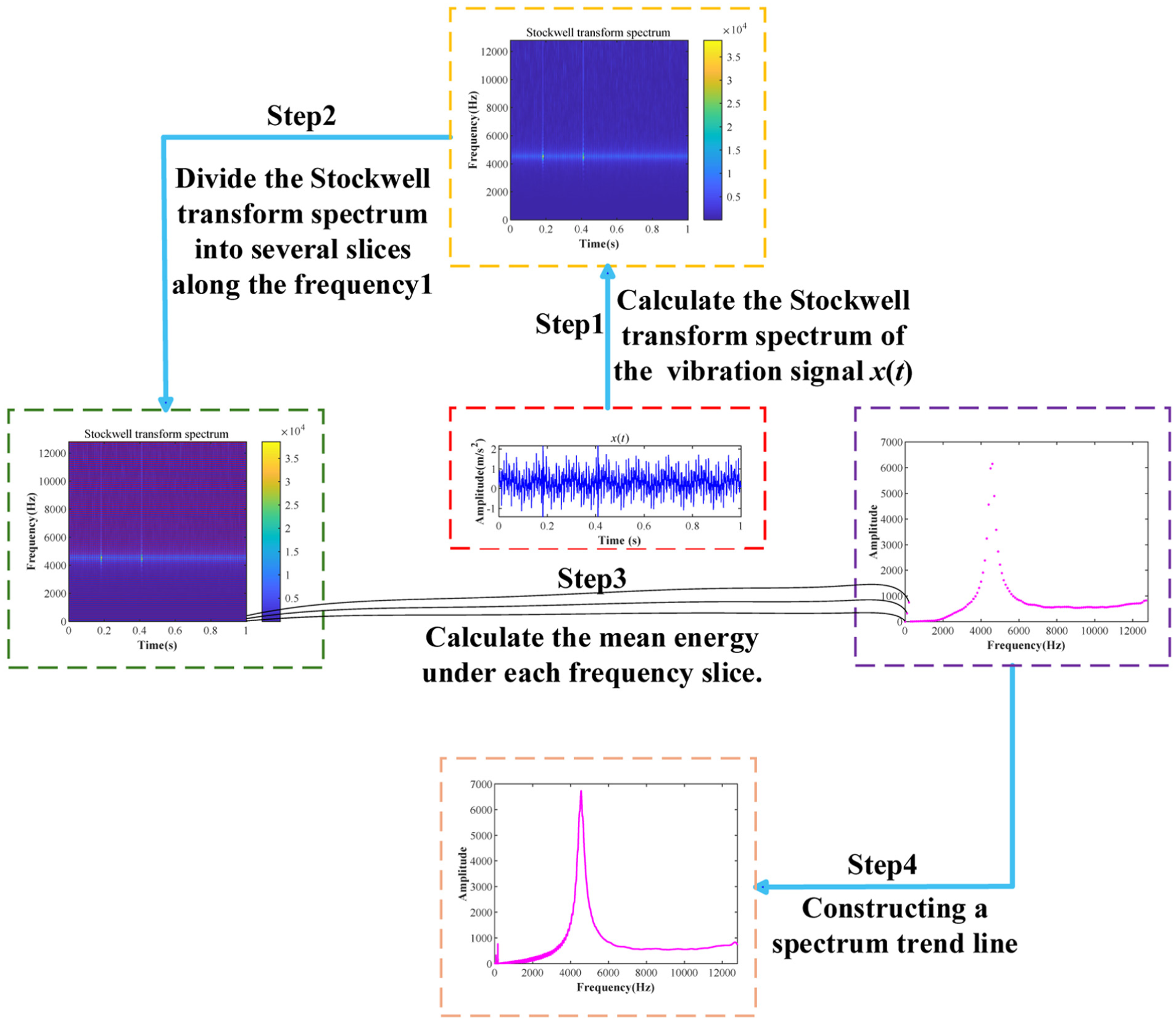
Simulation of the spectrum trend line construction process based on the ST spectrum. ST: Stockwell Transform.

Determination of the optimal spectral line and reconstruction of modal components

Although the spectral trend line can characterize the features of underlying fault information to some extent, the spectral segmentation boundaries often exhibit a dense distribution due to the interference of original noise. This increases the difficulty of accurately determining the segmentation boundaries. To address this, OSF is introduced in this paper to process the data within the window. This method effectively suppresses irrelevant frequency components and preserves the primary frequency components of high value under complex backgrounds. Specifically, by applying the OSF smoothing process with a window width W_OSF to the spectral trend line, a smooth trend line is extracted. Subsequently, all local minima of this trend line are identified and utilized as adaptive spectral segmentation boundaries. The entire frequency domain is then divided into several frequency bands. By combining the normalized boundaries within the [0, π] range with the endpoints 0 and π, an empirical wavelet filter bank with excellent attenuation performance is adaptively constructed to achieve the filtering of each band and the reconstruction of modal components. Finally, the specific steps for determining the optimal spectral line and the adaptive reconstruction of the empirical wavelet filter bank are illustrated in Figure 2, with the detailed steps described as follows:

Step 1: Calculate the spectral trend line and define the set of window widths as W_OSF1, W_OSF2, W_OSF _i , W_OSF _i+ ₁, W_OSF5, W_OSF6] = [0.5f_m, 1f_m, 1.5f_m, 2f_m, 2.5f_m, 3f_m]. Initialize the index i = 1.

According to research in reference 44, the window width W_OSF is a key parameter affecting the filtering performance. Considering the characteristics of rolling bearing faults, the search range in this paper is set to [0.5f_m, 3f_m], where f_m is the fault characteristic frequency, and the step size is 0.5f_m. The rationale for selecting the range of the window width W_OSF will be substantiated and discussed in detail in the “Simulation signal analysis and verification” section.

Step 2: Apply OSF smoothing to the spectral trend line using the window width W_OSF _i to obtain the ith smooth trend line SL(f) _i .

Step 3: Construct the adaptive empirical wavelet filter bank and reconstruct the modes. Based on the trend line SL(f) _i , construct an adaptive empirical wavelet filter bank to realize the reconstruction of modal components x_n(t), x_n(t) (where N is the total number of decomposed frequency bands). The specific steps are as follows:

1. Search for the local minima of the trend line SL(f) _i and use them as spectral segmentation boundaries. Sort these boundaries in ascending order to obtain the boundary set f_b = [f₁, f₂, f_n, …, f_N−1].

2. Map the boundary set f_b to the normalized frequency range [0,π] of the original signal x(t) to obtain the normalized boundary set w_b=[w₁, w₂,…,w_N−1]. By introducing the starting boundary w₀=0 and the terminal boundary w_N=π, the complete boundary set w_B is constructed.

3. Perform adaptive partitioning of the spectrum using the set w_b and construct the empirical wavelet filter bank using the set w_B. This yields the scale function ${\hat{ϕ}}_{λ} (w)$ and the wavelet function ${\hat{ψ}}_{n} (w)$ of the empirical wavelet. Their expressions are shown in Equations (4) and (5) respectively:

{\hat{ϕ}}_{w} (w) = {\begin{matrix} 1, if | w | \leq (1 - γ) w_{s}, \\ \cos [\frac{π}{2} β (\frac{1}{2 γ w_{s}} (| w | - (1 - γ) w_{s}))], \\ if (1 - γ) w_{s} \leq | w | \leq (1 + γ) w_{s}, \\ 0, otherwise . \end{matrix}

(4)

{\hat{ψ}}_{n} (w) = {\begin{matrix} 1, if (1 + γ) w_{n} \leq | w | \leq (1 - γ) w_{n + 1}, \\ \cos [\frac{π}{2} β (\frac{1}{2 γ w_{n}} (| w | - (1 - γ) w_{n}))], \\ if (1 - γ) w_{n} \leq | w | \leq (1 + γ) w_{n}, \\ \sin [\frac{π}{2} β (\frac{1}{2 γ w_{n}} (| w | - (1 - γ) w_{n}))], \\ if (1 - γ) w_{n + 1} \leq | w | \leq (1 + γ) w_{n + 1}, \\ 0, otherwise . \end{matrix}

(5)

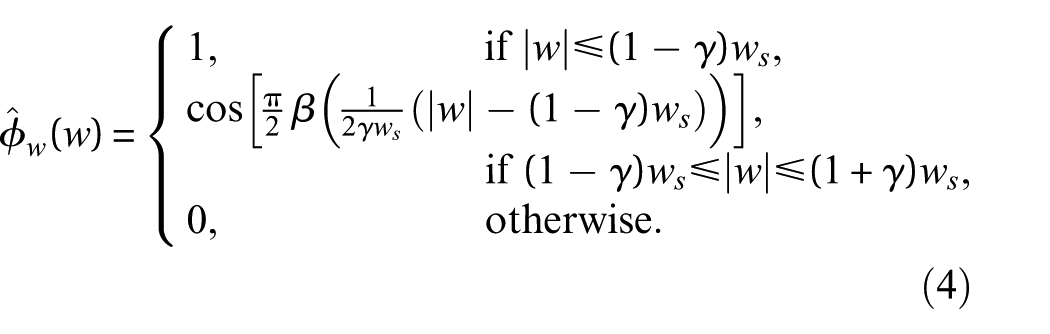
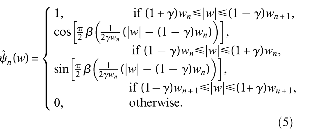
Where the transition function β(x) and the transition bandwidth τ_n are, respectively, defined as follows:

β (x) = x^{4} (35 - 84 x + 70 x^{2} - 20 x^{3})

(6)

τ_{n} = γ w_{n}, 0 < γ < 1

(7)

where the empirical wavelet filter bank constitutes a tight frame when $γ < min_{n} (\frac{w_{n + 1} - w_{n}}{w_{n + 1} + w_{n}})$ .

4. Use the constructed empirical wavelet filter bank to filter each partitioned frequency band, thereby reconstructing the various modal components x_n(t):

{\begin{matrix} x_{1} (t) = F^{- 1} ({\overset{\land}{W}}_{f} (0, w) \cdot {\overset{\land}{ϕ}}_{1} (w)) \\ x_{n} (t) = F^{- 1} ({\overset{\land}{W}}_{f} (n, w) \cdot {\overset{\land}{ψ}}_{n} (w)) \end{matrix}

(8)

Where F⁻¹ denotes the inverse Fourier transform, · represents the Fourier transform.

Step 4: Apply the OFCER indicator to perform a quantitative evaluation of the normalized envelope spectrum of each reconstructed modal component x_n(t). Calculate the OFCER _in value for each component, let max(OFCER _in ) = OFCER _i , and add it to the OFCER set.

Based on the studies by Lu et al.⁴⁵ and Yu et al.,⁴⁶ this paper proposes an optimized fault characteristic energy ratio (OFCER) indicator, which is formulated as follows:

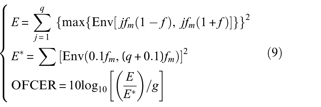
{\begin{matrix} E = \sum_{j = 1}^{q} {max {Env [j f_{m} (1 - f), j f_{m} (1 + f)]}}^{2} \\ E^{*} = \sum {[Env (0.1 f_{m}, (q + 0.1) f_{m})]}^{2} \\ OFCER = 10 \log_{10} [(\frac{E}{E^{*}}) / g] \end{matrix}

(9)

Where f_m denotes the fault characteristic frequency, q represents the number of harmonics, the frequency deviation value △f is 0.02, the gravity acceleration g is 9.8 × 10⁻³, Env(·) indicates the amplitude of the normalized envelope spectrum, E denotes the energy associated with fault characteristic information, and E* represents the total energy. From Equation (10), it can be seen that a larger OFCER value indicates a higher concentration of fault energy and a greater abundance of fault-related information.

Step 5: Determine if the loop index i satisfies i ≤ 5. If so, let i = i + 1 and return to step 1 through step 5; otherwise, proceed to step 6.

Step 6: From the set OFCER = [OFCER₁, OFC ER₂, OFCER _i , OFCER _i+ ₁, OFCER₅, OFCER₆], select the window width W_OSF _i corresponding to the maximum OFCER _i as the optimal window width W_OSF.

Step 7: Using the optimal window width W_OSF, execute step 2 through step 3 to obtain the optimal trend line SL(f) and the corresponding reconstructed modal components x_n(t).

Finally, Figure 3 presents a simulation diagram illustrating the construction of a set of empirical wavelet filter banks.

Figure 2.

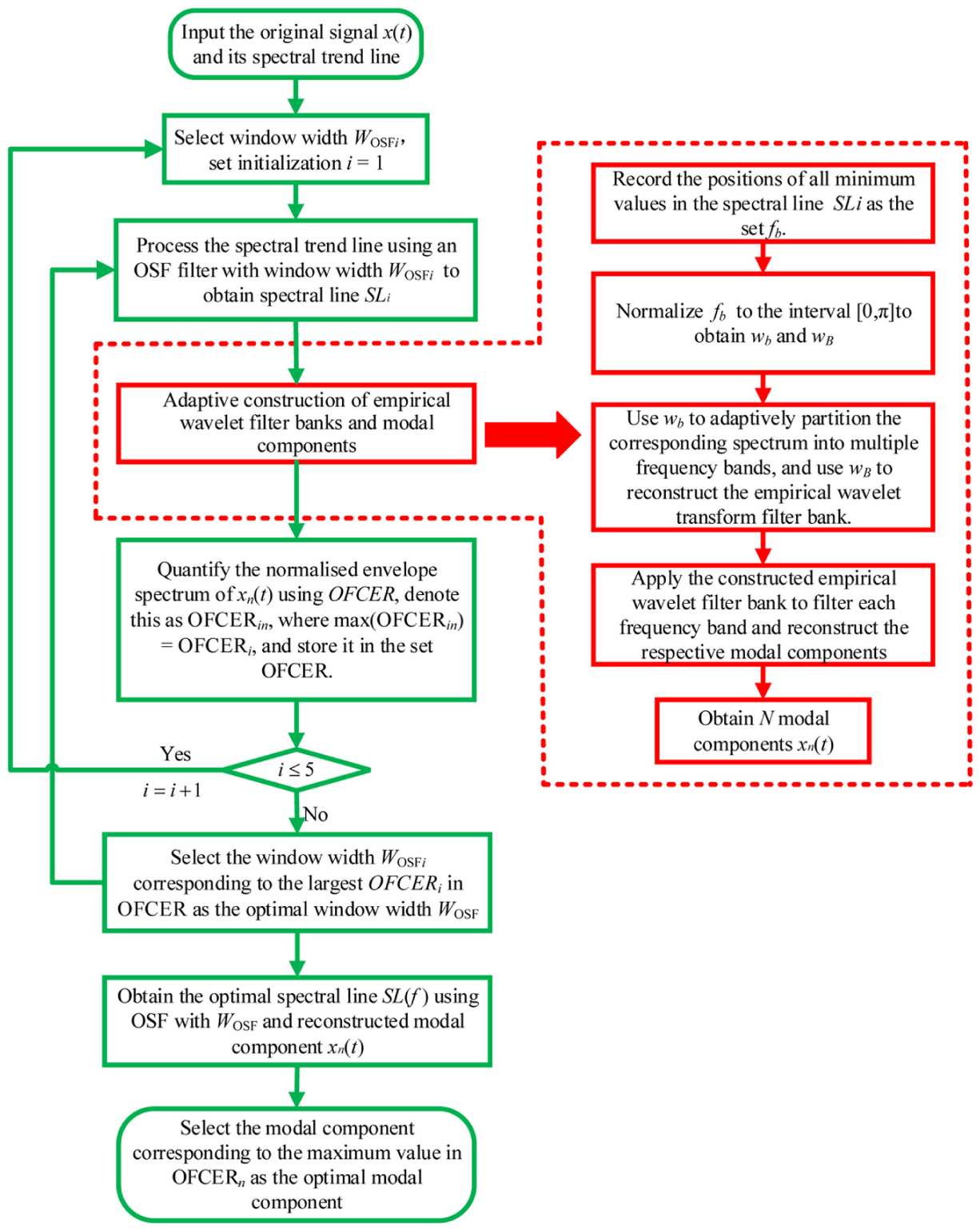
Flowchart for determining optimal spectral line and optimal modal component.

Figure 3.

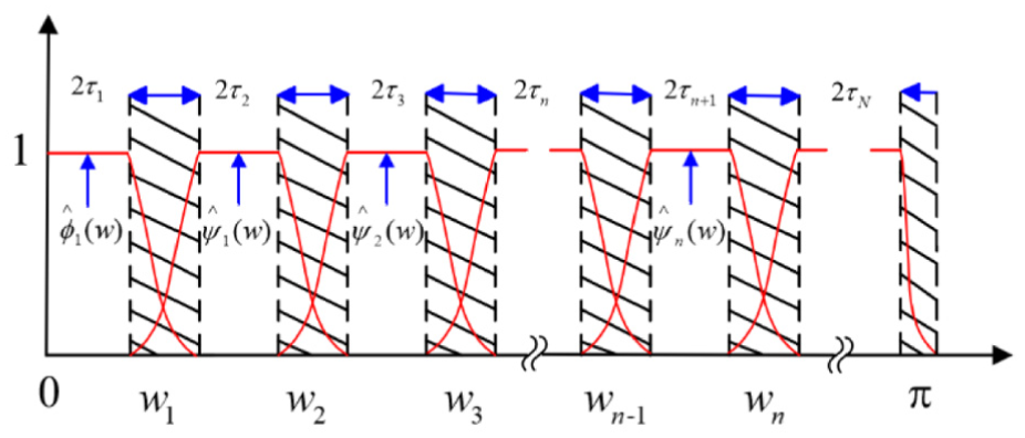
Simulation diagram of constructing a set of empirical wavelet filter banks.

Adaptive empirical wavelet filter banks

The flowchart illustrating a modal decomposition method of adaptively constructing empirical wavelet filter banks is shown in Figure 4. The steps are as follows:

Step 1: Apply the ST to the bearing vibration signal x(t) to obtain the corresponding time-frequency spectrum S(t, f).

Step 2: Calculate the average energy value Em_k of S(t, f) along the frequency axis to construct the spectral trend line.

Step 3: Select the window width W_OSF _i for OSF. Apply a smoothing moving average to the spectral trend line to obtain the filtered spectral line SL(f) _i , and initialize the index i = 1.

Step 4: Search for and record all local minima of the spectral line SL(f) _i to serve as the segmentation boundaries f_b.

Step 5: Construction of adaptive empirical wavelet filter banks and modal reconstruction. Construct the adaptive empirical wavelet filter bank based on SL(f) _i and perform modal reconstruction to obtain the reconstructed modal components x_n(t).

Step 6: Apply the OFCER indicator to perform a quantitative evaluation of the normalized envelope spectra of the N reconstructed modal components. Calculate the OFCER _in for each component. Meanwhile, let max(OFCER _in ) = OFCER _i and store it in the set OFCER.

Step 7: Determine whether the number of iterations satisfies i ≤ 5. If so, let i = i+1 and return to step 3 through step 6; otherwise, proceed to step 8.

Step 8: From the set OFCER = [OFCER₁, OFC ER₂, OFCER _i , OFCER _i+ ₁, OFCER₅, OFCER₆], select the window width W_OSF _i corresponding to the maximum value as the optimal window width W_OSF.

Step 9: Using the optimal window width W_OSF, execute step 3 through step 5 to obtain the optimal spectral line SL(f) and the corresponding reconstructed modal components x_n(t).

Step 10: Calculate the OFCER _n for each x_n(t), and select the modal component with the maximum indicator value as the optimal reconstructed modal component.

Step 11: Calculate the normalized envelope spectrum of the optimal modal component, extract the bearing fault characteristic frequency, and determine the fault type accordingly.

Figure 4.

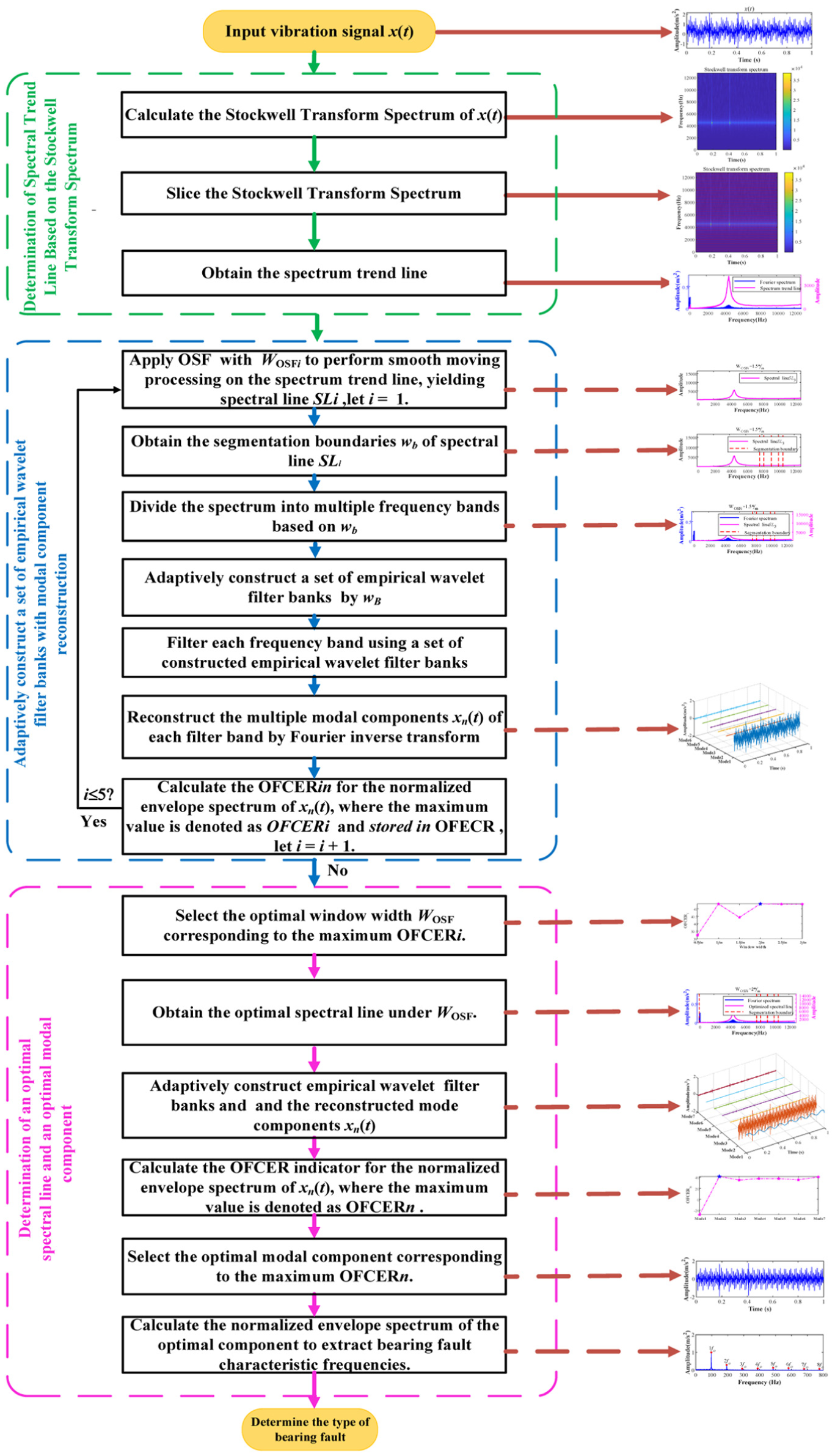
Overall flowchart of the proposed AEWFMD method. AEWFMD: adaptive empirical wavelet filter banks.

Simulated signal analysis and verification

Resonance band identification and noise reduction analysis for single fault signals

In this study, a spectral trend line based on the mean energy of frequency slices is constructed to characterize the energy distribution of various frequency components. It is observed that the local maxima of this mean energy typically correspond to potential fault resonance bands. Accordingly, an OSF is employed to smooth the spectral trend line, using its local minima as the boundaries for frequency band partitioning, thereby enabling the adaptive reconstruction of the empirical wavelet filter bank.

In summary, the noise reduction mechanism of the AEWFMD method consists of two stages: first, the pre-processing of the spectral trend line via an OSF filter; and second, the construction of empirical wavelet filters through precise resonance band boundary delimitation to facilitate the deep extraction of target fault components. To demonstrate the efficacy of the AEWFMD method in single resonance band identification and overall denoising performance, this section utilizes the rolling element bearing outer race fault simulation model shown in Equation (10)^47,48 for a systematic evaluation across three dimensions (3D).

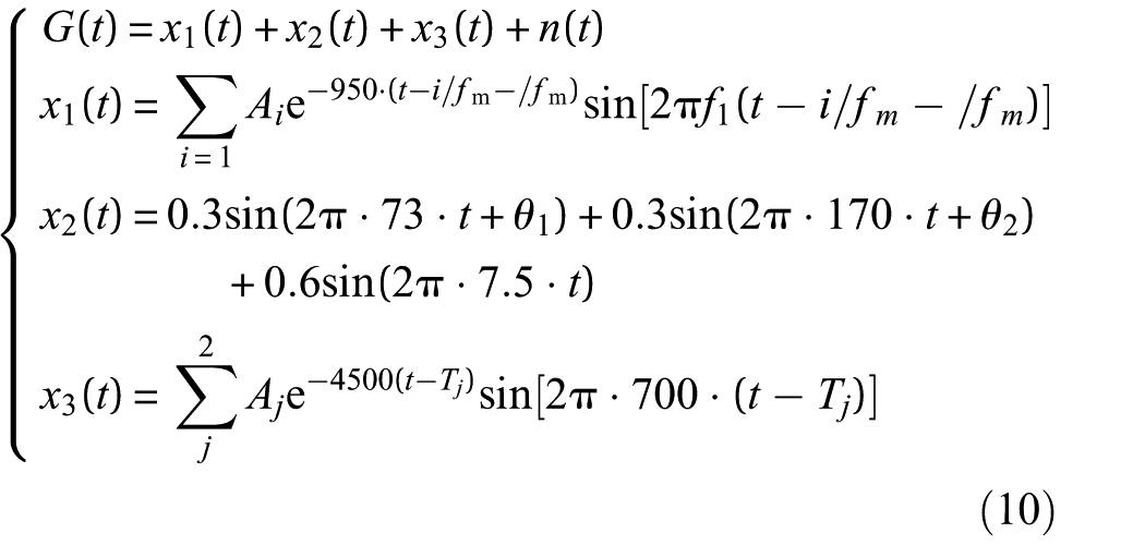
{\begin{matrix} G (t) = x_{1} (t) + x_{2} (t) + x_{3} (t) + n (t) \\ x_{1} (t) = \sum_{i = 1} A_{i} e^{- 950 \cdot (t - i / f_{m} - / f_{m})} \sin [2 π f_{1} (t - i / f_{m} - / f_{m})] \\ x_{2} (t) = 0.3 \sin (2 π \cdot 73 \cdot t + θ_{1}) + 0.3 \sin (2 π \cdot 170 \cdot t + θ_{2}) \\ + 0.6 \sin (2 π \cdot 7.5 \cdot t) \\ x_{3} (t) = \sum_{j}^{2} A_{j} e^{- 4500 (t - T_{j})} \sin [2 π \cdot 700 \cdot (t - T_{j})] \end{matrix}

(10)

Where x₁(t) simulates the periodic impulsive signals induced by an outer race fault, where A_i denotes the amplitude of the ith fault impulse, generated from a uniform distribution in the range [0.9,1]. The simulation parameters are set as follows: outer race fault characteristic frequency f_m, shaft rotation frequency f_r = 26 Hz, resonance frequency f₁ = 4450 Hz, and slippage rate Δ = 0.001. x₂(t) simulates the discrete harmonics generated by shaft rotation, with initial phases θ₁ and θ₂ set to π/6 and −π/3, respectively. x₃(t) represents impulsive interference caused by random transient shocks, where j denotes the occurrence time of the jth shock. The sampling frequency is set to 25.6 kHz with a total of 25,600 analysis points.

Dimension I: Analysis of frequency band partitioning and single resonance band extraction based on ST-spectrum energy distribution

First, the time-domain signal and the corresponding ST spectrum are presented for a bearing with an outer race fault (fault characteristic frequency f_m = 97 Hz. As illustrated in the time-frequency representation in Figure 5(b), a significant energy concentration is observed around 4450 Hz, indicating that the ST spectrum effectively captures the temporal distribution of fault information across different frequency components.

Figure 5.

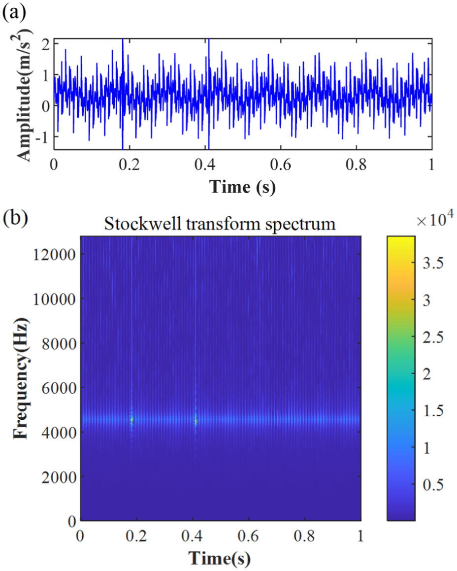
Time-domain waveform and its ST spectrum under f_m = 97 Hz and SNR = 0 dB: (a) time-domain waveform and (b) ST spectrum. ST: Stockwell Transform; SNR: signal-to-noise ratio.

Subsequently, a spectral trend line was constructed by calculating the mean energy of the ST spectrum along the frequency axis, as shown in Figure 6(a). The spectral trend line maintains high consistency with the overall profile of the raw spectrum, reaching a local maximum near 4450 Hz. This peak aligns closely with the preset fault resonance frequency, thereby validating the robustness and characterization accuracy of the proposed ST-based spectral trend line extraction method.

Figure 6.

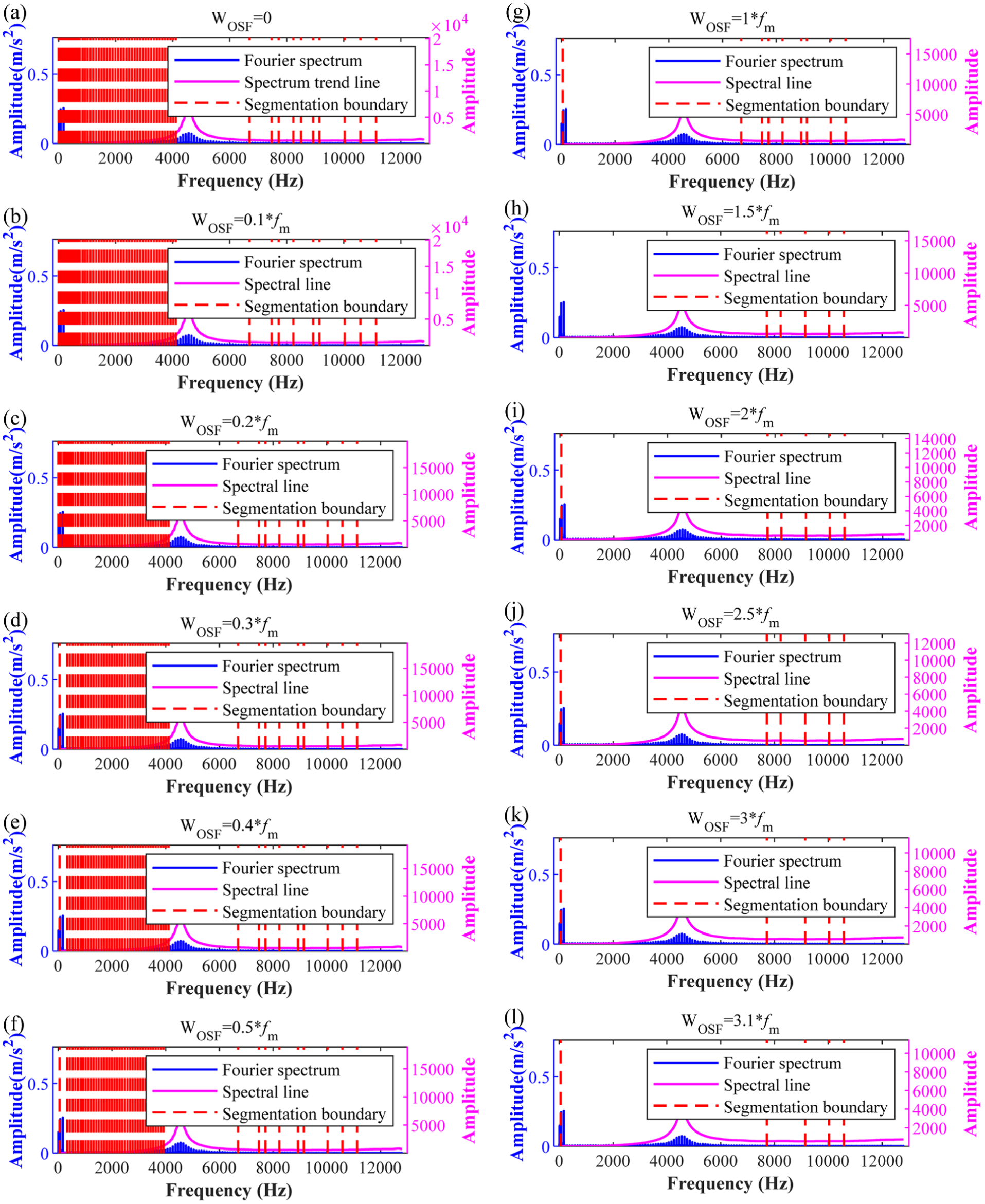
Spectral lines and spectral segmentation boundaries of AEWFMD under different window widths at f_m = 97 Hz and SNR = 0 dB: (a) window width W_OSF = 0, (b) window width W_OSF = 0.1f_m, (c) window width W_OSF = 0.2 f_m, (d) window width W_OSF = 0.3f_m, (e) window width W_OSF = 0.4f_m, (f) window width W_OSF = 0.5f_m, (g) window width W_OSF = 1f_m, (h) window width W_OSF = 1.5f_m, (i) window width W_OSF = 2f_m, (j) window width W_OSF = 2.5f_m, (k) window width W_OSF = 3f_m, and (l) window width W_OSF = 3.1f_m. AEWFMD: adaptive empirical wavelet filter banks; SNR: signal-to-noise ratio.

However, the initial segmentation boundaries derived directly from the spectral trend line are excessively dense, which hinders reasonable frequency band partitioning. To address this, an OSF with a window width W_OSF is applied to smooth the trend line. Figure 6(a) to (l) displays the segmentation boundaries for W_OSF values ranging across [0, 0.1f_m, 0.2f_m, 0.3f_m, 0.4f_m, 0.5f_m, 1f_m, 1.5f_m, 2f_m, 2.5f_m, 3f_m, 3.1f_m]. The results indicate that the number of boundaries is maximized at W_OSF = 0 and gradually decreases until reaching a stable state as W_OSF increases.

To further investigate the extraction capability of the AEWFMD method under varying noise intensities, Figure 7(a) to (d) illustrates the extracted boundaries adjacent to the resonance band under different window widths and noise levels (f_m = 97 Hz). It can be observed that the boundaries on both sides of the resonance band (marked in green) exhibit a bidirectional convergence toward the resonance frequency of 4450 Hz. This indicates that the proposed method is capable of accurately identifying the resonance bands.

Figure 7.

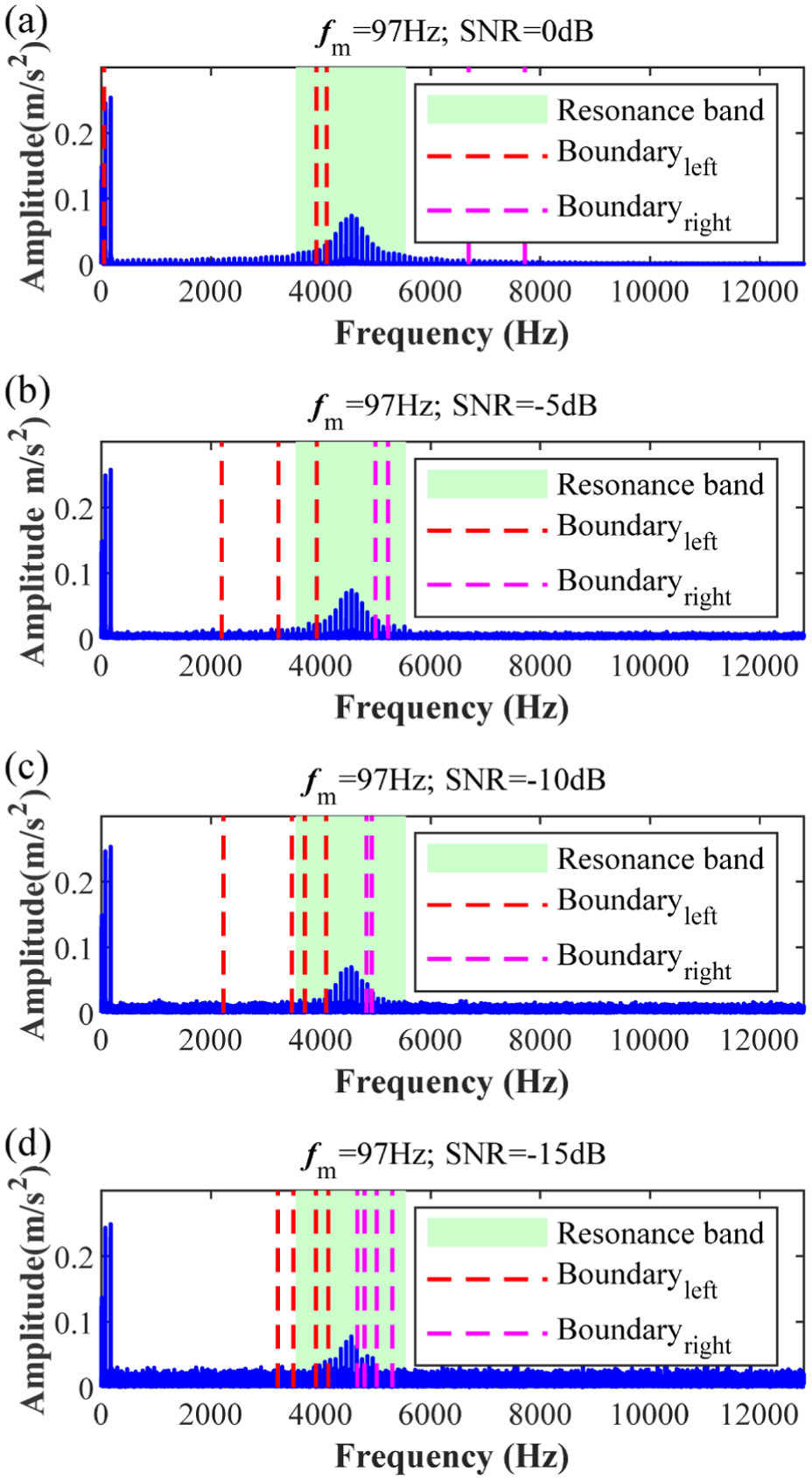
Adjacent boundaries (immediate left and right sides) of the resonance band for AEWFMD under various window widths and noise levels at f_m =97 Hz: (a) SNR = 0 dB, (b) SNR = −5 dB, (c) SNR = −10 dB, and (d) SNR = −15 dB. AEWFMD: adaptive empirical wavelet filter banks; SNR: signal-to-noise ratio.

Dimension II: Impact analysis of OSF filter window width W_OSF on filtering performance under various noise backgrounds

In this section, the number of segmentation boundaries and the OFCER are employed as quantitative evaluation metrics to investigate the influence of the OSF window width W_OSF on the smoothing effect of spectral trend lines. The objective is to verify the rationality and efficacy of the selected window range [0.5f_m, 3f_m].

Figure 8 illustrates the effects of varying window widths and signal-to-noise ratios (SNRs) on the number of segmentation boundaries and the optimal OFCER index at a fault characteristic frequency of f_m = 97 Hz. Analysis of the overall trends reveals that across different noise levels, as W_OSF increases, the optimal OFCER index initially increases monotonically, then gradually decreases, and finally stabilizes. Specifically:

1. In the interval W_OSF ∈ [0, 0.5f_m], the number of segmentation boundaries decreases sharply but remains relatively high, while the optimal OFCER index rises with the increasing window width.

2. Within the range W_OSF ∈ [0.5f_m, 3f_m], the decline in the number of boundary levels off, and the optimal OFCER index exhibits minimal fluctuation, demonstrating superior stability.

3. As W_OSF reaches 3.1f_m, both the number of boundaries and the OFCER index become nearly identical to those at W_OSF = 3f_m, indicating convergence.

Figure 8.

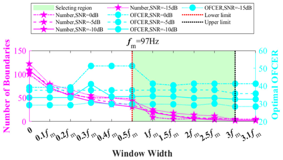
Number of division boundaries and optimal OFCER for the AEWFMD method under various window widths and SNR levels at f_m = 97 Hz. OFCER: optimized fault characteristic energy ratio; AEWFMD: adaptive empirical wavelet filter banks; SNR: signal-to-noise ratio.

Consequently, the interval [0.5f_m, 3f_m] is selected as the optimal range for W_OSF. The rationality of this choice lies in its ability to ensure reasonable boundary extraction while effectively reducing the number of iterations required to search for the optimal modal components. This further validates the scientific merit of using OSF for the moving average processing of spectral trend lines; the method significantly curtails redundant boundaries while ensuring that the optimal mode is captured within the specified window range. Furthermore, the high consistency of the trends across various noise intensities underscores the effectiveness of the selected window range and the excellent denoising performance of the OSF filter.

To further explore the potential impact of different fault characteristic frequencies f_m on filtering performance, the influence of OSF window width on spectral trend line extraction was analyzed under both noise-free and strong-noise conditions. Figure 9 presents the results for 50, 97, 124, and 178 Hz. The simulation data indicate that the evolution of the optimal OFCER index with respect to W_OSF is highly consistent regardless of the SNR or the magnitude of f_m. Notably, in the range W_OSF in [0.5f_m, 3f_m], the experimental curves overlap significantly, suggesting that the value of f_m has a negligible effect on the OSF filtering performance. This conclusion reaffirms the theoretical and practical universality of using [0.5f_m, 3f_m] as the predefined range for W_OSF.

Figure 9.

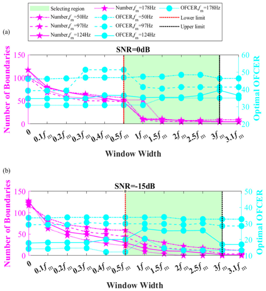
Number of division boundaries and optimal OFCER for AEWFMD under various window widths and fault characteristic frequencies f_m at a constant SNR: (a) SNR = 0 dB and (b) SNR = −15 dB. OFCER: optimized fault characteristic energy ratio; AEWFMD: adaptive empirical wavelet filter banks; SNR: signal-to-noise ratio.

Dimension III: Performance evaluation of filter banks based on resonance band division boundary for single fault signals

To evaluate the performance of the empirical wavelet filter bank constructed via resonance band boundary partitioning in the AEWFMD method, this section provides an in-depth analysis of its feature extraction capability under strong background noise.

Specifically, a simulation test was conducted using a high-noise signal with a fault characteristic frequency f_m = 97 Hz and SNR of −15 dB. Based on the previous analytical conclusions, the OSF filter window width was set to W_OSF = 2.5f_m. Figure 10 presents the 3D waterfall plot of the time-domain modal components (modes 1–13) reconstructed by the AEWFMD method.

Figure 10.

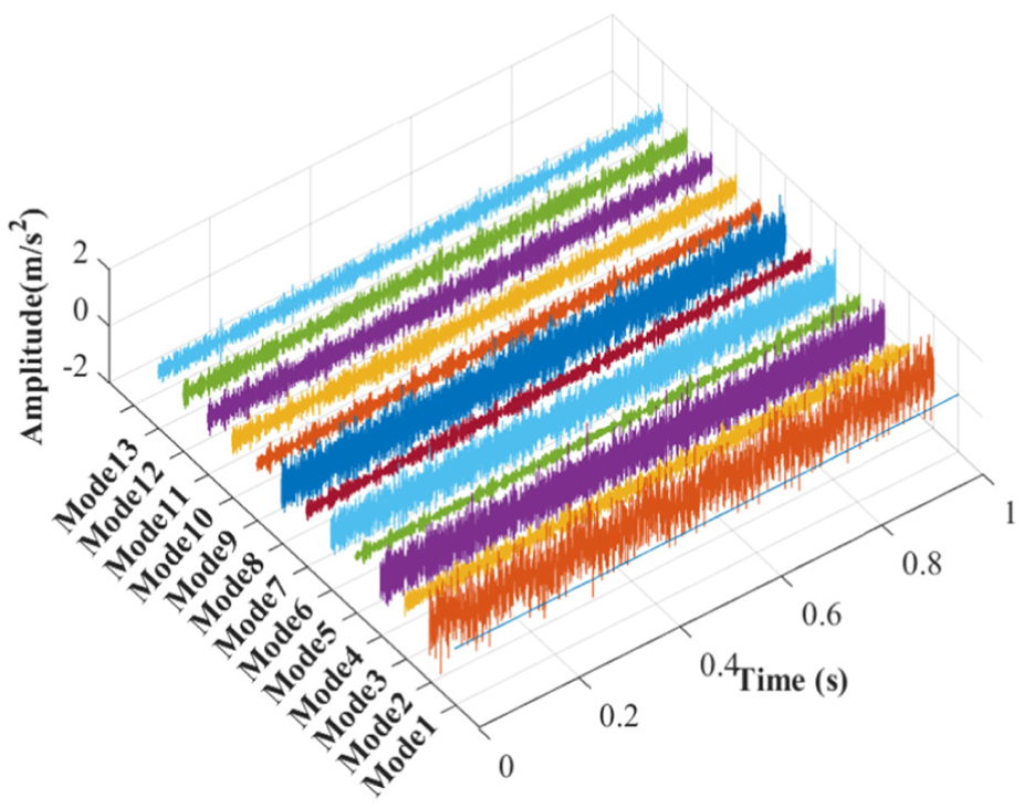
Reconstructed time-domain modal components of AEWFMD at f_m = 97 Hz and SNR = −15 dB. AEWFMD: adaptive empirical wavelet filter banks; SNR: signal-to-noise ratio.

Furthermore, the distribution of OFCER indices across all modal components in Figure 11 reveals that mode 4 achieves the maximum value, with mode 2 following closely behind. By performing envelope spectrum analysis on mode 4, as shown in Figure 12, multi-order fault characteristic frequencies from 1f_m to 8f_m can be clearly identified. These results demonstrate that the proposed OFCER index can accurately determine the optimal modal component within the signal, thereby providing robust evidence for the effectiveness of the AEWFMD method in extracting fault features under intense noise interference.

Figure 11.

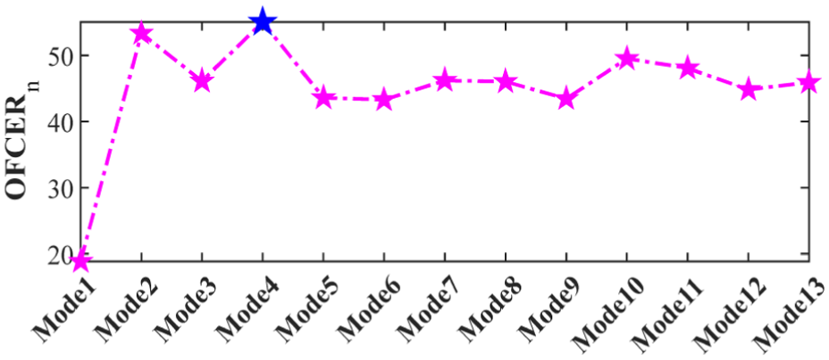
OFCER indicator values for each reconstructed time-domain modal component at f_m = 97 Hz and SNR = −15 dB. OFCER: optimized fault characteristic energy ratio; SNR: signal-to-noise ratio.

Figure 12.

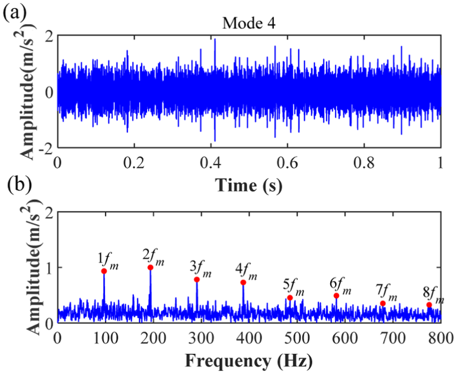
The time-domain waveform of mode 4 and its normalized envelope spectrum at f_m = 97 Hz and SNR = −15 dB: (a) time-domain waveform and (b) normalized envelope spectrum. SNR: signal-to-noise ratio.

Resonance band identification and noise reduction analysis for compound fault signals

To elucidate the resonance band separation and identification mechanism of the AEWFMD method, as well as its overall denoising performance in compound fault diagnosis, a rolling element bearing compound fault signal is constructed as shown in Equation (11), building upon the single-fault model in Equation (10).^49,50 Its effectiveness is systematically validated across 3D.

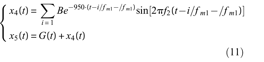
{\begin{matrix} x_{4} (t) = \sum_{i = 1} B e^{- 950 \cdot (t - i / f_{m 1} - / f_{m 1})} \sin [2 π f_{2} (t - i / f_{m 1} - / f_{m 1})] \\ x_{5} (t) = G (t) + x_{4} (t) \end{matrix}

(11)

In Equation (11), x₄(t) simulates the periodic impulsive signals induced by an inner race fault. The amplitude modulation coefficient is defined as B = C_B (1−sin(2πf_rt), with C_B = 0.5. The specific simulation parameters are configured as follows: the inner race fault characteristic frequency f_m1 is 142 Hz, the shaft rotation frequency f_r is 26 Hz, and the resonance frequency f₂ is 8450 Hz. Furthermore, x₅(t) represents the resulting compound bearing fault signal. In this study, the sampling frequency is set to 25.6 kHz, and the number of analysis points is 25,600.

Dimension I: Separation and extraction analysis of compound fault resonance bands based on ST-spectrum energy distribution

To further investigate the capability of the AEWFMD method in separating and extracting resonance bands from compound faults under strong noise interference, a series of simulation experiments were conducted. Figure 13(a) to (d) illustrates the frequency band partitioning results for a compound fault signal containing an outer race fault characteristic frequency (f_o=97 Hz) and an inner race fault characteristic frequency (f_i = 142 Hz) under varying OSF window widths and SNRs.

Figure 13.

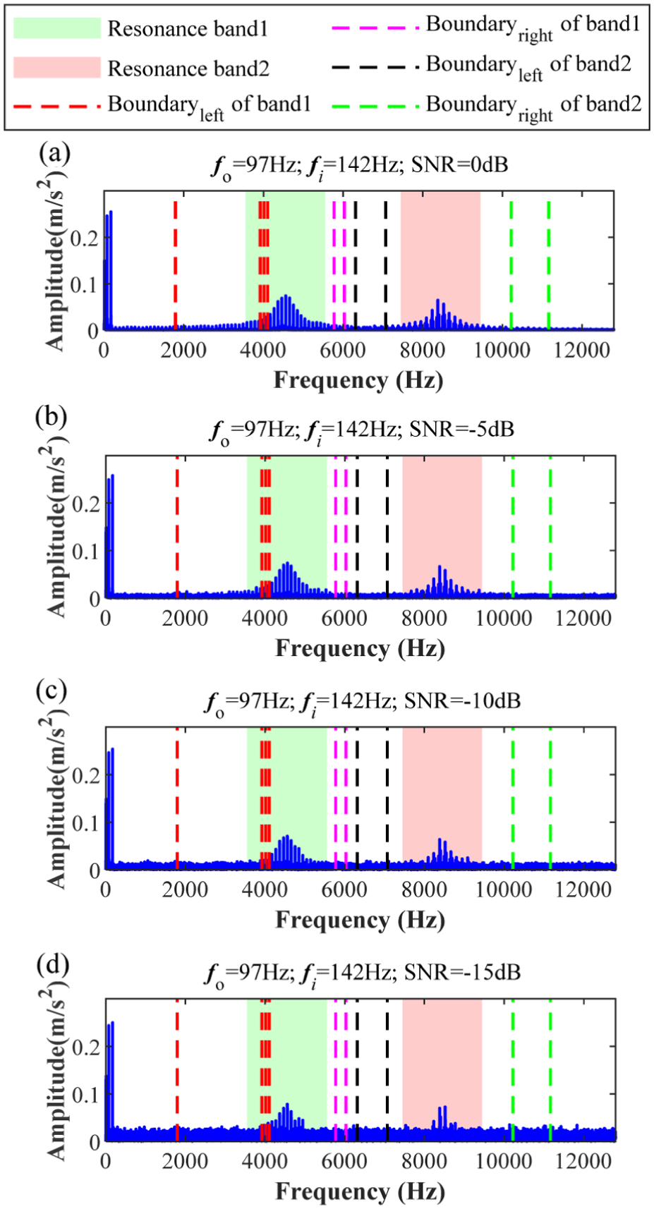
Adjacent boundaries (immediate left and right sides) of the resonance band for AEWFMD under various window widths and noise levels at f_o = 97 Hz and f_i = 142 Hz: (a) SNR = 0 dB, (b) SNR = −5 dB, (c) SNR = −10 dB, and (d) SNR = −15 dB. AEWFMD: adaptive empirical wavelet filter banks; SNR: signal-to-noise ratio.

The analysis of the illustrated results reveals that the boundaries of the resonance band indicated by the green-marked region accurately exhibit a bidirectional convergence toward the outer race fault resonance frequency (f₁ = 4450 Hz). Concurrently, the boundaries of the resonance band shown in the pink-marked region achieve a similar bidirectional approach toward the inner race fault resonance frequency (f₂ = 8450 Hz). These simulation results demonstrate that the AEWFMD method can effectively achieve the precise separation and identification of two distinct resonance bands within a compound fault, thereby validating its efficacy and robustness in the decomposition of complex composite signals.

Dimension II: Impact analysis of OSF filter window width W_OSF on filtering performance for multi-noise compound fault signals

Using the number of segmentation boundaries and the OFCER index as quantitative evaluation criteria, this section investigates the influence of the OSF window width W_OSF on the spectral trend line smoothing of compound fault signals under intense background noise. The goal is to verify the rationality and universality of the predefined window set W_OSF _i ∈ [0.5f_m, 1f_m, 1.5f_m, 2f_m, 2.5f_m, 3f_m].

Figure 14(a) and (b) presents the boundary counts and optimal OFCER results under various window widths and SNRs for f_m = f_o = 97 Hz and f_m = f_i = 142 Hz, respectively. Overall, across different SNR levels, the optimal OFCER index exhibits an initial upward trend followed by a gradual decrease, eventually stabilizing as W_OSF increases. This evolution confirms the scientific merit of employing OSF for the moving average processing of spectral trend lines, as it simultaneously curtails redundant boundaries and ensures the capture of the optimal modal components within a specific W_OSF range. Furthermore, the consistent trends in boundary counts and OFCER values across various noise intensities demonstrate the superior denoising performance of the OSF filter, reaffirming that the interval [0.5f_m, 3f_m] remains a valid and effective range for compound fault decomposition.

Figure 14.

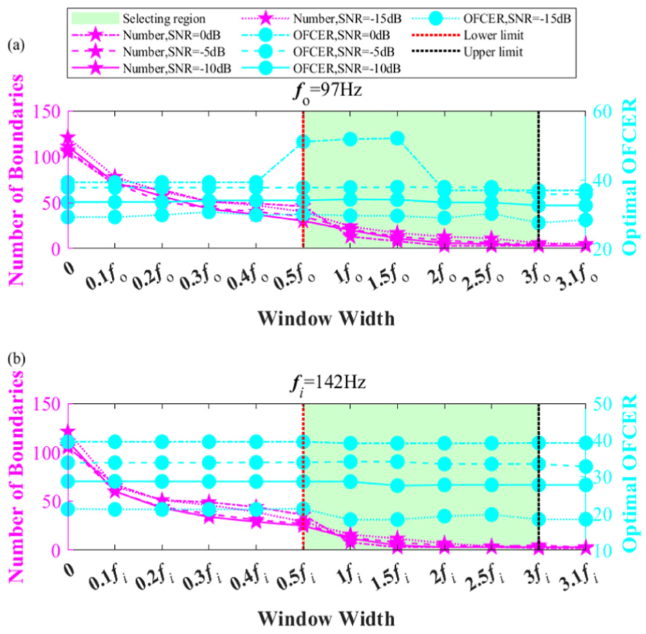
Number of division boundaries and optimal OFCER for the AEWFMD method under various window widths and SNR levels at f_o = 97 Hz or f_i = 142 Hz: (a) f_o = 97 Hz and (b) f_i = 142 Hz. OFCER: optimized fault characteristic energy ratio; AEWFMD: adaptive empirical wavelet filter banks; SNR: signal-to-noise ratio.

Dimension III: Performance evaluation of filter banks based on resonance band division boundary for compound fault signals

To validate the filtering performance of the empirical wavelet filter bank within the AEWFMD framework, the capability to extract compound fault features under extreme background noise is explored. The experimental setup and analysis are as follows:

First, the decomposition was performed on a high-noise composite signal (SNR = −15 dB) containing both an outer race fault (f_o = 97 Hz) and an inner race fault (f_i = 142 Hz). By setting f_m = f_o = 97 Hz, the AEWFMD method was applied to the signal. Figure 15 displays the 3D waterfall plot of the reconstructed modal components (modes 1–12) with W_OSF =2.5f_m. As shown in the OFCER distribution in Figure 16, mode 3 achieves the maximum index value. Its envelope spectrum in Figure 17 clearly reveals the outer race fault characteristic frequencies from 1f_o to 5f_o.

Figure 15.

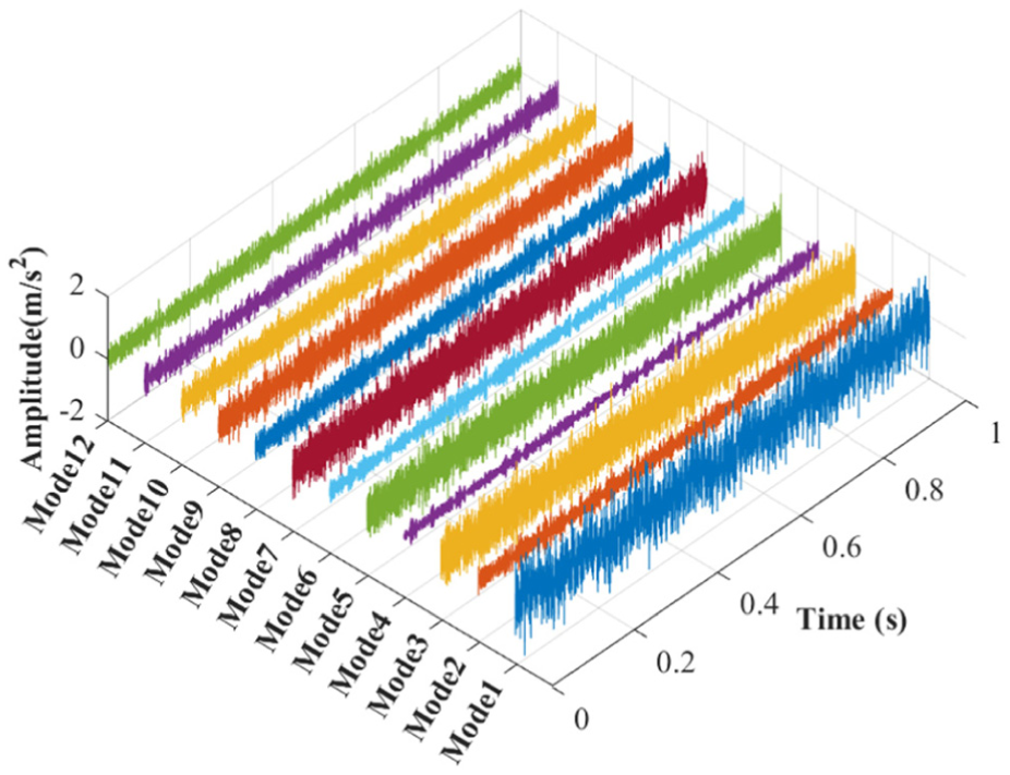
Reconstructed time-domain modal components of AEWFMD at f_o = 97 Hz and SNR = −15 dB. AEWFMD: adaptive empirical wavelet filter banks; SNR: signal-to-noise ratio.

Figure 16.

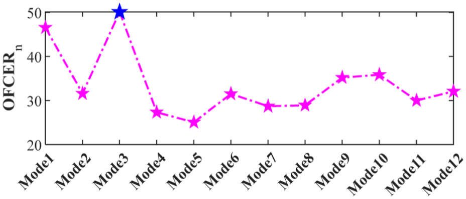
OFCER indicator values for each reconstructed time-domain modal component at f_o = 97 Hz and SNR = −15 dB. OFCER: optimized fault characteristic energy ratio; SNR: signal-to-noise ratio.

Figure 17.

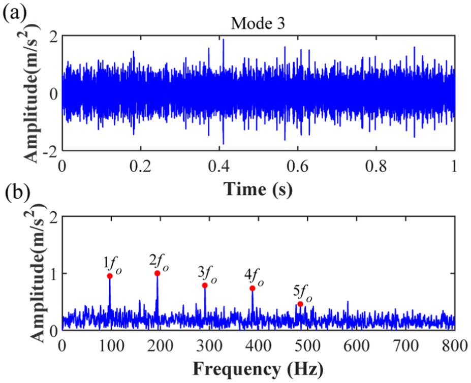
The time-domain waveform of mode 3 and its normalized envelope spectrum at f_o = 97 Hz and SNR = −15 dB: (a) time-domain waveform and (b) normalized envelope spectrum. SNR: signal-to-noise ratio.

Subsequently, the same composite signal is decomposed by setting f_m = f_i = 142 Hz. As illustrated in Figure 18, mode 23 exhibits the highest OFCER index. In the corresponding envelope spectrum (Figure 19), the inner race fault characteristic frequencies from 1f_i to 3f_i are accurately identified. In summary, these findings demonstrate that the AEWFMD method is highly effective in separating and extracting compound fault signatures.

Figure 18.

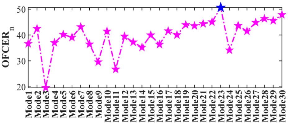
OFCER indicator values for each reconstructed time-domain modal component at f_i = 142 Hz and SNR = −15 dB. OFCER: optimized fault characteristic energy ratio; SNR: signal-to-noise ratio.

Figure 19.

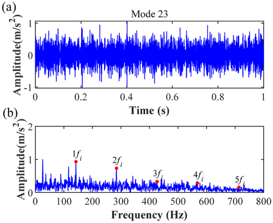
The time-domain waveform of mode 23 and its normalized envelope spectrum at f_i = 142 Hz and SNR = −15 dB: (a) time-domain waveform and (b) normalized envelope spectrum. SNR: signal-to-noise ratio.

Experimental signal analysis and verification

To evaluate the practical effectiveness of the proposed AEWFMD method, this section implements it across various bearing fault diagnosis scenarios. Specifically, the analysis utilizes the full life-cycle outer race fault data from the NSF I/UCR Center, rolling element fault data from high-speed train axle boxes, and compound fault data provided by the Hanoi University of Science and Technology (HUST). Furthermore, comparative studies involving EWT, EFD, and FMD methods are conducted to demonstrate the superiority of the proposed AEWFMD approach in feature extraction and diagnostic accuracy.

Case 1: Application in natural outer race fault diagnosis

To further validate the effectiveness of the AEWFMD method in detecting outer race defects, this section utilizes the run-to-failure bearing dataset provided by the Center for Intelligent Maintenance Systems (IMS).⁵¹ The experimental setup, illustrated in Figure 20, consists of an AC motor operating at a constant speed of 2000 r/min, which drives a shaft via a friction belt. Four bearings (specifications listed in Table 1) are mounted on the shaft and subjected to a radial load of 26.7 kN exerted by a spring mechanism.

Figure 20.

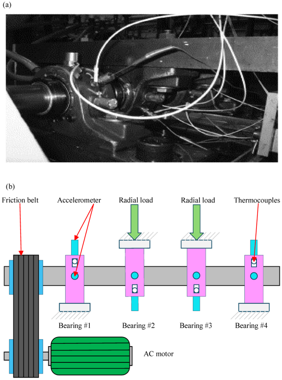
Intelligent maintenance simulated fault test bench and structural distribution diagram: (a) intelligent maintenance simulated fault test bench and (b) structural distribution diagram.⁵¹

Table 1.

The geometric parameters of the outer ring bearing with fault in case 1.

Pitch diameter (mm)	Ball diameter (mm)	Number of rollers	Contact angle
71.501	8.407	16	15.17°

Vibration signals were acquired using PCB 353 B33 accelerometers and a DAQ 6062 E data acquisition system. The sampling frequency was set to 20 kHz with a sampling interval of 10 min. A total of 984 data segments were collected over a span of 164 h. For this analysis, the data captured at the 423 min, which corresponds to the incipient fault stage, was selected.⁵² The theoretical fault characteristic frequency of the outer race, f_o, is approximately 230 Hz.

Figure 21 presents the time-domain waveform and the corresponding envelope spectrum of the selected vibration signal. As illustrated in Figure 21(a), the periodic impulsive features indicative of a fault are completely masked by heavy background noise and other interfering components. Consequently, the characteristic frequency of the outer race fault, 1f_o, is indistinguishable in the envelope spectrum shown in Figure 21(b). These observations suggest that the bearing is in an incipient fault stage, where conventional diagnostic methods fail to effectively identify the presence and type of rolling element bearing defects.

Figure 21.

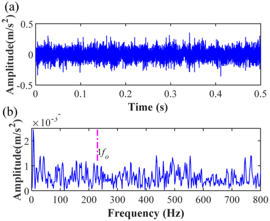
Time waveform and envelope spectrum of outer ring fault signal under case 1: (a) time waveform and (b) envelope spectrum.

First, the proposed AEWFMD method is employed for feature extraction from the outer race fault signal. Initially, the ST spectrum (Figure 22) is calculated, followed by the construction of a spectral trend line based on the energy mean values. By setting the reference frequency f_m = f_o, various window widths W_OSF are selected from the set [0.5f_m, 1f_m, 1.5f_m, 2f_m, 2.5f_m, 3f_m] to perform OSF filtering on the spectral energy lines, yielding a series of smoothed curves. Furthermore, the maximum ORCER values for each mode component across different spectral lines are computed and recorded. It is observed that the ORCER reaches its peak value of 17.4579 when the window width W_OSF is 0.5f_m. The resulting optimal spectral line, represented by the purple curve in Figure 23, shows high consistency with the overall spectral trend. Subsequently, all local minima of this optimal line are identified as segmentation boundaries (indicated by red dashed lines in Figure 23) to adaptively partition the spectrum into multiple frequency bands.

Figure 22.

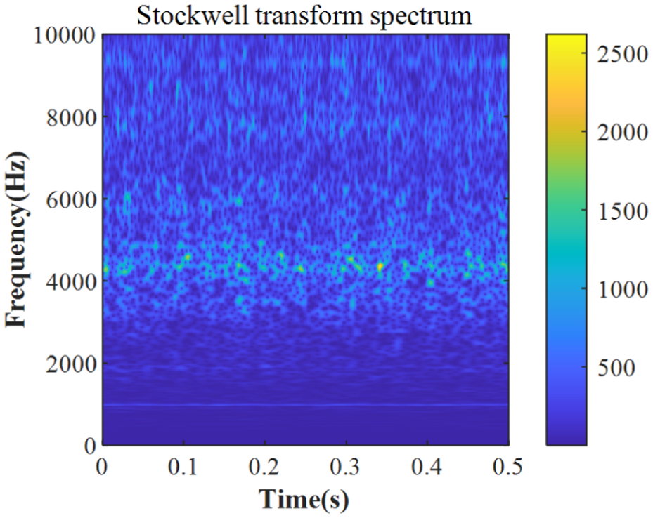
ST spectrum under case 1. ST: Stockwell Transform.

Figure 23.

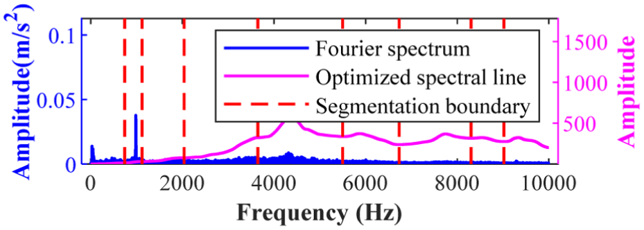
Optimal spectral line and segmentation boundaries of AEWFMD under case 1. AEWFMD: adaptive empirical wavelet filter banks.

On this basis, an empirical wavelet filter bank is constructed according to these boundaries to filter the signal, adaptively reconstructing nine modal components, denoted as modes 1–9 (Figure 24). This process demonstrates that the AEWFMD method eliminates the need for prior knowledge regarding the number of modes, enabling an autonomous and rational partitioning of the spectrum and reconstruction of modal components. Subsequently, the OFCER index is employed to quantitatively evaluate the performance of mode 1 through mode 9 (Figure 25). The results indicate that mode 7 yields the maximum OFCER value (highlighted in blue), identifying it as the optimal modal component containing the most salient fault information. Finally, the time-domain waveform and normalized envelope spectrum of mode 7 are presented in Figure 26. As illustrated in Figure 26(b), the outer race fault characteristic frequency 1f_o and its second harmonic 2f_o are clearly identifiable, with interfering noise being effectively suppressed. These diagnostic findings are highly consistent with the actual bearing condition, thereby validating the effectiveness and practical applicability of the proposed AEWFMD method in extracting incipient fault features.

Figure 24.

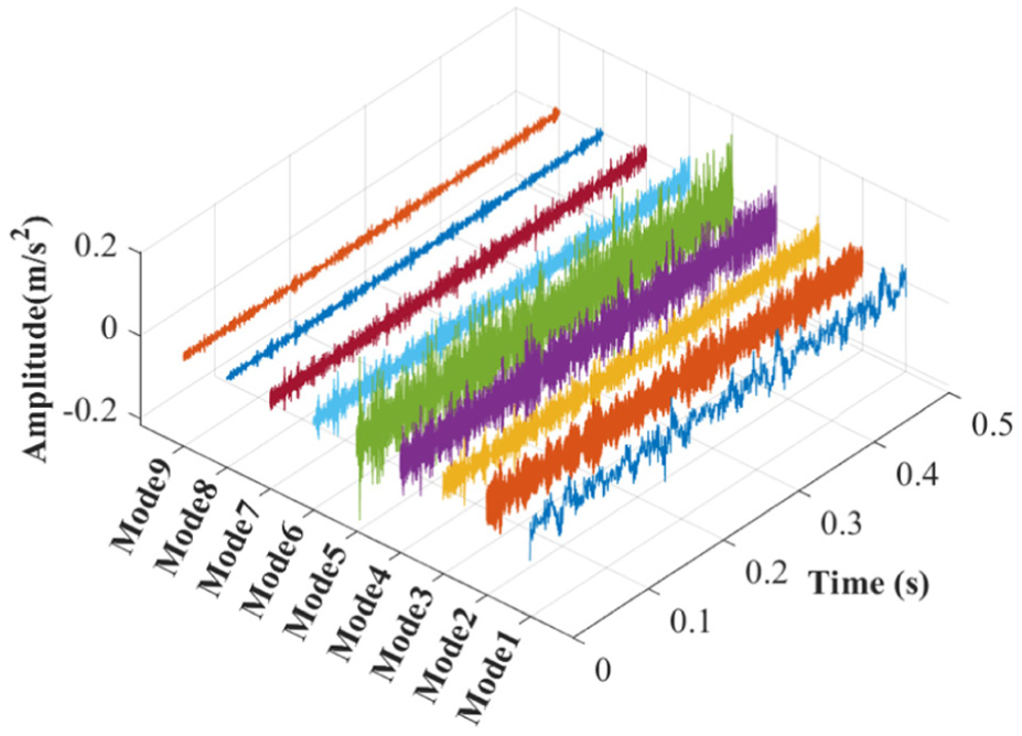
The reconstructed time-domain modal components of AEWFMD under case 1. AEWFMD: adaptive empirical wavelet filter banks.

Figure 25.

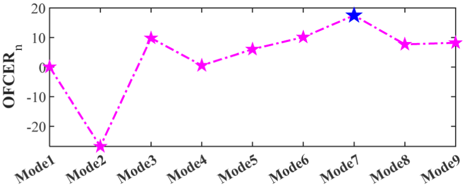
OFCER indicator values for each reconstructed time-domain modal component under case 1. OFCER: optimized fault characteristic energy ratio.

Figure 26.

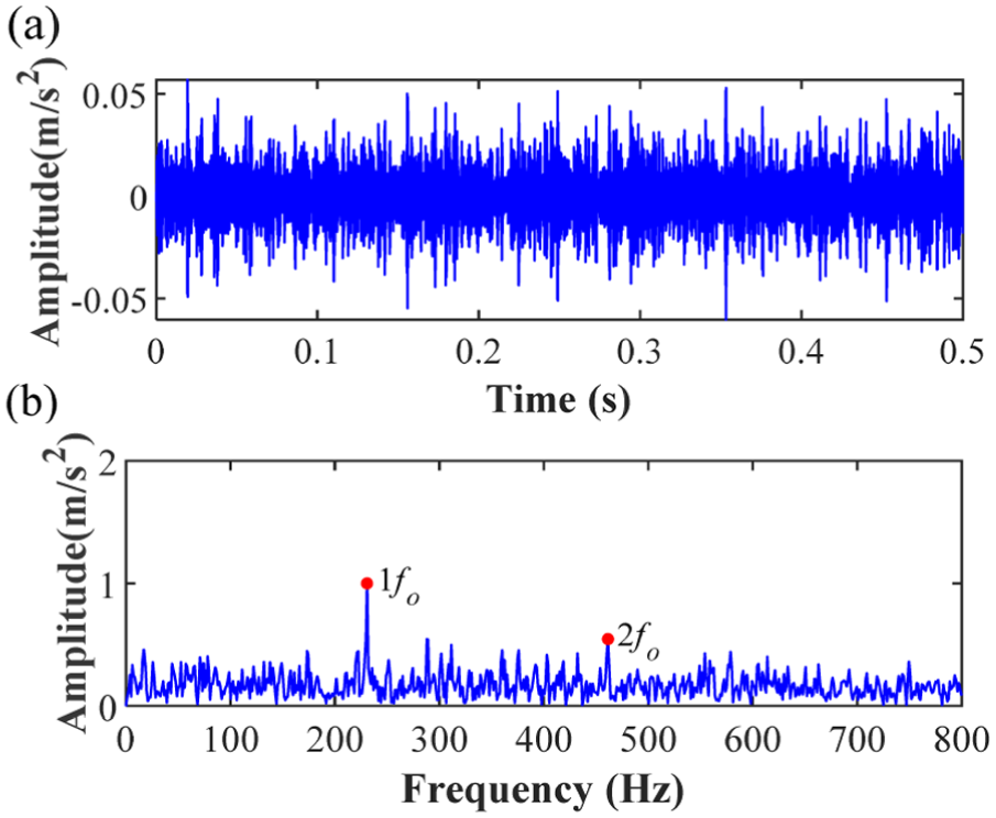
The time-domain waveform of mode 7 and its normalized envelope spectrum under case 1: (a) time-domain waveform and (b) normalized envelope spectrum.

Secondly, to evaluate the comparative performance, the EWT method is implemented with the number of decomposition modes preset to 9 to extract features from the outer race fault signal. Figure 27 illustrates the spectral segmentation boundaries generated by the EWT method. As shown in Figure 27(a), a high density of segmentation boundaries is observed around 50 and 1000 Hz. Specifically, the enlarged view in Figure 27(b) reveals three closely spaced boundaries near 50 Hz and two near 1000 Hz. Such redundant partitioning leads to spectral over-decomposition, which potentially triggers the generation of irrelevant or spurious components. Subsequently, the reconstructed modal components (modes 1–9) and their corresponding normalized envelope spectra are presented in Figure 28. Finally, it is observed from Figure 28(b) that only a faint trace of the outer race fault characteristic frequency 1f_o is identifiable in the envelope spectrum of mode 7, making it difficult to accurately determine the bearing fault type.

Figure 27.

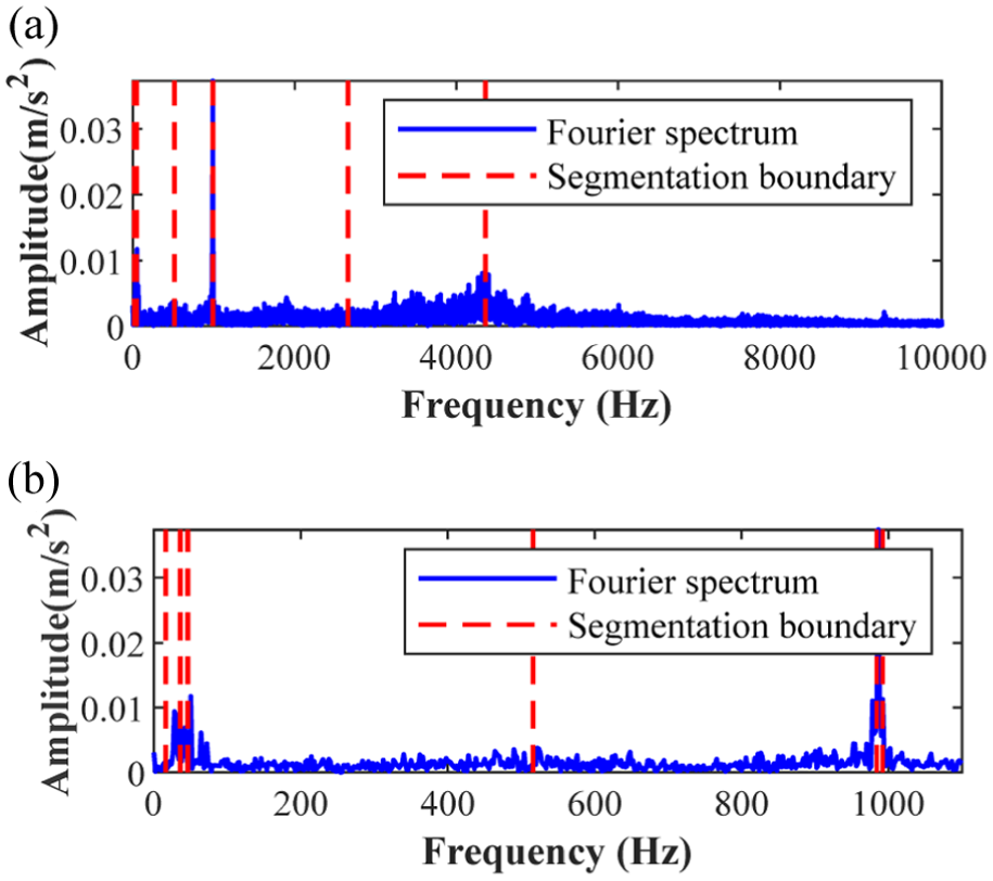
Spectrum segmentation boundaries of EWT under case 1: (a) segmentation boundaries and (b) enlarged view of the spectrum segmentation boundaries. EWT: empirical wavelet transform.

Figure 28.

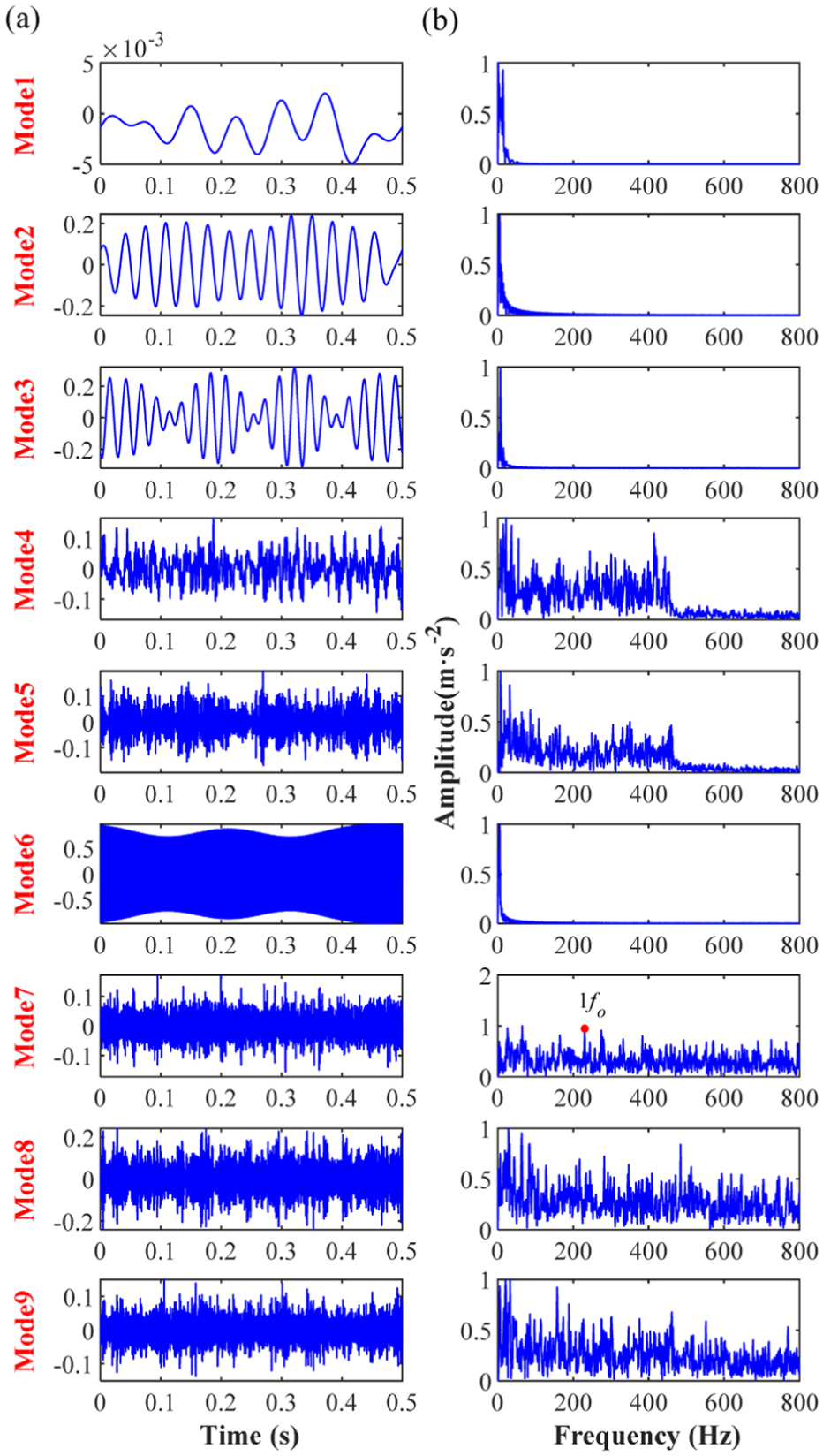
The reconstructed time-domain modal components and normalized envelope spectrum of EWT under case 1: (a) time-domain waveform and (b) normalized envelope spectrum. EWT: empirical wavelet transform.

Subsequently, the EFD method was employed as a second comparative approach, with the decomposition mode count preset to 9. Figure 29 illustrates the spectral segmentation boundaries determined by the EFD method for the outer race fault signal. As shown in Figure 29(a), a noticeable clustering of segmentation boundaries is observed around 0, 1000, and 4300 Hz. Specifically, the enlarged view in Figure 29(b) clarifies that three closely spaced boundaries exist near 0 Hz, while two redundant boundaries appear near both 1000 and 4300 Hz.This improper partitioning results in severe spectral over-decomposition. Compared to the AEWFMD results in Figure 23, both EFD and EWT suffer from excessively dense segmentation. Figure 30 presents the reconstructed modes (modes 1–9) and their corresponding normalized envelope spectra. As illustrated in Figure 30(b), only a faint trace of the characteristic frequency 1f_o can be identified in the envelope spectrum of mode 9. The persistent noise interference prevents a definitive diagnosis, making it difficult to accurately identify the bearing fault type using the EFD method.

Figure 29.

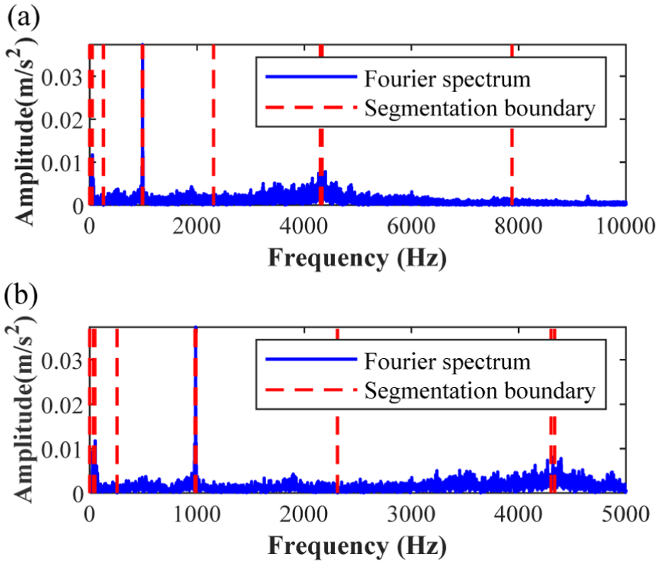
Spectrum segmentation boundaries of EFD under case 1: (a) segmentation boundaries and (b) enlarged view of the spectrum segmentation boundaries.

Figure 30.

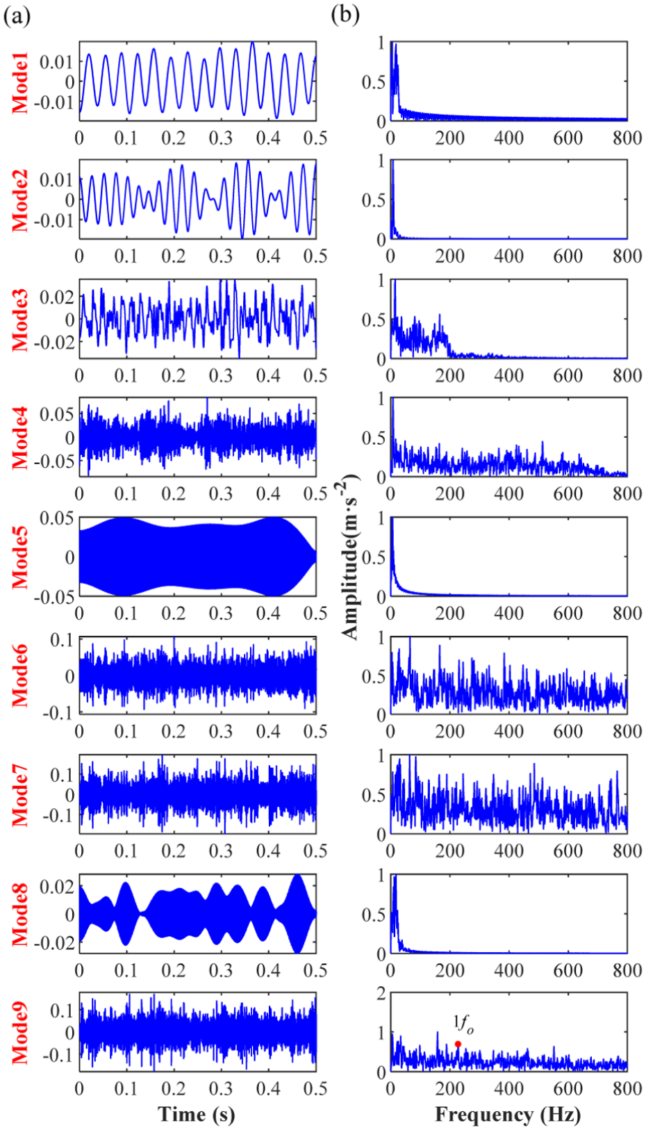
The reconstructed time-domain modal components and normalized envelope spectrum of EFD under case 1: (a) time-domain waveform and (b) normalized envelope spectrum.

Finally, to further evaluate and compare the performance of different methods, the number of decomposition modes for FMD was preset to 9, and the method was applied to extract fault features from the outer race fault signal. Figure 31 illustrates the modal components from modes 1 to 9 reconstructed by FMD, along with their corresponding normalized envelope spectra. As shown in Figure 31(b), the fault characteristic frequency 1f_o can be clearly identified in the normalized envelope spectrum of mode 7. In summary, while the fault information extracted by FMD is more prominent than that in Figures 28 and 30, it remains less effective than the results shown in Figure 26. This comparison further demonstrates the superiority of the proposed AEWFMD method over EWT, EFD, and FMD. Furthermore, unlike the proposed method, EWT, EFD, and FMD lack adaptivity in determining the optimal number of decomposition modes.

Figure 31.

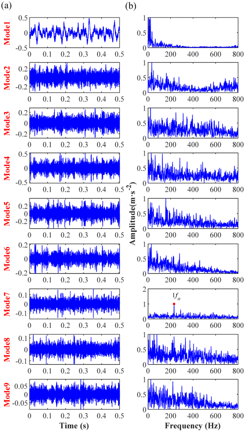
The reconstructed time-domain modal components and normalized envelope spectrum of FMD under case 1: (a) time-domain waveform and (b) normalized envelope spectrum.

Case 2: Application in fault diagnosis of rolling elements in high-speed train axlebox bearings

To verify the effectiveness of the proposed method in diagnosing faults within railway passenger car axlebox bearings, data collected from the wheelset bearing test rig⁵³ (as shown in Figure 32) were utilized for analysis. The test rig primarily consists of five functional modules: the foundational frame, drive unit, loading mechanism, wheelset bearings, and the control system. During the experiment, the shaft speed was maintained at approximately 846 rpm (f_r = 14.1 Hz). Detailed geometric parameters of the tested bearing are provided in Table 2. The defects on the rolling element and the outer race were implanted artificially with a width of 0.2 mm and a depth of 0.3 mm. The sampling frequency was configured at 12.8 kHz with a signal length of 8192 points. Based on the bearing geometry and kinematic relations, the theoretical fault characteristic frequency of the rolling element (f_b) was calculated to be approximately 48.4 Hz.

Figure 32.

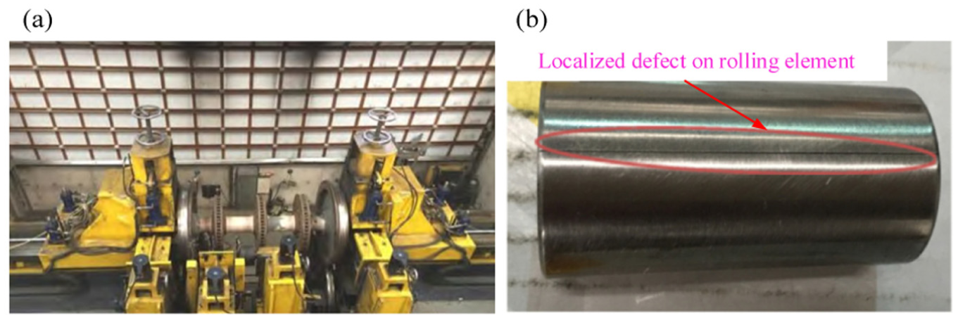
High-speed train axle box test platform and its rolling element faulty bearing: (a) high-speed train axle box test platform and (b) rolling element faulty bearing.⁵³

Table 2.

The geometric parameters of the rolling element faulty bearing in case 2.

Pitch diameter (mm)	Ball diameter (mm)	Number of rollers	Contact angle
187.21	26.69	17	12.8°

Figure 33(a) and (b) presents the time-domain waveform and the corresponding envelope spectrum of the selected raw vibration signal, respectively. As observed in the time-domain waveform (Figure 33(a)), the periodic impulses are obscured by significant background noise and anomalous high-amplitude pulses. Consequently, in the envelope spectrum shown in Figure 33(b), the fault characteristic frequency of the rolling element (1f_b) is hardly discernible due to the heavy noise interference. This reflects a weak fault condition of the bearing, where conventional diagnostic methods fail to identify the fault type, thereby highlighting the challenge of extracting features from such low SNR data.

Figure 33.

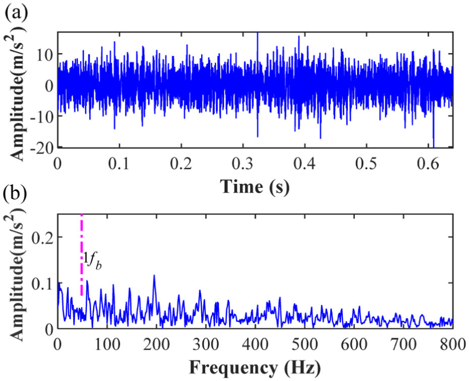
Time waveform and envelope spectrum of rolling element fault signal under case 2: (a) time waveform and (b) envelope spectrum.

First, the proposed AEWFMD method is applied to extract fault features from the rolling element signal. The ST spectrum, illustrated in Figure 34, is calculated, and the mean energy is derived to construct the spectral trend line. Subsequently, the reference frequency is set as f_m = f_b = 48.4 Hz. Within the candidate set [0.5f_m, 1f_m, 1.5f_m, 2f_m, 2.5f_m, 3f_m], the OSF with various window widths W_OSF is utilized to perform moving average filtering on the spectral energy lines, yielding a series of smoothed candidate curves. Then, the maximum ORCER values for the modal components under different spectral lines are recorded. It is found that the ORCER reaches its maximum of 32.1600 when W_OSF is 1.5f_m. The corresponding optimal spectral line, shown as the purple curve in Figure 35, aligns consistently with the overall spectral trend. Finally, all local minima of the optimal spectral line are identified as segmentation boundaries (indicated by red dashed lines in Figure 35) to adaptively partition the spectrum. An empirical wavelet filter bank, adaptively constructed based on these boundaries, is then employed to filter each sub-band, resulting in ten reconstructed modal components (modes 1–10), as shown in Figure 36. This demonstrates that the AEWFMD method eliminates the need for presetting the number of decomposition modes and enables autonomous, rational spectral partitioning and modal reconstruction.

Figure 34.

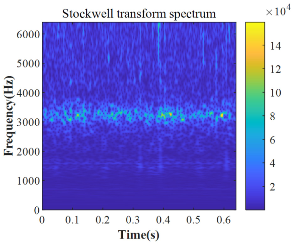
ST spectrum under case 2. ST: Stockwell Transform.

Figure 35.

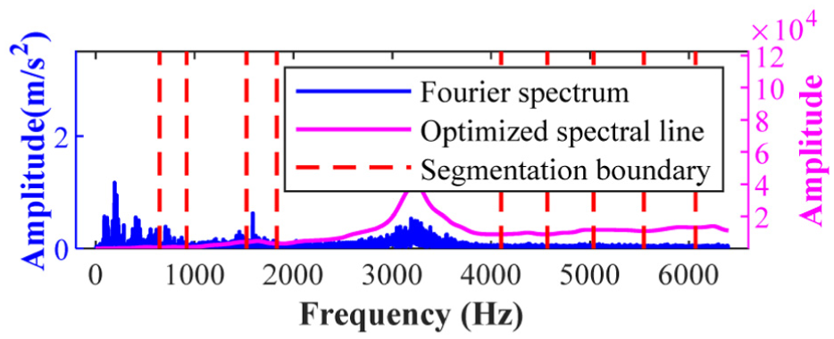
Optimal spectral line and segmentation boundaries of AEWFMD under case 2. AEWFMD: adaptive empirical wavelet filter banks.

Figure 36.

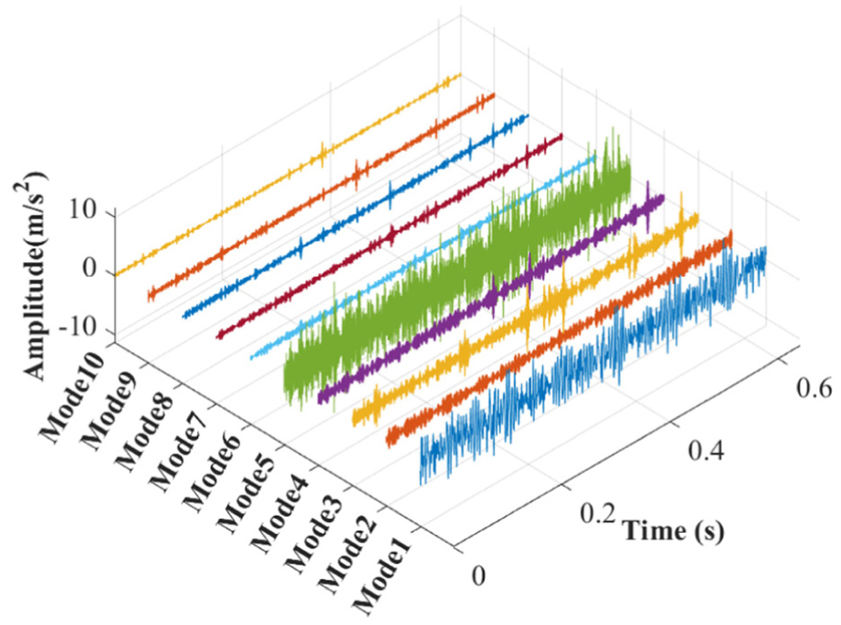
The reconstructed time-domain modal components of AEWFMD under case 2. AEWFMD: adaptive empirical wavelet filter banks.

Subsequently, the OFCER index is utilized to quantitatively evaluate modes 1 through 10, with the results presented in Figure 37. As observed, the maximum OFCER value corresponds to mode 9, identifying it as the optimal modal component for fault identification. Finally, Figure 38(a) and (b) illustrates the time-domain waveform and the normalized envelope spectrum of mode 9, respectively. In Figure 38(b), the extracted fault characteristic frequencies (1f_b to 5f_b) are clearly identifiable. Consequently, the rolling element fault in the bearing is accurately diagnosed with high reliability, validating the effectiveness and practicality of the proposed AEWFMD method.

Figure 37.

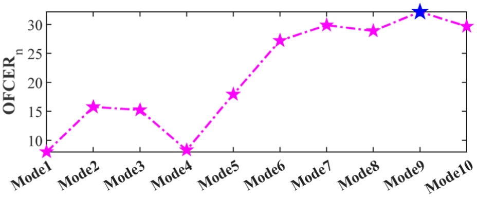
OFCER indicator values for each reconstructed time-domain modal component under case 2. OFCER: optimized fault characteristic energy ratio.

Figure 38.

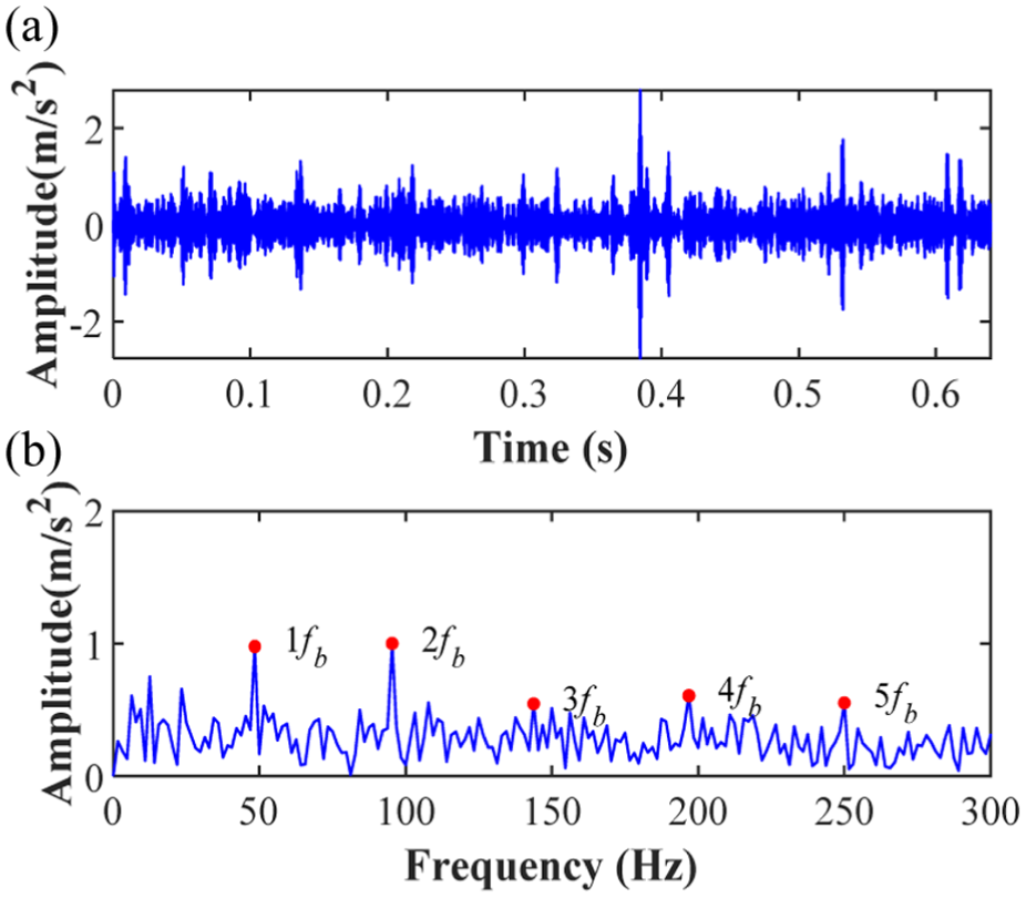
The time-domain waveform of mode 9 and its normalized envelope spectrum under case 2: (a) time-domain waveform and (b) normalized envelope spectrum.

Secondly, to evaluate the comparative performance, the EWT method is implemented with the number of decomposition modes preset to 10 to extract features from the rolling element fault signal. Figure 39 illustrates the spectral segmentation boundaries generated by the EWT method. As shown in Figure 39(a), a high density of segmentation boundaries is observed within the 0–300 Hz range. Specifically, the enlarged view in Figure 39(b) reveals three closely spaced boundaries near 200 Hz. Such redundant partitioning leads to spectral over-decomposition, which potentially triggers the generation of irrelevant or spurious components. Subsequently, the reconstructed modal components (modes 1–10) and their corresponding normalized envelope spectra are presented in Figure 40. Finally, it is observed from Figure 40(b) that only a faint trace of the fault characteristic frequency 1f_b is identifiable in the envelope spectrum of mode 8, making it difficult to accurately determine the bearing fault type. These results indicate that the EWT method suffers from excessively dense spectral partitioning and the inherent requirement for a predefined number of modes, both of which hinder accurate fault diagnosis.

Figure 39.

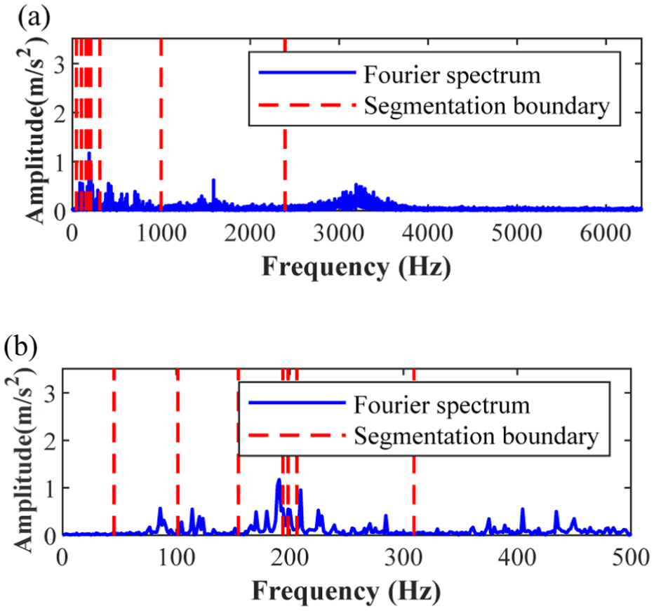
Spectrum segmentation boundaries of EWT under case 2: (a) segmentation boundaries and (b) enlarged view of the spectrum segmentation boundaries. EWT: empirical wavelet transform.

Figure 40.

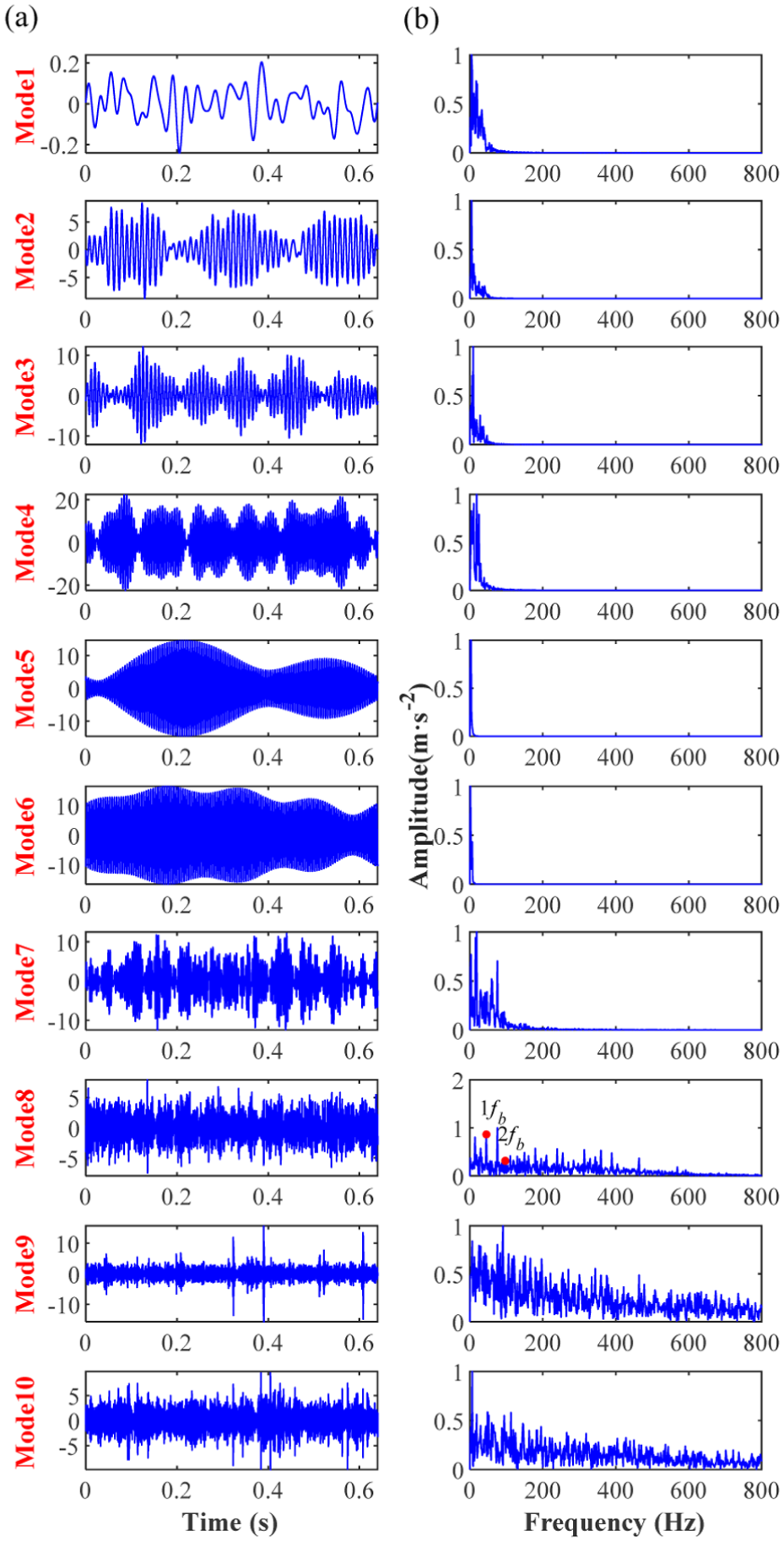
The reconstructed time-domain modal components and normalized envelope spectrum of EWT under case 2: (a) time-domain waveform and (b) normalized envelope spectrum. EWT: empirical wavelet transform.

Then, for further comparative analysis, the number of decomposition modes for the EFD method is also preset to 10. As observed in Figure 41(a), the boundaries are again densely distributed within the 0–300 Hz range. Specifically, the enlarged view in Figure 41(b) reveals four closely spaced boundaries near 200 Hz. Compared with Figure 35, both EFD and EWT suffer from excessively dense spectral partitioning. Figure 42 illustrates the modal components and their corresponding normalized envelope spectra. Finally, it is observed from Figure 42(b) that only a faint fault characteristic frequency 1f_b is discernible in the normalized envelope spectrum of mode 8, making it difficult to accurately identify the bearing fault type.

Figure 41.

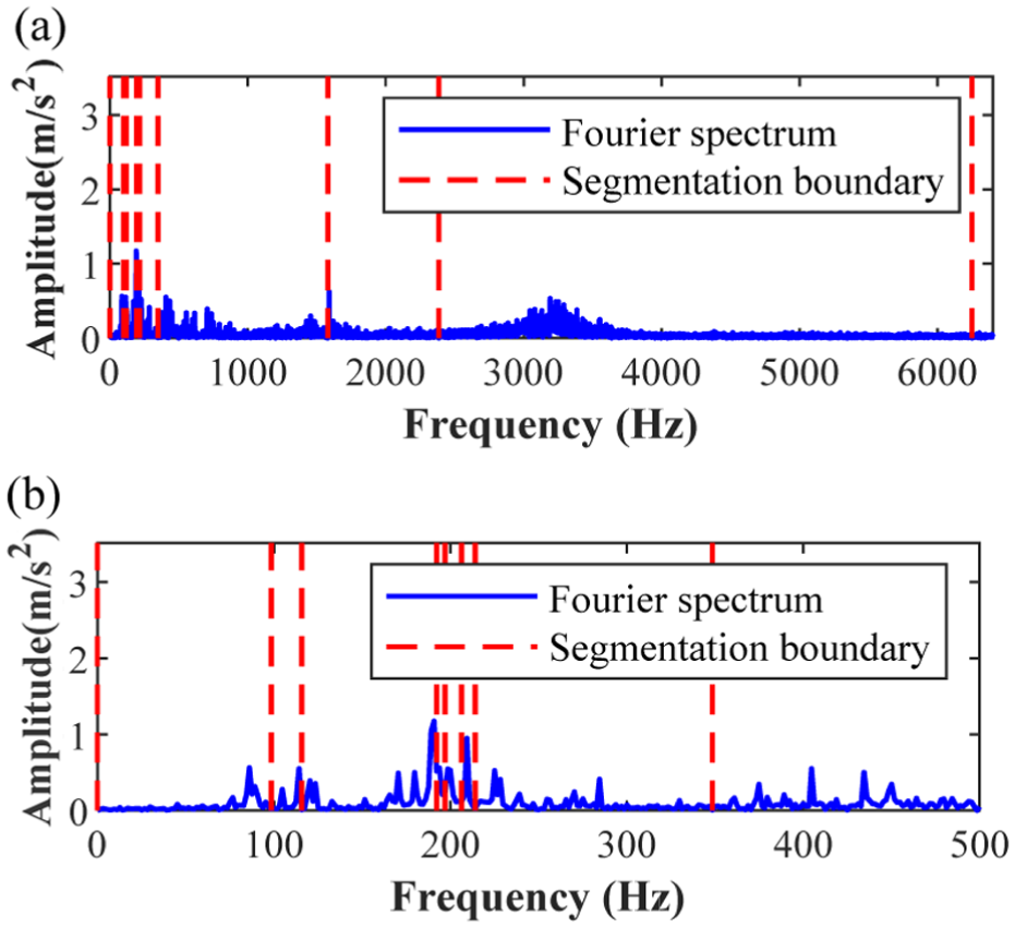
Spectrum segmentation boundaries of EFD under case 2: (a) segmentation boundaries and (b) enlarged view of the spectrum segmentation boundaries.

Figure 42.

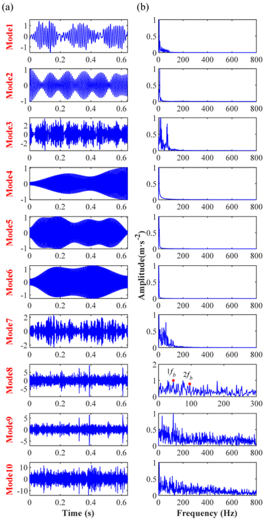
The reconstructed time-domain modal components and normalized envelope spectrum of EFD under case 2: (a) time-domain waveform and (b) normalized envelope spectrum.

Finally, the decomposition mode count for FMD is preset to 10. Figure 43 illustrates the reconstructed modal components and their normalized envelope spectra. As shown in Figure 43(b), although the fault frequencies 1f_b and 2f_b are successfully extracted in mode 10, and the result is more prominent than those in Figures 40 and 42, it remains less effective than the performance shown in Figure 38. In summary, these results demonstrate the superiority of the proposed AEWFMD method over EWT, EFD, and FMD. Furthermore, unlike the proposed method, EWT, EFD, and FMD lack the adaptivity required to determine the optimal number of decomposition modes, which limits their applicability in complex diagnostic scenarios.

Figure 43.

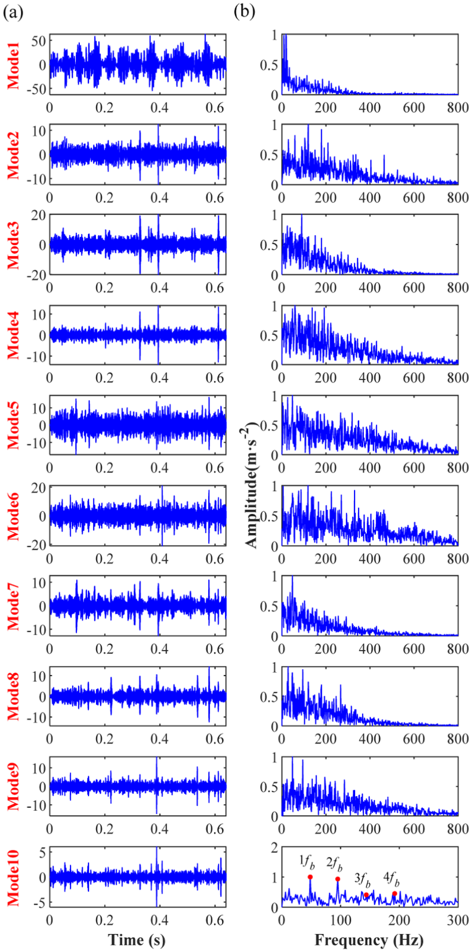
The reconstructed time-domain modal components and normalized envelope spectrum of FMD under case 2: (a) time-domain waveform and (b) normalized envelope spectrum.

Case 3: Application in the diagnosis of artificial compound fault bearings

To further evaluate the applicability of the proposed method in diagnosing compound faults involving the bearing outer race and rolling elements, the dataset provided by the HUST⁵⁴ is utilized for validation. The basic architecture of the test rig is illustrated in Figure 44. The test bench consists of a 750 W (1 HP) induction motor driving a multi-step shaft and a powder brake of Leroy Somer. A PCB 352C33 accelerometer is mounted in the vertical direction of the tested bearing to acquire vibration data. To simulate the initial state of the bearing failure, micro-crack defects with a width of 0.2 mm are created on the outer race and rolling elements using wire-cut electrical discharge machining. Detailed geometric parameters of the tested KG6206 bearing are listed in Table 3. During signal acquisition, the shaft speed is maintained at 1490 rpm (corresponding to a rotating frequency f_r = 24.83 Hz). The sampling frequency is set to 51.2 kHz with a total of 512,000 sampling points. Based on these parameters, the calculated fault characteristic frequencies for the outer race (f_o) and the rolling element f_b) are 89.9 and 122 Hz. Note that the calculated f_b here is approximately twice the actual calculated f_b.

Figure 44.

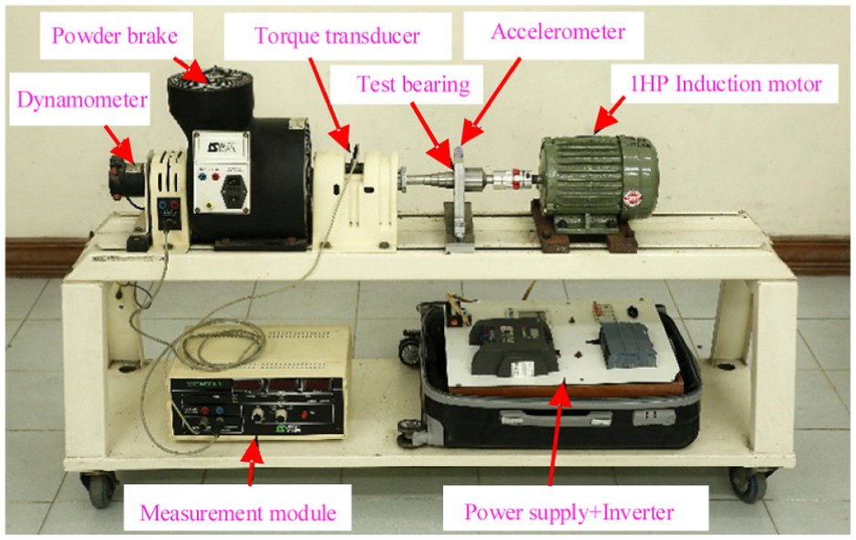
Bearing fault simulation test bench.⁵⁴

Table 3.

The geometric parameters of the composite faulty bearing in case 3.

Pitch diameter (mm)	Ball diameter (mm)	Number of rollers	Contact angle
46	9	9	0°

Figure 45 illustrates the time-domain waveform and the corresponding envelope spectrum of the selected raw vibration signal. As observed in the time-domain waveform (Figure 45(a)), the signal is corrupted by interference components such as background noise. Furthermore, the periodic fault impulses from the rolling elements and the outer race are coupled with each other, making the individual impulse features indistinct. In the envelope spectrum shown in Figure 45(b), it is difficult to distinguish the characteristic frequencies of both the rolling element and the outer race due to this mutual coupling and noise masking. Consequently, the specific fault types of the bearing cannot be fully determined through conventional analysis, highlighting the inherent complexity of diagnosing weak compound faults.

Figure 45.

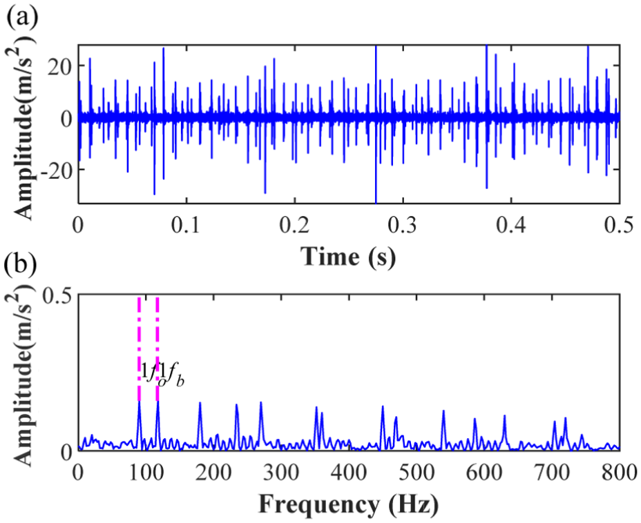
Time waveform and envelope spectrum of rolling element and outer ring fault signal: (a) time waveform and (b) envelope spectrum.

First, the proposed AEWFMD method is employed to separate and extract rolling element fault features from the compound fault signal. Initially, the ST spectrum is calculated, as illustrated in Figure 46. Significant energy concentrations are observed within the 3000–12,000 Hz and around 20,000 Hz, which align precisely with the resonance bands of the outer race and rolling elements in the compound fault. Based on this, the mean energy is derived to construct the spectral trend line. Subsequently, with the reference frequency set to f_m = f_b = 122 Hz, the OSF with various window widths W_OSF within the candidate set [0.5f_m, 1f_m, 1.5f_m, 2f_m, 2.5f_m, 3f_m] is utilized to perform moving average filtering on the spectral energy lines, yielding a series of candidate curves. Next, the maximum ORCER values for the modal components under different spectral lines are calculated and recorded. It is found that the ORCER reaches its maximum of 32.4162 when the window width W_OSF is 2.5f_m. The corresponding optimal spectral line, represented by the purple curve in Figure 47, exhibits high consistency with the overall spectral trend. Subsequently, all local minima of the optimal spectral line are identified to define the segmentation boundaries (indicated by the red dashed lines in Figure 47), allowing for the adaptive division of the spectrum into multiple frequency bands. Following this, an empirical wavelet filter bank is adaptively constructed based on these boundaries to filter each sub-band, resulting in nine reconstructed modal components (modes 1–9), as shown in Figure 48. This demonstrates that the proposed AEWFMD method effectively achieves autonomous spectral partitioning and modal reconstruction without the need for a predefined number of modes.

Figure 46.

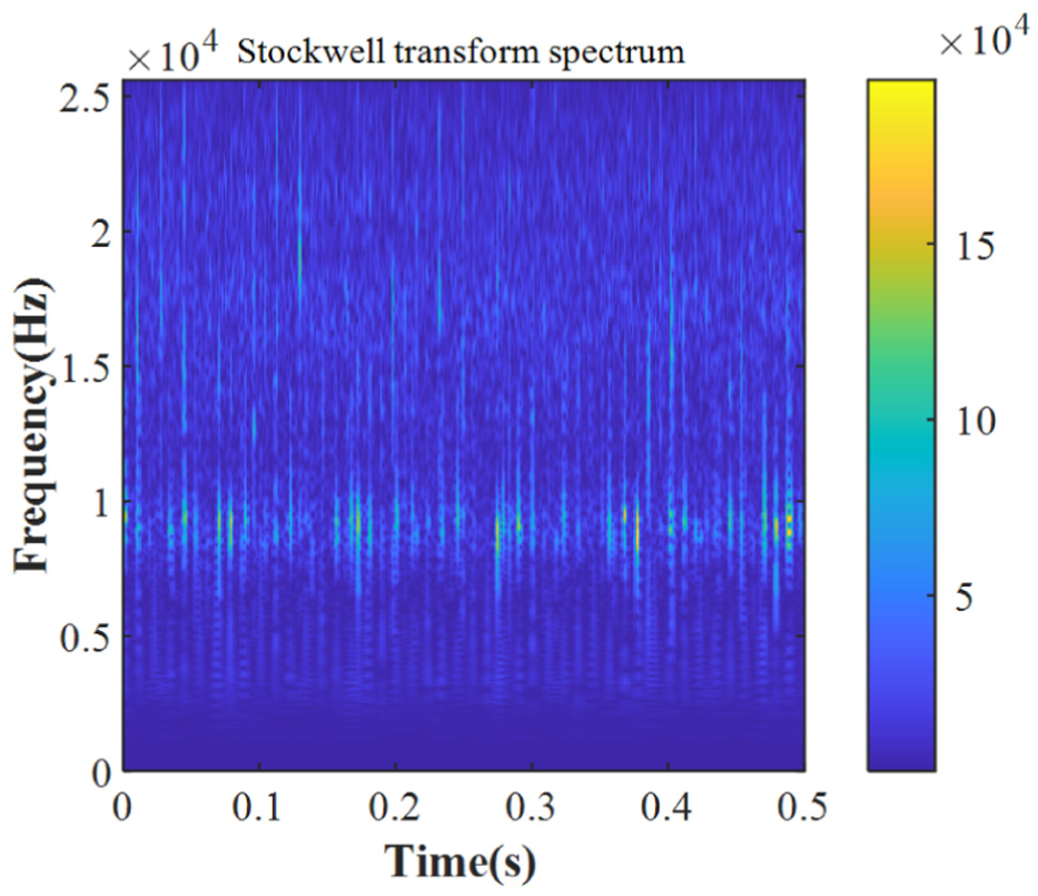
ST spectrum under case 3. ST: Stockwell Transform.

Figure 47.

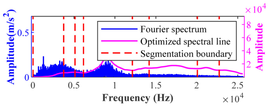
Optimal spectral line and segmentation boundaries of AEWFMD under rolling element fault in case 3. AEWFMD: adaptive empirical wavelet filter banks.

Figure 48.

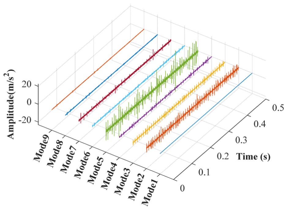
The reconstructed time-domain modal components of AEWFMD under rolling element fault in case 3. AEWFMD: adaptive empirical wavelet filter banks.

Subsequently, the OFCER index is employed to quantitatively evaluate modes 1 through 9, with the results presented in Figure 49. As illustrated, the maximum OFCER value is represented by the blue region, which corresponds to mode 7. Consequently, mode 7 is identified as the optimal modal component. Furthermore, the frequency band division of mode 7 aligns precisely near the right side of 20,000 Hz, demonstrating the rationality of the boundary division determined by the proposed optimal spectral line. Finally, the time-domain waveform and normalized envelope spectrum of mode 7 are provided in Figure 50(a) and (b), respectively. In Figure 50(b), the rolling element fault characteristic frequencies (1f_b to 6f_b) are clearly observable. These findings facilitate an accurate diagnosis of the rolling element fault in the bearing, thereby validating the high reliability of the diagnostic approach.

Figure 49.

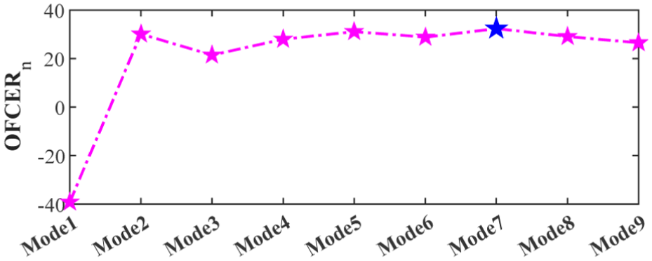
OFCER indicator values for each reconstructed time-domain modal component under rolling element fault in case 3. OFCER: optimized fault characteristic energy ratio.

Figure 50.

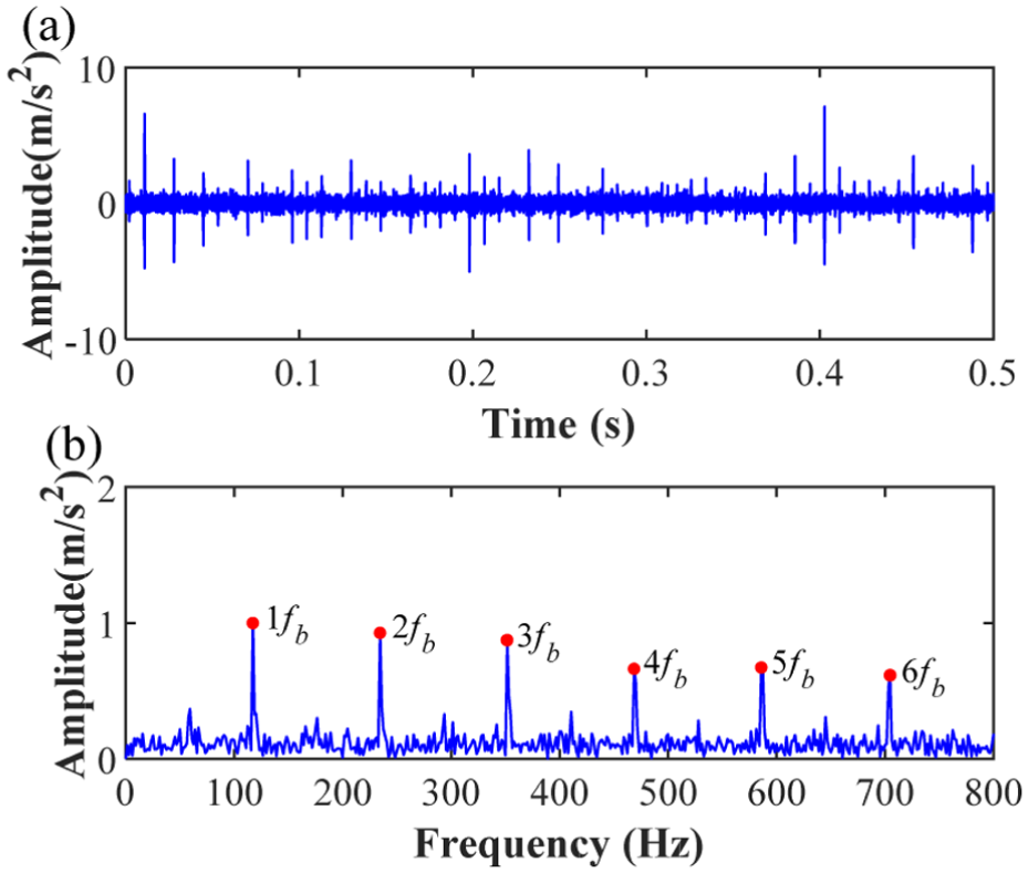
The time-domain waveform of mode 7 and its normalized envelope spectrum under rolling element fault in case 3: (a) time-domain waveform; and (b) normalized envelope spectrum.

Subsequently, the proposed AEWFMD method is employed to extract outer race fault features from the compound fault signal. Initially, the ST spectrum, as illustrated in Figure 46, is computed, and its energy mean is utilized to construct the spectral trend line. With the reference frequency set to f_m = f_o = 89.9 Hz, various window widths W_OSF within the set [0.5f_m, 1f_m, 1.5f_m, 2f_m, 2.5f_m, 3f_m] are selected to perform moving average filtering on the spectral energy lines via OSF, yielding a series of candidate spectral lines. Next, the maximum ORCER values of the modal components under different spectral lines are calculated and recorded. It is found that the ORCER value reaches its maximum of 36.6043 when the window width W_OSF. The corresponding optimal spectral line, represented by the purple curve in Figure 51, exhibits high consistency with the spectral trend. Subsequently, all local minima of the optimal spectral line are identified to define the segmentation boundaries (indicated by the red dashed lines in Figure 51), allowing for the adaptive division of the spectrum into multiple frequency bands.

Figure 51.

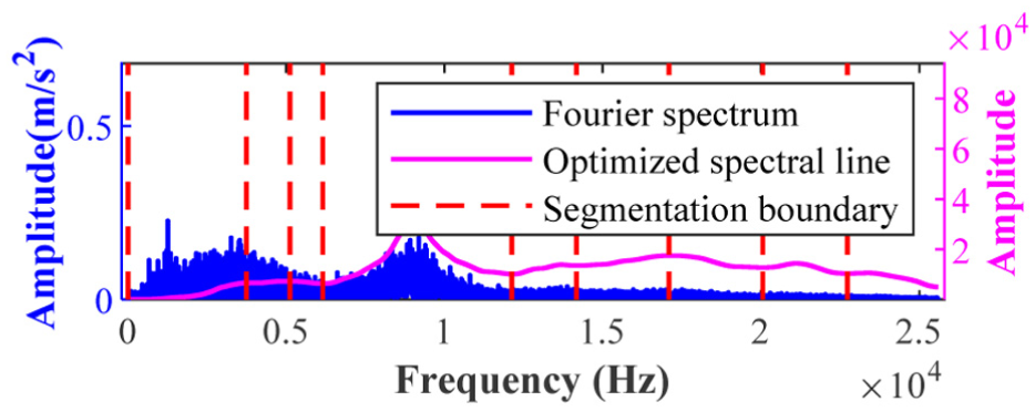
Optimal spectral line and segmentation boundaries of AEWFMD under outer ring fault in case 3. AEWFMD: adaptive empirical wavelet filter banks.

Following this, an empirical wavelet filter bank is adaptively constructed based on these boundaries to filter each sub-band, resulting in ten reconstructed modal components (modes 1–10), as shown in Figure 52. These results demonstrate that the proposed AEWFMD method effectively achieves autonomous spectral partitioning and modal reconstruction without the need for a predefined number of modes.

Figure 52.

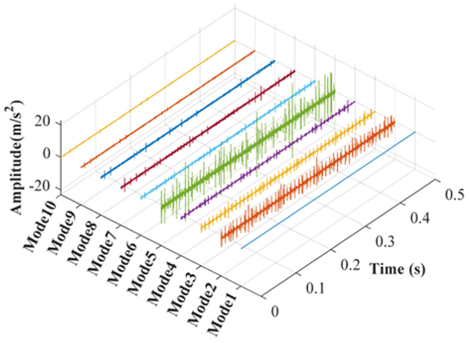
The reconstructed time-domain modal components of AEWFMD under outer ring fault in case 3. AEWFMD: adaptive empirical wavelet filter banks.

Then, the OFCER index is utilized to quantitatively evaluate modes 1 through 10, as illustrated in Figure 53. It can be observed that the maximum OFCER value, indicated by the blue region, corresponds to mode 3. Therefore, mode 3 is identified as the optimal modal component. As shown in Figure 46, the frequency band division of mode 3 aligns precisely within the 3000–12,000 Hz range, which validates the rationality of the boundary division determined by the proposed optimal spectral line.

Figure 53.

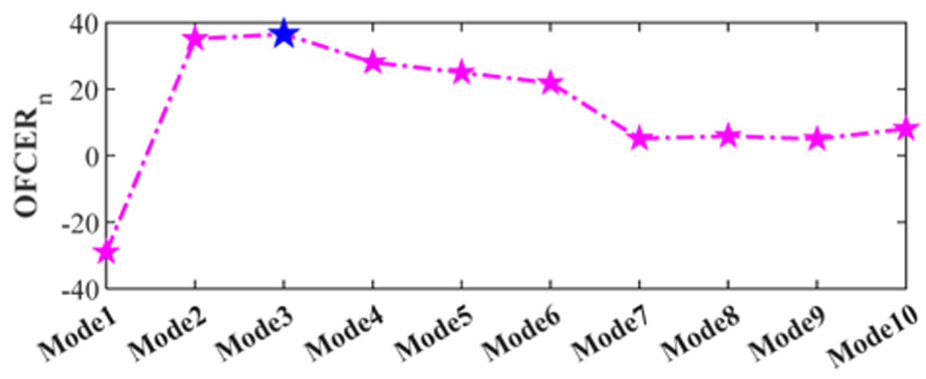
OFCER indicator values for each reconstructed time-domain modal component under outer ring fault in case 3. OFCER: optimized fault characteristic energy ratio.

Finally, the time-domain waveform and normalized envelope spectrum of mode 3 are provided in Figure 54(a) and (b), respectively. In Figure 54(b), the extracted outer race fault characteristic frequencies and their harmonics (1f_o to 8f_o) are clearly discernible. Accordingly, the outer race fault of the bearing is accurately diagnosed with high reliability. Integrating the fault feature extraction results from Figures 50 and 54, the proposed AEWFMD method successfully achieves feature separation and extraction for compound faults involving both rolling elements and outer races. This demonstrates the effectiveness and practicality of the AEWFMD method in the diagnosis of complex bearing faults.

Figure 54.

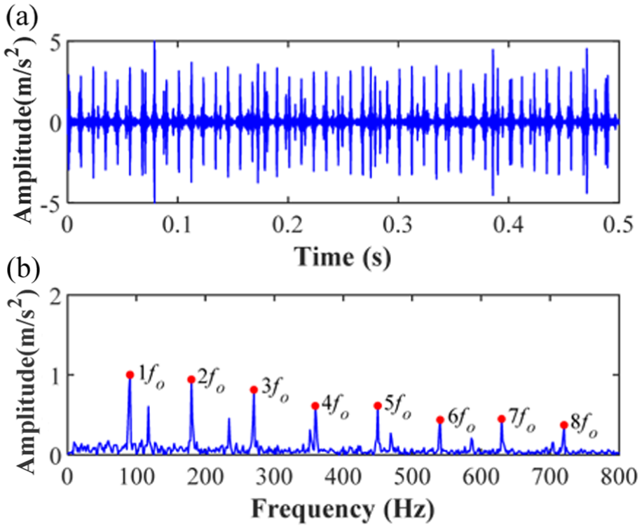
The time-domain waveform of mode 3 and its normalized envelope spectrum under outer ring fault in case 3: (a) time-domain waveform and (b) normalized envelope spectrum.

Next, to perform a comparative analysis, the number of modes for the EWT method is preset to 10 for extracting features from the compound fault signal. Figure 55 illustrates the spectral segmentation boundaries determined by the EWT method. As observed in Figure 55(a), the segmentation boundaries are densely distributed within the 0–10,000 Hz range. Specifically, the enlarged view in Figure 55(b) reveals four closely spaced boundaries near the frequency of 8870 Hz. This clustering leads to over-decomposition of the spectrum, which potentially generates redundant or irrelevant components. Subsequently, the reconstructed modes 1 through 10 and their corresponding normalized envelope spectra are presented in Figure 56. According to Figure 56(b), although the rolling element fault characteristic frequencies (1f_b to 6f_b) are identified in mode 6 and the outer race fault characteristic frequencies (1f_o to 6f_o) are found in mode 2, there is significant interference from high-amplitude spectral lines around the 1f_o to 2f_o range. Consequently, the EWT method yields suboptimal performance in terms of feature separation for compound faults.

Figure 55.

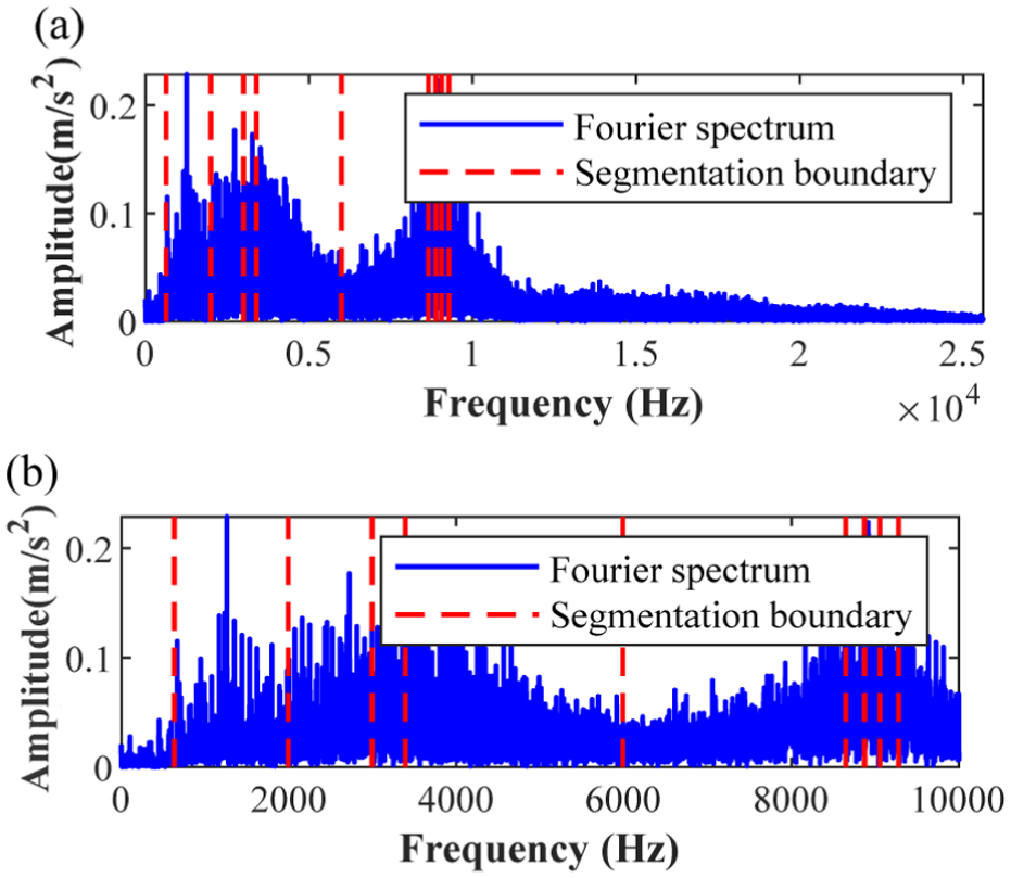
Spectrum segmentation boundaries of EWT under case 3: (a) segmentation boundaries and (b) enlarged view of the spectrum segmentation boundaries. EWT: empirical wavelet transform.

Figure 56.

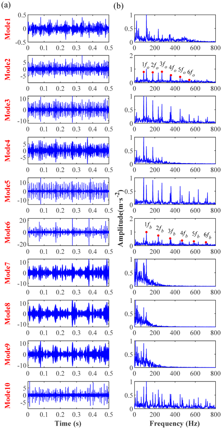
The reconstructed time-domain modal components and normalized envelope spectrum of EWT under case 3: (a) time-domain waveform and (b) normalized envelope spectrum. EWT: empirical wavelet transform.

Next, to conduct a comparative analysis, the number of modes for the EFD method is preset to 10 for feature extraction from the compound fault signal. Figure 57 illustrates the spectral segmentation boundaries determined by the EFD method. As shown in Figure 57(a), the segmentation boundaries are densely distributed within the 0–10,000 Hz frequency range. Specifically, the enlarged view in Figure 57(b) reveals four closely spaced boundaries near 9000 Hz. This clustering leads to over-decomposition of the spectrum, which potentially generates redundant or irrelevant components. Compared with the results in Figure 51, both EFD and EWT exhibit the issue of excessively dense segmentation boundaries. Subsequently, the reconstructed modes 1 through 10 and their corresponding normalized envelope spectra are presented in Figure 58. According to Figure 58(b), although the rolling element fault characteristic frequencies (1f_b to 6f_b) are identified in mode 6 and the outer race fault characteristic frequencies (1f_o to 6f_o) are found in mode 2, there is significant interference from high-amplitude spectral lines around the 1f_o to2f_o range. Consequently, the EFD method yields suboptimal performance in terms of feature separation for compound faults.

Figure 57.

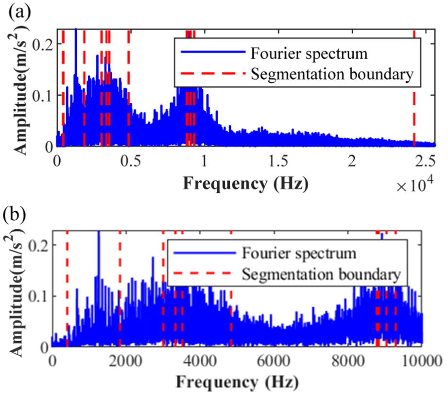
Spectrum segmentation boundaries of EFD under case 3: (a) segmentation boundaries and (b) enlarged view of the spectrum segmentation boundaries.

Figure 58.

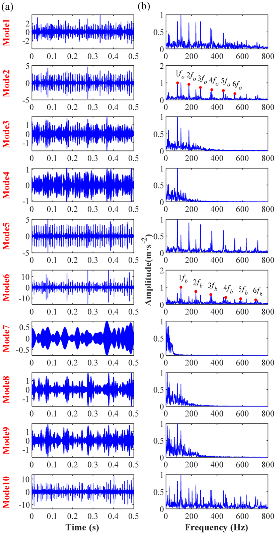
The reconstructed time-domain modal components and normalized envelope spectrum of EFD under case 3: (a) time-domain waveform and (b) normalized envelope spectrum.

Finally, to further evaluate the comparative performance, the number of modes for the FMD method is also preset to 10 for feature extraction from the compound fault signal. Figure 59 presents the reconstructed modes 1 through 10 and their corresponding normalized envelope spectra. As illustrated in Figure 59(b), the rolling element fault characteristic frequencies (1f_b to 6f_b) are identified in mode 8, and the outer race fault frequencies (1f_o to 6f_o) are extracted in mode 2. However, significant interference from high-amplitude spectral lines persists around the 1f_o to 2f_o range, resulting in suboptimal separation performance.

Figure 59.

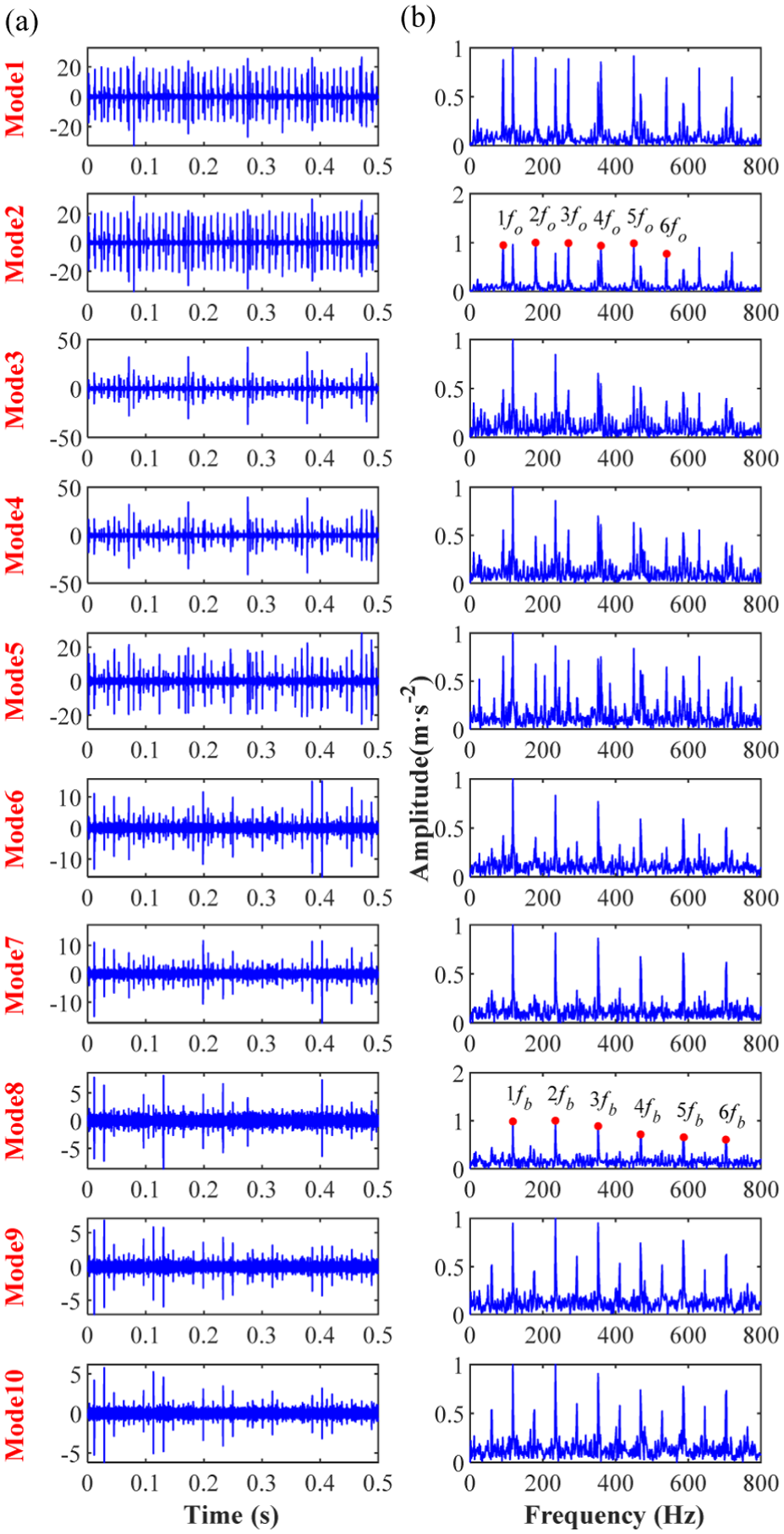
The reconstructed time-domain modal components and normalized envelope spectrum of FMD under case 3:(a) time-domain waveform and (b) normalized envelope spectrum.

Conclusion

To address the inherent limitations of the traditional EWT—specifically its fragile spectral segmentation under intense noise, the lack of parameter adaptivity, and the difficulty in selecting sensitive components—this paper proposes a modal decomposition method for constructing AEWFMD. The proposed method is successfully applied to the diagnosis of both single and compound bearing faults. The primary research findings are summarized as follows:

Construction of a robust spectral trend line based on ST-spectrum energy distribution. By leveraging the multi-resolution characteristics of the ST, high-dimensional time-frequency features are mapped into a macroscopic physical trend line through frequency-slice energy averaging. This mechanism effectively suppresses random noise and transient impulsive interference from an energy evolution perspective. It establishes a robust physical foundation for subsequent adaptive boundary partitioning, overcoming the sensitivity of traditional spectra to background noise.

Development of a parameter adaptive optimization strategy driven by the OFCER index. This paper proposes the OFCER as the objective function to achieve dynamic optimization of the optimal window width (W_OSF) for the OSF. The results demonstrate that the selected window range [0.5f_m, 3f_m] maintains universality across varying noise levels and fault characteristic frequencies f_m. This significantly enhances the algorithm’s adaptive adjustment capability and facilitates the autonomous determination of the number of decomposition modes.

Establishment of a precise fault feature identification framework via AEWFMDA bidirectional optimization logic centered on the OFCER index was established. The “front-end” directs the adaptive reconstruction of the filter bank, while the “back-end” enables the automated selection of sensitive modes. Simulation results confirm that even under extreme noise conditions (SNR = −15 dB), the method accurately identifies resonance band boundaries and locks onto optimal modal components. The segmentation boundaries exhibit excellent convergence, approaching the resonance frequencies from both directions.

Validation of superiority in compound fault diagnosis. Comparative analysis indicates that AEWFMD significantly outperforms EWT, EFD, and FMD in extracting fault signatures. Particularly when processing compound signals containing both inner and outer race faults, AEWFMD effectively decouples and identifies distinct resonance bands, providing a robust methodological framework for the health monitoring of rotating machinery.

Limitations and future work. Currently, the proposed method maintains a degree of dependence on prior knowledge of fault characteristic frequencies. Future research will explore adaptive mechanisms based on signal periodicity to eliminate this dependency. Furthermore, subsequent efforts will focus on the organic integration of the AEWFMD method with deep learning algorithms, utilizing the physical interpretability of traditional signal processing to guide the neural network’s learning process, thereby achieving more efficient and intelligent fault diagnosis.

Footnotes

Acknowledgements

The authors would like to appreciate the anonymous reviewers and the editor for their helpful comments. Meanwhile, the authors would like to appreciate IMS, Southwest Jiaotong University and HUST for providing free downloadable fault bearing data.

ORCID iD

Rui Guo

Ce Gao

Funding

The authors disclosed receipt of the following financial support for the research, authorship, and/or publication of this article: This work is supported by the National Natural Science Foundation of China (numbers 12173054 and 52405073), Outsourced Projects of Sichuan Gas Turbine Establishment, Aero Engine Corporation of China (GJCZ-0201-02 and GJCZ-0303-03), and the Tianjin Science and Technology Plan Project (25YDTPJC00190), which is highly appreciated by the authors.

Declaration of conflicting interests

The authors declared no potential conflicts of interest with respect to the research, authorship, and/or publication of this article.

References

Zhou

Xing

Zou

, et al. EMGGDFuRDE: enhancive multiscale generalized Gaussian distribution fuzzy Renyi dispersion entropy and its application in wind turbines fault diagnosis. Mech Syst Signal Process 2025; 231:112636. https://doi.org/10.1016/j.ymssp.2025.112636

Song

Jin

Lin

, et al. Remaining useful life prediction method based on the spatiotemporal graph and GCN nested parallel route model. IEEE Trans Instrum Meas 2024; 73: 1–12. https://doi.org/10.1109/TIM.2024.3370801

Liu

, et al. A hybrid method combining Lévy process and neural network for predicting remaining useful life of rotating machinery. Adv Eng Inform 2024; 61: 102490. https://doi.org/10.1016/j.aei.2024.102490

Fan

Peng

Shen

, et al. Variable scale multilayer perceptron for helicopter transmission system vibration data abnormity beyond efficient recovery. Eng Appl Artif Intell 2024; 133: 108184. https://doi.org/10.1016/j.engappai.2024.108184

Cao

Meng

, et al. A bearing fault diagnosis method for unknown operating conditions based on differentiated feature extraction. ISA Trans 2025; 156: 468–478. https://doi.org/10.1016/j.isatra.2024.10.024

Peng

Shen

, et al. Rolling bearing fault diagnosis under data imbalance and variable speed based on adaptive clustering weighted oversampling. Reliab Eng Syst Saf 2024; 244: 109938. https://doi.org/10.1016/j.ress.2024.109938

Wang

Jiang

Zhu

, et al. A deep feature enhanced reinforcement learning method for rolling bearing fault diagnosis. Adv Eng Inform 2022; 54: 101750. https://doi.org/10.1016/j.aei.2022.101750

Meng

Wang

Liu

, et al. Velocity-matching extraction demodulation transform for nonstationary signal analysis of rolling bearings. IEEE Trans Instrum Meas 2025; 74: 1–11. https://doi.org/10.1109/TIM.2024.3509535

Sun

Meng

Liu

, et al. A novel compound fault diagnosis for rolling bearing based on sparse harmonic feature mode decomposition and enhanced spectral amplitude modulation. Mech Syst Signal Process 2025; 239: 113343. https://doi.org/10.1016/j.ymssp.2025.113343

10.

Qin

Zhao

Chen

, et al. Learnable wavelet-driven physically interpretable networks for bearing fault diagnosis under variable speed. Mech Syst Signal Process 2025; 237: 113121. https://doi.org/10.1016/j.ymssp.2025.113121

11.

Fang

Chang

, et al. A digital twin-enabled domain adaptation network for cross-space fault diagnosis of roller bearings. Mech Syst Signal Process 2025; 236: 113053. https://doi.org/10.1016/j.ymssp.2025.113053

12.

Mahela

Khan

Alhelou

, et al. Power quality assessment and event detection in distribution network with wind energy penetration using Stockwell Transform and fuzzy clustering. IEEE Trans Ind Inf 2020; 16: 6922–6932. https://doi.org/10.1109/TII.2020.2971709

13.

Zhang

Huang

Xia

. An improved multi-taper S-Transform method to estimate evolutionary spectrum and time-varying coherence of nonstationary processes. Mech Syst Sig Process 2023; 198:110386. https://doi.org/10.1016/j.ymssp.2023.110386

14.

Zhang

Yang

Ren

, et al. Time-varying characteristics analysis of vehicle-bridge interaction system based on modified S-transform reassignment technique. Mech Syst Sig Process 2021; 160: 107807. https://doi.org/10.1016/j.ymssp.2021.107807

15.

Ying

Noman

, et al. Stockwell transform spectral amplitude modulation method for rotating machinery fault diagnosis. Mech Syst Signal Process 2025; 223: 111884. https://doi.org/10.1016/j.ymssp.2024.111884

16.

Liu

Xiang

Jiang

, et al. Second-order transient-extracting S transform for fault feature extraction in rolling bearings. Reliab Eng Syst Saf 2023; 230: 108955. https://doi.org/10.1016/j.ress.2022.108955

17.

Xie

Xiao

Huang

, et al. Attention-augmented stockwell transform and convolutional neural network framework for electroencephalogram-based multi-class classification of Frontotemporal Dementia. Inform Fusion 2025; 123: 103267. https://doi.org/10.1016/j.inffus.2025.103267

18.

Xiao

Song

, et al. Diagnosis of distribution network fault using multiresolution S-transform and modified convolution neural network. Int J Electr Power Energy Syst 2024; 162: 110294. https://doi.org/10.1016/j.ijepes.2024.110294

19.

Shi

Zhang

Yang

, et al. A method for food origin identification and ingredient content prediction based on S-transform and multi-task deep learning. J Food Compos Anal 2025; 147: 108123. https://doi.org/10.1016/j.jfca.2025.108123

20.

Luo

Shao

Lin

, et al. Meta-learning with elastic prototypical network for fault transfer diagnosis of bearings under unstable speeds. Reliab Eng Syst Saf 2024; 245: 110001. https://doi.org/10.1016/j.ress.2024.110001

21.

Jiang

Wang

, et al. Multi-sensor data fusion-enabled semi-supervised optimal temperature-guided PCL framework for machinery fault diagnosis. Informat Fusion 2024; 101: 16. https://doi.org/10.1016/j.inffus.2023.102005

22.

Zhao

Cui

Liu

. Bearing weak fault feature extraction under time-varying speed conditions based on frequency matching demodulation transform. IEEE ASME Trans Mechatron 2023; 28(3): 1627–1637. https://doi.org/10.1109/TMECH.2022.3215545

23.

Huang

Shen

Long

, et al. The empirical mode decomposition and the Hilbert spectrum for nonlinear and non-stationary time series analysis. Proc R Soc Lond Ser A 1998; 454. https://doi.org/10.1098/rspa.1998.0193

24.

Huang

. Ensemble empirical mode decomposition: a noise-assisted data analysis method. Adv Data Sci Adapt Anal 2011; 1: 1–41. https://doi.org/10.1142/S1793536909000047

25.

Yeh

Shieh

Huang

. Complementary ensemble empirical mode decomposition: a novel noise enhanced data analysis method. Adv Data Sci Adapt Anal 2010; 2(2): 135–156. https://doi.org/10.1142/S1793536910000422

26.

Torres

Colominas

Schlotthauer

, et al. A complete ensemble empirical mode decomposition with adaptive noise. In: 2011 IEEE international conference on acoustic, speech and signal processing (ICASSP), Prague Congress Center, Prague, Czech Republic, 22–27 May 2011, vol. 2, no. 1, pp. 4144–4147. IEEE.

27.

Ying

Zheng

Pan

, et al. Permutation entropy-based improved uniform phase empirical mode decomposition for mechanical fault diagnosis. Digital Signal Process 2021; 117: 103167. https://doi.org/10.1016/j.dsp.2021.103167

28.

Dragomiretskiy

Zosso

. Variational mode decomposition. IEEE Trans Signal Process 2013; 62(3): 531–544. https://doi.org/10.1109/TSP.2013.2288675

29.

Nazari

Sakhaei

. Variational mode extraction: a new efficient method to derive respiratory signals from ECG. IEEE J Biomed Health Inf 2018; 22(4): 1059–1067. https://doi.org/10.1109/JBHI.2017.2734074

30.

Pan

Yang

, et al. Symplectic geometry mode decomposition and its application to rotating machinery compound fault diagnosis. Mech Syst Signal Process 2019; 114: 189–211. https://doi.org/10.1016/j.ymssp.2018.05.019

31.

Pan

Zhang

Cheng

, et al. Symplectic geometry transformation-based periodic segment method: algorithm and applications. IEEE Trans Instrum Meas 2023; 72: 1–8. https://doi.org/10.1109/TIM.2023.3271006

32.

Cheng

Yang

, et al. Symplectic Ramanujan mode decomposition and its application to compound fault diagnosis of bearings. ISA Trans 2022; 129:495–503. https://doi.org/10.1016/j.isatra.2021.12.013

33.

Guo

Xiang

. Cycle kurtosis entropy guided symplectic geometry mode decomposition for detecting faults in rotating machinery. ISA Trans 2023; 138: 546–561. https://doi.org/10.1016/j.isatra.2023.03.026

34.

Yan

Hou

, et al. Compound fault diagnosis method for rolling bearings based on enhanced MED and adaptive periodized symplectic geometry mode decomposition. Struct Health Monit 2025: 1: 31. https://doi.org/10.1177/14759217251314703

35.

Gilles

. Empirical wavelet transform. IEEE Trans Signal Process 2013; 61(16): 3999–4010. https://doi.org/10.1109/TSP.2013.2265222

36.

Wang

Zhao

, et al. Sparsity guided empirical wavelet transform for fault diagnosis of rolling element bearings. Mech Syst Signal Process 2018; 101: 292–308. https://doi.org/10.1016/j.ymssp.2017.08.038

37.

Pan

Chen

, et al. Mono-component feature extraction for mechanical fault diagnosis using modified empirical wavelet transform via data-driven adaptive Fourier spectrum segment. Mech Syst Signal Process 2016; 72: 160–183. https://doi.org/10.1016/j.ymssp.2015.10.017

38.

Luo

Liu

Yan

, et al. Revised empirical wavelet transform based on auto-regressive power spectrum and its application to the mode decomposition of deployable structure. J Sound Vib 2018; 431: 70–87. https://doi.org/10.1016/j.jsv.2018.06.001

39.

, et al. An enhanced empirical wavelet transform for noisy and non-stationary signal processing. Digit Signal Process 2017; 60: 220–229. https://doi.org/10.1016/j.dsp.2016.09.012

40.

Deng

Zhao

, et al. A novel rolling bearing fault diagnosis method based on empirical wavelet transform and spectral trend. IEEE Trans Instrum Meas 2019; 69(6): 2891–2904. https://doi.org/10.1109/TIM.2019.2928534

41.

Zhou

Feng

, et al. Empirical Fourier decomposition: an accurate signal decomposition method for nonlinear and non-stationary time series analysis. Mech Syst Sig Process 2022; 163: 108155. https://doi.org/10.1016/j.ymssp.2021.108155

42.

Miao

Zhang

, et al. Feature mode decomposition: new decomposition theory for rotating machinery fault diagnosis. IEEE Trans Ind Electron 2022; 70(2): 1949–1960. https://doi.org/10.1109/TIE.2022.3156156

43.

Stockwell

Mansinha

Lowe

. Localization of the complex spectrum: the S transform. IEEE Trans Signal Process 1996; 44(4): 998–1001. https://doi.org/10.1109/78.492555

44.

Huang

Zhao

, et al. Fault diagnosis of rolling bearings based on ICFFsgram and ratio correction method. Measurement 2025; 246: 116723. https://doi.org/10.1016/j.measurement.2025.116723

45.

Yan

Wang

, et al. Compound fault diagnosis of rolling bearings based on AVMD and IMOMEDA. Meas Sci Technol 2024; 35: 066124. https://doi.org/10.1088/1361-6501/ad34f0

46.

, et al. A multi-strategy enhanced dung Beetle optimization for real-world engineering problems and UAV path planning. Alex Eng J 2025; 15: 1432. https://doi.org/10.1007/s10462-025-11235-5

47.

Cheng

Wang

Chen

, et al. An improved envelope spectrum via candidate fault frequency optimizationgram for bearing fault diagnosis. J Sound Vibr 2022; 523: 116746. https://doi.org/10.1016/j.jsv.2022.116746

48.

Gao

Liu

Zhang

. A new method of adaptive Fourier modal decomposition and its application to rolling bearing fault diagnosis. Struct Health Monit. Epub ahead of print 2025. https://doi.org/10.1177/14759217251347534

49.

Wang

Yan

Zhao

, et al. SEACKgram: a targeted method of optimal demodulation-band selection for compound faults diagnosis of rolling bearing. Struct Health Monit 2024; 24(1): 223–242. https://doi.org/10.1177/14759217241235337

50.

Yan

Hou

, et al. Isolation and identification of rolling bearing compound faults based on adaptive periodized singular spectrum analysis and Rényi entropy. Meas Sci Technol 2024; 35(6): 066102. https://doi.org/10.1088/1361-6501/ad2bca

51.

Qiu

Lee

Lin

, et al. Wavelet filter-based weak signature detection method and its application on rolling element bearing prognostics. J Sound Vibr 2006; 289: 1066–1090. https://doi.org/10.1016/j.jsv.2005.03.007

52.

Pang

Zhang

Cheng

, et al. Spectral variational mode extraction and its application in fault detection of rolling bearing. Struct Health Monit 2023; 22(16): 449–471. https://doi.org/10.1177/14759217221098670

53.

Cheng

Wang

Chen

, et al. An improved complementary ensemble empirical mode decomposition with adaptive noise and its application to rolling element bearing fault diagnosis. ISA Trans 2019; 91: 218–234. https://doi.org/10.1016/j.isatra.2019.01.038

54.

Thuan

Hong

. HUST bearing: a practical dataset for ball bearing fault diagnosis. BMC Res Notes 2023; 16(1): 138. https://doi.org/10.1186/s13104-023-06400-4

A modal decomposition method of adaptively constructing empirical wavelet filter banks and its application in rotating machinery fault diagnosis

Abstract

Keywords

Introduction

The proposed method

Construction of robust spectrum trend line based on ST energy distribution

Determination of the optimal spectral line and reconstruction of modal components

Adaptive empirical wavelet filter banks

Simulated signal analysis and verification

Resonance band identification and noise reduction analysis for single fault signals

Dimension I: Analysis of frequency band partitioning and single resonance band extraction based on ST-spectrum energy distribution

Dimension II: Impact analysis of OSF filter window width WOSF on filtering performance under various noise backgrounds

Dimension III: Performance evaluation of filter banks based on resonance band division boundary for single fault signals

Resonance band identification and noise reduction analysis for compound fault signals

Dimension I: Separation and extraction analysis of compound fault resonance bands based on ST-spectrum energy distribution

Dimension II: Impact analysis of OSF filter window width WOSF on filtering performance for multi-noise compound fault signals

Dimension III: Performance evaluation of filter banks based on resonance band division boundary for compound fault signals

Experimental signal analysis and verification

Case 1: Application in natural outer race fault diagnosis

Case 2: Application in fault diagnosis of rolling elements in high-speed train axlebox bearings

Case 3: Application in the diagnosis of artificial compound fault bearings

Conclusion

Footnotes

Acknowledgements

ORCID iD

Funding

Declaration of conflicting interests

References

Dimension II: Impact analysis of OSF filter window width W_OSF on filtering performance under various noise backgrounds

Dimension II: Impact analysis of OSF filter window width W_OSF on filtering performance for multi-noise compound fault signals