Subsequence-level data cleaning method for structural health monitoring using one-class SVM and PatchTST

Abstract

Data cleaning is essential for ensuring the quality of bridge health monitoring data. Existing methods face challenges in anomaly detection and repair, often constrained by model complexity, overfitting, and inadequate integration of spatiotemporal correlations. To address the challenges, a subsequence-level data cleaning framework integrating anomaly detection and data repair is proposed in the study. Statistical features and wavelet variances are extracted from time-series subsequences. Furthermore, density-based spatial clustering of applications with noise and one-class support vector machine (OC-SVM) are employed to construct a hyperplane decision boundary, enabling efficient and real-time anomaly detection. Subsequently, a pre-trained patch time-series transformer model is used to repair anomalous subsequences by combining the spatial correlations among sensors and the global/local features of time series. Repair quality is evaluated using the OC-SVM decision boundary to select the optimal repair result, achieving an integration between anomaly detection and repair. Field validation through a suspension bridge demonstrates that the proposed method can detect various types of anomalies. The repair error is controlled within 2.61%, confirming its practical applicability in engineering applications.

Keywords

data cleaning anomaly detection data repair one-class support vector machine patch time-series transformer structural health monitoring

Introduction

Structural health monitoring (SHM) systems play a crucial role in ensuring the safety and maintenance of bridges. However, in harsh and high-noise environments, sensors and monitoring systems are prone to interference, which often results in abnormal or distorted data. Such anomalies not only reduce analysis accuracy but may also lead to misjudgments regarding structural conditions, posing significant risks to bridge safety. Data cleaning, which involves detecting and repairing abnormal data, is therefore a core step in preprocessing SHM data. This process typically includes two stages: anomaly detection and data repair.¹ Classical approaches such as wavelet transform,² Kalman filtering,³ and principal component analysis⁴ are widely used for detecting and repairing abnormal signals. However, these methods are limited in handling complex distortion patterns and often rely heavily on manual operation, leading to inefficiency and reduced objectivity.^5,6 With the advancement of artificial intelligence, automated data cleaning techniques have been increasingly applied in SHM^7,8 driving innovation in monitoring data analysis.^9,10

Time-series anomaly detection, in particular, has become a central task due to the sequential nature of SHM data. Gul and Catbas¹¹ combined time-series autoregressive models with Mahalanobis distance—based outlier detection methods to propose an anomaly detection technique based on statistical pattern recognition. More recently, machine-learning-based bridge damage detection has been further developed toward transfer learning and cross-domain adaptation. Lu et al.¹² reported damage detection of a cable-stayed bridge specimen using unsupervised subdomain adaptation transfer learning, and also proposed an unsupervised cross-domain method based on multichannel symmetric dot pattern feature alignment for bridge damage detection.¹³ These studies provide new perspectives on improving the adaptability and generalization capability of data-driven damage detection frameworks. Advanced technologies such as deep learning (DL)¹⁴ and computer vision (CV)^15,16 have also been extensively applied in the field of bridge monitoring data anomaly detection. Bao et al.¹⁵ innovatively converted bridge monitoring data into two-dimensional images and integrated DL techniques from CV to develop an image feature-based data distortion detection method. Tang et al.¹⁷ trained a convolutional neural network using combined time–frequency images of bridge vibration data as input, achieving effective detection of abnormal patterns such as missing data, outliers, and drift. Zhou et al.¹⁸ proposed a two-stage method combining unsupervised pre-training and supervised fine-tuning, which enables large-scale data distortion detection with minimal manual annotation. Mao et al.¹⁹ integrated generative adversarial networks and autoencoders to propose an unsupervised anomaly detection method, overcoming limitations such as class imbalance and incomplete training set anomaly patterns in supervised learning techniques. Arul and Kareem²⁰ proposed a method based on shapelet transformation for data anomaly detection in bridge health monitoring systems, aiming to extract time-series features and perform classification. In fact, due to the low frequency of anomaly events and high annotation costs, time-series anomaly detection can be formulated as an unsupervised outlier detection problem. Lai et al.²¹ and Mejri et al.²² demonstrated that traditional machine learning algorithms perform comparably to DL-based methods in time-series anomaly detection tasks. Wu and Keogh²³ pointed out that time-series benchmark datasets often have defects, and DL methods have a large number of parameters and a high risk of overfitting, leading to some controversy over the reliability of their anomaly detection results.

After data anomaly detection, data repair aims to restore distorted data segments to values closely approximating the original measurements. In practice, restoring corrupted segments is equivalent to filling in missing data.¹ In the field of distorted data repair, researchers have continuously developed innovative statistical models to achieve monitoring data interpolation. Ren et al.²⁴ proposed a Bayesian tensor learning method that can simultaneously optimize the interpolation and response prediction tasks of spatiotemporal data. Ju et al.²⁵ established an anomaly data repair framework based on a gated recurrent unit neural network, which improves the repair accuracy of the model by mining time-related bidirectional predictions. Moreover, regression modeling based on multi-sensor correlations is regarded as a robust approach that balances theoretical rigor and engineering feasibility. Chen et al.²⁶ developed a probabilistic distribution regression method that uses complete data from other sensors to restore missing data. Wang et al.²⁷ proposed a DL method to reconstruct beam displacement using temperature monitoring data, addressing the issue of missing beam displacement data over consecutive months in a suspension bridge. Jeong et al.²⁸ constructed a data-driven bidirectional recurrent neural network, establishing nonlinear mappings between different signals through sensor spatial correlations to achieve anomaly monitoring data reconstruction. Although these methods consider temporal information to some extent, they primarily focus on spatial correlations, with temporal dependency modeling being relatively independent and lacking deep integration with spatial features. As a result, they struggle to fully reflect the coupled characteristics of temporal dependency and spatial association in bridge monitoring data.

To address the above challenges, a subsequence-level data cleaning framework that integrates anomaly detection and data repair is proposed in the study. The key frameworks are as follows: The proposed method first extracts statistical features and wavelet variances from time-series subsequences. It then constructs a hyperplane decision boundary through density-based spatial clustering of applications with noise (DBSCAN) and one-class support vector machine (OC-SVM) for real-time anomaly detection. A pre-trained patch time-series transformer (PatchTST) is then used to repair anomalous subsequences by leveraging spatial sensor correlations and spatiotemporal features. The OC-SVM boundary further guides the selection of optimal repairs, forming a complete detection and repair framework.

The remainder of the study is organized as follows: Section “Theoretical methodology” introduces the proposed subsequence-level data cleaning framework. Section “Case study” presents the experimental setup and validation using monitoring data from the Jiajiang Bridge (JJB). The final section concludes the study.

Theoretical methodology

Subsequence-based anomaly detection method

In general, data anomalies can be defined as observed samples that deviate from the expected pattern. A subsequence-level anomaly detection method combining feature-based clustering and OC-SVM classification is adopted to analyze large-scale monitoring datasets, enabling efficient detection and localization of distorted time-series data. Reasonable feature extraction not only helps to more accurately detect data distortion but also improves the interpretability of anomaly detection results.¹

The anomaly detection framework is shown in Figure 1. A multi-scale analysis of monitoring data is performed. After applying sliding-window segmentation, four statistical features and four wavelet variances are extracted from subsequences to construct an eight-dimensional feature space. Subsequently, DBSCAN is employed to detect outliers in the feature space, and potential abnormal samples are identified through density reachability in sparse regions. Furthermore, a subset of normal samples with core density connectivity is selected from the DBSCAN clustering results and used as training data input for OC-SVM. By learning the distribution patterns of normal samples in the feature space, a hyperplane decision boundary is constructed. Unlike DBSCAN, which requires a large number of samples for each clustering process, the trained OC-SVM can efficiently identify anomalies in individual subsequences. This eliminates the need for repeated clustering and significantly improves detection efficiency. It can also assist in distinguishing multiple repair results during subsequent data repair processes to select the optimal repair scheme. This method preserves the trained classification model and standardized parameters, providing an efficient and reusable detection framework for subsequent anomaly detection in streaming monitoring data. The relevant principles are presented in the following subsections.

Figure 1.

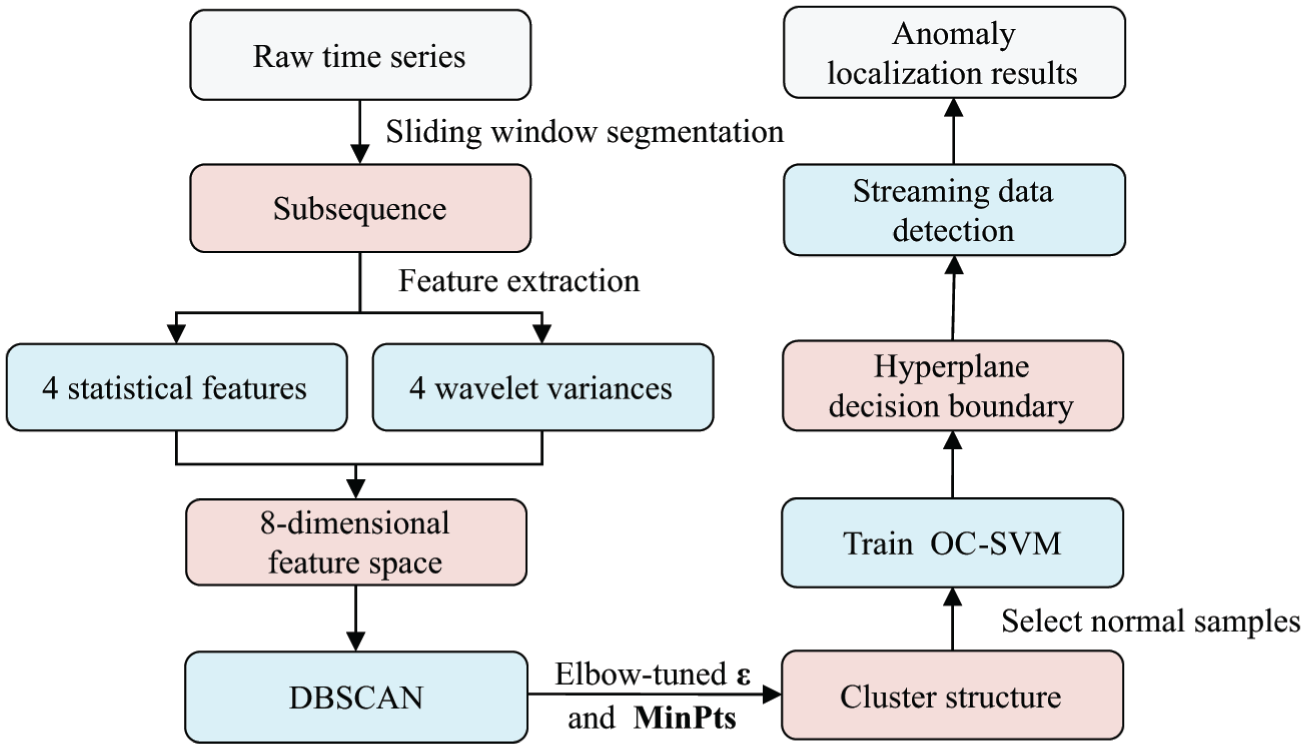
Anomaly detection framework.

Statistical parameter

Statistical parameters exhibit differentiated sensitivity to different types of time-series anomalies,¹ which play an important role in anomaly detection.

For missing-value anomalies, common indicators include the number of not-a-number values or constant values and the differential. A higher count of the former indicates more severe data loss, which affects data integrity. The differential measures the magnitude of change between adjacent points. When missing values or constant segments are present, the differential shows significant abnormal fluctuations, facilitating the detection of missing segments.

For outlier-type anomalies, differential and extremes are the most sensitive. Outliers exhibit substantial differences from neighboring data, resulting in abnormal differential values, while extremes directly reflect local peaks, effectively aiding in identifying points deviating from the normal distribution.

For drift-type anomalies, the most sensitive features include difference, extreme value, mean value, and cross-entropy. The difference measures deviations between data segments and the normal state; drift significantly alters the distributions of both the mean and the extreme values. Cross-entropy quantifies differences in probability distributions, enabling the detection of global distribution changes.

For trend anomalies, difference, extreme value, mean value, and quantile are more sensitive. The difference reflects the rate of trend change, the mean represents the overall level, extremes capture extreme points within the trend, and quantiles describe distributional changes from different positions in the data.

The sensitivities of different anomaly types to various statistical parameters are integrated in the study. Based on repeated experiments, four statistical features from subsequences are selected: (1) variance of differentials, (2) maximum value difference, (3) mean value, and (4) mean value divided by the 80th percentile.

Wavelet variance

The wavelet analysis process for time series is as follows: Given a signal ${x (t), - \infty < t < \infty}$ , Wavelet coefficients ${W (λ, t) : λ > 0, - \infty < t < \infty}$ can be obtained through the continuous wavelet transform. The calculation formula is as follows:

W (λ, t) = \int_{- \infty}^{\infty} ψ_{λ, t} (u) x (u) du

(1)

where $ψ_{λ, t} (u) \equiv \frac{1}{\sqrt{λ}} ψ (\frac{u - t}{λ})$ , $λ$ is the transformation scale of the wavelet coefficient, and $t$ is the position of action. The function $ψ (\cdot)$ satisfies $\int_{- \infty}^{\infty} ψ (u) du = 0$ and $\int_{- \infty}^{\infty} ψ^{2} (u) du = 0$ .

The maximum overlap discrete wavelet transform (MODWT) proposed by Percival and Walden²⁹ improves the boundary handling mechanism to generate the same number of wavelet coefficients as the number of observations in the original time series, while offering the following advantages: (1) Eliminating time-shift sensitivity and maintaining translation invariance. (2) Signal feature alignment is achieved using zero-phase filters. (3) Supporting the analysis of data with arbitrary length and suppressing boundary effects effectively. (4) Providing more refined multiscale decomposition capabilities.

Let ${{\hat{h}}_{l}, l = 0, 1, \dots, L}$ be the MODWT wavelet filter associated with scale $t_{j} = 2^{j - 1}$ , with length $L_{j}$ . Then, the wavelet coefficients of the random process $X_{t}$ at the $j$ th layer are:

W_{j, t} = \sum_{l = 0}^{L_{j}} {\hat{h}}_{j, l} X_{t - l^{j}}

(2)

The corresponding wavelet variance is defined as:

W_{j, t} = \sum_{l = 0}^{L_{j}} {\hat{h}}_{j, l} X_{t - l}

(3)

where $W_{j, t}^{2}$ is the wavelet coefficient at time $t$ , and $M_{j} = N - L_{j} + 1$ is the number of effective coefficients after removing the boundary coefficients. This variance satisfies $\sum_{j = 0}^{\infty} u_{X}^{2} (τ_{j}) = var {X_{t}}$ , meaning that the wavelet variance decomposes the cross-scale variance of a random process.

To avoid high-frequency noise interference, MODWT is employed for wavelet analysis, and wavelet variances are calculated on each frequency band. While preserving the multi-scale characteristics of the signal, the feature dimension after the wavelet transform is compressed to the scale of frequency bands. Based on the characteristics of the dataset, four wavelet variances from subsequences are finally adopted, which, together with the four statistical features, form an eight-dimensional feature space.

DBSCAN algorithm

DBSCAN is a density-based unsupervised clustering algorithm³⁰ that determines cluster structures based on local density and marks sparse region samples as outliers. Its core concepts include $ε$ -neighborhoods, core points, and density connectivity. If a sample point $p$ has at least $MinPts$ samples within a neighborhood of radius $ε$ , then $p$ is a core point; non-core points in the $ε$ -neighborhood are boundary points and are assigned to the nearest core point cluster, while the remaining points are outliers. The algorithm recursively expands clusters based on the density accessibility of core points, forming clusters connected by chained paths of core points, thereby effectively identifying clusters of arbitrary shapes and exhibiting strong noise resistance.

DBSCAN is suitable for handling non-convex clusters and noisy data. In addition, DBSCAN can complete the clustering process without pre-specifying the number of clusters. Regarding parameters, the parameters are optimized using the elbow method and feature dimension to determine the optimal parameter $(ε, MinPts)$ .

OC-SVM algorithm

Support Vector Machine (SVM) is a widely used supervised learning method that maps data into a high-dimensional space via kernel functions to construct a hyperplane for nonlinear classification. OC-SVM is an extension of SVM designed for scenarios where only single-class samples are available, primarily applied in unsupervised tasks such as anomaly and outlier detection. Unlike conventional SVM, OC-SVM has only one classification objective and can be trained exclusively on normal data. Its aim is to construct a high-dimensional hyperplane in the feature space that maximizes the distance from the origin while enclosing as many normal data points as possible, thereby excluding anomalies. For a new sample, determining whether it lies within the hyperplane enables anomaly detection.

The OC-SVM commonly uses a radial basis function (RBF) kernel to capture nonlinear decision boundaries in high-dimensional feature spaces. Its performance is governed by two parameters: $ν$ (range in 0–1), which balances sensitivity and robustness, and $γ$ , which defines the kernel width and the influence range of each sample.

Herein, a subset of normal samples with core density connectivity was first selected by DBSCAN and then employed for OC-SVM model training. The model learned the distributional characteristics of normal data in the feature space and optimized the boundary to generate the hyperplane decision function. After training, the model and its corresponding standardization parameters were saved for subsequent real-time anomaly detection. This approach not only ensures high anomaly detection accuracy but also establishes a reusable streaming detection framework, significantly improving efficiency and providing interpretable decision criteria for the subsequent repair stage.

Data repair method based on PatchTST

In recent years, transformer-based models have dominated the field of time-series research due to their outstanding performance.³¹ Among these, PatchTST³² significantly improves the performance and efficiency of transformer series models through an innovative patch embedding mechanism. The PatchTST architecture is extended to SHM and employed as a temporal feature extractor for data repair tasks in the study.

The PatchTST-based sensor mapping model effectively captures the spatiotemporal correlations between different sensors, providing precise references for the repair process. The theoretical foundation of this method lies in the significant correlation between spatial neighboring sensor monitoring data. Deep neural networks trained on massive lossless data can effectively reconstruct abnormal data segments. The specific model architecture and training process will be detailed in the following subsections.

PatchTST model framework

The success of the transformer architecture³³ in natural language processing (NLP) and CV has driven its application in time-series analysis, demonstrating strong sequence modeling capabilities and scalability. Research indicates that in time-series forecasting (TSF) tasks, its performance has surpassed methods such as the temporal convolutional network and recurrent neural network.^34,35

However, the decomposition linear model,³⁶ by introducing a simple multilayer perceptron architecture, achieves superior performance over contemporary transformer models in TSF tasks, raising questions about the effectiveness of transformers. To address this, PatchTST³² employs an innovative patch embedding mechanism combined with a channel-independent strategy, achieving improvements in both performance and efficiency for TSF tasks. Compared to channel-mixing methods, channel-independent modeling reduces cross-channel interference, while patch embedding preserves semantic information by dividing local segments, significantly shortening input length and improving computational efficiency.

The overall architecture of PatchTST includes a normalization layer, an embedding layer, a transformer encoder, and an output layer. Figure 2 illustrates the forward propagation process of this architecture on a mini-batch of data.

Figure 2.

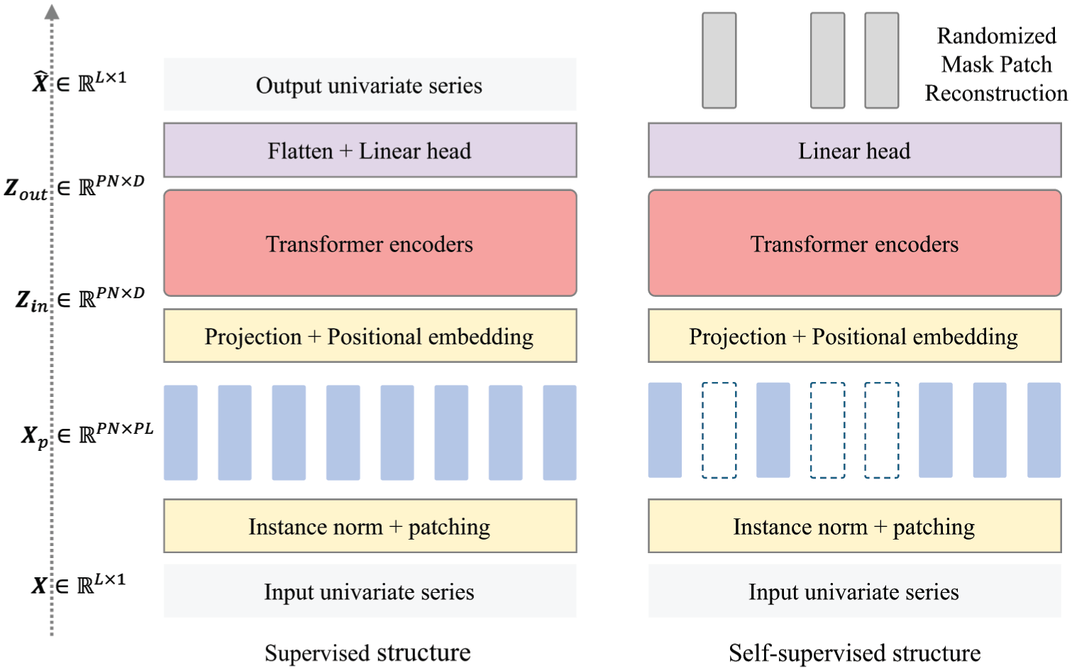
PatchTST model framework.

PatchTST model training

In general, a large-scale and pre-trained model shows scalability and generalization in few-shot learning. However, in the field of time-series analysis, their effectiveness is often constrained by the limited availability of downstream task data. To address this limitation, self-supervised learning has emerged as a key approach, enabling the extraction of high-level representations from unlabeled data and substantially enhancing model generalization in data-scarce scenarios. As a representative method, masked autoencoders randomly mask portions of the input and reconstruct the missing segments. This approach has achieved notable success in both NLP and CV,^37,38 and has also shown significant performance gains in time-series classification and regression tasks.³⁹

Considering the characteristics of time series, PatchTST employs non-overlapping patch segmentation combined with partial patch random masking and performs self-supervised representation learning using mean squared error (MSE) loss. This method overcomes the limitations of traditional time-series representation learning methods through two innovative designs: (1) Replacing point-level masking with patch-level masking to enhance local semantic extraction capabilities; (2) Introducing a D × PL linear layer to effectively reduce overfitting risks (as shown in Figure 2).

Based on this, PatchTST adopts a two-stage training strategy. First, in the self-supervised pre-training stage, the model learns general representation features of time series through a random masking patch reconstruction mechanism, maintaining good generalization ability under conditions of scarce labeled data. Subsequently, in the supervised fine-tuning stage, the weights of the linear layer are optimized for specific tasks, achieving rapid adaptation and further improving prediction accuracy and stability.

Data cleaning process

Existing data cleaning methods face several challenges: complex anomaly detection models with limited interpretability, strong spatial dependency of anomaly repair, insufficient exploitation of spatiotemporal features, and the lack of efficient synchronous repair. To address these issues, signal processing techniques are integrated with DL algorithms, and a full-process data cleaning framework is proposed in the study.

As shown in Figure 3, this framework employs an intelligent distortion discrimination method and a deep temporal model trained with multi-sensor spatiotemporal correlations. It establishes a detect-then-repair subsequence-level data cleaning strategy that balances algorithmic accuracy and computational efficiency, providing an effective and accurate solution for the quality analysis of large-scale monitoring data. The technical workflow is as follows:

Anomaly detection stage: An intelligent method for detecting data distortion is proposed, which involves clustering sub-sequences based on statistical features and wavelet variances, and obtaining a hyperplane decision boundary using OC-SVM. By integrating time-domain and frequency-domain features, efficient anomaly detection is achieved to precisely locate the data segments requiring repair.

Data repair stage: Anomalous data is removed from the training dataset. Data reconstruction is performed using pre-trained time-series models and multi-sensor mapping relationships, combined with spatiotemporal features to repair distorted data segments. To enhance the reliability of the repair results, the hyperplane decision boundary constructed by OC-SVM is further introduced. By performing the same feature extraction on the repaired segments, the hyperplane is used to score and distinguish the candidate repair results. The result closest to the normal data distribution is prioritized as the final output, ensuring that the repair process is more robust and interpretable.

Figure 3.

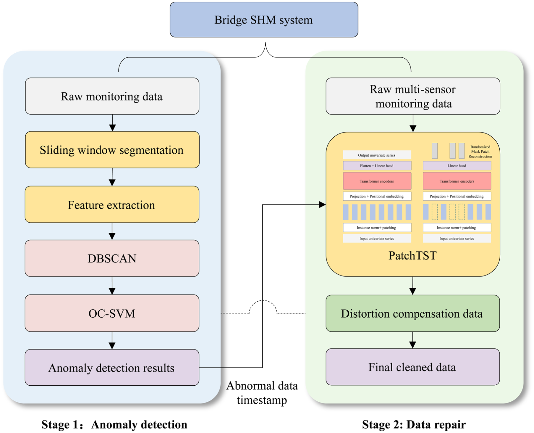
Data cleaning methodology framework.

Case study

Background of field test

In this study, the JJB is selected as the research object. The bridge serves as the main bridge of the right branch self-anchored bridge of the Nanjing Yangtze River tunnel project. It is a single-pylon self-anchored suspension bridge, and the first three orders natural frequencies are 0.435, 0.684, and 1.286 Hz, respectively. The bridge spans are arranged as (35 + 77 + 60 + 248 + 35) m as shown in Figure 4. The bridge consists of two steel box main girders connected by multiple transverse beams, with a clear spacing of 8.2 m. The sensor configuration of the JJB is symmetrically arranged on the upstream and downstream sides.

Figure 4.

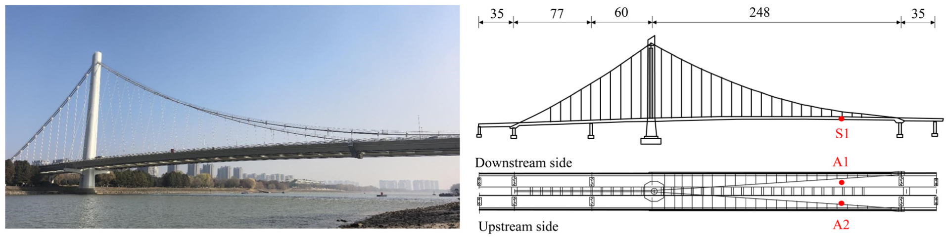
Schematic diagram of the Jiajiang Bridge.

To validate the effectiveness of the proposed data cleaning framework, a case study was conducted using acceleration data obtained from the health monitoring system of the JJB in October 2023. The data were collected from the S1 section at the 3/4 position of the JJB main span, with an original sampling frequency of 20 Hz. The normalized root mean square error (NRMSE) is adopted to evaluate the accuracy of the results, as it is commonly used in the error assessment of bridge acceleration data⁴⁰:

NRMSE = \frac{\sqrt{\frac{1}{n} \sum_{i = 1}^{n} {(y_{i} - {\hat{y}}_{i})}^{2}}}{\max (y) - \min (y)}

(4)

where $y_{i}$ and ${\hat{y}}_{i}$ denote the reference and repaired (predicted) values of the $i$ -th sample, respectively. $n$ is the total number of samples.

Results of field validation

Anomaly detection results

In this section, an OC-SVM hyperplane is trained on the October 1–7 dataset from sensor A1 at the S1 section of the JJB. The trained model is then applied to detect anomalies in the A1 data recorded on October 31. In addition, drift is artificially introduced in the dataset of October 1–7 to simulate the learning challenges posed by abnormal raw data (Figure 5(a)). After applying DBSCAN to the subsequences of the October 1–7 data to obtain a normal dataset, an OC-SVM is trained on the normal data to construct a hyperplane for anomaly detection. 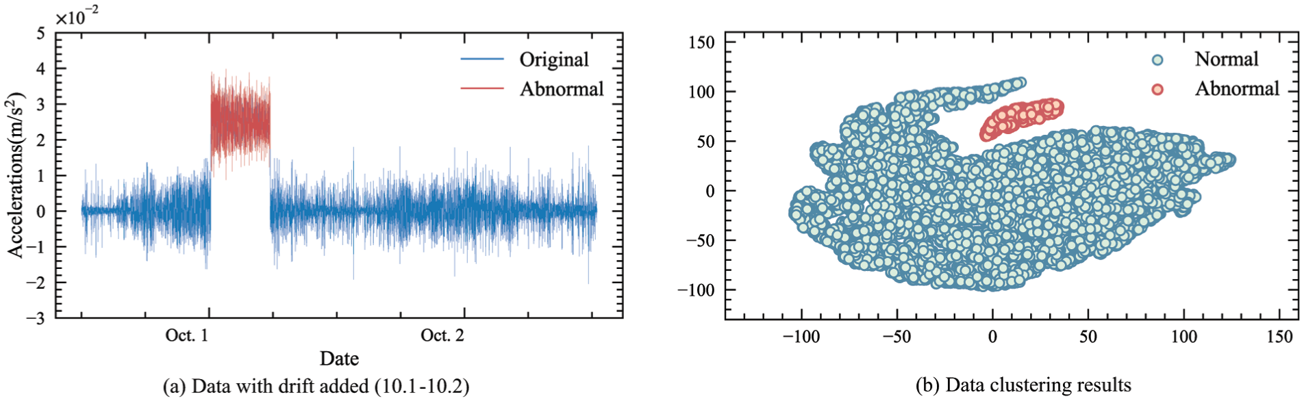The subsequence window length is set to 256, and the parameters $(ϵ, MinPts)$ are determined as $(3, 10)$ using a joint grid search, with the optimal silhouette coefficient reaching 0.7259. The OC-SVM model employs an RBF kernel, with key parameters set as $ν = 0.01$ , and $γ$ automatically determined from the data variance. The RBF kernel was selected because the 8-dimensional features derived from wavelet variance and statistical measures usually show a nonlinear distribution in real monitoring data. Compared with a linear kernel, it is more suitable for learning a flexible boundary around normal samples while maintaining a good balance between detection accuracy and computational cost.

Figure 5.

Acceleration data from sensors A1. (a) Data with drift added (10.1–10.2) and (b) Data clustering results.

Since the hyperplane resides in an eight-dimensional space, direct visualization is not feasible. Therefore, t-distributed stochastic neighbor embedding is applied to the clustering results of the October 1–7 data for dimensionality reduction, as shown in Figure 5(b). In this figure, the hyperplane encloses the normal clusters, effectively distinguishing normal data from anomalies.

Since the restored data usually lacks reference values, anomalies were artificially added to facilitate subsequent verification. Furthermore, to examine the robustness of the subsequence-based anomaly detection method in handling distorted data, five types of abnormal conditions were artificially generated into the October 31 dataset: strong interference, drift, missing, trend anomaly, and outliers. The time series was partitioned into subsequences of 102,400 points (approximately 80 min), which were used as the basic units for both anomaly injection and detection. These anomalies were implemented as follows: (1) Strong interference was simulated by adding Gaussian white noise to a randomly selected contiguous interval. (2) Drift anomalies were introduced by adding a constant offset to a contiguous segment. (3) Missing anomalies were created by replacing contiguous intervals with zeros; (4) Trend anomalies were produced by superimposing a linearly varying term on a contiguous segment; (5) Outliers were generated by abruptly perturbing a small number of randomly selected discrete samples within a subsequence.

Figure 6 presents the detection results of abnormal segments under the five operating conditions. From the detection results, it is evident that the proposed subsequence-based anomaly detection method can accurately detect distortion data generated under five abnormal conditions. By leveraging the OC-SVM hyperplane decision boundary, the method achieves high-precision streaming detection while balancing recognition efficiency and interpretability. It demonstrates stable detection performance and strong generalization capability across the overall task, providing a reliable reference for subsequent data repair.

Figure 6.

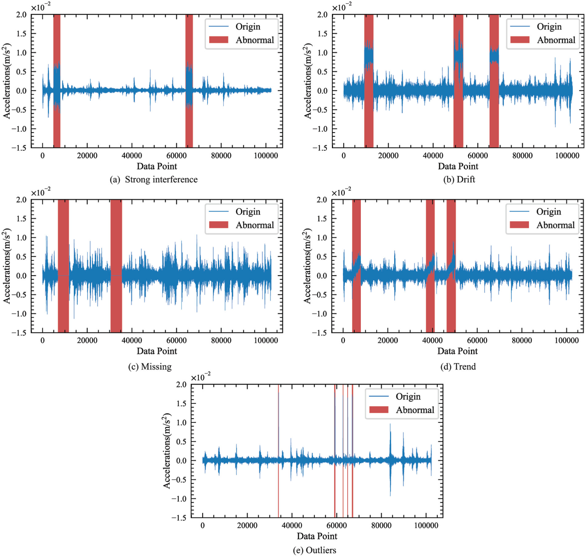
Results of detection for each type of distortion. (a) Strong interference, (b) Drift, (c) Missing, (d) Trend, and (e) Outliers.

It should be noted that the proposed method is highly extensible. Although an 8-dimensional feature vector is adopted in this study, this choice reflects a balance between detection capability, interpretability, and computational efficiency for the specific dataset and distortion types considered here. In more complex monitoring scenarios, additional time–frequency statistical features can be incorporated to enrich subsequence representation and improve sensitivity to common distortion patterns.

Similarly, the sliding-window configuration can be flexibly adjusted according to sampling characteristics, anomaly duration, and deployment requirements. In this study, a window length of 256 with a stride of 256 was selected because it achieves a suitable balance between detection performance and computational cost for the current dataset and model setting. More generally, different window lengths capture information at different temporal scales, while the stride affects coverage density and computational burden. Therefore, in practical applications, it is recommended to combine multiple subsequence window sizes with appropriate stride settings for multiscale feature analysis, thereby improving the robustness and overall detection performance of the method.

Data repair results

To ensure the reliability of the multi-sensor mapping model, sensor groups with highly correlated monitoring data are preferentially selected for sample screening and model training. Considering the spatial symmetry of sensor deployment, acceleration data from sensors A1 and A2 at the S1 section of the JJB collected on October 1–7 were used for analysis. After distorted subsequences are located and removed using subsequence-based anomaly detection, 28,000 normal samples are randomly selected for model training. The deep mapping model constructed from distortion-free data can subsequently be used for distortion repair. Figure 7 shows the frequency distribution histograms of sensors A1 and A2, illustrating the data distribution characteristics and the statistical similarity between the two sensors.

Figure 7.

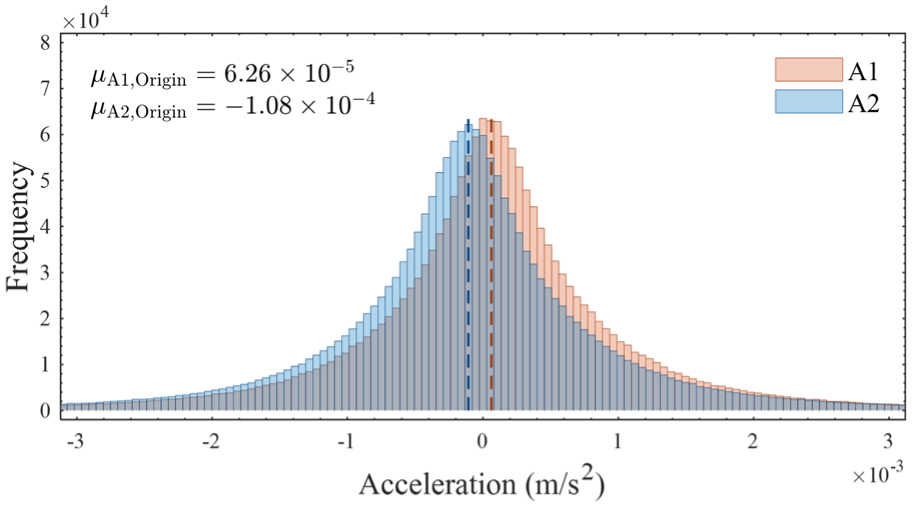
Frequency distribution histograms of sensors A1 and A2.

The PatchTST model was implemented in Python using the PyTorch framework. The optimization objective was the MSE, and the adaptive moment estimation optimizer was adopted. The learning rates for the two training stages, pretraining and fine-tuning, were set to 0.005 and 0.0005, respectively, with 300 epochs in each stage. In the task setting, the model takes 256 time steps from sensor A2 as input to predict the corresponding 256 time steps of sensor A1, ensuring consistency between the subsequence partition length and the clustering window size. During training, the batch size was 128, and the dataset was divided into training and validation sets in a 4:1 ratio. The experiments were carried out on a workstation configured with an Intel Core i7-12,700KF CPU (12 cores, 20 threads) and an NVIDIA RTX 4060 Ti GPU (8 GB).

In addition, instance normalization was applied for data standardization before feeding the sequence samples into the network. Figure 8 shows the loss reduction curves of the PatchTST model during both self-supervised pretraining and supervised training, indicating that the neural network parameters were effectively optimized.

Figure 8.

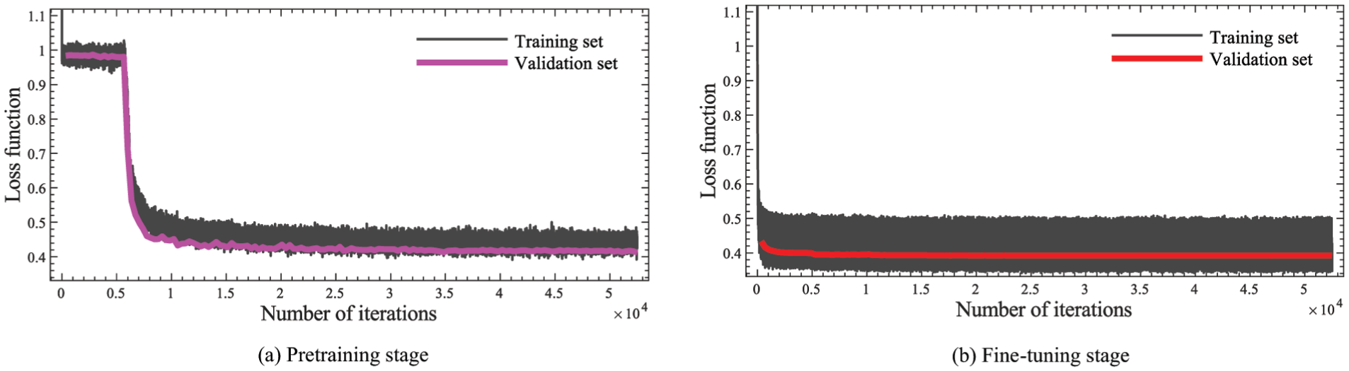
Loss function descent curve. (a) Pretraining stage and (b) Fine-tuning stage.

In this section, acceleration monitoring data from sensor A1 on October 31 are used to evaluate the data repair performance of the deep mapping model constructed with PatchTST. To verify the model’s generalization capability, the entire day’s data are adopted, and the trained PatchTST model is employed to reconstruct the A1 sensor data based on the input from the A2 sensor. To further improve repair accuracy, PatchTST performs 100 predictions on the same input. The results are then evaluated using the trained OC-SVM hyperplane, with the scores determined by the distance from the hyperplane. The prediction with the highest score is selected as the final repair output, which is considered closest to the normal data distribution. Subsequently, regression modeling is conducted based on the repaired results and the original normal data, and the model’s predictive performance is validated through their comparison. In addition, the results of direct prediction are compared with those of repair evaluated by the OC-SVM hyperplane.

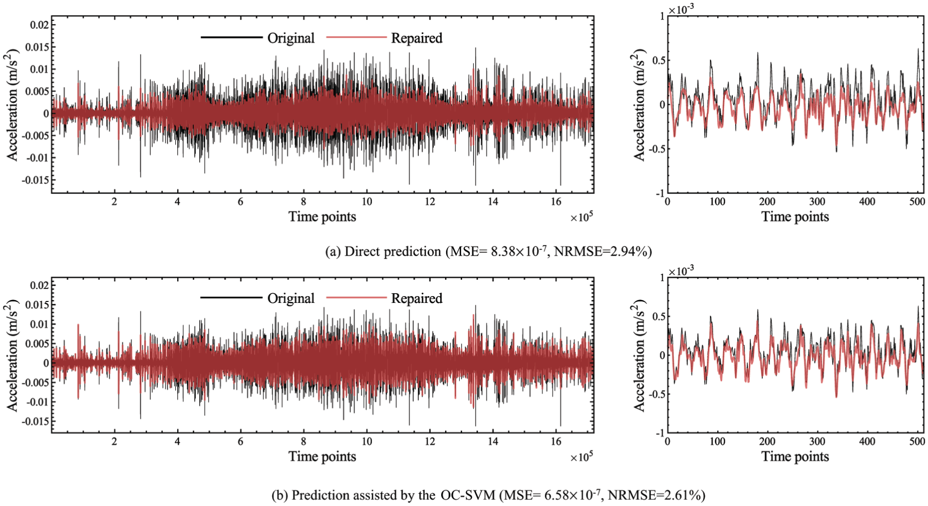
As shown in Figure 9, the model achieves an MSE of $8.38 \times 10^{- 7}$ and an NRMSE of 2.95% under direct prediction. After incorporating the OC-SVM hyperplane and selecting the optimal result, the MSE decreases to $6.58 \times 10^{- 7}$ and the NRMSE to 2.61%, decreasing by approximately 21.5% and 11.5%, respectively. These results demonstrate that the model exhibits strong global regression performance, with the predicted data being highly consistent with the actual data in overall distribution.

Figure 9.

Data regression results display.

The repaired time-series segments were extracted and output according to the anomaly timestamps identified during detection. The repaired data were then compared with the ground truth to evaluate the model’s restoration performance.

Figure 10 shows the repair results of the anomalous segments corresponding to the five conditions localized above. From the restoration results, it can be observed that under various abnormal conditions, the repaired data exhibit high temporal-domain consistency with the ground truth. Moreover, as the length of the missing segments increases, the restoration performance remains stable without significant degradation. This indicates that the proposed deep mapping model can effectively handle large-scale distorted data restoration tasks, demonstrating strong robustness. Further quantitative analysis using metrics such as NRMSE confirms the method’s strong performance across different distortion types. The repaired data are highly consistent with the original normal data in both the time and frequency domains. This consistency verifies the method’s applicability to real-world bridge monitoring data and establishes a complete framework for anomaly detection and data restoration.

Figure 10.

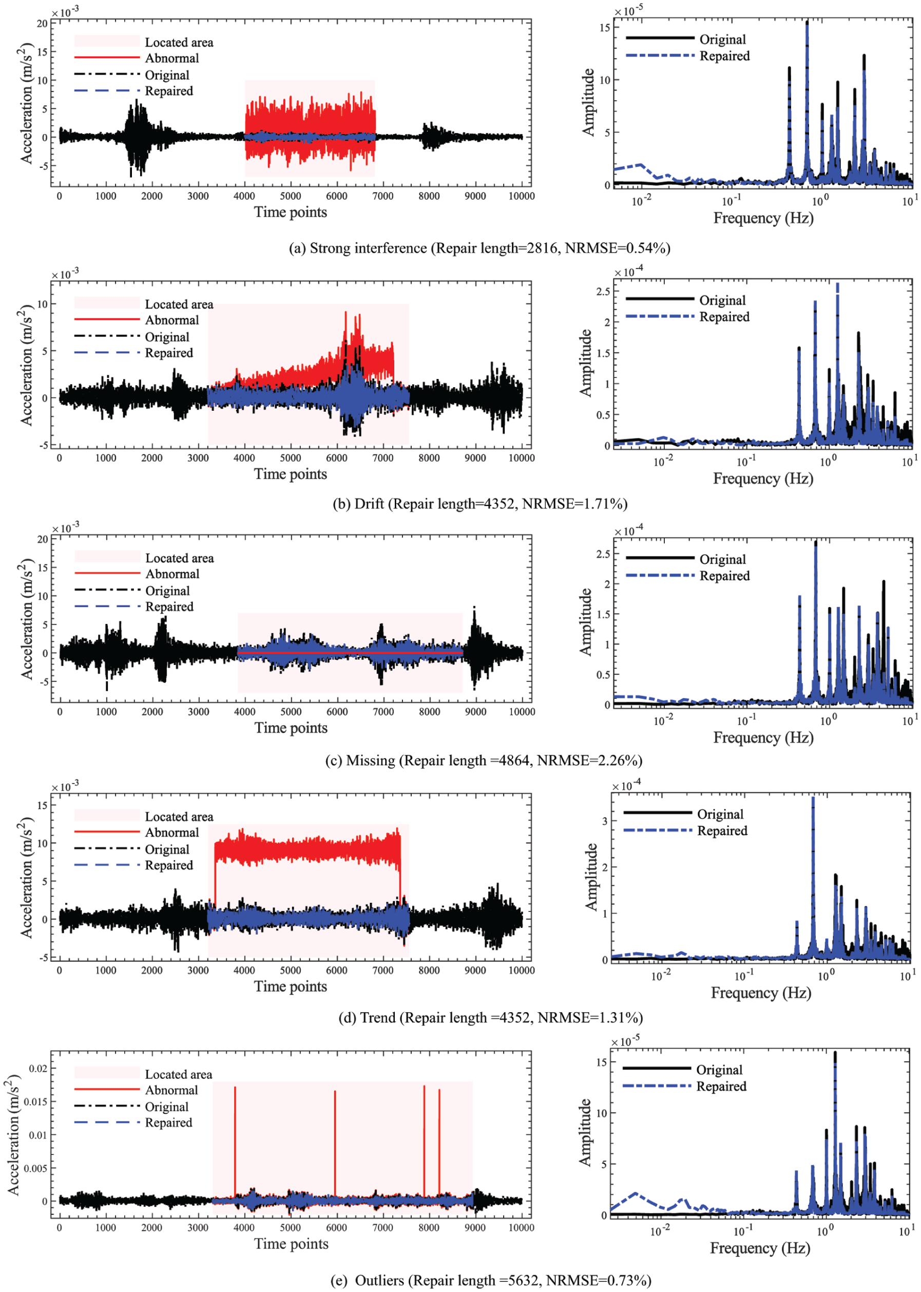
Cleaning performance for each abnormal condition. (a) Strong interference (repair length = 2816, NRMSE = 0.54%), (b) Drift (repair length = 4352, NRMSE = 1.71%), (c) Missing (repair length = 4864, NRMSE = 2.26%), (d) Trend (repair length = 4352, NRMSE = 1.31%), and (e) Outliers (repair length = 5632, NRMSE = 0.73%).

Conclusion

A complete framework for subsequence-level data cleaning that follows a “detect-repair” strategy is proposed in the study, aiming to improve data quality through efficient anomaly detection and precise repair. The validation on field monitoring data demonstrates the robustness and effectiveness of the proposed method for automated cleaning of large-scale data. The main conclusions of this method are as follows:

Subsequence feature vectors are constructed based on wavelet variances and statistical parameters, and an efficient anomaly detection method is developed by integrating DBSCAN and OC-SVM. It can accurately locate various types of anomalies and eliminate abnormal samples during the training stage, thereby ensuring the reliability of the input data.

The hyperplane decision boundary constructed based on OC-SVM enables fast streaming detection of subsequent data, meeting real-time monitoring requirements. It can evaluate repair results by identifying the reconstructed outputs that best match the normal data distribution, thus enhancing repair accuracy and reliability.

Combining the channel-independent modeling characteristics of PatchTST with the spatial symmetry of the sensors on the JJB, a one-to-one nonlinear mapping model is constructed to effectively avoid cross-channel noise interference. The proposed method demonstrates consistent performance across different repair lengths.

Five types of abnormal conditions were artificially generated, and the corresponding distorted segments were subsequently repaired. Using data from sensor A1 on October 31 as an example, the method accurately located and repaired multiple types of anomaly data. The model achieved an NRMSE of 2.61%, demonstrating excellent cleaning performance in practical bridge monitoring scenarios.

Footnotes

ORCID iD

Dongming Feng

Funding

The authors disclosed receipt of the following financial support for the research, authorship, and/or publication of this article: This article was supported by the National Key Research and Development Program of China (2023YFC 3805900), the Transportation Science and Technology Project of Jiangsu Province (2024Y15), and the Science and Technology Research and Development Program of China Railway Co., Ltd (P2022G054).

Declaration of conflicting interests

The authors declared no potential conflicts of interest with respect to the research, authorship, and/or publication of this article.

References

Yang

Ding

Jiang

, et al. A two-stage data cleansing method for bridge global positioning system monitoring data based on bi-direction long and short term memory anomaly identification and conditional generative adversarial networks data repair. Struct Control Health Monit 2022; 29(9): e2993.

Katicha

Flintsch

Bryce

, et al. Wavelet denoising of TSD deflection slope measurements for improved pavement structural evaluation. Comput Aided Civ Infrastruct Eng 2014; 29(6): 399–415.

Petersen

ØW

Øiseth

Nord

, et al. Estimation of the full-field dynamic response of a floating bridge using Kalman-type filtering algorithms. Mech Syst Signal Process 2018; 107: 12–28.

Choi

Shon

Byon

, et al. Enhanced application of principal component analysis in machine learning for imputation of missing traffic data. Appl Sci 2019; 9(10): 2149.

Brauckhoff

Salamatian

May

. Applying PCA for traffic anomaly detection: problems and solutions. In IEEE INFOCOM 2009, 2009, pp. 2866–2870. IEEE.

Gilda

Slepian

. Automatic Kalman-filter-based wavelet shrinkage denoising of 1D stellar spectra. Mon Not Royal Astron Soc 2019; 490(4): 5249–5269.

Wang

Zeng

Feng

, et al. Track vertical irregularity estimation for railway bridges using a novel and lightweight deep-learning architecture. Veh Sys Dyn 2024; 63(8): 1597–1624.

Wang

Zeng

Feng

. Deep learning-based damage assessment of hinge joints for multi-girder bridges utilizing vehicle-induced bridge responses. Eng Struct 2025; 333: 120148.

Zhang

Yuen

. Review of artificial intelligence-based bridge damage detection. Adv Mech Eng 2022; 14(9): 16878132221122770.

10.

Jia

. Deep learning for structural health monitoring: data, algorithms, applications, challenges, and trends. Sensors 2023; 23(21): 8824.

11.

Gul

Catbas

. Statistical pattern recognition for structural health monitoring using time series modeling: theory and experimental verifications. Mech Syst Signal Process 2009; 23(7): 2192–2204.

12.

Cui

Zeng

, et al. Damage detection of a cable-stayed bridge specimen based on unsupervised subdomain adaptation transfer learning. Eng Struct 2026; 346: 121660.

13.

Xiao

Cui

, et al. An unsupervised cross-domain method for bridge damage detection based on multichannel symmetric dot pattern feature alignment. Comput Aid Civ Infrastruct Eng 2025; 40(29): 5698–5718.

14.

Zhang

Noori

. Deep learning for data anomaly detection and data compression of a long-span suspension bridge. Comput Aid Civ Infrastruct Eng 2020; 35(7): 685–700.

15.

Bao

Tang

, et al. Computer vision and deep learning–based data anomaly detection method for structural health monitoring. Struct Health Monit 2019; 18(2): 401–421.

16.

Pan

Bao

. Transfer learning-based data anomaly detection for structural health monitoring. Struct Health Monit 2023; 22(5): 3077–3091.

17.

Tang

Chen

Bao

, et al. Convolutional neural network-based data anomaly detection method using multiple information for structural health monitoring. Struct Control Health Monit 2019; 26(1): e2296.

18.

Zhou

Jian

Xia

, et al. Transferring self-supervised pretrained models for SHM data anomaly detection with scarce labeled data. Struct Control Health Monit 2025; 2025(1): 2414195.

19.

Mao

Wang

Spencer

Jr . Toward data anomaly detection for automated structural health monitoring: exploiting generative adversarial nets and autoencoders. Struct Health Monit 2021; 20(4): 1609–1626.

20.

Arul

Kareem

. Data anomaly detection for structural health monitoring of bridges using shapelet transform. arXiv preprint arXiv:200900470 2020.

21.

Lai

Zha

, et al. Revisiting time series outlier detection: definitions and benchmarks. In: Thirty-fifth conference on neural information processing systems datasets and benchmarks track (round 1), 4 August 2021.

22.

Mejri

Lopez-Fuentes

Roy

, et al. Unsupervised anomaly detection in time-series: an extensive evaluation and analysis of state-of-the-art methods. Expert Syst Appl 2024; 256: 124922.

23.

Keogh

. Current time series anomaly detection benchmarks are flawed and are creating the illusion of progress. IEEE Trans Knowl Data Eng 2021; 35(3): 2421–2429.

24.

Ren

Chen

Sun

, et al. Incremental Bayesian matrix/tensor learning for structural monitoring data imputation and response forecasting. Mech Syst Signal Process 2021; 158: 107734.

25.

Deng

Zhai

, et al. Recovery of abnormal data for bridge structural health monitoring based on deep learning and temporal correlation. Sens Mater 2022; 34(12): 4491.

26.

Chen

Bao

, et al. LQD-RKHS-based distribution-to-distribution regression methodology for restoring the probability distributions of missing SHM data. Mech Syst Signal Process 2019; 121: 655–674.

27.

Wang

Z-W

X-F

Zhang

W-M

, et al. Deep learning-based reconstruction of missing long-term girder-end displacement data for suspension bridge health monitoring. Computers & Structures 2023; 284: 107070.

28.

Jeong

Ferguson

Hou

, et al. Sensor data reconstruction using bidirectional recurrent neural network with application to bridge monitoring. Adv Eng Inform 2019; 42: 100991.

29.

Percival

Walden

. Wavelet methods for time series analysis. Vol. 4. Cambridge University Press, 2000.

30.

Ester

Kriegel

Sander

, et al. A density-based algorithm for discovering clusters in large spatial databases with noise. In: KDD’96: proceedings of the second international conference on knowledge discovery and data mining, 2–4 August 1996, Vol. 96, pp. 226–231.

31.

Luo

Wang

. Moderntcn: a modern pure convolution structure for general time series analysis. In: The twelfth international conference on learning representations, 7–11 May 2024, pp. 1–43.

32.

Nie

Nguyen

Sinthong

, et al. A time series is worth 64 words: long-term forecasting with transformers. arXiv preprint arXiv:221114730 2022.

33.

Vaswani

Shazeer

Parmar

, et al. Attention is all you need. Adv Neural Inform Process Syst 2017; 30: 5998–6008.

34.

Zhou

Zhang

Peng

, et al. Informer: beyond efficient transformer for long sequence time-series forecasting. In: Proceedings of the AAAI conference on artificial intelligence, 2–9 February 2021, Vol. 35. pp. 11106–11115.

35.

Zhou

Wen

, et al. Fedformer: frequency enhanced decomposed transformer for long-term series forecasting. In: International conference on machine learning, 6–11 July 2026, pp. 27268–27286. PMLR.

36.

Zeng

Chen

Zhang

, et al. Are transformers effective for time series forecasting? In: Proceedings of the AAAI conference on artificial intelligence, 7–14 February 2023, Vol. 37, pp. 11121–11128.

37.

Chen

Xie

, et al. Masked autoencoders are scalable vision learners. In: Proceedings of the IEEE/CVF conference on computer vision and pattern recognition, 16–22 June 2024, pp. 16000–16009.

38.

Devlin

Chang

Lee

, et al. Bert: pre-training of deep bidirectional transformers for language understanding. In: Proceedings of the 2019 conference of the North American chapter of the association for computational linguistics: human language technologies, volume 1 (long and short papers), 2–7 June 2019, pp. 4171–4186.

39.

Zerveas

Jayaraman

Patel

, et al. A transformer-based framework for multivariate time series representation learning. In: Proceedings of the 27th ACM SIGKDD conference on knowledge discovery & data mining, 14–18 August 2021, pp. 2114–2124.

40.

Feng

. A comparative study of vehicle-bridge interaction dynamics with 2D and 3D vehicle models. Eng Struct 2023; 292: 116493.